Decision Tree Algorithms for Developing Rulesets for Object-Based Land Cover Classification

 ,
,  , ,
, ,  and
and 
Abstract
:
1. Introduction
2. Material and Methods
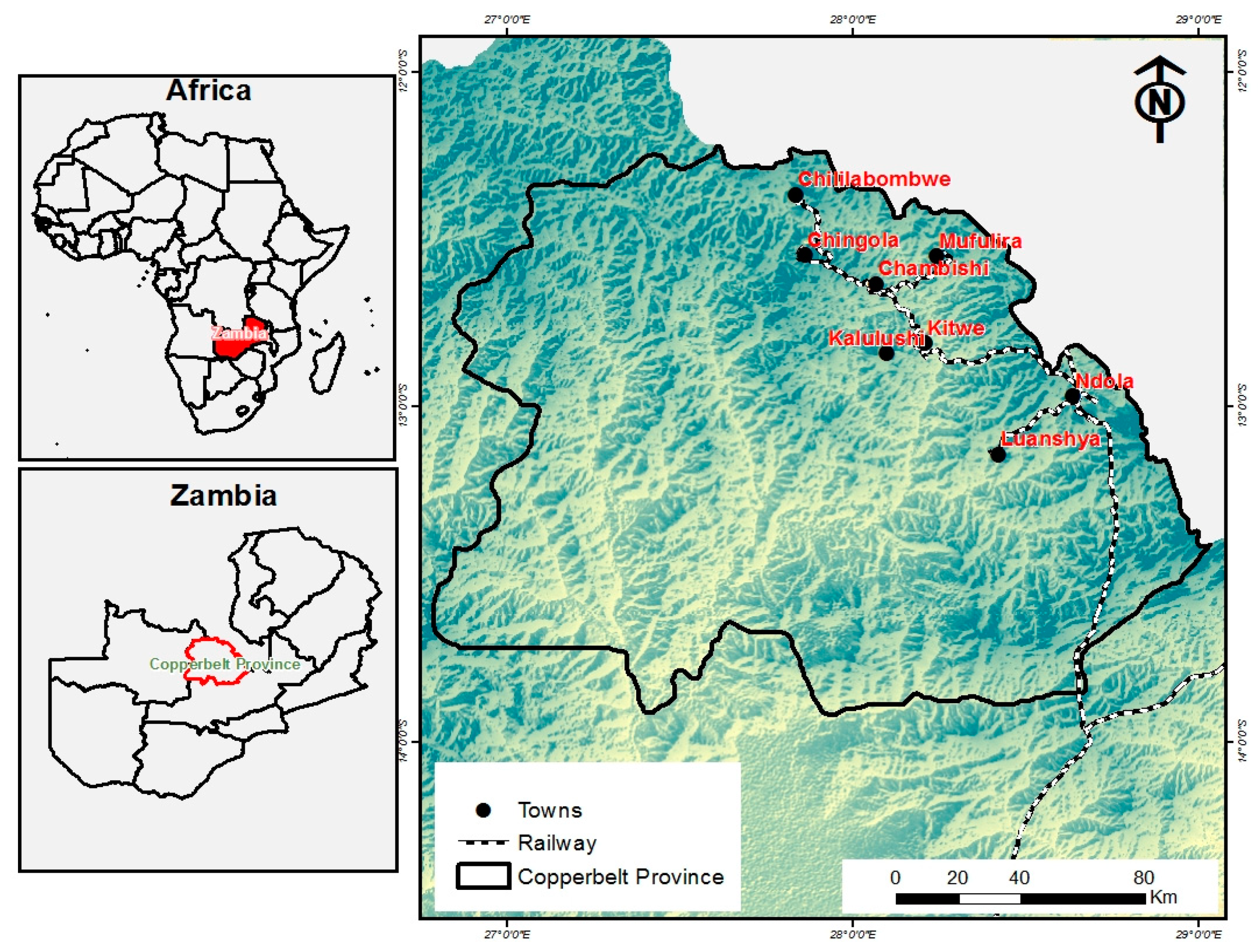
2.1. Study Site
2.2. Datasets
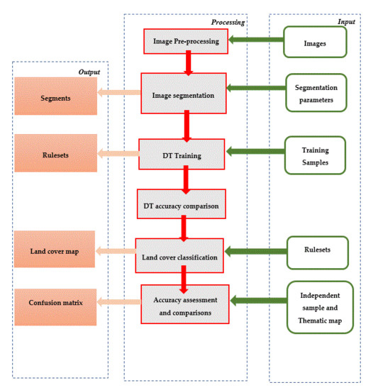
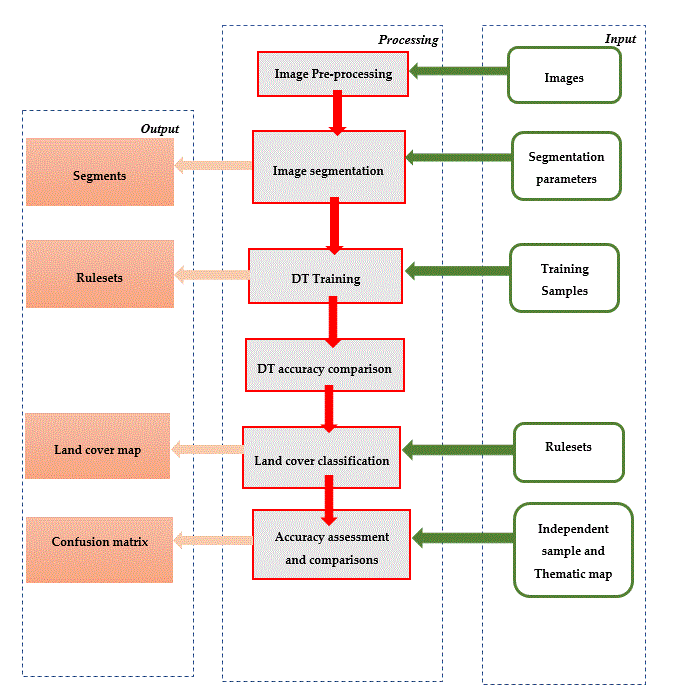
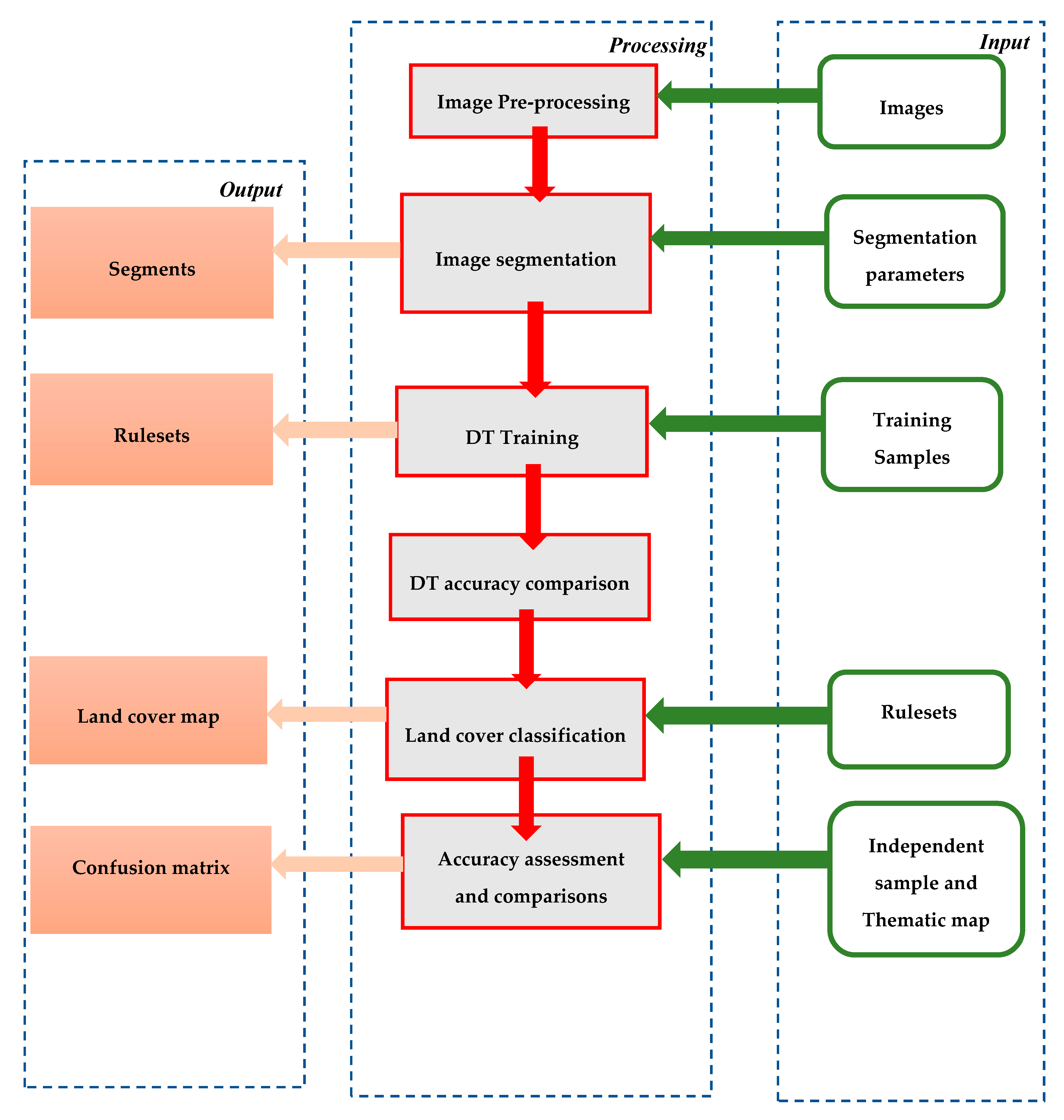
2.3. Methods
2.3.1. Pre-processing
2.3.2. Image Segmentation
2.3.3. Sample Selection and Feature Extraction
2.3.4. Decision Tree Algorithms
2.3.5. Assessing DT Accuracy
2.3.6. Assessing Thematic Map Accuracy
3. Results
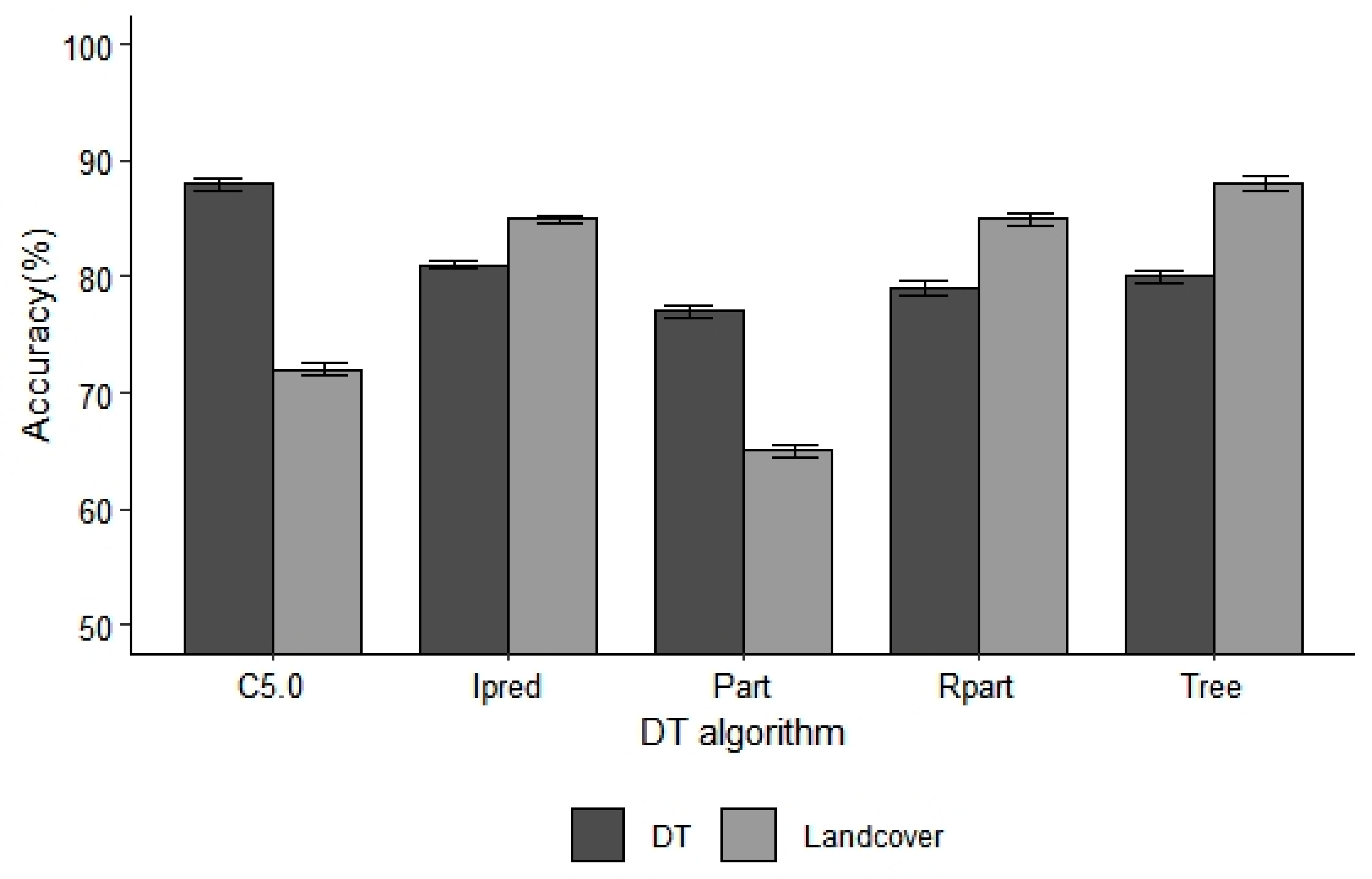
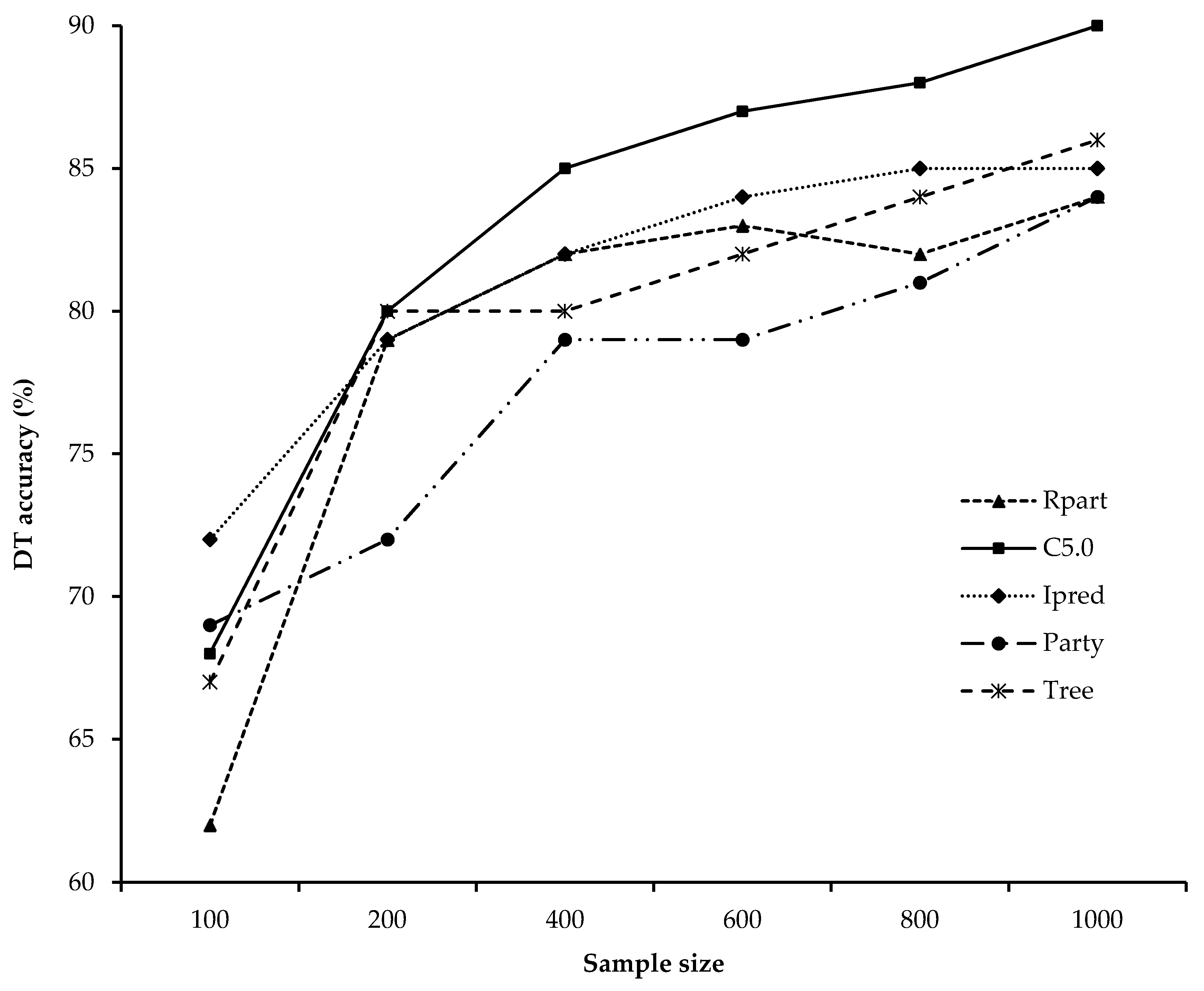
3.1. DT Accuracy
3.2. Thematic Map Accuracy
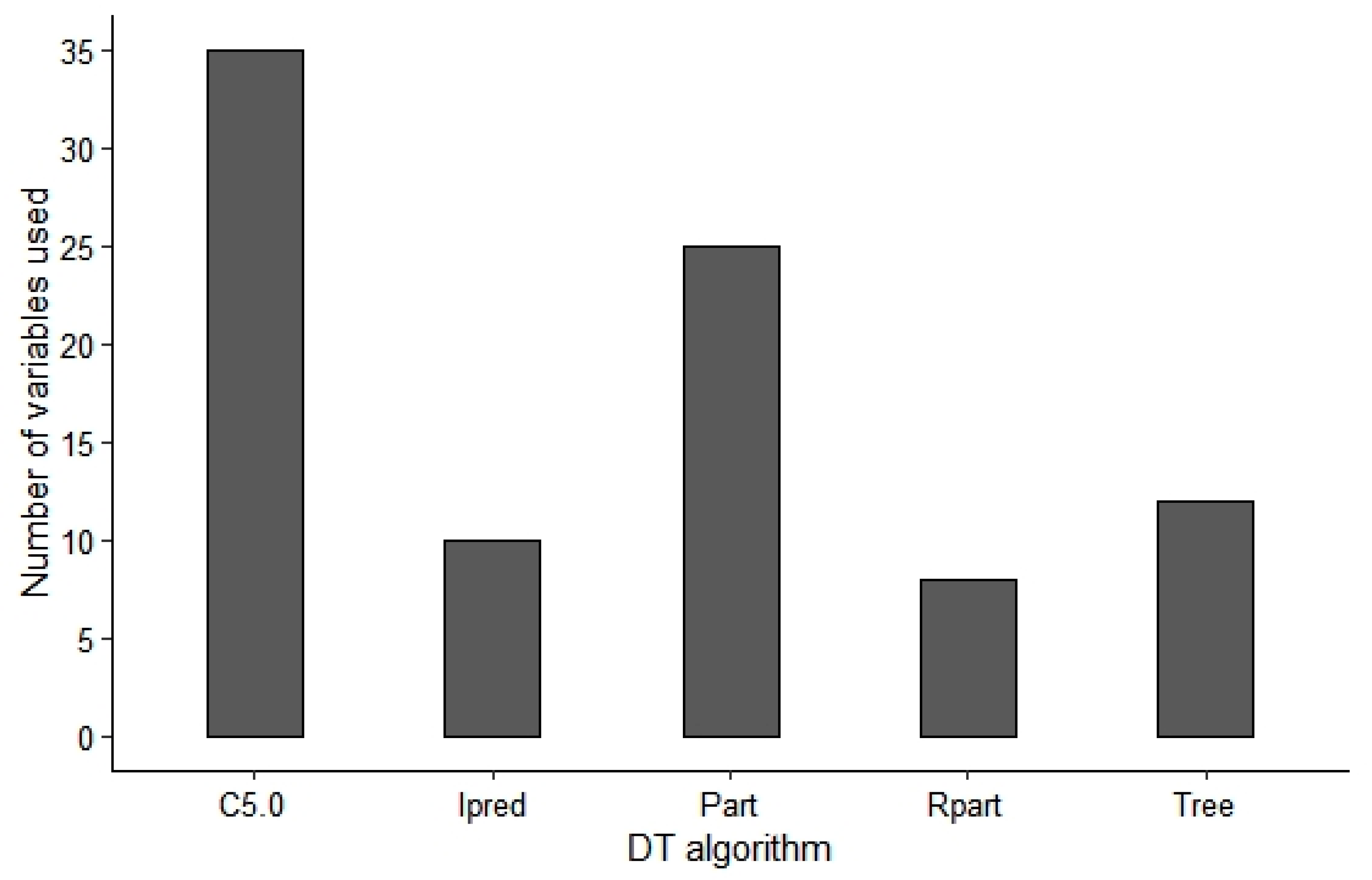
3.2.1. Number of Variables and Classification Accuracy
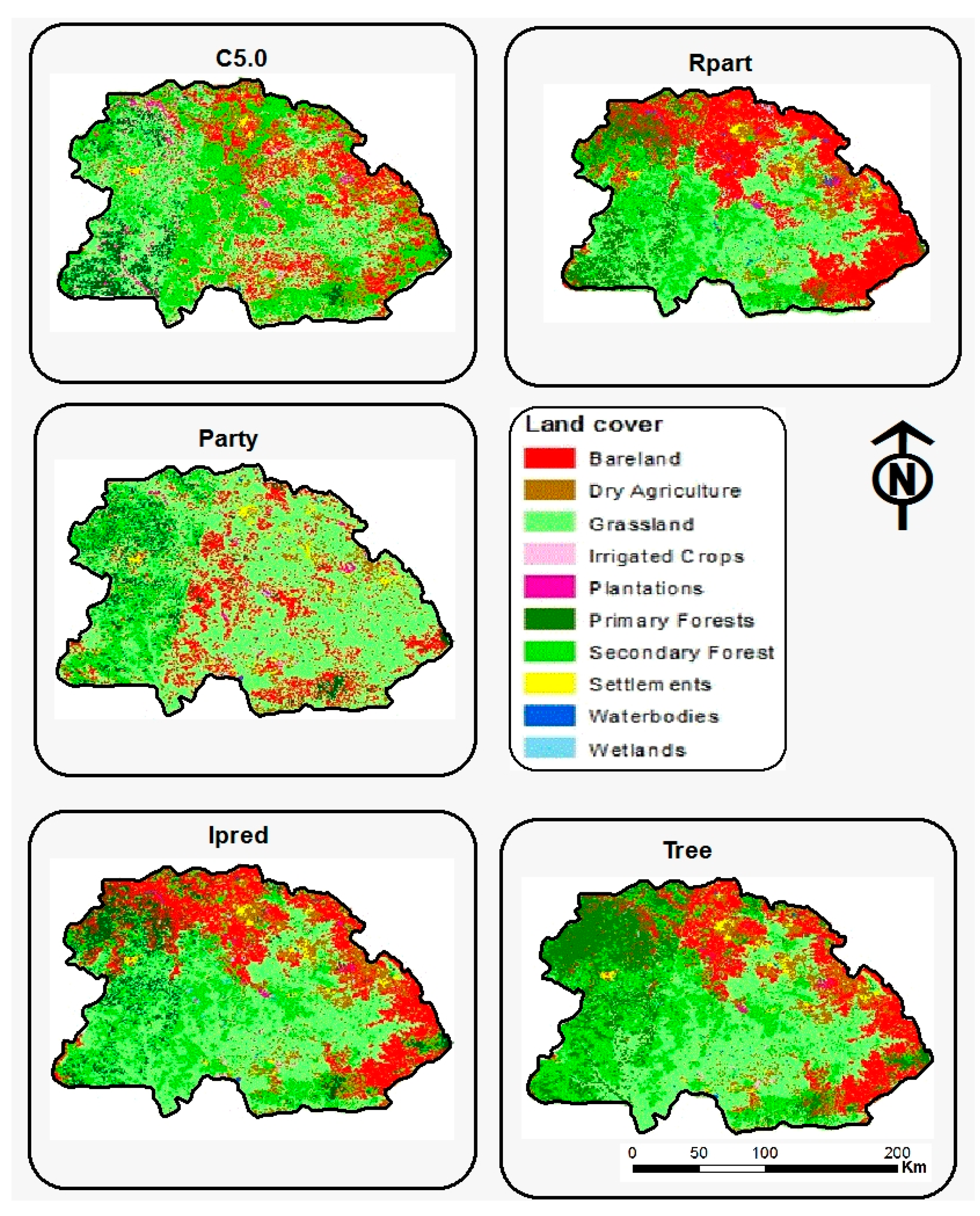
3.2.2. Thematic Map Classification Accuracy
3.2.3. Other DT Characteristics
4. Discussion
4.1. DT Accuracy
4.2. Thematic Map Classification Accuracy
4.3. Selecting the Best DT for Ruleset Development
5. Conclusions
Supplementary Materials
Author Contributions
Funding
Acknowledgments
Conflicts of Interest
References
- Kumar, R.; Nandy, S.; Agarwal, R.; Kushwaha, S.P.S. Forest cover dynamics analysis and prediction modeling using logistic regression model. Ecol. Indic. 2014, 45, 444–455. [Google Scholar] [CrossRef]
- Li, M.; Ma, L.; Blaschke, T.; Cheng, L.; Tiede, D. A systematic comparison of different object-based classification techniques using high spatial resolution imagery in agricultural environments. Int. J. Appl. Earth Obs. Geoinf. 2016, 49, 87–98. [Google Scholar] [CrossRef]
- Peña-Barragán, J.M.; Ngugi, M.K.; Plant, R.E.; Six, J. Object-based crop identification using multiple vegetation indices, textural features and crop phenology. Remote Sens. Environ. 2011, 115, 1301–1316. [Google Scholar] [CrossRef]
- Kindu, M.; Schneider, T.; Teketay, D.; Knoke, T. Land use/land cover change analysis using object-based classification approach in Munessa-Shashemene landscape of the ethiopian highlands. Remote Sens. 2013, 5, 2411–2435. [Google Scholar] [CrossRef] [Green Version]
- Drǎguţ, L.; Tiede, D.; Levick, S.R. ESP: A tool to estimate scale parameter for multiresolution image segmentation of remotely sensed data. Int. J. Geogr. Inf. Sci. 2010, 24, 859–871. [Google Scholar] [CrossRef]
- Phiri, D.; Morgenroth, J.; Xu, C. Four decades of land cover and forest connectivity study in Zambia—An object-based image analysis approach. Int. J. Appl. Earth Obs. Geoinf. 2019, 79, 97–109. [Google Scholar] [CrossRef]
- Kelly, M.; Blanchard, S.D.; Kersten, E.; Koy, K. Terrestrial remotely sensed imagery in support of public health: New avenues of research using object-based image analysis. Remote Sens. 2011, 3, 2321–2345. [Google Scholar] [CrossRef] [Green Version]
- Phiri, D.; Morgenroth, J.; Xu, C.; Hermosilla, T. Effects of pre-processing methods on Landsat OLI-8 land cover classification using OBIA and random forests classifier. Int. J. Appl. Earth Obs. Geoinf. 2018, 73, 170–178. [Google Scholar] [CrossRef]
- Li, M.; Zang, S.; Wu, C.; Deng, Y. Segmentation-based and rule-based spectral mixture analysis for estimating urban imperviousness. Adv. Space Res. 2015, 55, 1307–1315. [Google Scholar] [CrossRef]
- Myint, S.W.; Gober, P.; Brazel, A.; Grossman-Clarke, S.; Weng, Q. Per-pixel vs. object-based classification of urban land cover extraction using high spatial resolution imagery. Remote Sens. Environ. 2011, 115, 1145–1161. [Google Scholar] [CrossRef]
- Phiri, D.; Simwanda, M.; Nyirenda, V. Mapping the Impacts of Cyclone Idai in Mozambique Using Sentinel-2 and OBIA Approach. S. Afr. J. Geogr. 2020. [Google Scholar] [CrossRef]
- Lu, D.; Weng, Q. A survey of image classification methods and techniques for improving classification performance. Int. J. Remote Sens. 2007, 28, 823–870. [Google Scholar] [CrossRef]
- Powers, R.P.; Hermosilla, T.; Coops, N.C.; Chen, G. Remote sensing and object-based techniques for mapping fine-scale industrial disturbances. Int. J. Appl. Earth Obs. Geoinf. 2015, 34, 51–57. [Google Scholar] [CrossRef]
- Phiri, D.; Morgenroth, J.; Xu, C. Long-term land cover change in Zambia: An assessment of driving factors. Sci. Total Environ. 2019, 134206. [Google Scholar] [CrossRef]
- Puissant, A.; Rougier, S.; Stumpf, A. Object-oriented mapping of urban trees using Random Forest classifiers. Int. J. Appl. Earth Obs. Geoinf. 2014, 26, 235–245. [Google Scholar] [CrossRef]
- Freund, Y.; Mason, L. The alternating decision tree learning algorithm. In Proceedings of the ICML, Sixteenth International Conference on Machine Learning, Bled, Slovenia, 27–30 June 1999; pp. 124–133. [Google Scholar]
- Belgiu, M.; Drăguţ, L. Random forest in remote sensing: A review of applications and future directions. ISPRS J. Photogramm. Remote Sens. 2016, 114, 24–31. [Google Scholar] [CrossRef]
- Phiri, D.; Phiri, E.; Kasubika, R.; Zulu, D.; Lwali, C. The implication of using a fixed form factor in areas under different rainfall and soil conditions for Pinus kesiya in Zambia. South. For. J. For. Sci. 2016, 78, 35–39. [Google Scholar] [CrossRef]
- Phiri, D. Monitoring Land Cover Dynamics for Zambia Using Remote Sensing: 1972–2016. Ph.D. Thesis, University of Canterbury, Christchurch, New Zealand, 2019. [Google Scholar]
- Kalaba, F.K.; Quinn, C.H.; Dougill, A.J.; Vinya, R. Floristic composition, species diversity and carbon storage in charcoal and agriculture fallows and management implications in Miombo woodlands of Zambia. For. Ecol. Manag. 2013, 304, 99–109. [Google Scholar] [CrossRef] [Green Version]
- Phiri, D.; Morgenroth, J. Developments in Landsat land cover classification methods: A review. Remote Sens. 2017, 9, 967. [Google Scholar] [CrossRef] [Green Version]
- Wulder, M.A.; White, J.C.; Loveland, T.R.; Woodcock, C.E.; Belward, A.S.; Cohen, W.B.; Fosnight, E.A.; Shaw, J.; Masek, J.G.; Roy, D.P. The global Landsat archive: Status, consolidation, and direction. Remote Sens. Environ. 2016, 185, 271–283. [Google Scholar] [CrossRef] [Green Version]
- Poursanidis, D.; Chrysoulakis, N.; Mitraka, Z. Landsat 8 vs. Landsat 5: A comparison based on urban and peri-urban land cover mapping. Int. J. Appl. Earth Obs. Geoinf. 2015, 35 Pt B, 259–269. [Google Scholar] [CrossRef]
- ESRI. ArcGIS Descktop. Release 10.4; Environment System Research Institute: Relands, CA, USA, 2016. [Google Scholar]
- Hussain, M.; Chen, D.; Cheng, A.; Wei, H.; Stanley, D. Change detection from remotely sensed images: From pixel-based to object-based approaches. ISPRS J. Photogramm. Remote Sens. 2013, 80, 91–106. [Google Scholar] [CrossRef]
- Rasuly, A.; Naghdifar, R.; Rasoli, M. Monitoring of Caspian Sea Coastline Changes Using Object-Oriented Techniques. Procedia Environ. Sci. 2010, 2, 416–426. [Google Scholar] [CrossRef] [Green Version]
- Jacquin, A.; Misakova, L.; Gay, M. A hybrid object-based classification approach for mapping urban sprawl in periurban environment. Landsc. Urban Plan. 2008, 84, 152–165. [Google Scholar] [CrossRef]
- Liao, L.M.; Song, J.L.; Wang, J.D.; Xiao, Z.Q.; Wang, J. Bayesian Method for Building Frequent Landsat-Like NDVI Datasets by Integrating MODIS and Landsat NDVI. Remote Sens. 2016, 8, 452. [Google Scholar] [CrossRef] [Green Version]
- Zhu, X.L.; Liu, D.S. Improving forest aboveground biomass estimation using seasonal Landsat NDVI time-series. ISPRS J. Photogramm. Remote Sens. 2015, 102, 222–231. [Google Scholar] [CrossRef]
- Huete, A.; Didan, K.; Miura, T.; Rodriguez, E.P.; Gao, X.; Ferreira, L.G. Overview of the radiometric and biophysical performance of the MODIS vegetation indices. Remote Sens. Environ. 2002, 83, 195–213. [Google Scholar] [CrossRef]
- Gitelson, A.A.; Merzlyak, M.N. Remote sensing of chlorophyll concentration in higher plant leaves. Adv. Space Res. 1998, 22, 689–692. [Google Scholar] [CrossRef]
- Sripada, R.P.; Heiniger, R.W.; White, J.G.; Meijer, A.D. Aerial color infrared photography for determining early in-season nitrogen requirements in corn. Agron. J. 2006, 98, 968–977. [Google Scholar] [CrossRef]
- Atzberger, C.; Darvishzadeh, R.; Immitzer, M.; Schlerf, M.; Skidmore, A.; le Maire, G. Comparative analysis of different retrieval methods for mapping grassland leaf area index using airborne imaging spectroscopy. Int. J. Appl. Earth Obs. Geoinf. 2015, 43, 19–31. [Google Scholar] [CrossRef] [Green Version]
- Birth, G.S.; McVey, G.R. Measuring the color of growing turf with a reflectance spectrophotometer. Agron. J. 1968, 60, 640–643. [Google Scholar] [CrossRef]
- Goel, N.S.; Qin, W. Influences of canopy architecture on relationships between various vegetation indices and LAI and FPAR: A computer simulation. Remote Sens. Rev. 1994, 10, 309–347. [Google Scholar] [CrossRef]
- Rondeaux, G.; Steven, M.; Baret, F. Optimization of soil-adjusted vegetation indices. Remote Sens. Environ. 1996, 55, 95–107. [Google Scholar] [CrossRef]
- Huete, A.R. A soil-adjusted vegetation index (SAVI). Remote Sens. Environ. 1988, 25, 295–309. [Google Scholar] [CrossRef]
- Roujean, J.-L.; Breon, F.-M. Estimating PAR absorbed by vegetation from bidirectional reflectance measurements. Remote Sens. Environ. 1995, 51, 375–384. [Google Scholar] [CrossRef]
- Key, C.; Benson, N. Landscape assessment: Remote sensing of severity, the normalized burn ratio and ground measure of severity, the composite burn index. In FIREMON: Fire Effects Monitoring and Inventory System Ogden, Utah: USDA Forest Service, Rocky Mountain Res. Station; USDA Forest Service, Rocky Mountain Research Station: Ogden, UT, USA, 2005. [Google Scholar]
- Garcia, M.L.; Caselles, V. Mapping burns and natural reforestation using Thematic Mapper data. Geocarto Int. 1991, 6, 31–37. [Google Scholar] [CrossRef]
- Segal, D. Theoretical basis for differentiation of ferric-iron bearing minerals using Landsat MSS data. In Proceedings of the International Symposium on Remote Sensing of Environment, 2nd Thematic Conference, Remote Sensing for Exploration Geology 1982, Ft. Worth, TX, USA, 6–10 December 1982; Volume II, pp. 949–951. [Google Scholar]
- Zha, Y.; Gao, J.; Ni, S. Use of normalized difference built-up index in automatically mapping urban areas from TM imagery. Int. J. Remote Sens. 2003, 24, 583–594. [Google Scholar] [CrossRef]
- Salomonson, V.; Appel, I. Estimating fractional snow cover from MODIS using the normalized difference snow index. Remote Sens. Environ. 2004, 89, 351–360. [Google Scholar] [CrossRef]
- Silleos, N.G.; Alexandridis, T.K.; Gitas, I.Z.; Perakis, K. Vegetation Indices: Advances Made in Biomass Estimation and Vegetation Monitoring in the Last 30 Years. Geocarto Int. 2006, 21, 21–28. [Google Scholar] [CrossRef]
- Gao, B.-C. NDWI—A normalized difference water index for remote sensing of vegetation liquid water from space. Remote Sens. Environ. 1996, 58, 257–266. [Google Scholar] [CrossRef]
- Punia, M.; Joshi, P.; Porwal, M. Decision tree classification of land use land cover for Delhi, India using IRS-P6 AWiFS data. Expert Syst. Appl. 2011, 38, 5577–5583. [Google Scholar] [CrossRef]
- DeFries, R.S.; Chan, J.C.-W. Multiple Criteria for Evaluating Machine Learning Algorithms for Land Cover Classification from Satellite Data. Remote Sens. Environ. 2000, 74, 503–515. [Google Scholar] [CrossRef]
- Congalton, R.G.; Green, K. Assessing the Accuracy of Remotely Sensed Data: Principles and Practices; CRC Press/Taylor & Francis: Boca Raton, FL, USA, 2009; Volume 2. [Google Scholar]
- Olofsson, P.; Foody, G.M.; Herold, M.; Stehman, S.V.; Woodcock, C.E.; Wulder, M.A. Good practices for estimating area and assessing accuracy of land change. Remote Sens. Environ. 2014, 148, 42–57. [Google Scholar] [CrossRef]
- Rodriguez-Galiano, V.F.; Chica-Rivas, M. Evaluation of different machine learning methods for land cover mapping of a Mediterranean area using multi-seasonal Landsat images and Digital Terrain Models. Int. J. Digit. Earth 2014, 7, 492–509. [Google Scholar] [CrossRef]
- Peters, A.; Hothorn, T.; Ipred: Improved Predictors. R Package Version 0.9-6. 2017. Available online: https://CRAN.R-project.org/package=ipred (accessed on 6 June 2017).
- Chan, J.C.-W.; Huang, C.; DeFries, R. Enhanced algorithm performance for land cover classification from remotely sensed data using bagging and boosting. IEEE Trans. Geosci. Remote Sens. 2001, 39, 693–695. [Google Scholar]
- Kuhn, M.; Steve, W.; Coulter, N. C50: C5.0 Decision Trees and Rule-Based Models. R Package Version 0.1.0-24. 2015. Available online: https://CRAN.R-project.org/package=C50 (accessed on 6 June 2017).
- Duro, D.C.; Franklin, S.E.; Dubé, M.G. A comparison of pixel-based and object-based image analysis with selected machine learning algorithms for the classification of agricultural landscapes using SPOT-5 HRG imagery. Remote Sens. Environ. 2012, 118, 259–272. [Google Scholar] [CrossRef]
- Lantz, B. Machine Learning with R, 1st ed.; Packt Publishing: Birmingham, UK, 2013. [Google Scholar]
- Sharma, R.; Ghosh, A.; Joshi, P. Decision tree approach for classification of remotely sensed satellite data using open source support. J. Earth Syst. Sci. 2013, 122, 1237–1247. [Google Scholar] [CrossRef] [Green Version]
- Shao, Y.; Lunetta, R.S. Comparison of support vector machine, neural network, and CART algorithms for the land-cover classification using limited training data points. ISPRS J. Photogramm. Remote Sens. 2012, 70, 78–87. [Google Scholar] [CrossRef]
- Im, J.; Jensen, J.R.; Hodgson, M.E. Object-based land cover classification using high-posting-density LiDAR data. GIScience Remote Sens. 2008, 45, 209–228. [Google Scholar] [CrossRef] [Green Version]
- Rodriguez-Galiano, V.F.; Ghimire, B.; Rogan, J.; Chica-Olmo, M.; Rigol-Sanchez, J.P. An assessment of the effectiveness of a random forest classifier for land-cover classification. ISPRS J. Photogramm. Remote Sens. 2012, 67, 93–104. [Google Scholar] [CrossRef]
- Kranjčić, N.; Medak, D.; Župan, R.; Rezo, M.J.R.S. Support Vector Machine Accuracy Assessment for Extracting Green Urban Areas in Towns. Remote Sens. 2019, 11, 655. [Google Scholar] [CrossRef] [Green Version]
- Huang, C.; Davis, L.S.; Townshend, J.R.G. An assessment of support vector machines for land cover classification. Int. J. Remote Sens. 2002, 23, 725–749. [Google Scholar] [CrossRef]


| No. | Land Cover Class | Description | Area of LC (%) | Training | Land Cover Classification | Validation |
|---|---|---|---|---|---|---|
| 1 | Bare land | Areas without any vegetation such as rocks and sandy areas | 5.00 | 50 | 50 | 30 |
| 2 | Dry Agriculture | Harvested areas with little green vegetation | 6.16 | 62 | 62 | 37 |
| 3 | Grassland | Areas which are dominated by grass and small shrubs | 15.90 | 159 | 159 | 95 |
| 4 | Irrigated Crops | Areas under irrigated systems such as pivot centers | 6.02 | 60 | 60 | 36 |
| 5 | Plantation Forests | Exotic forests areas | 6.03 | 60 | 60 | 36 |
| 6 | Primary Forests | Undisturbed or intact natural forests | 23.46 | 235 | 235 | 141 |
| 7 | Secondary Forests | Natural forests which are/were disturbed | 20.24 | 202 | 202 | 121 |
| 8 | Settlement | Built-up areas | 5.54 | 55 | 55 | 33 |
| 9 | Waterbodies | Lakes, rivers, and dams | 5.00 | 50 | 50 | 30 |
| 10 | Wetlands | Vegetation around water bodies | 5.98 | 60 | 60 | 36 |
| 100 | 1000 | 1000 | 600 |
| Spectral Indices | Formula | Common Application(s) | References |
|---|---|---|---|
| Normalized Difference Vegetation Index (NDVI) | ND | Measure density, greenness, and health of vegetation | Liao et al. [28]; Zhu et al. [29] |
| Enhanced Vegetation index (EVI) | EVI 2.5 * | Corrects soil background signals and reduce atmospheric effects | Huete et al. [30] |
| Green Normalized Difference Vegetation Index (GNDVI) | VI = | Similar to NDVI, but more sensitive to chlorophyll | Gitelson [31] |
| Green Ratio Vegetation Index (GRVI) | GR | Discriminating vegetation canopy based on level of photosynthesis | Sripada et al. [32] |
| Leaf Area Index (LAI) | LAI = (3.618*EVI-0.118) | Estimation of foliage cover and productivity | Atzberger et al. [33] |
| Simple Ratio (SR) | S R = | Used just as NDVI | Birth et al. [34] |
| Non-Linear Index (NLI) | NLI = | Assumes non-linear relationship of vegetation parameters | Goel et al. [35] |
| Optimized Soil Adjusted Vegetation Index (OSAVI) | OSAV = | Used for soil variation from low vegetation cover | Rondeaux et al. [36] |
| Soil Adjusted Vegetation Index (SAVI) | SAVI (1+L); L = 0.5 | Analyze soil and vegetation relationship | Huete [37] |
| Renormalized Difference Vegetation Index (RDVI) | RDVI = | Used to indicate vegetation health and productivity | Roujean et al. [38] |
| Normalized Burn Ratio (NBR) | NBR = | Monitoring burnt areas in large areas | Key et al. [39];Garcia et al. [40] |
| Ferrous Minerals Ratio | FMR = | Indicates iron bearing surfaces | Segal [41] |
| Iron Oxide Ratio (IOR) | IOR = | Indicates rocks that have been subjected to oxidation | Segal [41] |
| Normalized Difference Built-Up Index (NDBI) | NDBI = | Detections of urban areas | Zha et al. [42] |
| Normalized Difference Snow Index (NDSI) | NDSI = | Snow cover detection | Salomonson et al. [43] |
| Ratio vegetation Index (RVI) | R VI = | An inverse of the simple ratio | Silleos et al. [44] |
| Specific leaf area vegetation index (SLAVI) | SLAVI | Estimations of foliage cover and productivity | Silleos et al. [44] |
| Normalized difference Water index (NDWI) | NDWI | Water detection | Gao [45] |
| No. | Name | Description |
|---|---|---|
| 1 | Rpart | Recursive partitioning for classification and regression (CART) |
| 2 | Party | Condition classification and regression |
| 3 | Tree | Classification and regression (CART) tree report misclassification |
| 4 | C5.0 | Boosting and bagging decision tree and rule based for pattern recognition |
| 5 | Ipred | Involves bagging and resampling in classification |
| Sample No. | Sample Size |
|---|---|
| 1 | 100 |
| 2 | 200 |
| 3 | 300 |
| 4 | 400 |
| 5 | 500 |
| 6 | 600 |
| 7 | 700 |
| 8 | 800 |
| 9 | 900 |
| 10 | 1000 |
| Land Cover | Tree | Rpart | Ipred | C5.0 | Party | |||||
|---|---|---|---|---|---|---|---|---|---|---|
| PA | UA | PA | UA | PA | UA | PA | UA | PA | UA | |
| Bare land | 93 | 83 | 74 | 62 | 74 | 81 | 43 | 47 | 59 | 58 |
| Dry Agriculture | 97 | 99 | 97 | 97 | 94 | 95 | 93 | 70 | 91 | 72 |
| Grassland | 92 | 86 | 98 | 98 | 93 | 93 | 78 | 82 | 65 | 95 |
| Irrigated Crops | 100 | 81 | 100 | 100 | 97 | 100 | 100 | 95 | 100 | 100 |
| Plantation Forest | 100 | 93 | 69 | 94 | 91 | 100 | 82 | 90 | 81 | 54 |
| Primary Forests | 66 | 96 | 89 | 89 | 88 | 82 | 80 | 39 | 90 | 80 |
| Secondary Forests | 85 | 82 | 85 | 87 | 87 | 82 | 64 | 84 | 82 | 37 |
| Settlements | 100 | 98 | 98 | 98 | 84 | 88 | 100 | 87 | 92 | 83 |
| Waterbodies | 100 | 98 | 91 | 87 | 100 | 98 | 100 | 98 | 100 | 98 |
| Wetlands | 100 | 88 | 100 | 100 | 68 | 94 | 88 | 88 | 44 | 88 |
| Overall accuracy (%) | 89 | 88 | 85 | 74 | 73 | |||||
| Kappa coefficient (%) | 86 | 84 | 82 | 70 | 70 | |||||
| DT Algorithm | DT Accuracy (%) | Land Cover Classification Accuracy (%) | Number of Rulesets | Simplicity | Graphic Output | Ruleset Output | Variable Selection |
|---|---|---|---|---|---|---|---|
| Rpart | 79 | 88 | 10 | √ | √ | √ | √ |
| Party | 77 | 74 | 30 | √ | |||
| Tree | 80 | 89 | 12 | √ | √ | √ | |
| C5.0 | 83 | 77 | 36 | √ | √ | ||
| Ipred | 81 | 86 | 12 | √ |
© 2020 by the authors. Licensee MDPI, Basel, Switzerland. This article is an open access article distributed under the terms and conditions of the Creative Commons Attribution (CC BY) license (http://creativecommons.org/licenses/by/4.0/).
Share and Cite
Phiri, D.; Simwanda, M.; Nyirenda, V.; Murayama, Y.; Ranagalage, M. Decision Tree Algorithms for Developing Rulesets for Object-Based Land Cover Classification. ISPRS Int. J. Geo-Inf. 2020, 9, 329. https://0-doi-org.brum.beds.ac.uk/10.3390/ijgi9050329
Phiri D, Simwanda M, Nyirenda V, Murayama Y, Ranagalage M. Decision Tree Algorithms for Developing Rulesets for Object-Based Land Cover Classification. ISPRS International Journal of Geo-Information. 2020; 9(5):329. https://0-doi-org.brum.beds.ac.uk/10.3390/ijgi9050329
Chicago/Turabian StylePhiri, Darius, Matamyo Simwanda, Vincent Nyirenda, Yuji Murayama, and Manjula Ranagalage. 2020. "Decision Tree Algorithms for Developing Rulesets for Object-Based Land Cover Classification" ISPRS International Journal of Geo-Information 9, no. 5: 329. https://0-doi-org.brum.beds.ac.uk/10.3390/ijgi9050329