Automated Conflation of Digital Elevation Model with Reference Hydrographic Lines


Faculty of Geography, Lomonosov Moscow State University, Leninskiye Gory 1, 119991 Moscow, Russia
ISPRS Int. J. Geo-Inf. 2020, 9(5), 334; https://0-doi-org.brum.beds.ac.uk/10.3390/ijgi9050334
Submission received: 14 April 2020
/
Revised: 12 May 2020
/
Accepted: 15 May 2020
/
Published: 20 May 2020
Abstract
:Combining misaligned spatial data from different sources complicates spatial analysis and creation of maps. Conflation is a process that solves the misalignment problem through spatial adjustment or attribute transfer between similar features in two datasets. Even though a combination of digital elevation model (DEM) and vector hydrographic lines is a common practice in spatial analysis and mapping, no method for automated conflation between these spatial data types has been developed so far. The problem of DEM and hydrography misalignment arises not only in map compilation, but also during the production of generalized datasets. There is a lack of automated solutions which can ensure that the drainage network represented in the surface of generalized DEM is spatially adjusted with independently generalized vector hydrography. We propose a new method that performs the conflation of DEM with linear hydrographic data and is embeddable into DEM generalization process. Given a set of reference hydrographic lines, our method automatically recognizes the most similar paths on DEM surface called counterpart streams. The elevation data extracted from DEM is then rubbersheeted locally using the links between counterpart streams and reference lines, and the conflated DEM is reconstructed from the rubbersheeted elevation data. The algorithm developed for extraction of counterpart streams ensures that the resulting set of lines comprises the network similar to the network of ordered reference lines. We also show how our approach can be seamlessly integrated into a TIN-based structural DEM generalization process with spatial adjustment to pre-generalized hydrographic lines as additional requirement. The combination of the GEBCO_2019 DEM and the Natural Earth 10M vector dataset is used to illustrate the effectiveness of DEM conflation both in map compilation and map generalization workflows. Resulting maps are geographically correct and are aesthetically more pleasing in comparison to a straightforward combination of misaligned DEM and hydrographic lines without conflation.
1. Introduction
Conflation is a process of combining (merging) information from two data sources into a single source, reconciling disparities where possible [1]. Saalfeld [2] identified conflation as a distinct GIS method and set its mathematical and technological foundations. Basically, conflation employs identification of corresponding features in two datasets using spatial and semantic attributes, and then performs spatial adjustment of the features or transfers attributes between them. One of most widely used techniques for spatial adjustment is so-called rubbersheeting, during which conflated features are first triangulated and then triangulation vertices are locally shifted according to conflation links that connect similar points in two datasets [3].
Conflation is not a straightforward process, since identification of corresponding features is always uncertain to some degree. A standard approach is to use a minimax strategy, in which corresponding features are identified using the minimum or the maximum value of some similarity measure. In particular, Stanislawski et al. [4] used maximum overlap area and minimum distance in conflation of waterbody and transport (stream) reaches between two hydrographic datasets. Cobb et al. [5] emphasized the importance of using attribute information to make conflation more reliable while Walter and Fritsch [6] demonstrated that determination of the most probable object pairs for matching can be laid on statistical background. The problem of object matching is often formulated in terms of optimization which seeks for the best solution that maximizes the total similarities between all matched pairs [7] or minimizes the measure of total discrepancy between datasets [8]. Since conflation is performed mostly on linear features, special similarity measures like the Fréchet distance (see the definition in Section 3.3.1), which respect the continuity of lines, have become of a particular interest in recent research [9,10].
Conflation methods are traditionally focused on road network data [11,12] and snapping of mobile/GPS tracking data to road networks [13,14]. National mapping agencies list conflation as one of the technologies incorporated into map generalization processes [15]. Ordnance Survey GB employs conflation in production of OS VectorMapTM District data [16]. While most of the conflation methods focus on vector features, it is possible to conflate discretized spatial fields too. In particular, Kyriakidis et al. [17] developed a geostatistical approach to conflation of digital elevation models where the combined result is represented as a realization of the stochastic spatial process.
Increasing variety of spatial data sources during the recent decades raised the value of conflation as one of the key technologies in spatial data processing [18]. Among the most influential technological drivers is a wide adoption of crowdsourcing, which exploded the range and variance of spatial data quality [19]. Consequently, conflation methods spread to a variety of spatial data types and have become in demand even for imprecise sketchy spatial datasets [20]. Spatial databases like OpenStreetMap [21] are often updated using heterogeneous and imprecise sources, and reconciling topological misalignments in overlapping coverages is essential to keep the data consistent [22]. Currently, conflation instruments are available as specialized modules for general-purpose GIS platforms such as ArcGIS [23] and QGIS [24], as well as in a form of a standalone open-source [25] and proprietary [26] solutions.
Terrain and hydrography are often analyzed and mapped together due to their genetic relationships. A natural hydrographic network follows locations along the negative terrain forms which have high value of flow accumulation and comprise so-called drainage network [27,28]. When hydrographic and terrain data come from different sources, this relationship is often violated. The reasons of this can be multiple, starting from mismatch in levels of detail and data acquisition techniques, and ending in inaccurate information about geodetic datums. However, the consequence always manifests itself in a similar way: hydrographic lines do not coincide with drainage network implicitly represented in elevation data. A typical example of misalignment between DEM and hydrographic line is shown in Figure 1. It is clear that such cartographic representation is geographically incorrect and aesthetically unpleasing. A misalignment observed here has another negative effect: it does not allow the direct enrichment of hydrological DEM analysis with real hydrographic data. This problem is usually solved with specialized techniques such as stream burning [29]. These techniques enforce flow direction in a way that corresponds to configuration of a real hydrographic network. However, a DEM modified in such way is still inappropriate for cartographic purposes, since misalignment between hydrographic lines and DEM surface actually remains uncorrected.
To solve the problem, a specialized conflation method which aligns elevation and hydrography data should be applied. Alignment is needed not only for map compilation, but also during the production of generalized datasets. In particular, generalized DEM must be spatially adjusted with generalized vector hydrography. Up to date, no algorithms have been developed to solve this task. In this paper, we propose a new method that performs automatic conflation of DEM with reference hydrographic lines and can be easily embedded into structural DEM generalization workflow.
The paper follows the tradition established in GIS software, which tends to use the term stream to name the path belonging to a drainage network. While the more correct term is drainage path [27] or drainage line [28], we will use the term stream for the sake of brevity, having in mind that not all such lines correspond to real streams. Also, we will use the term pixel to name the rectangular element of a raster DEM associated with each of its nodes. This avoids the confusion associated with the ambivalent term cell, which, depending on the context, is also used to name the cohesion of the four neighboring DEM nodes in subpixel computations (e.g., bilinear resampling).
The rest of the paper is organized as follows. The next section briefly discusses related research. Then the proposed method is described in detail within the corresponding paper section. The Results section demonstrates the effectiveness of our approach on the example of conflating GEBCO_2019 DEM [30] and river/lake centerlines from Natural Earth 1:10,000,000 dataset [31]. The Discussion section provides the detailed analysis of the performance of the method and its limitations. Finally, the most important insights as well as directions of the future research are briefly summarized in the Conclusion.
2. Related Research
The problem of misalignment between vector hydrographic data and automatically extracted drainage network is paid a great attention in hydrological applications of DEMs. It is particularly important in the tasks where DEM is used to enrich the existing hydrographic datasets [32,33]. To ensure that flow distribution on a DEM is consistent with real hydrography multiple techniques for so-called stream burning are developed. The standard approach to stream burning involves lowering DEM pixel values under the hydrographic features so that they accumulate most of the flow [34,35,36]. Wu et al. [37] modified priority flood procedure [38], which fills artificial depressions by least-cost path search technique, to implement drainage network extraction algorithm with drainage enforcement along existing hydrographic features. Lindsay [29] developed the elaborate procedure for stream burning which redirects the flow on a DEM surface in a way that concentrates its accumulation along given vector hydrographic lines. While his method is effective for hydrological applications, it does not displace terrain features encoded in the source DEM elevations and therefore is not suitable for solving the problem from a cartographic point of view.
A mapping-oriented approach to automated extraction of hydrographically corrected contours has been recently presented by Arundel et al. [39]. Their method conflates National Elevation Dataset (NED) raster DEM with independently produced National Hydrography Dataset (NHD). It does that by reinterpolating DEM pixel centers as elevation points with smoothing and drainage enforcement along NHD features using the ANUDEM program [40]. While the method showed itself effective to produce contours aligned with hydrographic data, it still uses the direct approach to burn streams into the surface. Therefore, it tends to be ineffective when elevation and hydrography data are poorly aligned [39].
Yadav and Hatfield [41] explored the alternative case when the DEM is considered to be of a better quality than vector hydrographic network. They offered DEM-Stream-Conflation (DSC) algorithm which identifies the streams corresponding to real hydrographic features by tracing them automatically from the start point of each hydrographic line. However, if the data are not aligned, the start point (the source) of a vector hydrographic feature may fall within the wrong watershed. The method also does not consider the case when tracing the corresponding stream is not possible due to different drainage pattern on a DEM.
Drainage network is traditionally paid a special interest in DEM generalization research since it is one of the most desirable features in terrain analysis and therefore should be adequately represented after generalization [42]. Structural lines, mainly streams and ridges, but also other breaklines, form a skeleton of terrain, which can be explicitly treated during generalization to derive more geographically sounding results. Weibel [43] proposed an adaptive methodology combining filtering and structural generalization in which generalized version of DEM is derived by simplification of structural lines when the desired degree of generalization is significant. Research conducted by Fan et al. [44] and Leonowicz et al. [45] showed that filtering can be guided by terrain slope, curvature or stream proximity to enhance representation of ridges and valleys in generalized DEM.
There is a family of drainage-constraining DEM generalization methods, which allow preservation of selected streams based on constrained triangulation [46,47,48]. Drainage network has its natural companion—a system of watershed lines that represent hydrologically important ridges. Algorithms proposed by Jordan [49] and Ai and Li [50] are based on the idea of filling the small watersheds and thus removing minor valleys from the DEM. Samsonov [51] evolved this approach and combined it with adaptive filtering which ensured that remaining valleys and watersheds are sufficiently wide. Chen et al. [52] used tree model construction considering the nested relationship of watersheds to extract representative terrain feature points for generalization.
Drainage-constraining DEM generalization algorithms rely on drainage network derived from DEM using automated methods such as masking or tracing the flow accumulation raster [27]. However, this approach does not guarantee that extracted streams represent the features in the generalized hydrographic network. As a solution to this kind of problems, Gaffuri [53] developed a general GAEL model for simultaneous agent-based generalization of vector features and fields. For the particular case of vector hydrography and elevation field his approach is based on determination of spatial relations between hydrography and elements of triangulated DEM in the source dataset. If a river is shifted during generalization, then these changes can be propagated to elevation field by corresponding shift in triangle coordinates. However, this is only possible when the elevation and hydrography data are initially aligned, which is not the case investigated in our research.
Our overview shows that numerous methods to resolve inconsistencies between DEM and vector hydrography have been developed. However, existing approaches are not motivated by visualization quality, and therefore do not involve spatial conflation of DEM and hydrographic lines. At the same time, data combined on maps often come from different sources. Existing free spatial databases such as Natural Earth [31] and OpenStreetMap [21] do not include layers for representing land elevation. Missing elevation data can be easily extracted from global DEMs, such as GMTED2010 [54] or GEBCO_2019 [30], but the resulting elevation layer will be misaligned with hydrographic vector features from the database, since these datasets are generated independently. Eventually, this will lead to geographically incorrect and aesthetically unpleasing cartographic representations. Therefore, the development of a specialized method for conflation of DEM with reference hydrographic lines is needed. This method should be automated as much as possible and should be embeddable into cartographic generalization processes.
3. Method
3.1. General Principles and Workflow
We have developed a new method that performs conflation of DEM with reference hydrographic lines. The method is based on the following principles:
- A resulting terrain surface represented by elevations in conflated DEM must be spatially adjusted with reference hydrographic lines.
- Conflation is performed by displacing the elevation data. No new terrain features are created or burned into the surface. Reference lines are not considered to be of a better quality than DEM, but have primary importance in the conflation process and therefore remain at their locations.
- Elevation data must be represented by vector features, either points or lines. Both raster and triangulated DEMs can be easily represented as a set of elevation points and lines without loss of information. Also, linear representation can be used when breaklines represent a structural skeleton of the surface extracted from the source DEM to derive its generalized version. Thus, vector-based representation abstracts the format of elevation input and serves different conflation scenarios.
- Displacing the elevation data is performed by rubbersheeting the corresponding vector features along links directed towards reference hydrographic lines and originating from the most similar paths on the DEM surface—counterpart streams (or counterparts). Each reference hydrographic line is associated with one counterpart stream.
- Counterpart streams are automatically extracted from the source DEM and must comprise a topologically correct network similar to the network of the ordered reference lines. A method of extraction of counterpart streams must be robust in case of existing errors in DEM and hydrographic lines (artificial depressions, incorrect line directions) as well as in cases of non-standard stream configurations (braided streams, deltas, channels).
- Conflated DEM is reconstructed from the rubbersheeted elevation data.
The developed conflation method itself consists of seven stages, which are illustrated in Figure 2:
- Order reference hydrographic lines (Figure 2b).
- Trace counterpart streams (Figure 2c).
- Generate rubbersheet links (Figure 2d).
- Extract elevation data as vector features (Figure 2e).
- Rubbersheet elevation data (Figure 2f).
- Create triangulated DEM (TIN) from rubbersheeted elevation data (Figure 2g).
- Reconstruct conflated DEM from TIN (Figure 2h).
The following paragraphs explain each stage of the method in detail.
3.2. Ordering of Reference Hydrographic Lines
Ordering is a pre-processing stage of the method, which is executed to reveal existing topological relations between hydrographic lines and to organize them into the hierarchical structure, which minimizes the number of elements in hydrographic network and establishes subordination between them. Ordering is needed to provide inambiguous sequence in which counterpart streams are traced, and to enable replication of topological relations existing in a network of reference lines by similar relations in a network of counterpart streams.
To establish hierarchy of the streams we applied Hack ordering procedure [55] also known as natural stream ordering. According to this procedure the longest upstream path from each outlet in a river network obtains 1st order. Next, longest tributaries of 1st order streams are traced upstream and the resulting lines are assigned 2nd order. The process continues until all hydrographic lines are chained into the streams of a known order. Additional information such as drainage basin area (or flow accumulation) can be used to weigh stream lengths and prioritize rivers with large basins. The main advantage of Hack stream ordering is that it establishes subordination between rivers in a network. Also, it minimizes the number of streams by joining them during the ordering process, which reduces the number of counterparts that need to be extracted.
The standard Hack ordering scheme needs to be refined for river sections with braided streams, because all distributaries inside the braid are considered to be of the same order. In a modified scheme, the longest stream passing through the braid keeps its order, while its tributaries are classified as if they do not outflow from the main stream. Therefore, direct tributaries of the main stream receive the same order incremented by one, and the process continues recursively for tributaries of tributaries until the whole braid is processed. The ordering scheme refined in such way is called modified Hack ordering in this paper.
Ordering of the streams relies on the knowledge of their initial topological relations, which requires an additional preliminary processing step. Therefore, the ordered network of reference hydrographic lines is obtained using the following sequence of steps:
- Split hydrographic lines at intersections and construct a raw stream network with stream relations and outlet nodes identified.
- Reorganize the raw stream network using the modified Hack ordering.
- Describe the topological structure of the resulting network in a tabular form.
The result of the first step is illustrated in Figure 3. Three special stream configurations are highlighted in this figure. Braided streams, deltas (a) and channels (c) will have an additional constraint on preservation of bifurcation topology during the search for their counterparts. Incorrectly digitized streams (b) are treated per se. Our pre-processing algorithm does not try to identify and correct such cases, because this procedure is unreliable. A possible misalignment between hydrographic lines and DEM does not allow using the underlying elevation information to detect the correct direction of the stream. Fortunately, as we will show later, this issue does not diminish the quality of conflation, since the least-cost path strategy can be effectively used to trace counterparts against the flow direction on DEM surface.
The resulting network of reference lines which establishes the modified Hack ordering of the input hydrographic lines is represented in Figure 4. This network is supplemented by Table 1 that summarizes the topological relationships between streams and defines the sequence in which their counterparts should be traced. The table contains six variables:
- ID (unique identifier of the stream);
- CONFL (ID of the stream that current stream outflows to);
- BIFUR (ID of inflowing stream to the current stream);
- ITER (number of iteration during which a counterpart for the current stream should be extracted);
- ORDER (modified Hack order);
- TYPE (stream type with respect to bifurcation process).
The first three variables (ID, CONFL and BIFUR) are calculated during the ordering. The values of the CONFL and the BIFUR variables encode topological relations between streams which incarnate in four types of network nodes listed in the legend of Figure 4:
- outlet (end node of the stream with );
- source (start node of the stream with );
- confluence (end node of the stream with );
- bifurcation (start node of the stream with )
There are also two types of streams with respect to bifurcation process:
- main (streams with );
- distributary (streams with ).
Non-zero values of the CONFL and the BIFUR variables establish dependencies in the network of reference hydrographic lines. In particular, if and/or for some stream with , then i is considered subordinate to j and/or k, which means that location of its start and/or end point is tied to these streams. Consequently, j and/or k are considered to be superordinate to i. Preserving the topological relations in hydrographic network requires that counterparts of superordinate streams must be extracted prior to the counterparts of subordinate streams.
The ITER variable in Table 1 establishes the sequence in which this process can be arranged. The algorithm for generating the sequence starts from setting for the streams with and . Then the corresponding streams are excluded from the list and iterations begin starting with as cycle variable. At each i-th iteration is set for the streams with and . The corresponding streams are excluded from the list and iterations continue with until all streams are processed.
As can be seen from Table 1, the number of iteration is not necessarily equal to the modified Hack order. Moreover, it does not depend on the type of the stream. At the same time, the order in which the streams with equal ITER are processed during each iteration does not matter, since these streams are independent from each other. With the sequence of iterations defined, we may proceed to the core stage of the method—extraction of counterpart streams.
3.3. Extraction of Counterpart Streams
The term counterpart stream is used in this paper to name the path on DEM surface most similar to the reference hydrographic line (hereinafter, the definitions of the terms are highlighted using the bold font). Since similarity is a general concept, we must now specify it in a way that allows automated evaluation. This is done in terms of distances defined in the following paragraph.
3.3.1. Distances
Given the two subsets and of a metric space M with distance d defined, the Hausdorff Distance is calculated as [56]:
Commonly the standard Euclidean distance is used when is estimated in two-dimensional space.
In practice, where and are finite point sets, the discrete version of is calculated. For each point a in the closest point in is found and is taken as an approximation of . Similarly, is calculated as an approximation of . Finally, the discrete Hausdorff distance is derived as:
The distance is called the Directed Hausdorff Distance, since it measures the maximum nearest neighbor distance from one set to another, but not the vice versa. Therefore, generally . Since both and are minimax measures, they are sensitive to outliers is sets. This property is useful to limit the maximum spatial deviation of a counterpart stream and a reference line from each other.
The Modified Hausdorff Distance introduced in [57] for image matching is based on the similar idea, but replaces the maximum of nearest neighbor distances with their average:
where and mean the number of elements in and respectively. In comparison to and , is insensitive to outliers and provides the knowledge about the average proximity between curves. This property is useful to select the counterpart stream among multiple candidates.
The three distances described above are not the best measures of proximity between two paths, because they do not respect the continuity of lines. A stronger proximity measure for comparing two lines is the Fréchet distance defined as [58]:
where are the parametric descriptions of lines and are so-called reparameterizations that are optimized to find such and that minimize the maximum distance between and for the common t. The parametric description implies that is the start point of , is the endpoint of , and represents some intermediate point on the curve, which moves continuously along from its start until its end when u changes from 0 to 1. Being defined in a complicated way, the Fréchet distance is usually explained as the minimum length of the leash that is needed for a man to walk his dog, while both of them follow their separate ways and these ways must be traversed from the start to the end. While the Hausdorff distance and its modifications can be calculated in a straightforward manner, the Fréchet distance is not so easy to calculate. Methods developed by Alt and Godau [59] and Eiter and Mannila [60] can be used to obtain and its discrete version. The latter is represented as a short algorithm which we use in the current paper.
With these distances defined, we may proceed to formalization of conditions that can be used to trace the counterpart of a single reference line. After these conditions are defined, we will briefly discuss how they should be extended in case of multiple reference lines comprising the network.
3.3.2. Single Reference Line
A counterpart stream candidate s for the reference hydrographic line h is the path on DEM surface that satisfies the following three conditions:
where r is a distance threshold called the catch radius.
The first condition in (1) means that s must start not farther than r from the first point of h. All locations that satisfy this condition are within the circle-shaped buffer zone of called the start neighborhood and induced by offset distance r from . The second condition in (1) sets the similar constraint that relates the end points of s and h. Correspondingly, the circle-shaped buffer zone of is called the end neighborhood. Finally, the third condition in (1) requires that s may deviate from h not farther than r. All locations that satisfy this condition are within the buffer zone of h called the counterpart stream corridor and induced by offset distance r from h.
The definition of counterpart stream candidate is illustrated in Figure 5.
Since limits only the distance of a counterpart candidate from the reference line, but not the opposite, it is the weakest possible distance constraint. The quality of the candidate can be additionally restricted by using the Hausdorff and the Fréchet distances. In particular, we distinguish the three following classes:
- strong: ;
- regular: ;
- weak: .
It is important to note that if weak constraint is applied, it is still possible that counterpart candidate fits strong and/or regular constraints, but that cannot be guaranteed. For that reason, these classes are used not only for selection of candidates, but also for assessment of the quality of resulting paths (Table 2).
Let be a set of counterpart stream candidates. To formalize the conditions used to select counterpart stream from S we need to represent each candidate as a parametric curve indexed by t:
Let be a tuple of coordinates representing the center of a pixel (a DEM node) and be a flow accumulation field. The flowline counterpart stream c is then selected by finding s that satisfies the following three conditions:
The first two conditions in (2) constrain s to be a member of the drainage network on DEM surface: it is required to pass through the pixels with flow accumulation greater than the defined threshold () in direction of the monotonous flow accumulation increase (). The third condition in (2) forces s to be the closest candidate to the reference line in terms of the Modified Hausdorff Distance.
The technical details of flowline counterparts extraction can be found in the Appendix A. In particular, Algorithm A2 contains the pseudocode which implements the developed method. An example of one extracted flowline counterpart stream is shown in Figure 6 (parameter values and the data are the same as in the Results section). This figure additionally highlights DEM pixels belonging to the drainage network defined by the first condition in (2).
The variety of spatial data produces situations in which flowline counterpart streams cannot be traced. Among the common cases inverse direction of a reference line and incorrect flow distribution on DEM surface caused by artificial depressions should be noted. Also, unfortunate selection of r and a parameters or using a strong or regular candidate constraint instead of weak may prohibit obtaining the flowline counterpart. To overcome this problem, our method includes an alternative least-cost path strategy explained below.
Let be the field of Euclidean distances to h, and be a parametric description of reference hydrographic line with as the start point and as the end point. Then the least-cost counterpart stream c is found by tracing the candidate s which minimizes the following functional:
under conditions:
where is the offstream penalty function defined as:
The constant in Equation (4) called the offstream penalty weight is set as one of conflation parameters. It increases the cost of the path when it passes through pixels that do not belong to the drainage network on DEM ().
The offstream penalty function also prioritizes the paths with similar or lower elevations by multiplying w on the relative elevation in Equation (4). This variable is calculated as a vertical offset above the minimum elevation on DEM plus 1, which is added to ensure that the pixel with does not automatically receive the zero cost.
In comparison to the flowline counterprarts, least-cost counterparts start and end exactly at pixels that contain the specified points, but considered to be of a lower quality, since they are allowed to pass through DEM pixels that do not belong to the drainage network. The technical details of least-cost counterpart extraction can be found in the Appendix A. In particular, Algorithm A3 contains the pseudocode which implements the developed method. An example of the least-cost counterpart stream is shown in Figure 7. Alongside the reference line and its counterpart, this figure contains the cost surface visualized with stretched color gradient. Pixels belonging to the drainage network have the cost value equal to 1 and are assigned the darkest color. The cost rapidly increases with the distance from the reference line and gradually decreases with elevation. This forces counterpart stream to be as close as possible to the reference line and to seek for the path that goes downslope.
3.3.3. Multiple Reference Lines
When multiple reference hydrographic lines are given as the input, additional efforts must be undertaken to preserve their topological relations. In particular, each confluence and bifurcation junction must be represented as a similar counterpart junction between resulting counterpart streams. Let and be the reference hydrographic lines, from which is superordinate and is subordinate. Also let and be their corresponding counterparts, and be some counterpart candidate for . Both counterparts and candidates consist of the points which are essentially the centers of the pixels through which these lines were traced. Then the following five topological rules represented in Figure 8 are applied:
Topological rule 1. If is tributary to at some confluence junction , then the end neighborhood of must be centered at point v on which is closest to . For the flowline candidate it means that the condition transforms into . If the least-cost method is used for tracing, then the condition transforms into . Resulting counterpart junction is labeled as in Figure 8a.
Topological rule 2. If is distributary from at some bifurcation junction , then the start neighborhood of must be centered at point u on which is closest to . For the flowline candidate it means that the condition transforms into . If the least-cost method is used for tracing, then the condition transforms into . Resulting counterpart junction is labeled as in Figure 8b.
Topological rule 3. If is flowline and does not have common points with , then it should be extended to reach exactly using the least-cost approach. Figure 8c illustrates the case in which is tributary to , but the similar rule applies when is distributary from . Resulting counterpart junction is labeled as in Figure 8c.
Topological rule 4. If is tributary and has more than one common point with , then it should be replaced with , where is the smallest index of the common point. Resulting counterpart junction is labeled as in Figure 8d.
Topological rule 5. If is distributary and has more than one common point with , then it should be replaced with , where is the largest index of the common point. Resulting counterpart junction is labeled as in Figure 8e.
Applied in the described sequence, these rules ensure that the resulting counterpart streams will comprise the network with a topological structure similar to the topological structure of reference hydrographic lines. Technical details of application of these rules are explained in the Appendix A. In particular, Algorithm A1 contains the pseudocode of the main program which applies topological rules 1 and 2, then executes tracing of the counterpart stream, and finally applies topological rules 3–5.
Figure 9 illustrates how topological rules 1 and 4 act in practice. The counterpart for superordinate reference line is traced first. Since this counterpart does not pass through reference confluence junction, it is not reasonable to seek for subordinate counterpart that ends at this junction. Instead, the end neighborhood of this line moves to the closest point on superordinate counterpart, and the counterpart stream corridor extends, respectively. When the least-cost subordinate counterpart is traced, it enters the superordinate counterpart, and shares a short section with it until reaching the endpoint. This shared section is trimmed to remove overlap and to obtain the final counterpart junction.
3.4. Generation of Rubbersheet Links
Rubbersheet links are generated between each counterpart stream and its reference line to act as the local force vectors that will guide the rubbersheeting transformation of elevation data. Since each counterpart stream is extracted from DEM, its vertices are separated by the distance equal to the DEM pixel size R or . To ensure the regular distribution of links, the vertices of each reference line are preliminarily densified so that the distance between them is not larger than R. Next, the links are generated as line segments between the vertices of the counterpart stream and the nearest vertices of the reference line. The technical details of this process are explained in the Appendix A. In particular, Algorithm A4 contains the pseudocode which implements the developed method. Rubbersheet links generated for a fragment of the counterpart stream from Figure 7 are shown in Figure 10.
3.5. Extraction of Vector Elevation Data
The subsequent explanations are supplemented by Figure 11 and Figure 12, which illustrate the cases of generalized and non-generalized output. The example fragment of the source raster DEM with one reference line overlaid is presented in Figure 11a and Figure 12a.
To perform DEM rubbersheeting based on generated links, the source elevation data must be represented as vector features. This requirement allows to avoid dependency of processing workflow on the actual organization of the data, be it in a form of a raster DEM, triangulated DEM, structural lines, contours or point elevations. Therefore, at the current stage of processing, if no generalization is required, raster DEM nodes (pixel centers) may be converted into vector points. A corresponding point-based representation is shown in Figure 11b.
A different approach to DEM vectorization should be taken when a DEM has to be generalized with preservation of valleys corresponding to the independently generalized hydrographic lines. To satisfy this requirement, we can use one of the drainage-constraining DEM generalization methods [45,46,47,48,49,50,51]. These methods have some differences, but all of them include extraction of primary streams that are preserved in generalized DEM surface. Therefore, to guarantee that the resulting DEM can be conflated with reference hydrographic lines, we must ensure that their counterpart streams are included into the set of primary streams.
In particular, one of the abovementioned methods [51] extracts three types of structural lines based on the flow accumulation and the stream length criteria:
- Primary streams.
- Watersheds of primary streams.
- Watersheds of secondary streams (which are direct tributaries of primary streams).
These structural lines extracted from example DEM fragment for generalized case study and are shown in Figure 12b.
3.6. Rubbersheeting
With links generated and elevation data represented by vector features, a standard rubbersheeting approach can be used to conflate the elevation data with reference lines [2,3]. In comparison to affine, projective or polynomial type of transformation this method is local, which allows the precise adjustment of the DEM surface. However, since rubbersheeting warps the space not only along rubbersheet links but also at some vicinity, it is desirable to have the means of limiting the area of distortion. We implement this by reconstructing the conflation area A as a buffer of the polygon enclosed by reference lines, counterpart streams and rubbersheet links. Catch radius r is used as a default offset distance, but can be parameterized to another value. Conflation area is shaded by transparent gray color in Figure 11 and Figure 12. The points generated along the boundary of this area define so-called identity links . Identity links are equally distributed with separation distance equal to DEM resolution. These points, which are depicted as white dots in Figure 11 and Figure 12, establish locations that remain fixed during the rubbersheeting process and do not allow the transformation to be propagated outside the conflation area.
Examples of rubbersheeted elevation points and structural lines are represented in Figure 11c and Figure 12c, respectively. Rubbersheeting is performed at once using the full set of generated links. It is important to note that outside of conflation area no rubbersheeting is performed and elevation data features remain at their locations.
3.7. Reconstruction of Conflated DEM
If the input digital elevation model is in a raster form, then the output of the conflation process can be derived by triangulating the rubbersheeted elevation data and rasterizing the obtained TIN surface. A note should be taken that if the output raster dimensions (at least pixel size and offset) are the same as the dimensions of the input raster DEM, then both the linear and the natural neighbor TIN rasterization methods will produce the same elevation values at raster pixels which are located outside of the conflation area. This is guaranteed since the centers of these pixels will be coincident with elevation points fed into the rubbersheeting algorithm.
Triangulations of conflated points and structural lines, as well as the resulting raster DEMs are represented in Figure 11d,e and Figure 12d,e, respectively. Misalignment between the DEM and the reference lines is removed in both cases, while in the generalization case the presence of the counterpart stream is additionally enforced in the resulting surface.
3.8. Post-Processing
Generally, the previous stage finishes the horizontal conflation process. However, both cartographic and analytical purposes require that the DEM and the reference hydrographic lines must be aligned in vertical dimension. From a cartographic point of view, it means that elevations along each hydrographic line must decrease monotonically, i.e. there should be no depressions or hills on its pathway. Otherwise, the cartographic DEM representation will be unrealistic and aesthetically unpleasing. In the current implementation we perform a simple procedure that carves the positive terrain features existing in conflated DEM along each reference hydrographic line using the linear interpolation. The carved DEM can be additionally widened along the reference lines to ensure the visibility of corresponding valleys in DEM surface [45,51]. The final results obtained both by carving and widening procedures are represented in Figure 11f and Figure 12f.
It should be noted that if the DEM is planned to be used in hydrological analysis, the constraints must be stronger. In addition to the monotonous elevation decrease, the hydrographic lines must be fully represented in a drainage network of the DEM. Since this task is usually solved by stream burning operation, the same procedure can be applied to the conflated DEM. The potential advantage of burning the conflated DEM is that it will not create the new negative terrain features in DEM surface, but will instead redirect the flow towards existing ones which are already aligned with reference lines.
3.9. General Workflow
The entire workflow for a raster DEM as the input data is represented in Figure 13. It handles both cases of non-generalized and generalized output during Extract vector elevation data operation, which can be adopted to the task. For the sake of brevity, some intermediate operators and data are omitted from the scheme. In particular, a preliminiary artificial depressions removal is needed to obtain high-quality flow direction and flow accumulation rasters from DEM. Also, a triangulated DEM and a raster DEM are the hidden results of Triangulate and Rasterize operations, respectively.
4. Results
We have implemented the method in Python programming language using numpy [61] and arcpy [62] modules. The software is open-access and can be downloaded from GitHub repository [63]. Implementation was tested on the example of the two widely used open-access spatial datasets: the GEBCO_2019 raster DEM [30] and the Natural Earth vector database [31]. The GEBCO_2019 Grid is the latest global bathymetric product released by the General Bathymetric Chart of the Oceans (GEBCO) in 2019 and has been developed through the Nippon Foundation-GEBCO Seabed 2030 Project. Its ground resolution is 15 arc-seconds, which estimates to approximately 500 m along equator. The Natural Earth dataset contains spatial data for mapping at 1:10,000,000, 1:50,000,000 and 1:110,000,000 scales. For our experiment we used hydrographic data from 1:10,000,000 level of detail as a set of reference lines (version 4.1.0). These lines are much more generalized than GEBCO model, which creates the case of distinctively misaligned data and is useful for testing the method.
Both datasets were clipped to the extent of the territory in Central Europe located mainly in the basin of Donau (Danube) river and represented in Figure 14. The size of the clipped DEM is pixels, while the clipped river network contains 28 features. To enable processing in metric units, both datasets were transformed into the equidistant cylindrical (plate carrée) projection, which keeps the raster geometry unwarped. High-quality D8 flow direction and flow accumulation rasters were derived after processing the source DEM with depression breaching procedure [64]. To control the conflation process, we used the catch radius , the minimum flow accumulation and the offstream penalty weight as optimal parameter values found through experiment. Weak candidates constrained by Directed Hausdorff Distance were considered by default.
Unique identifiers of reference hydrographic lines are labeled near each feature in Figure 14. Two features are of particular interest here: the distributary line with , which forms a braided section of Donau river near Budapest, and the line with , which is in fact two rivers from Elbe and Donau basins wrongly joined into one feature. We have deliberately not corrected this error to test the robustness of our approach in non-standard situations.
The map on the bottom part of Figure 14 represents the raw GEBCO_2019 DEM with counterpart streams overlaid. Since the Natural Earth data is already digitized according to the Hack order for cartographic purposes (with main streams being contiguous from the source to the outlet), we have not modified the initial geometry, but calculated stream orders and iteration numbers according to the pre-processing algorithm described in Section 3.2. The derived counterpart streams comprise a topologically correct network with structure identical to the network of reference lines (the end of each stream is indicated by arrow). There are two types of counterparts indicated using a special symbol in Figure 14: distributary least-cost streams () and extended flowline stream (), for which the compliance with topological rules 2 and 3 was carefully ensured by the algorithm.
Table 2 summarizes the results of extraction of counterpart streams. The first six columns are generated during hydrographic lines ordering stage and correspond to Table 1. The last five columns reveal the type and similarity of resulting counterpart streams to their reference prototypes. For each stream the Directed Hausdorff Distance , the Hausdorff Distance and the Fréchet Distance was calculated, and the quality of the counterpart was estimated in terms of classes introduced in Section 3.3.1. Even though weak constraint was used to filter candidates, all streams except one fall into the strong class limited by the Fréchet distance, and the values of three distances are mainly quite close to each other. This result advocates our decision to use weak constraint as default. Despite that similarity measures other than the Fréchet distance do not respect the continuity of lines, their application can be justified by practical considerations: weaker constraints can be satisfied by simpler and faster processing procedures, which is important in case of large datasets. The fact that counterpart stream with does not satisfy regular and strong constraints is caused by applying the topological rule 4: this counterpart reached the superordinate one outside end neighborhood and its final overlapping section was trimmed.
The top image in Figure 14 is a map with hydrography data overlaid upon the conflated DEM, which was generalized by structural method [51] to match the level of detail of hydrographic data. The minimal length of a primary stream was set to 45 DEM pixels, while for a secondary stream it was set to 15 DEM pixels during generalization. The resulting map in Figure 14 clearly demonstrates that the generalized DEM is perfectly aligned with the reference hydrographic lines, and a high-quality cartographic output can be achieved using our method. The map also demonstrates that the abovementioned incorrect line with poses no problem to the method, and the resulting DEM is aligned with this reference line.
To illustrate the effectiveness of our method in detail we have selected four regions conventionally named after the largest city located inside. These regions are indicated by rectangles at the bottom map in Figure 14. The first two regions, I. Linz and II. Prague are represented in Figure 15, while the remaining two, III. Bratislava and IV. Budapest, are shown in Figure 16. Both figures are arranged in a similar layout, where the top image shows the source DEM, the middle image shows conflated DEM, and the bottom image shows conflated generalized DEM. The minimal length of a primary stream during generalization was set to 9 DEM pixels, while for a secondary stream it was set to 3 DEM pixels. In all images reference hydrographic lines are the same. These cartographic representations prove the effectiveness of the developed method both for non-generalized and generalized output. While in case of the source DEM the misalignment with reference lines is evident, this problem is effectively solved by conflation procedure. Resulting DEM can be used to produce high-quality cartographic images at different scales.
Finally, we have numerically estimated the alignment between DEM and reference lines using Cohen’s Kappa index of agreement [65]. For this we extracted a drainage network from both the source and the conflated DEM using as the minimum flow accumulation threshold. Resulting streams were expanded by one pixel in both cases to compensate for inavoidable discrepancy between the TIN and the resulting raster elevations conditioned by a limited pixel size. Then the reference hydrographic lines were rasterized on the same raster grid and the overlap between the rasterized lines and the expanded streams was analyzed. The resulting kappa statistic depends on the fraction of reference line pixels contained in the expanded set of drainage network pixels. Table 3 includes the identifier of each stream, the values of kappa index of agreement and its asymptotic standard error (ASE) for the source DEM, and similar statistics and for conflated DEM. Resulting values show that our method systematically improves the alignment between the reference hydrographic lines and the drainage network implicitly represented in DEM surface. The average value of index of agreement increased from 0.56 (moderate) to 0.98 (almost perfect) as a result of conflation. Thus, both the visual and numerical assessment of results indicate that the goal of our research has been achieved.
5. Discussion
The current section provides information which is necessary to facilitate the practical application of the developed method and to understand its limitations. In particular, we analyze the method from four perspectives: parameterization (how to select the parameters), processing time (how long does it take to process the data), displacement and accuracy (how much distorted the resulting DEM is and how to minimize the distortion), and robustness (how effectively the method performs on different data). All conclusions are based on elevation and hydrography data used in the Results section.
5.1. Parameterization
Catch radiusr limits the maximum spatial deviation of a counterpart stream from its reference prototype. The minimum possible value for catch radius is equal to DEM pixel size R. In such case counterpart streams will follow DEM pixels exactly under the reference lines. The values of r smaller than R will prohibit extracting of counterpart streams except in artificial case where reference line follows exactly the centers of DEM pixels. Larger values of r will guarantee that counterpart stream will be extracted, but finding the flowline counterpart can be problematic if r value is set close to R.
Since the spatial precision of counterpart extraction is limited by pixel size of the DEM, we recommend setting the catch radius as R multiplied by some positive integer value k:
In our experiment we used m, which for corresponds to . The default value in the developed conflation software is set to . However, this value should be refined by the user based on the visual assessment of actual misalignment between the DEM and reference hydrographic lines. Excessively large k may lead to identifying the unreliable counterparts. Since r also defines the extent of the conflation area, increasing its avlue will also lead to the warping of a larger part of DEM surface, which may be undesirable.
Minimum flow accumulationa defines the lower threshold for possible magnitudes of counterpart streams. The higher the value of a, the more significant paths in a drainage network will be identified as counterpart streams. Since counterpart streams must start and end within the neighborhood of the start and the end point of a reference line, setting a to a large value may lead to situations where no drainage network pixels will appear inside the neighborhood, and only least-cost counterpart can be found in such case. Therefore, if a flow accumulation raster represents the number of pixels drained upstream, the following inequality can be used as a rule of thumb when selecting the value of a:
In our experiment we used , which met this recommendation and worked nicely to extract dense and plausible drainage network suitable for conflation purposes.
Offstream penalty weightw defines how strictly the least-cost counterpart will follow the drainage network defined by a. The smaller the value of w, the easier would be for algorithm to “jump” from one stream to another in pursuit of the shortest path. Since such behavior is generally illegal for a drainage path, the value of w should be set large to increase the penalty. Based on the practical experience, we recommend setting w as 10 multiplied by some positive integer value m:
In our experiment we used , which corresponds to . The same value is set as default in the developed conflation software. Lower values increase the frequency of situations where a counterpart stream follows exactly the reference line or jumps from one drainage path to another, which leads to geographically unreliable results.
5.2. Processing Time
The total processing time to conflate the example GEBCO_2019 DEM used in the Results chapter (without generalization) according to the workflow in Figure 13, was approximately min. Its structure is represented in Figure 17a. The process is initialized by the ordering of lines and calculation of everything that is neeeded to derive the flow accumulation raster (including depression breaching and flow direction), which took approximately min. The following stage, extraction of counterpart streams, is the most computationally expensive and took 17 min ( of the total processing time). The remaining stages of conflation until post-processing took min, and the post-processing was finished in min.
Execution of exactly counterpart tracing functions took about 9 min, while the remaining 8 min of counterpart extraction was taken by supplementary actions, including quality assessment. Flowline counterpart candidate tracing (which is executed in obligatory order for each reference line) performed much faster in current implementation than least-cost counterpart tracing (33 s and 8 min 29 s in total correspondingly). It is worth noting that flowline_counterpart() was programmed in pure Python, while leastcost_counterpart() consists of calls to the compiled arcpy map algebra functions that have some execution overhead.
Duration of tracing the flowline counterpart streams showed power law dependency on the value of catch radius r. The change in execution time of flowline_counterpart() function for the reference line with is represented in Figure 17b (r is scaled to kilometers for convenience). At the same time, duration of least-cost counterpart tracing showed no dependency on catch radius. The process of counterpart streams extraction is easily parallelized and can be rewritten using a high-speed compiled language like C++ to dramatically reduce the overall processing time.
5.3. Displacement and Accuracy
Since DEM conflation involves rubbersheeting of elevation data, the question arises how much surface displacement is observed in horizontal and vertical dimensions as a result. To answer this question, we selected elevation points located inside the conflation area (~ of all points) and calculated the actual displacement vectors between their positions before and after rubbersheeting. The components define the magnitude of the horizontal displacement . The third component is a vertical displacement which is the difference between z value sampled by rubbersheeted elevation point from the resulting conflated DEM and the initial z value of that elevation point extracted from the source DEM. Therefore, vertical displacement is not measured at fixed location is space, but keeps the record of the vertical movement of the sampled surface point.
Table 4 and Figure 18 present displacement statistics in tabular and graphical form. Since actual displacements are induced by rubbersheet links, we calculated statistics for and for these vectors too. Table 4 shows that the magnitude of displacement vector does not exceed the DEM pixel size in average with both mean and median of smaller than 500 m. Displacement vectors are generally shorter than rubbersheet links, which is expected, since actual force applied to each point is a superposition of multiple rubbersheet links, and the magnitude of the force decreases to the zero value near the identity links.
At the same time, there is a significant asymmetry in displacement, which is reflected in and components of the vectors. While is slightly negative and close to zero, has the pronounced positive value, which means that generally all rubbersheeted elevation points are moved in the positive direction of Y axis. This fact is clearly illustrated by the joint probability density plots for in Figure 18a,b. A Gaussian kernel with bandwidth m was used for estimation. The density surface for the horizontal displacement is more excessive around zero value, but both surfaces have a long tail in Y direction. This observation reveals a systematic shift between DEM and hydrography, which can be reduced by applying a global (affine) transformation of elevation data before rubbersheeting.
Though for both rubbersheet links and displacement vectors according to Table 4 the largest magnitude is close to catch radius (6000 m), the interquartile range () for displacement vector magnitude is very compact and close to DEM pixel size. Empirical distribution function of (Figure 18c) shows that of all elevation points were moved to the distance equal or smaller then DEM pixel size, while of all elevation points were not moved farther than 1480 m, which is approximately the distance covered by three DEM pixels.
The source of vertical displacement is the procedure during which resulting raster is reconstructed by interpolation on TIN surface. Since resulting pixel centers do not coincide with locations of rubbersheeted points inside the conflation area, the sampled values differ from those extracted from the original DEM. According to Table 4 both mean and median values of are very close to zero, while IQR defined by , is so narrow that can be considered insignificant for a DEM with such a large pixel size.
Probability density plot for in Figure 18d confirms that most of the vertical displacement values are concentrated in a few meters proximity around zero. The effective range of defined by the values no further than from and is about and is indicated by boxplot whiskers in the bottom part of Figure 18d. Empirical distribution function of (Figure 18e) shows that of all elevation points were not displaced in vertical direction farther than m in absolute value, which is also quite acceptable for a coarse-resolution DEM covering mountainous areas.
To conclude the analysis of displacement statistics, we can state that though rubbersheeting process can distort the surface significantly, the actual displacements appeared to be very moderate, which may potentially keep the DEM suitable not only for cartographic purposes, but for analytical applications too.
A discussion on analytical applications of conflated DEMs require us to switch from impartial notion of displacement to evaluative notion of accuracy. However, in the context of DEM conflation, when some parts of the DEM remain fixed, and another are displaced, it is not clear, how the change in accuracy of DEM should be estimated. Whether the displacement provides a robust estimate of accuracy change, remains questionable. The estimated change in acccuracy may also depend on which dataset is considered to have better quality—elevation or hydrography. At the same time, as we have seen from our own experience, there can be a systematic displacement between DEM and hydrographic lines. In such cases, adjusting the DEM only locally will decrease its accuracy due to unnecessary distortions, whether or not it is less accurate than hydrography.
The developed method is greedy in the sense that it seeks for exact superimposition of reference lines and their counterprarts, and therefore allows any displacement within the defined catch radius. For analytical purposes, it could be desirable to additionally limit the amount of displacement. That can be achieved both by making the catch radius smaller, or by constraining the maximum length of a rubbersheet link. In the latter case, all links longer than the defined threshold, can be forcedly shortened. Adaptive change of conflation area size depending on the local deviation of the counterpart stream from a reference line may also improve the quality of result and reduce unnecessary distortions.
It is also clear that rubbersheeting of elevation data must influence the values of geomorphometric and hydrological characteristics obtained as derivatives of the conflated DEM. Analysis of such changes is out of the scope of the current research, which is focused on cartographic applications of DEM conflation. However, such investigation must be one of the primary directions of the further development and assessment of limitations of the proposed method.
5.4. Robustness
Robustness can be understood as the ability of the method to perform well in different situations, and to resist complexities that may arise due to combination of input data and selected parameters. The properties of the input data affecting the performance of the method can be considered from quantitative and qualitative perspectives.
We relate the quantitative aspect of input data to its dimensionality, which includes spatial domain, level of detail and size.
Spatial domain defines a subset of space covered by spatial dataset. For reference hydrographic lines this domain is equal to the geometry of lines, while for a DEM it is comprised by all pixels with data values (excluding NODATA pixels). Since conflation can be performed only in areas that contain both elevation and hydrographic data, this issue is managed by cropping the hydrographic lines to DEM domain.
Level of detail of hydrographic and elevation data can be defined as amount of information represented in these datasets per unit area. It depends both on spatial resolution (point density and pixel size) and peculiarity of line/surface representation given the spatial resolution. In the Results section we demonstrated that a mismatch between the detailed elevation and the generalized hydrography is effectively handled by the developed conflation method. However, additional experiments are needed to assess the quality of results in the opposite situation, where hydrography is more detailed.
Size of the data affects the time of processing. An obvious solution to manage large datasets is to subdivide them into parts (tiles) and process the tiles separately. Currently, we do not have such solution, and this performance issue will be one of the most important directions of future research. As we expect, the problematic part of implementation will be resolution of boundary effects, which will appear due to independent rubbersheeting of neighboring DEM tiles.
A qualitative aspect of input data relates to its topological correctness, and is mainly inherent to the hydrographic component of DEM conflation. The developed conflation method does not impose any restrictions on input hydrographic lines. If the lines are incorrectly digitized or do not comprise a topologically correct network, the method will still work. This kind of robustness is achieved by resilient organization of processing workflow. On the ordering stage, non-empty topological relations between hydrographic lines are respected, but are not required to exist. If the line is isolated (does not have common points with another lines), it will just receive Hack order. On the counterpart extraction stage, the tracing process itself is separated from application of topological rules, and therefore is also independent from spatial relations of input lines. A counterpart stream is always traced in the direction of reference line, even if it is digitized in a wrong direction. This property guarantees that rubbersheet links will be distributed in the correct order between the start and the end points of a counterpart and its reference line. The remaining stages of conflation until post-processing does not involve hydrographic lines at all. If the input hydrographic lines are carefully prepared, the method will perform conflation in full compliance with their structure. Therefore, we can say that it is able to take the best properties of input and is error-resistant.
At the same time, there are some situations, in which the current implementation of conflation workflow will suffer defeat. Since the standard map algebra operation used to extract least-cost counterparts cannot respect either the Hausdorff or the Fréchet distance to a given line, only weak counterparts constrained by the Directed Hausdorff distance can be derived. Figure 19 provides the example of the situation, where the derived counterpart is unreliable. In such configurations, the river meanders are densely packed, which, given a large value of catch radius, enables an invalid cost path shortcut through a self-overlapping section of the counterpart stream corridor. A large section of the river is not reflected by the counterpart stream as a result. To extract stronger counterparts, more specific methods developed for map matching and able to construct a shortest path constrained by the Fréchet distance [9,10] can be used instead. However, since corresponding algorithms are often based on dynamic programming and recursive procedures, it is also needed to estimate their computational performance in case of digital elevation models consisting of thousands and millions of pixels.
Finally, it must be stressed that if spatial adjustment of hydrographic lines is more preferable due to the higher accuracy of DEM, it can be easily achieved using the developed method. For this, rubbersheet links are flipped and hydrographic lines are rubbersheeted instead of elevation data.
6. Conclusions
Digital elevation models are commonly used in conjunction with hydrographic data for spatial analysis and mapping. The quality and precision of the results depends to a high degree on spatial alignment between the corresponding datasets. At the same time, the increasing variety of spatial data sources makes misalignment between heterogeneous data a widespread problem that is usually solved by conflation. To date, the specific case of conflation between digital elevation models and hydrographic lines has not received the desired attention. We have developed a comprehensive solution to this problem, which includes methodology, algorithms and software.
The main insights gained during our research can be summarized as follows:
- The conflation process can be based on identification of the streams on DEM surface most similar to reference hydrographic lines—counterpart streams. Multiple measures can be used to estimate similarity and constrain counterpart candidates, including the Directed Hausdorff, the Hausdorff and the Fréchet distance, but the weakest constraint (the Directed Hausdorff) can be used by default for practical reasons.
- To preserve topological relations of reference hydrographic lines they must be ordered. A proper ordering allows establishing unambiguous sequence of counterpart extraction, during which the subordinate and superordinate relations reflecting the topology of reference network can be ensured. We find Hack ordering to be convenient for this purpose, with refinement on distributary streams in braided river sections. This ordering also minimizes the number of counterparts to be traced.
- A combination of flowline and least-cost approaches allows extraction of counterpart streams in a variety of cases, including the non-standard ones, such as braided streams and wrong direction of hydrographic lines.
- Topological relations between ordered reference hydrographic lines can be reflected by the network of counterpart streams using a series of topological rules. These rules ensure the correct location of counterpart stream junctions.
- Performing conflation on vectorized elevation data (points or structural lines) allows abstracting from the DEM format and applying the standard rubbersheeting algorithms. Another advantage of vector-based approach is easy integration of conflation stage into structural DEM generalization workflow.
Our method effectively aligns DEM with reference hydrographic lines, which is demonstrated on multiple cartographic examples and substantiated by significant improvement of agreement statistics between the reference hydrographic lines and a drainage network on DEM surface. In comparison to existing conflation and stream burning approaches our method does not create new terrain features in DEM surface, but instead recognizes the existing features corresponding to hydrographic lines, which is a major advancement.
Digital elevation models conflated by our method can be used for producing high-quality maps combining elevation and hydrographic data at different scales. In future research we plan to improve the performance of method according to multiple issues highlighted in the Discussion section, and to investigate the possible applications of DEM conflation in hydrological DEM analysis.
Funding
This research has been funded by Russian Science Foundation (RSF) grant No 19-77-00071.
Acknowledgments
The author would like to thank the three anonymous reviewers, whose detailed and thoughtful comments helped to significantly improve the quality of the paper.
Conflicts of Interest
The author declares no conflict of interest.
Abbreviations
The following abbreviations are used in this manuscript:
| DEM | Digital Elevation Model |
| GIS | Geographical Information System |
| IQR | Interquartile Range |
| TIN | Triangulated Irregular Network |
Appendix A. Algorithms for Extraction of Counterpart Streams
A pseudocode of the main program that is used for extraction of counterpart streams is represented in Algorithm A1. Counterpart tracing and post-processing functions are represented in Algorithms A2 and A3 respectively. Algorithm A4 reveals the details of rubbersheet links generation. Algorithm A5 provides a brief reference to all functions used in Algorithms A1–A4, including those without pseudocode.
The main program (Algorithm A1) expects reference hydrographic lines H, unique identifiers , confluence identifiers , bifurcation identifiers , elevation raster Z, flow direction raster , flow accumulation raster , minimum flow accumulation a, catch radius r and offstream penalty weight w as input parameters. Counterpart stream features C are the output of the program. The lists , and are taken from Table 1 generated during the ordering stage. These lists, as well as the reference lines are fed into the program sorted by variable from Table 1.
During the initialization stage (Algorithm A1, lines 1–5) the main program extracts the lists of start () and end () point coordinates of reference lines and creates the empty list of lists of counterpart stream coordinates . The supplementary variables and are created to store the coordinates of downstream and upstream superordinate counterparts. Then for each (n-th) reference hydrographic line (Algorithm A1, line 6) the algorithm does the following:
- Generate start and end neighborhoods and of radius r around start () and end () point of a reference line (Algorithm A1, lines 7–8). See the function in Algorithm A5 for the reference. Example neighborhoods are indicated in Figure 6.
- If the current stream is tributary, then replace with similar pixel neighborhood around the closest point p on superordinate downstream counterpart (Algorithm A1, lines 9–14). Since coordinate tuples returned by function are always sorted by the distance to the central pixel, the procedure of a linear search for p can be finished at the first pixel in which is a member of as well. This step is the implementation of topological rule 1.
- If the current stream is distributary, then replace with a similar pixel neighborhood around the closest point on superordinate upstream counterpart (Algorithm A1, lines 15–20). This step is the implementation of topological rule 2 and uses the logic similar to the previous one.
- Calculate the Euclidean distance raster E for , which is needed on steps 6 and 7 (Algorithm A1, line 21).
- Trace a flowline counterpart stream c which satisfies the conditions in Equation (2) (Algorithm A1, line 22). See explanations on the function below and its representation in Algorithm A2.
- If c is flowline, extend it to its superordinate counterpart (Algorithm A1, lines 25–29). See explanations on the function below and its representation in Algorithm A3. This step is the implementation of topological rule 3.
- Ensure that c does not have intersections with its superordinate counterparts between its start and end point (line 30). See explanations on the function below and its representation in Algorithm A3. This step is the implementation of topological rules 4 and 5.
- Append c to (Algorithm A1, line 31).
After the cycle finishes, vector features with counterpart streams are built using the coordinates stored in (Algorithm A1, line 32).
Flowline counterparts are extracted by the function which pseudocode is represnted in Algorithm A2. The function starts from creating the empty list c of counterpart coordinates (Algorithm A2, line 2) and initializing the lowest Modified Hausdorff Distance D for currently selected counterpart candidate with infinity (Algorithm A2, line 3). Then for each pixel p in the start neighborhood (Algorithm A2, line 4) it performs the following sequence of steps:
- If flow accumulation at p is larger than minimum value a, then proceed to the next step (Algorithm A2, line 5).
- Trace counterpart stream candidate s starting from p using the function (Algorithm A2, line 6). If the stream does not reach the end neighborhood , then empty set is returned. See explanations on the function below and its representation in Algorithm A2.
- If s is not empty and , then proceed to the next step (Algorithm A2, line 7). If only regular or strong candidates are of interest, then should be replaced with or respectively at this stage.
- Calculate (Algorithm A2, line 8). If , then proceed to the next step (Algorithm A2, line 9).
- Replace c with s (Algorithm A2, line 10) and D with (Algorithm A2, line 11).
After iterations are finished, c is returned as a result (Algorithm A2, line 12). If no counterpart candidate has been found, then empty set (the initial value of c) will be returned.
The actual tracing of the flowline stream candidate s is performed by the function, included in Algorithm A2. This function starts from the point p and tries to reach the end neighborhood by moving in flow direction. This is performed iteratively with the following sequence of actions at each iteration (Algorithm A2, line 17):
- If the current pixel p belongs to , then it is checked if p is closer to the center of than any previously traced pixel in s. If so, then its number is stored in as the end point of the stream. In addition, the end mode indicating that we entered is set up by (Algorithm A2, lines 18–23).
- If the current pixel p does not belong to , but previously we have entered it (), then iterations stop (Algorithm A2, lines 24–25).
- Append p to s. Find the next pixel downslope by function, which expects the D8 pointer raster generated according to [27]. If , then iterations stop, else set (Algorithm A2, lines 26–27).
| Algorithm A1: Main program. |
|
 |
After iterations stop, is checked. If it is empty, then it indicates that the end neighborhood has not been reached, and the empty set is returned by the function. Otherwise, s is trimmed to and returned as a result (Algorithm A2, lines 33–36).
| Algorithm A2: Flowline counterpart tracing. |
 |
Least-cost counterparts are extracted by the function included in Algorithm A3. The function contains a series of map algebra expressions which operate rasters of elevation (Z), Euclidean distance to reference line (E) and flow accumulation (). The first three operations (Algorithm A3, lines 2–4) are local, which means that raster arithmetic is performed pixel-wise [66]. Offstream penalty raster W is calculated by conditional expression implementing Formula 4 (Algorithm A3, line 3). The raster is also generated by conditional expression that combines the functional in Formula 3 with restriction on passing farther than catch radius r (Algorithm A3, line 4). Finally, the resulting counterpart stream c is extracted by function, which solves the standard cost path map algebra operation [67] using as a friction layer (Algorithm A3, line 5).
| Algorithm A3: Least-cost counterpart tracing and post-processing. |
 |
Extension of counterpart stream, which implements topological rule 3, is performed by the function in Algorithm A3. This simple function applies to reach either the bifurcation junction from the start point of the counterpart (Algorithm A3, lines 9–11), or the confluence junction from the end point of the counterpart (Algorithm A3, lines 12–15). Sections of current counterpart which overlap with superordinate counterpart, are trimmed by function in Algorithm A3. In particular, compliance with topological rule 4 is ensured on lines 19–24 (Algorithm A3), while topological rule 5 is applied on lines 25–30 (Algorithm A3).
Rubbersheet links are generated using Algorithm A4, which iterates over each point and creates a series of line segments starting at and ending on points , which are closer to than to any of its successive points .
| Algorithm A4: Generation of rubbersheet links. |
|
 |
| Algorithm A5: List of functions. |
|
References
- de Smith, M.J.; Goodchild, M.F.; Longley, P.A. Geospatial Analysis: A Comprehensive Guide to Principles, Techniques and Software Tools, 6th ed.; Troubador Publishing Ltd.: Winchelsea, UK, 2018. [Google Scholar]
- Saalfeld, A. Conflation. Automated Map Compilation. Int. J. Geogr. Inf. Syst. 1988, 2, 217–228. [Google Scholar] [CrossRef]
- White, M.S.; Griffin, P. Piecewise Linear Rubber-Sheet Map Transformation. Am. Cartographer 1985, 12, 123–131. [Google Scholar] [CrossRef]
- Stanislawski, L.V.; Nelson, C.; Hamann, M. Automated Conflation of Reach Data for the National Hydrography Dataset. In Proceedings of the 22nd Annual Esri International User Conference, San Diego, CA, USA, 8–12 July 2002. [Google Scholar]
- Cobb, M.A.; Chung, M.J.; Foley III, H.; Petry, F.E.; Shaw, K.B.; Miller, H.V. A Rule-Based Approach for the Conflation of Attributed Vector Data. Geoinformatica 1998, 2, 7–35. [Google Scholar] [CrossRef]
- Walter, V.; Fritsch, D. Matching Spatial Data Sets: A Statistical Approach. Int. J. Geogr. Inf. Sci. 1999, 13, 445–473. [Google Scholar] [CrossRef]
- Li, L.; Goodchild, M.F. An Optimisation Model for Linear Feature Matching in Geographical Data Conflation. Int. J. Image Data Fusion 2011, 2, 309–328. [Google Scholar] [CrossRef]
- Lei, T.; Lei, Z. Optimal Spatial Data Matching for Conflation: A Network Flow-based Approach. Trans. GIS 2019, 23, 1152–1176. [Google Scholar] [CrossRef]
- Gheibi, A.; Maheshwari, A.; Sack, J.R. Minimizing Walking Length in Map Matching. In Topics in Theoretical Computer Science; Hajiaghayi, M.T., Mousavi, M.R., Eds.; Series Title: Lecture Notes in Computer Science; Springer International Publishing: Cham, Germany, 2016; Volume 9541, pp. 105–120. [Google Scholar] [CrossRef] [Green Version]
- Chambers, E.; Fasy, B.T.; Wang, Y.; Wenk, C. Map-Matching Using Shortest Paths. ACM Trans. Spatial Algorithms Syst. 2020, 6, 1–17. [Google Scholar] [CrossRef] [Green Version]
- Chen, C.C.; Knoblock, C.A.; Shahabi, C. Automatically Conflating Road Vector Data with Orthoimagery. GeoInformatica 2006, 10, 495–530. [Google Scholar] [CrossRef] [Green Version]
- Mustière, S.; Devogele, T. Matching Networks with Different Levels of Detail. GeoInformatica 2008, 12, 435–453. [Google Scholar] [CrossRef]
- Lou, Y.; Zhang, C.; Zheng, Y.; Xie, X.; Wang, W.; Huang, Y. Map-Matching for Low-Sampling-Rate GPS Trajectories. In Proceedings of the 17th ACM SIGSPATIAL International Conference on Advances in Geographic Information Systems, Seattle, WA, USA, 4–6 November 2009; p. 352. [Google Scholar] [CrossRef] [Green Version]
- Bergman, C.; Oksanen, J. Conflation of OpenStreetMap and Mobile Sports Tracking Data for Automatic Bicycle Routing. Trans. GIS 2016, 20, 848–868. [Google Scholar] [CrossRef] [Green Version]
- Duchêne, C.; Baella, B.; Brewer, C.A.; Burghardt, D.; Buttenfield, B.P.; Gaffuri, J.; Käuferle, D.; Lecordix, F.; Maugeais, E.; Nijhuis, R.; et al. Generalisation in Practice Within National Mapping Agencies. In Abstracting Geographic Information in a Data Rich World; Burghardt, D., Duchêne, C., Mackaness, W., Eds.; Springer International Publishing: Cham, Germany, 2014; pp. 329–391. [Google Scholar] [CrossRef]
- Revell, P.; Regnauld, N.; Bulbrooke, G. OS VectorMapTM District: Automated Generalisation, Text Placement and Conflation in Support of Making Pubic Data Public. In Proceedings of the 25th International Cartographic Conference, Paris, France, 3–8 July 2011; p. 13. [Google Scholar]
- Kyriakidis, P.C.; Shortridge, A.M.; Goodchild, M.F. Geostatistics for Conflation and Accuracy Assessment of Digital Elevation Models. Int. J. Geogr. Inf. Sci. 1999, 13, 677–707. [Google Scholar] [CrossRef]
- Adams, B.; Li, L.; Raubal, M.; Goodchild, M.F. A General Framework for Conflation. In Proceedings of the GIScience 2010, Zurich, Switzerland, 14–17 September 2010. [Google Scholar]
- Goodchild, M.F.; Li, L. Assuring the Quality of Volunteered Geographic Information. Spatial Stat. 2012, 1, 110–120. [Google Scholar] [CrossRef]
- Wallgrün, J.O.; Wolter, D.; Richter, K.F. Qualitative Matching of Spatial Information. In Proceedings of the 18th SIGSPATIAL International Conference on Advances in Geographic Information Systems, San Jose, CA, USA, 2–5 November 2010. [Google Scholar] [CrossRef]
- OpenStreetMap. Available online: https://www.openstreetmap.org/ (accessed on 10 May 2020).
- Borges, K.A.V.; Laender, A.H.F.; Davis, C.A. Spatial Data Integrity Constraints in Object Oriented Geographic Data Modeling. In Proceedings of the 7th ACM International Symposium on Advances in Geographic Information Systems, Kansas City, MO, USA, 28–29 November 2007. [Google Scholar] [CrossRef] [Green Version]
- Lee, D.; Yang, W.; Ahmed, N. Conflation in Geoprocessing Framework – Case Studies Recent Development and Looking Ahead. In Proceedings of the Geoprocessing 2014, Barcelona, Spain, 23–27 March 2014. [Google Scholar] [CrossRef]
- Dalang, O. VectorBender. Available online: https://github.com/olivierdalang/VectorBender (accessed on 10 May 2020).
- Hootenanny Conflates Multiple Maps into a Single Seamless Map. Available online: https://github.com/ngageoint/hootenanny (accessed on 10 May 2020).
- L3Harris Technologies, I. MapMerger™ Geospatial Vector Conflation. Available online: https://www.harris.com/solution/mapmerger-geospatial-vector-conflation (accessed on 10 May 2020).
- O’Callaghan, J.F.; Mark, D.M. The Extraction of Drainage Networks from Digital Elevation Data. Comput. Vision Graphics Image Process. 1984, 28, 323–344. [Google Scholar] [CrossRef]
- Jenson, S.K.; Domingue, J.O. Extracting Topographic Structure from Digital Elevation Data for Geographic Information System Analysis. Photogramm. Eng. Remote Sens. 1988, 54, 1593–1600. [Google Scholar]
- Lindsay, J.B. The Practice of DEM Stream Burning Revisited. Earth Surf. Process. Landf. 2016, 41, 658–668. [Google Scholar] [CrossRef]
- GEBCO 2019 Grid. Available online: https://www.bodc.ac.uk/data/published_data_library/catalogue/10.5285/836f016a-33be-6ddc-e053-6c86abc0788e/ (accessed on 10 May 2020).
- Natural Earth. Free Vector and Raster Map Data at 1:10m, 1:50m, and 1:110m Scales. Available online: https://www.naturalearthdata.com (accessed on 30 April 2020).
- Stanislawski, L.V.; Buttenfield, B.P.; Doumbouya, A. A Rapid Approach for Automated Comparison of Independently Derived Stream Networks. Cartogr. Geogr. Inf. Sci. 2015, 42, 435–448. [Google Scholar] [CrossRef]
- Stanislawski, L.V.; Survila, K.; Wendel, J.; Liu, Y.; Buttenfield, B.P. An Open Source High-Performance Solution to Extract Surface Water Drainage Networks from Diverse Terrain Conditions. Cartogr. Geogr. Inf. Sci. 2018, 45, 319–328. [Google Scholar] [CrossRef]
- Saunders, W. Preparation of DEMs for Use in Environmental Modeling Analysis. Available online: https://proceedings.esri.com/library/userconf/proc99/proceed/papers/pap802/p802.htm (accessed on 10 May 2020).
- Soille, P.; Vogt, J.; Colombo, R. Carving and Adaptive Drainage Enforcement of Grid Digital Elevation Models. Water Resour. Res. 2003, 39. [Google Scholar] [CrossRef]
- Getirana, A.C.V.; Bonnet, M.P.; Rotunno Filho, O.C.; Mansur, W.J. Improving Hydrological Information Acquisition from DEM Processing in Floodplains. Hydrol. Process. 2009, 23, 502–514. [Google Scholar] [CrossRef]
- Wu, T.; Li, J.; Li, T.; Sivakumar, B.; Zhang, G.; Wang, G. High-Efficient Extraction of Drainage Networks from Digital Elevation Models Constrained by Enhanced Flow Enforcement from Known River Maps. Geomorphology 2019, 340, 184–201. [Google Scholar] [CrossRef]
- Wang, L.; Liu, H. An Efficient Method for Identifying and Filling Surface Depressions in Digital Elevation Models for Hydrologic Analysis and Modelling. Int. J. Geogr. Inf. Sci. 2006, 20, 193–213. [Google Scholar] [CrossRef]
- Arundel, S.T.; Thiem, P.T.; Constance, E.W. Automated Extraction of Hydrographically Corrected Contours for the Conterminous United States: The US Geological Survey US Topo Product. Cartogr. Geogr. Inf. Sci. 2018, 45, 31–55. [Google Scholar] [CrossRef] [Green Version]
- Hutchinson, M. A New Procedure for Gridding Elevation and Stream Line Data with Automatic Removal of Spurious Pits. J. Hydrobiol. 1989, 106, 211–232. [Google Scholar] [CrossRef]
- Yadav, B.; Hatfield, K. Stream Network Conflation with Topographic DEMs. Environ. Modell. Softw. 2018, 102, 241–249. [Google Scholar] [CrossRef]
- Guilbert, E.; Gaffuri, J.; Jenny, B. Terrain Generalisation. In Abstracting Geographic Information in a Data Rich World; Burghardt, D., Duchêne, C., Mackaness, W., Eds.; Springer International Publishing: Cham, Germany, 2014; pp. 227–258. [Google Scholar] [CrossRef]
- Weibel, R. An Adaptive Methodology for Automated Relief Generalization. In Proceedings of the AutoCarto 8, Baltimore, MD, USA, 29 March–3 April 1987. [Google Scholar]
- Fan, Q.; Yang, L.; Hu, P. DEM Generalization Based on Analysis of Geometry and Landscape Context. Int. Symp. Multispectral Image Process. Pattern Recognit. 2007, 6790, 679035–679038. [Google Scholar] [CrossRef]
- Leonowicz, A.M.; Jenny, B.; Hurni, L. Automatic Generation of Hypsometric Layers for Small-Scale Maps. Comput. Geosci. 2009, 35, 2074–2083. [Google Scholar] [CrossRef] [Green Version]
- Chen, Y.; Wilson, J.P.; Zhu, Q.; Zhou, Q. Comparison of Drainage-Constrained Methods for DEM Generalization. Comput. Geosci. 2012, 48, 41–49. [Google Scholar] [CrossRef]
- Zhou, Q.; Chen, Y. Generalization of DEM for Terrain Analysis Using a Compound Method. ISPRS J. Photogramm. Remote Sens. 2011, 66, 38–45. [Google Scholar] [CrossRef]
- Wang, Z.; Li, Q.; Yang, B. Multi-Resolution Representation of Digital Elevation Models With Topographical Features Preservation. ISPRS J. Photogramm. Remote Sens. 2008, XXXVII, 7. [Google Scholar]
- Jordan, G. Adaptive Smoothing of Valleys in DEMs Using TIN Interpolation from Ridgeline Elevations: An Application to Morphotectonic Aspect Analysis. Comput. Geosci. 2007, 33, 573–585. [Google Scholar] [CrossRef]
- Ai, T.; Li, J. A DEM Generalization by Minor Valley Branch Detection and Grid Filling. ISPRS J. Photogramm. Remote Sens. 2010, 65, 198–207. [Google Scholar] [CrossRef]
- Samsonov, T. Multiscale Hypsometric Mapping. In Advances in Cartography and GIScience. Vol.1: Selection from ICC-2011, Paris; Ruas, A., Ed.; Springer: Berlin, Germany, 2011. [Google Scholar]
- Chen, Y.; Ma, T.; Chen, X.; Chen, Z.; Yang, C.; Lin, C.; Shan, L. A New DEM Generalization Method Based on Watershed and Tree Structure. PLoS ONE 2016, 11, e0159798. [Google Scholar] [CrossRef] [PubMed]
- Gaffuri, J. Field Deformation in an Agent-Based Generalisation Model: The GAEL Model. In Proceedings of the 5th Geographic Information Days, Münster, Germany, 10–12 September 2007. [Google Scholar]
- Danielson, J.; Gesch, D. Global Multi-Resolution Terrain Elevation Data 2010 (GMTED2010). Available online: https://pubs.usgs.gov/of/2011/1073/pdf/of2011-1073.pdf (accessed on 10 May 2020).
- Hack, J.T. Studies of Longitudinal Stream Profiles in Virginia and Maryland. Available online: https://pubs.usgs.gov/pp/0294b/report.pdf (accessed on 10 May 2020).
- Hausdorff, F. Grundzüge der Megenlehre; OCLC: 468230296; Veit: Leipzig, Germany, 1914. [Google Scholar]
- Dubuisson, M.P.; Jain, A. A Modified Hausdorff Distance for Object Matching. In Proceedings of the 12th International Conference on Pattern Recognition, Jerusalem, Israel, 9–13 October 1994. [Google Scholar] [CrossRef]
- Fréchet, M. Sur Quelques Points Du Calcul Fonctionnel. Rendiconti del Circolo Matematico di Palermo 1906, 22, 1–74. [Google Scholar] [CrossRef] [Green Version]
- Alt, H.; Godau, M. Computing the Fréchet Distance Between Two Polygonal Curves. Int. J. Comput. Geom. Appl. 1995, 05, 75–91. [Google Scholar] [CrossRef]
- Eiter, T.; Mannila, H. Computing Discrete Fréchet Distance. Available online: http://www.kr.tuwien.ac.at/staff/eiter/et-archive/cdtr9464.pdf (accessed on 10 May 2020).
- Oliphant, T.E. A Guide to NumPy. Available online: https://web.mit.edu/dvp/Public/numpybook.pdf (accessed on 10 May 2020).
- What Is ArcPy? Available online: https://desktop.arcgis.com/en/arcmap/latest/analyze/arcpy/what-is-arcpy-.htm (accessed on 10 May 2020).
- Samsonov, T. Generalize DEM: ArcGIS Python Toolbox for Automated Structural Generalization and Conflation of Digital Elevation Models. Zenodo 2020. [Google Scholar] [CrossRef]
- Lindsay, J.B. Efficient Hybrid Breaching-Filling Sink Removal Methods for Flow Path Enforcement in Digital Elevation Models. Hydrol. Processes 2016, 30, 846–857. [Google Scholar] [CrossRef]
- Cohen, J. A Coefficient of Agreement for Nominal Scales. Educ. Psychological Meas. 1960, 20, 37–46. [Google Scholar] [CrossRef]
- Tomlin, D. GIS and Cartographic Model, 2nd ed.; ESRI Press: Redlands, CA, USA, 2012. [Google Scholar]
- Douglas, D.H. Least-Cost Path in GIS Using an Accumulated Cost Surface and Slopelines. Cartogr. Int. J. Geogr. Inf. Geovisualization 1994, 31, 37–51. [Google Scholar] [CrossRef]
Figure 1.
Misalignment between digital elevation model and hydrographic line.

Figure 2.
DEM conflation method at a glance: (a) input DEM and hydrographic lines, (b) ordering of hydrographic lines, (c) extraction of counterpart streams, (d) generation of rubbersheet links, (e) extraction of vector elevation data, (f) rubbersheeting of elevation data, (g) triangulation of rubbersheeted elevation data, (h) reconstruction of output conflated DEM. Reference hydrographic lines are depicted in light blue color. Counterpart streams are depicted in red color.

Figure 3.
Reference hydrographic lines split at intersections. Non-standard configurations: (a) braided streams and deltas, (b) incorrect direction of the line, (c) artificial channel connecting two rivers.
Figure 3.
Reference hydrographic lines split at intersections. Non-standard configurations: (a) braided streams and deltas, (b) incorrect direction of the line, (c) artificial channel connecting two rivers.

Figure 4.
Reference hydrographic lines arranged according to the modified Hack ordering.

Figure 5.
Definition of counterpart stream candidate: reference hydrographic line (h), counterpart stream candidate (s), catch radius (r), Directed Hausdorff distance () from s to h.
Figure 5.
Definition of counterpart stream candidate: reference hydrographic line (h), counterpart stream candidate (s), catch radius (r), Directed Hausdorff distance () from s to h.

Figure 6.
Flowline counterpart stream.

Figure 7.
Least-cost counterpart stream. The rectangle outlines the area represented in Figure 9.

Figure 8.
Topological rules for tracing the counterparts of multiple reference hydrographic lines: (a) topological rule 1 (preservation of confluence junction), (b) topological rule 2 (preservation of bifurcation junction), (c) topological rule 3 (extension of subordinate counterpart), (d) topological rule 4 (trimming of subordinate counterpart near confluence junction) (e) topological rule 5 (trimming of subordinate counterpart near bifurcation junction).

Figure 9.
Derivation of counterpart confluence junction.

Figure 10.
Rubbersheet links.

Figure 11.
Conflation of raster DEM with reference hydrographic line: (a) source DEM and reference hydrographic line; (b) elevation points (black dots), counterpart stream (red line), rubbersheet links (white arrows), conflation area (transparent gray polygon) and identity links (white dots); (c) rubbersheeted elevation points; (d) TIN; (e) rasterized conflated DEM; (f) carved and widened conflated DEM.

Figure 12.
Conflation of raster DEM with reference hydrographic line (during generalization): (a) source DEM and reference hydrographic line; (b) streams (black lines), watershed boundaries (gray lines), counterpart stream (red line), rubbersheet links (white arrows), conflation area (transparent gray polygon) and identity links (white dots); (c) rubbersheeted streams and watershed boundaries; (d) TIN; (e) rasterized conflated DEM; (f) carved and widened conflated DEM.

Figure 13.
General workflow for conflation of raster DEM with reference hydrographic lines.

Figure 14.
Top: reference hydrographic lines and generalized conflated DEM. Bottom: counterpart streams and the source DEM.
Figure 14.
Top: reference hydrographic lines and generalized conflated DEM. Bottom: counterpart streams and the source DEM.

Figure 15.
Cartographic images for I. Linz (left) and II. Prague (right) fragments: (a) source DEM, (b) conflated DEM, (c) conflated generalized DEM.
Figure 15.
Cartographic images for I. Linz (left) and II. Prague (right) fragments: (a) source DEM, (b) conflated DEM, (c) conflated generalized DEM.

Figure 16.
Cartographic images for III. Bratislava (left) and IV. Budapest (right) fragments: (a) source DEM, (b) conflated DEM, (c) conflated generalized DEM.
Figure 16.
Cartographic images for III. Bratislava (left) and IV. Budapest (right) fragments: (a) source DEM, (b) conflated DEM, (c) conflated generalized DEM.

Figure 17.
Processing time: (a) total processing time and its structure, (b) flowline counterpart tracing time for the reference line with as a function of catch radius r.
Figure 17.
Processing time: (a) total processing time and its structure, (b) flowline counterpart tracing time for the reference line with as a function of catch radius r.

Figure 18.
Displacement statistics: (a) probability density of rubbersheet link coordinates, (b) probability density of displacement vector horizontal coordinates, (c) empirical distribution function of horizontal displacement magnitude, (d) probability density of vertical displacement, (e) empirical distribution function of the absolute value of vertical displacement.

Figure 19.
Unreliable least-cost counterpart in meandering river section: reference hydrographic line (h), counterpart stream (c).
Figure 19.
Unreliable least-cost counterpart in meandering river section: reference hydrographic line (h), counterpart stream (c).


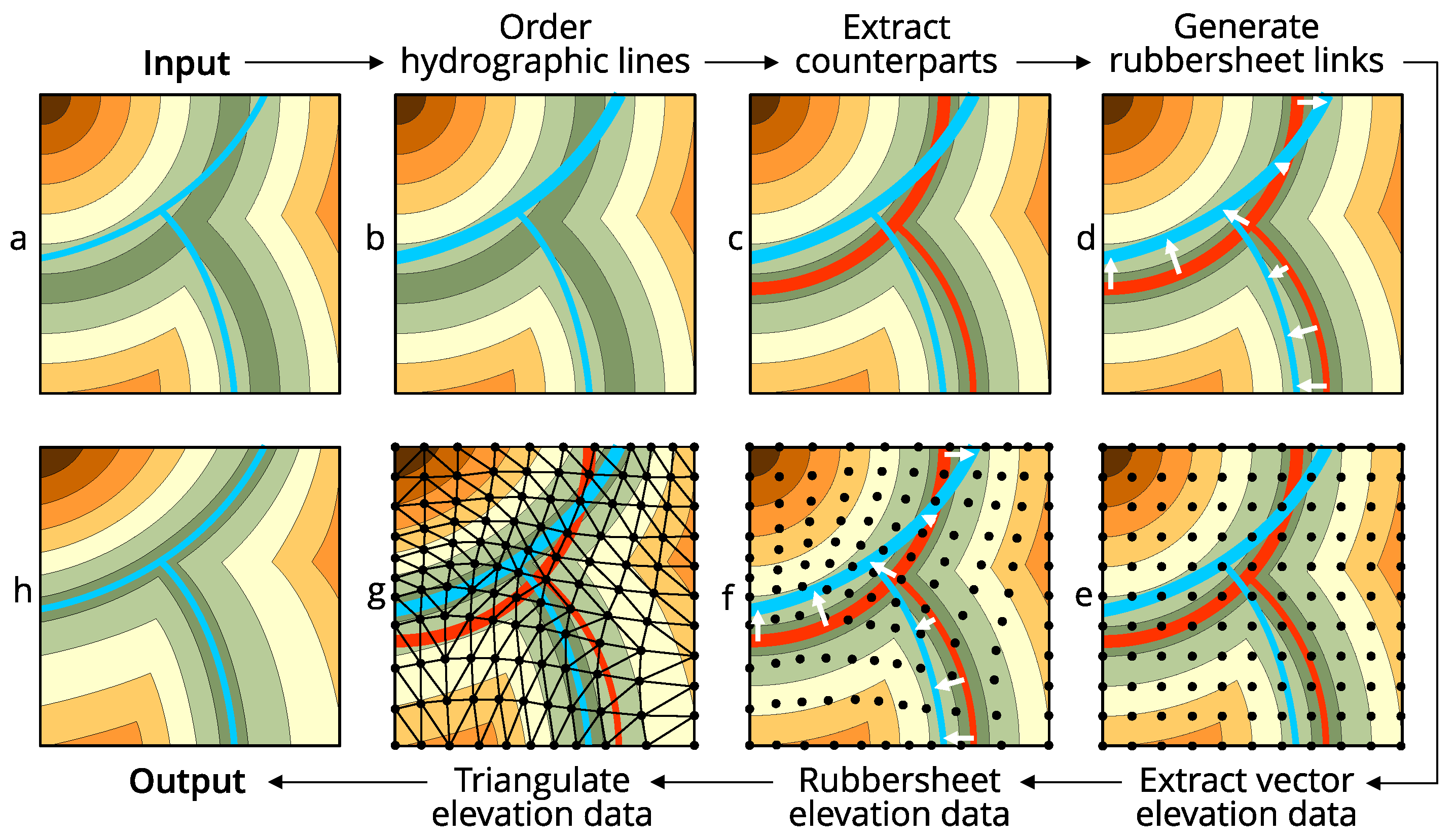
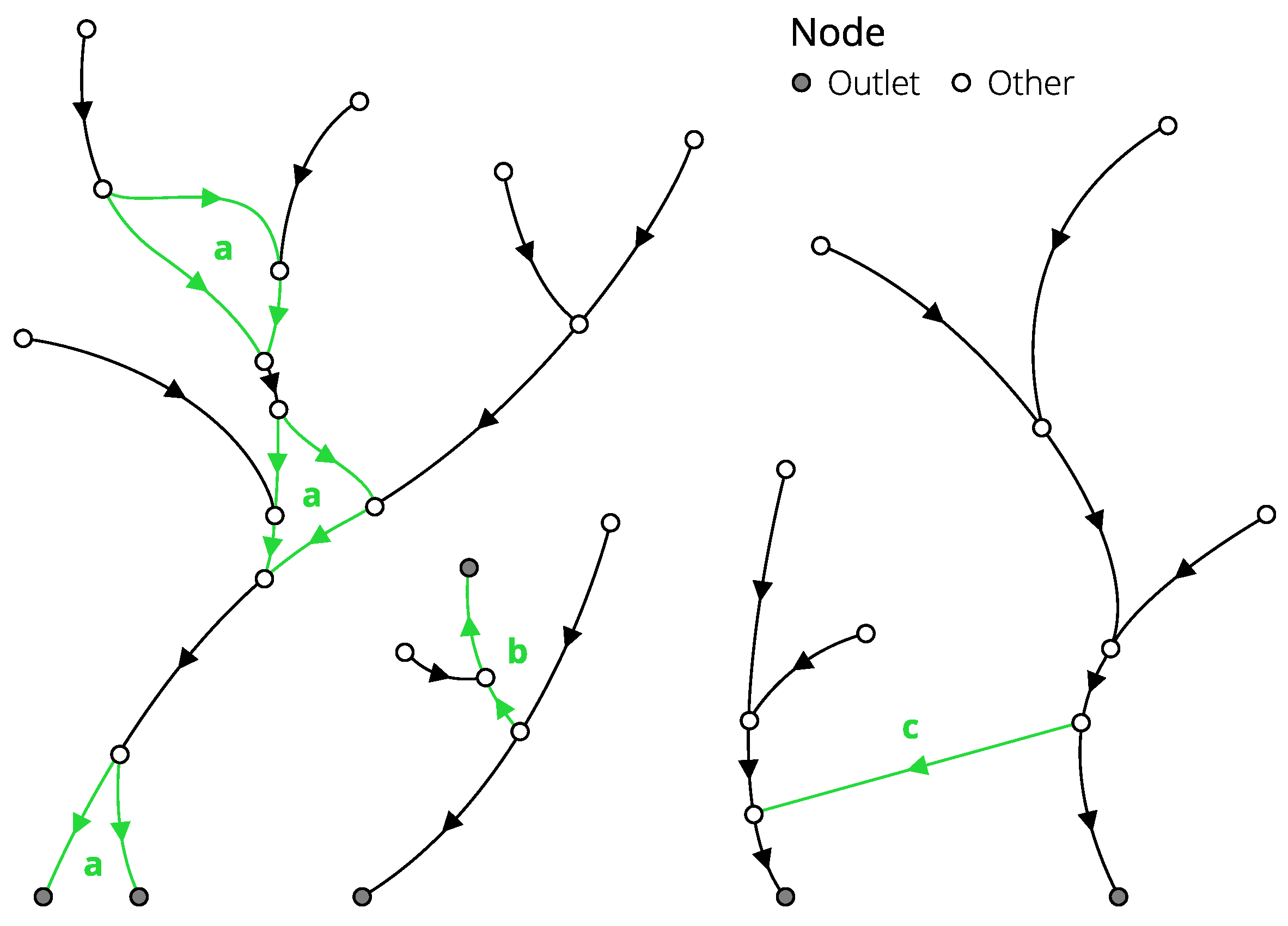
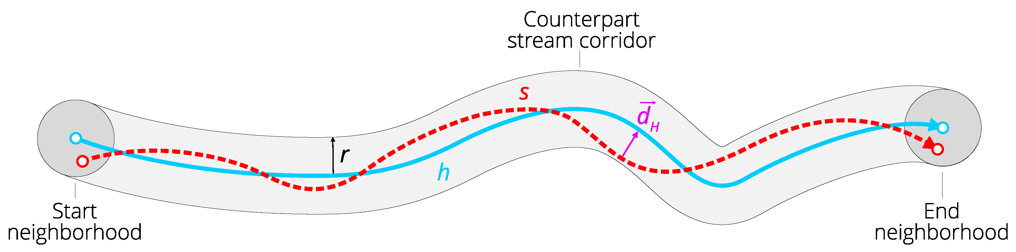
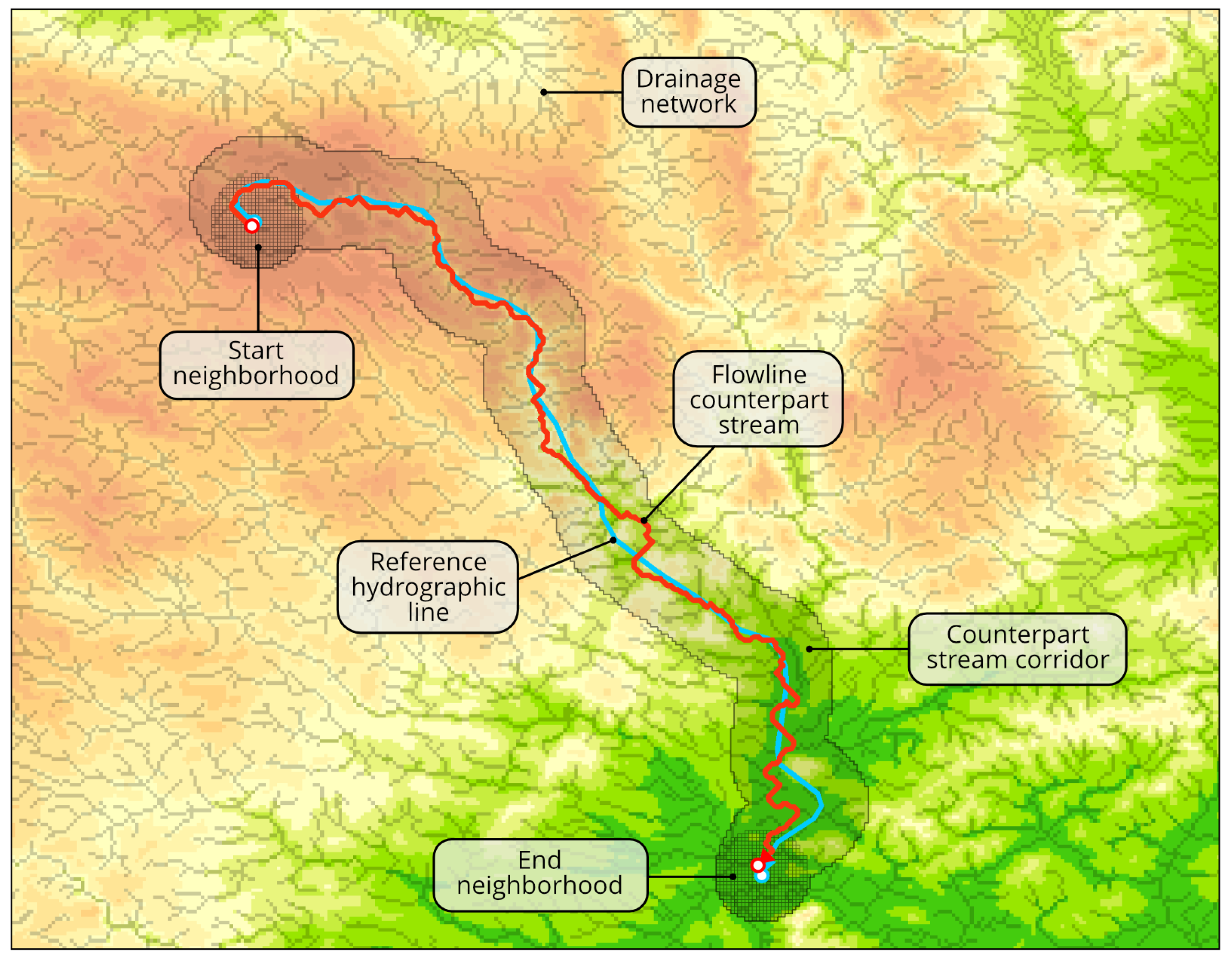
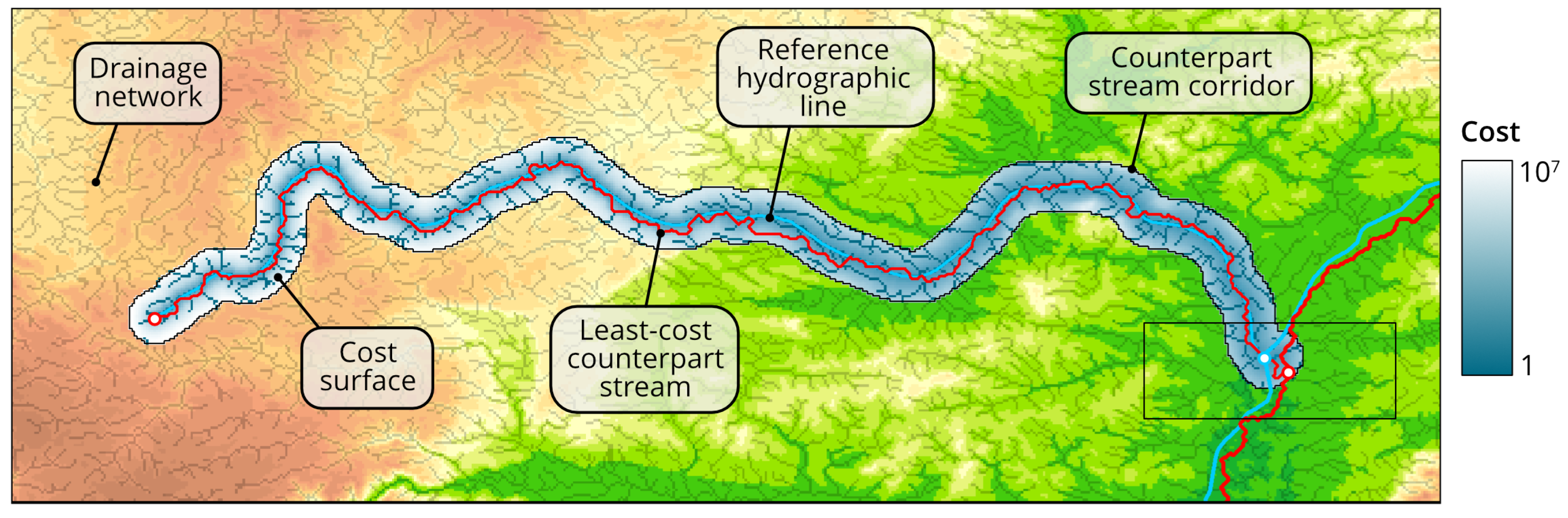
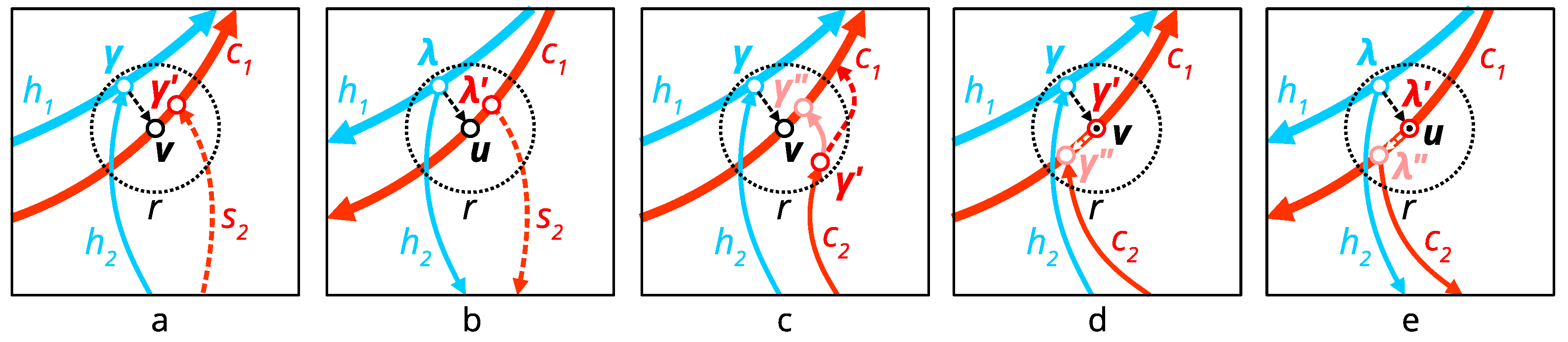
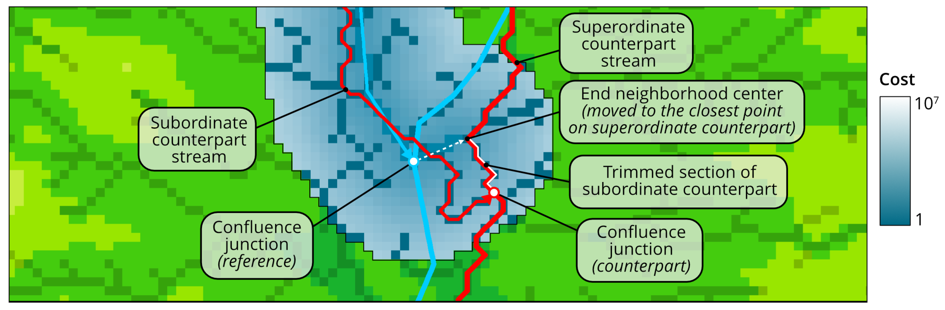
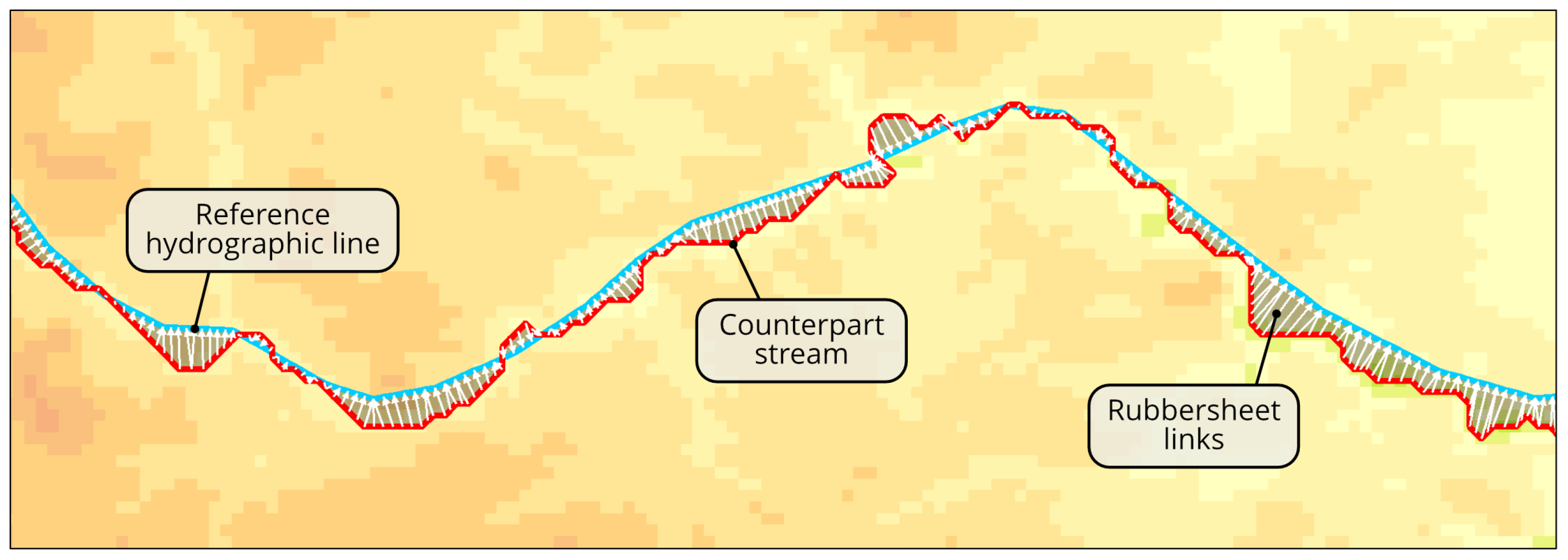
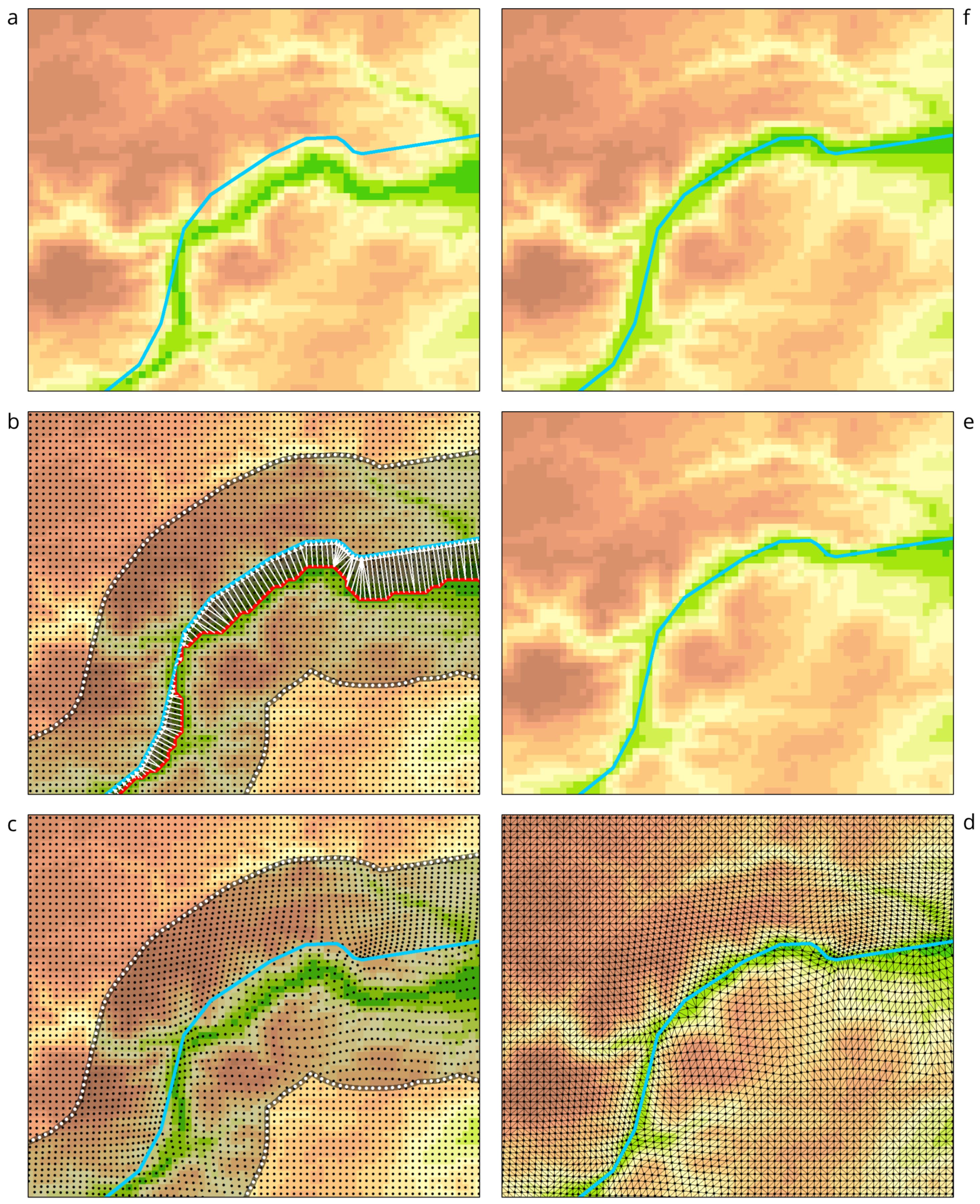
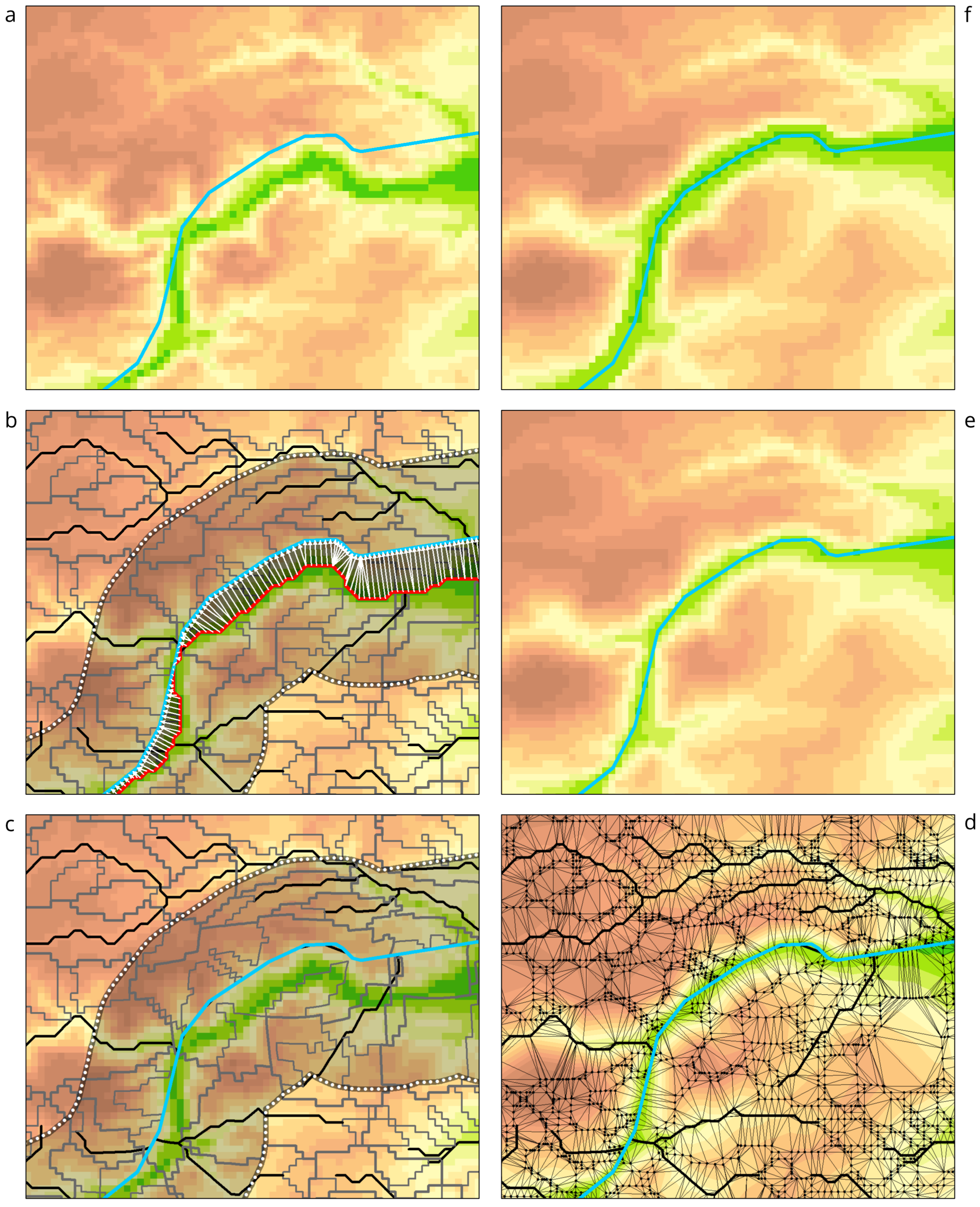
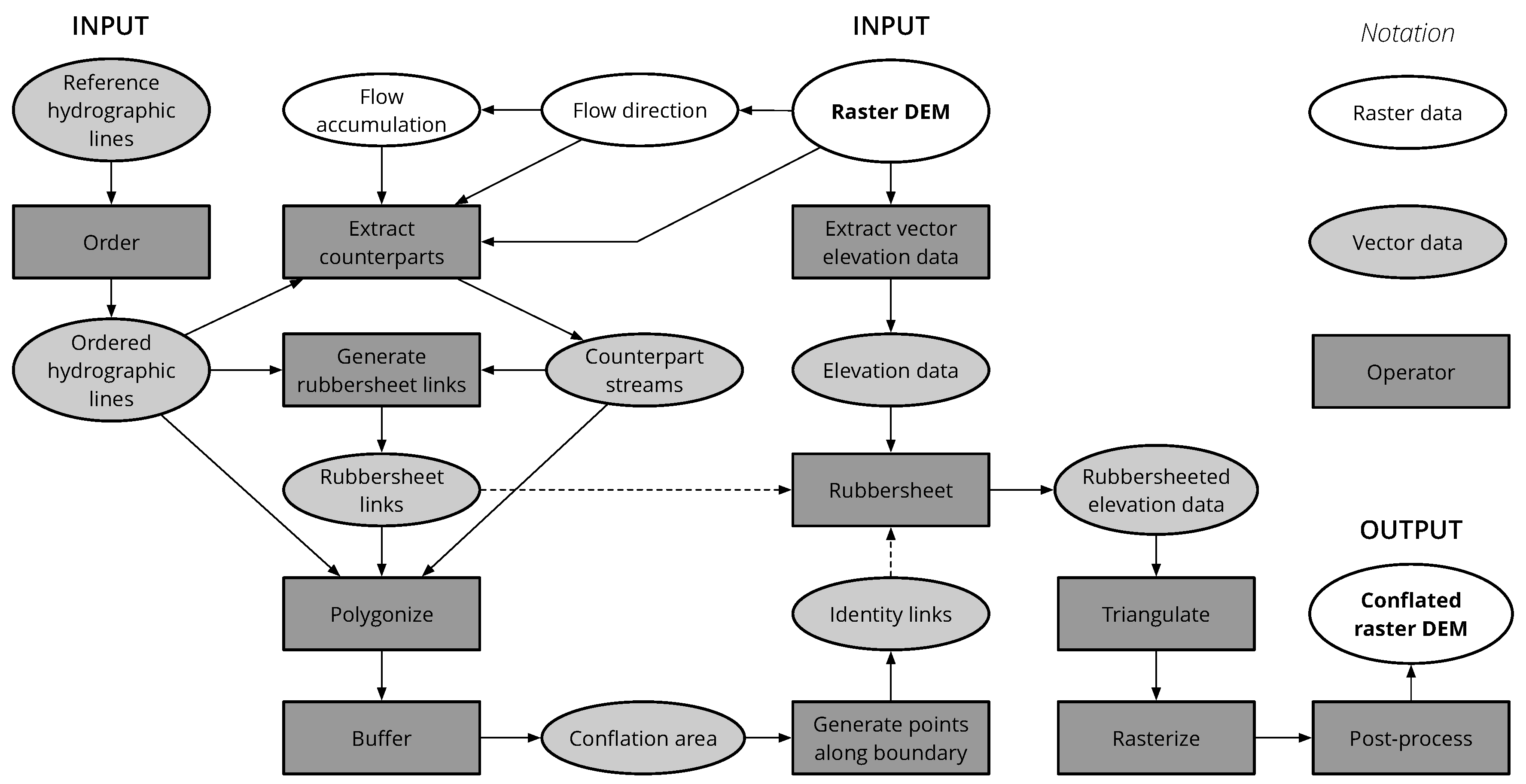
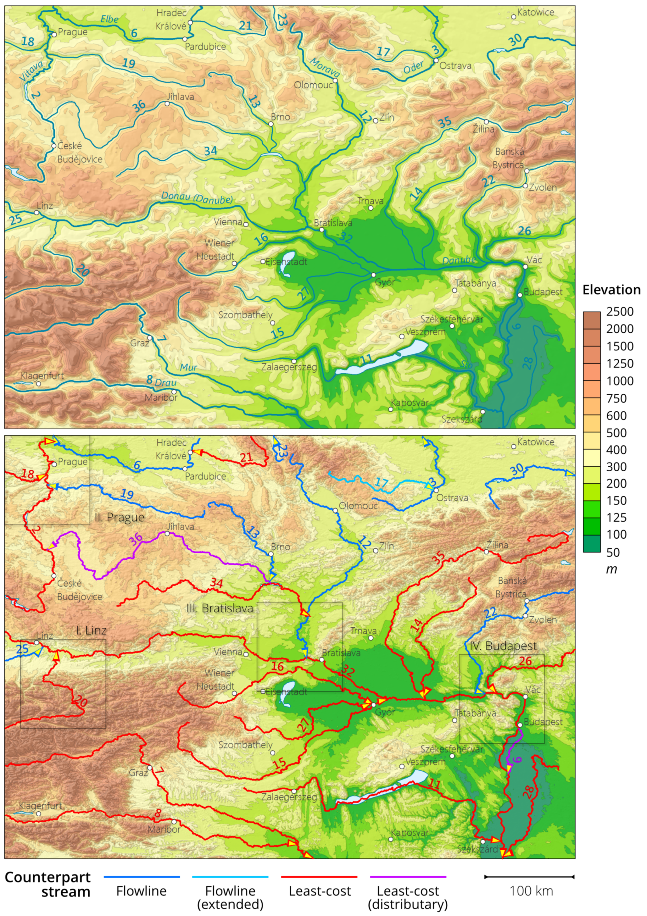
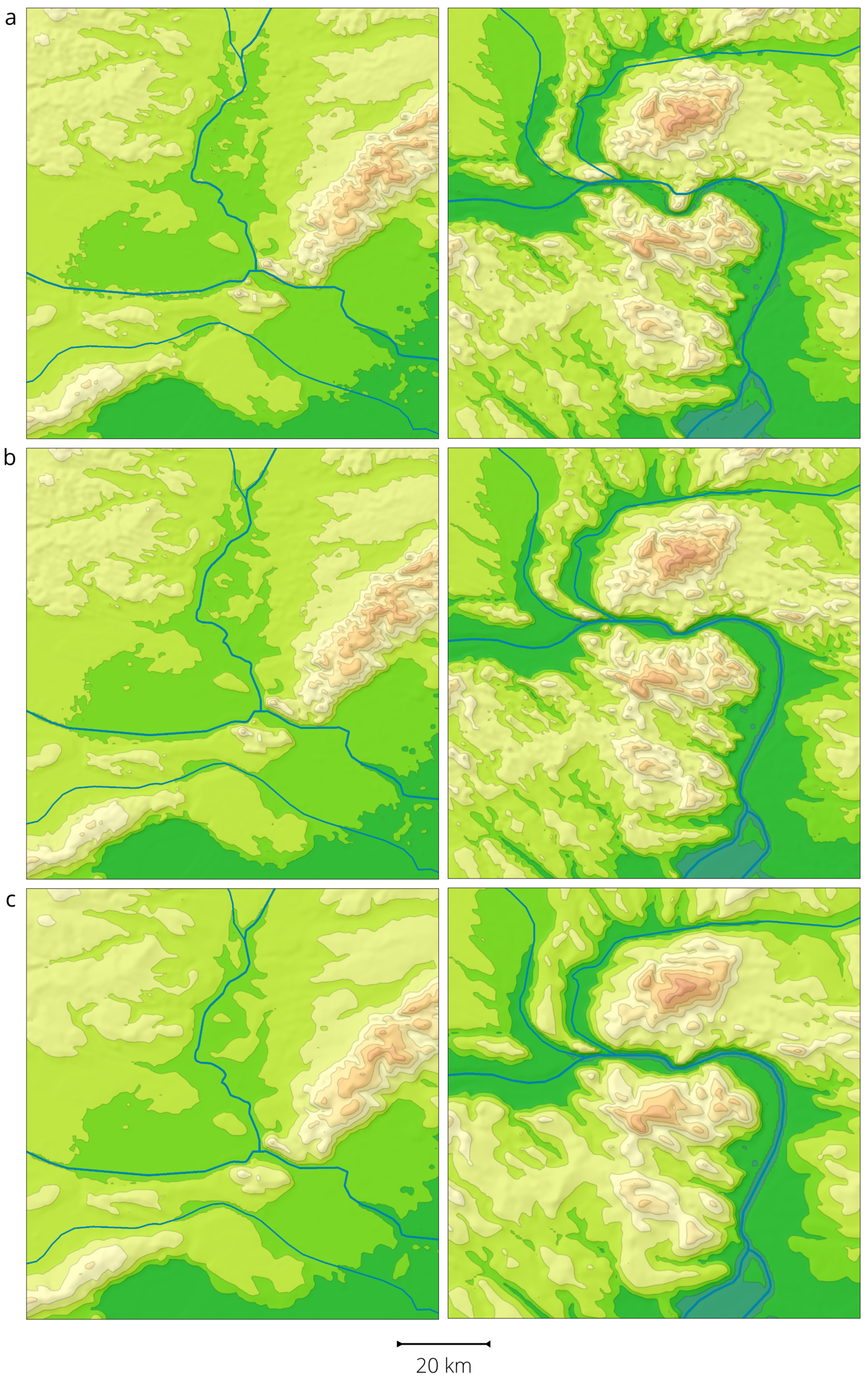
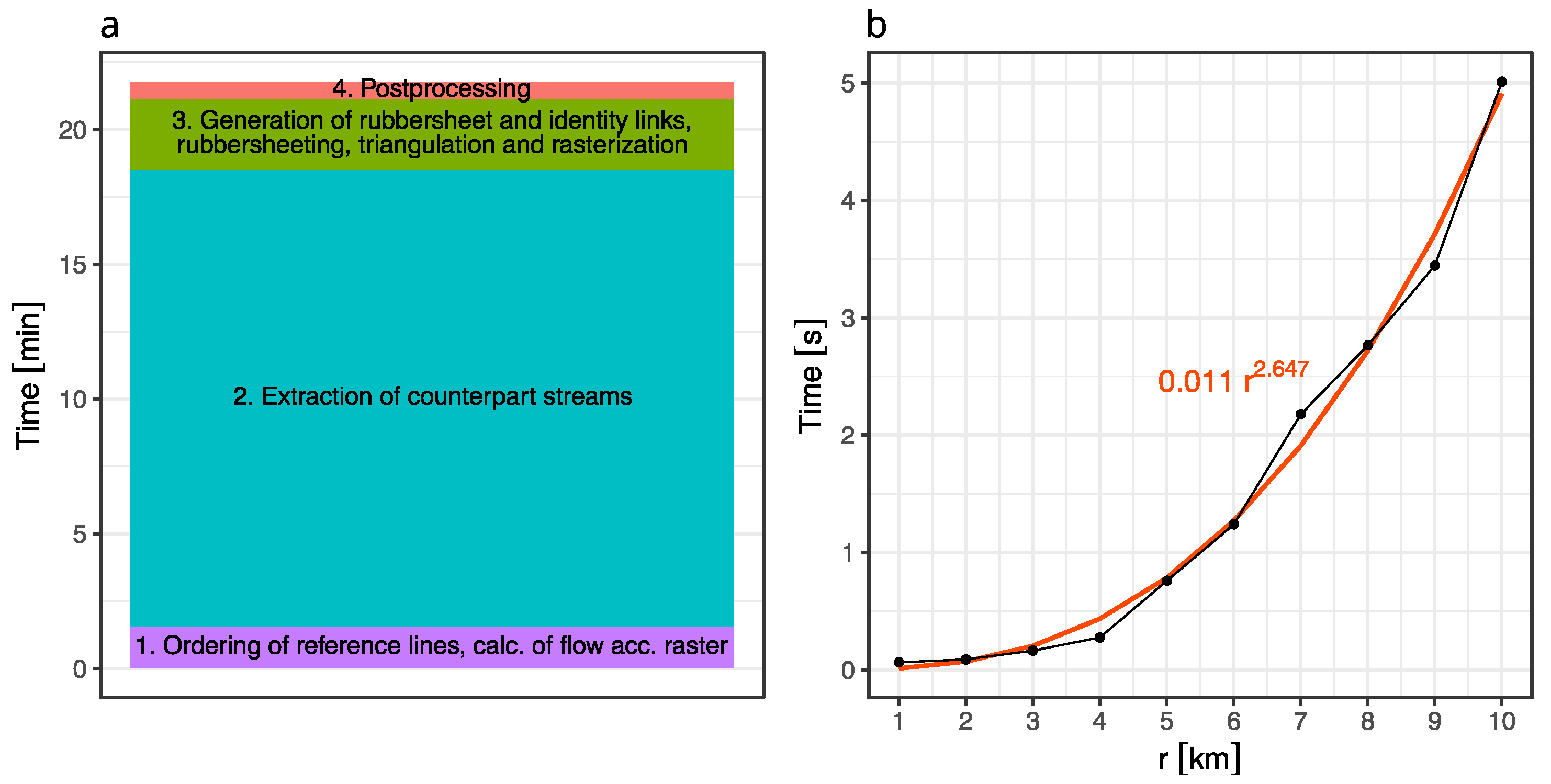
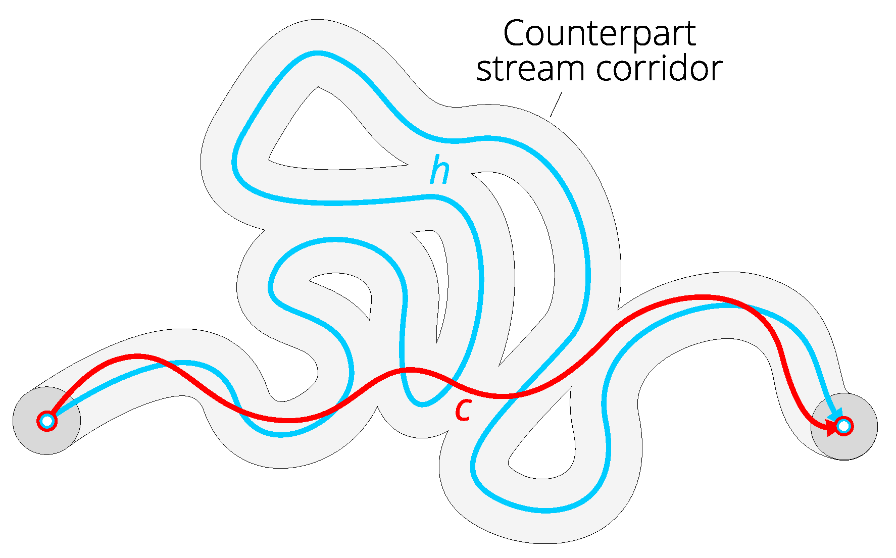
Table 1.
Attributes of ordered reference hydrographic lines.
| ID | CONFL | BIFUR | ITER | ORDER | TYPE |
|---|---|---|---|---|---|
| 1 | −1 | −1 | 1 | 1 | Main |
| 2 | −1 | 1 | 2 | 1 | Distributary |
| 3 | 1 | −1 | 2 | 2 | Main |
| 4 | 1 | −1 | 2 | 2 | Main |
| 5 | 1 | −1 | 2 | 2 | Main |
| 6 | 1 | 1 | 2 | 2 | Distributary |
| 7 | 4 | −1 | 3 | 3 | Main |
| 8 | 3 | 1 | 3 | 3 | Distributary |
| 9 | −1 | −1 | 1 | 1 | Main |
| 10 | −1 | 9 | 2 | 1 | Distributary |
| 11 | 10 | −1 | 3 | 2 | Main |
| 12 | −1 | −1 | 1 | 1 | Main |
| 13 | −1 | 12 | 2 | 1 | Distributary |
| 14 | 12 | −1 | 2 | 2 | Main |
| 15 | 12 | −1 | 2 | 2 | Main |
| 16 | 12 | −1 | 2 | 2 | Main |
| 17 | 14 | −1 | 3 | 3 | Main |
Table 2.
Summary of counterpart streams extraction results.
| ID | CONFL | BIFUR | ITER | ORDER | TYPE | COUNTERPART | , m | , m | , m | QUALITY |
|---|---|---|---|---|---|---|---|---|---|---|
| 2 | 6 | −1 | 2 | 2 | Main | Least-cost | 4065 | 4065 | 4065 | Strong |
| 3 | −1 | −1 | 1 | 1 | Main | Flowline | 3202 | 3202 | 3202 | Strong |
| 6 | −1 | −1 | 1 | 1 | Main | Flowline | 4412 | 4384 | 4384 | Strong |
| 7 | −1 | −1 | 1 | 1 | Main | Least-cost | 4705 | 4472 | 4472 | Strong |
| 8 | 7 | −1 | 2 | 2 | Main | Least-cost | 2809 | 2809 | 2809 | Strong |
| 9 | 32 | 32 | 2 | 2 | Distributary | Least-cost | 2357 | 2357 | 2356 | Strong |
| 11 | 32 | −1 | 2 | 2 | Main | Least-cost | 2375 | 2375 | 2375 | Strong |
| 12 | 32 | −1 | 2 | 2 | Main | Flowline | 5166 | 5136 | 5136 | Strong |
| 13 | 36 | −1 | 5 | 4 | Main | Flowline | 4586 | 4477 | 4477 | Strong |
| 14 | 35 | −1 | 3 | 3 | Main | Least-cost | 3307 | 3307 | 3307 | Strong |
| 15 | 32 | −1 | 2 | 2 | Main | Least-cost | 6264 | 6264 | 4277 | Weak |
| 16 | 15 | −1 | 3 | 3 | Main | Least-cost | 2884 | 2884 | 2884 | Strong |
| 17 | 3 | −1 | 2 | 2 | Main | Flowline | 4737 | 4737 | 4737 | Strong |
| 18 | 2 | −1 | 3 | 3 | Main | Least-cost | 2501 | 2501 | 1754 | Strong |
| 19 | 2 | −1 | 3 | 3 | Main | Flowline | 2510 | 2510 | 2510 | Strong |
| 20 | 32 | −1 | 2 | 2 | Main | Least-cost | 3341 | 3341 | 2581 | Strong |
| 21 | 6 | −1 | 2 | 2 | Main | Least-cost | 1987 | 1987 | 1987 | Strong |
| 22 | 32 | −1 | 2 | 2 | Main | Flowline | 4604 | 4604 | 4604 | Strong |
| 23 | −1 | −1 | 1 | 1 | Main | Flowline | 1378 | 1378 | 1378 | Strong |
| 25 | 32 | −1 | 2 | 2 | Main | Flowline | 2519 | 2519 | 2320 | Strong |
| 26 | 32 | −1 | 2 | 2 | Main | Least-cost | 4185 | 4185 | 4185 | Strong |
| 27 | 16 | −1 | 4 | 4 | Main | Least-cost | 4408 | 4408 | 4408 | Strong |
| 28 | 32 | −1 | 2 | 2 | Main | Least-cost | 2998 | 2998 | 2998 | Strong |
| 30 | −1 | −1 | 1 | 1 | Main | Flowline | 4059 | 4059 | 4059 | Strong |
| 32 | −1 | −1 | 1 | 1 | Main | Least-cost | 4206 | 4206 | 4206 | Strong |
| 34 | 12 | −1 | 3 | 3 | Main | Least-cost | 4417 | 4417 | 4417 | Strong |
| 35 | 32 | −1 | 2 | 2 | Main | Least-cost | 3689 | 3689 | 3689 | Strong |
| 36 | 2 | 34 | 4 | 3 | Distributary | Least-cost | 4032 | 4032 | 4032 | Strong |
Table 3.
Statistics of agreement between the reference hydrographic lines and the drainage network extracted from DEM.
Table 3.
Statistics of agreement between the reference hydrographic lines and the drainage network extracted from DEM.
| ID | ||||
|---|---|---|---|---|
| 2 | 0.758 | 0.015 | 0.991 | 0.003 |
| 3 | 0.830 | 0.018 | 0.992 | 0.004 |
| 6 | 0.560 | 0.024 | 0.993 | 0.003 |
| 7 | 0.415 | 0.018 | 0.998 | 0.001 |
| 8 | 0.457 | 0.021 | 0.966 | 0.006 |
| 9 | 0.433 | 0.047 | 1.000 | 0.000 |
| 11 | 0.620 | 0.018 | 0.992 | 0.003 |
| 12 | 0.396 | 0.022 | 0.998 | 0.002 |
| 13 | 0.577 | 0.029 | 1.000 | 0.000 |
| 14 | 0.539 | 0.026 | 0.977 | 0.007 |
| 15 | 0.457 | 0.021 | 0.982 | 0.005 |
| 16 | 0.382 | 0.024 | 0.929 | 0.010 |
| 17 | 0.470 | 0.033 | 0.977 | 0.008 |
| 18 | 0.549 | 0.050 | 1.000 | 0.000 |
| 19 | 0.509 | 0.027 | 1.000 | 0.000 |
| 20 | 0.463 | 0.027 | 0.985 | 0.005 |
| 21 | 0.646 | 0.030 | 1.000 | 0.000 |
| 22 | 0.567 | 0.024 | 0.997 | 0.002 |
| 23 | 0.591 | 0.059 | 0.978 | 0.015 |
| 25 | 0.862 | 0.031 | 0.877 | 0.030 |
| 26 | 0.621 | 0.030 | 1.000 | 0.000 |
| 27 | 0.513 | 0.026 | 0.993 | 0.004 |
| 28 | 0.553 | 0.028 | 1.000 | 0.000 |
| 30 | 0.820 | 0.021 | 0.964 | 0.010 |
| 32 | 0.449 | 0.013 | 0.997 | 0.001 |
| 34 | 0.589 | 0.021 | 0.994 | 0.003 |
| 35 | 0.484 | 0.018 | 0.958 | 0.006 |
| 36 | 0.556 | 0.019 | 0.985 | 0.004 |
Table 4.
Displacement statistics.
| Variable | Rubbersheet Links | Displacement Vectors |
|---|---|---|
| dx [m] | ||
| Mean (SD) | −49 (761) | −28 (397) |
| Median (Q1, Q3) | −16 (−302, 225) | −4 (−126, 92) |
| Range | [−5404, 6210] | [−4461, 3747] |
| dy [m] | ||
| Mean (SD) | 301 (926) | 179 (533) |
| Median (Q1, Q3) | 256 (−111, 803) | 98 (−22, 389) |
| Range | [−4675, 4390] | [−4675, 4390] |
| dxy [m] | ||
| Mean (SD) | 936 (808) | 467 (506) |
| Median (Q1, Q3) | 726 (334, 1259) | 302 (114, 643) |
| Range | [4, 6264] | [0, 5137] |
| dz [m] | ||
| Mean (SD) | - | 0.07 (13.77) |
| Median (Q1, Q3) | - | 0.03 (−1.52, 1.76) |
| Range | - | [−466.49, 390.49] |
| Total number | 22,606 | 393,622 |
© 2020 by the author. Licensee MDPI, Basel, Switzerland. This article is an open access article distributed under the terms and conditions of the Creative Commons Attribution (CC BY) license (http://creativecommons.org/licenses/by/4.0/).
Share and Cite
MDPI and ACS Style
Samsonov, T.E. Automated Conflation of Digital Elevation Model with Reference Hydrographic Lines. ISPRS Int. J. Geo-Inf. 2020, 9, 334. https://0-doi-org.brum.beds.ac.uk/10.3390/ijgi9050334
AMA Style
Samsonov TE. Automated Conflation of Digital Elevation Model with Reference Hydrographic Lines. ISPRS International Journal of Geo-Information. 2020; 9(5):334. https://0-doi-org.brum.beds.ac.uk/10.3390/ijgi9050334
Chicago/Turabian StyleSamsonov, Timofey E. 2020. "Automated Conflation of Digital Elevation Model with Reference Hydrographic Lines" ISPRS International Journal of Geo-Information 9, no. 5: 334. https://0-doi-org.brum.beds.ac.uk/10.3390/ijgi9050334
Note that from the first issue of 2016, this journal uses article numbers instead of page numbers. See further details here.