Construction, Detection, and Interpretation of Crime Patterns over Space and Time


1
College of Civil Engineering, Nanjing Forestry University, Nanjing 210037, China
2
National Engineering Research Center of Biomaterials, Nanjing Forestry University, Nanjing 210037, China
3
Key Laboratory of Virtual Geographic Environment, Ministry of Education, Nanjing Normal University, Nanjing 210046, China
4
Jiangsu Center for Collaborative Innovation in Geographical Information Resource Development and Application, Nanjing 210023, China
*
Author to whom correspondence should be addressed.
ISPRS Int. J. Geo-Inf. 2020, 9(6), 339; https://0-doi-org.brum.beds.ac.uk/10.3390/ijgi9060339
Submission received: 24 March 2020
/
Revised: 30 April 2020
/
Accepted: 25 May 2020
/
Published: 26 May 2020
(This article belongs to the Special Issue Urban Crime Mapping and Analysis Using GIS)
Abstract
:Empirical studies have focused on investigating the interactive relationships between crime pairs. However, many other types of crime patterns have not been extensively investigated. In this paper, we introduce three basic crime patterns in four combinations. Based on graph theory, the subgraphs for each pattern were constructed and analyzed using criminology theories. A Monte Carlo simulation was conducted to examine the significance of these patterns. Crime patterns were statistically significant and generated different levels of crime risk. Compared to the classical patterns, combined patterns create much higher risk levels. Among these patterns, “co-occurrence, repeat, and shift” generated the highest level of crime risk, while “repeat” generated much lower levels of crime risk. “Co-occurrence and shift” and “repeat and shift” showed undulated risk levels, while others showed a continuous decrease. These results outline the importance of proposed crime patterns and call for differentiated crime prevention strategies. This method can be extended to other research areas that use point events as research objects.
1. Introduction
Quantitative criminology has conducted an investigation into crime patterns. Crime pattern analysis uncovers the underlying interactive process between crime events by discovering where, when, and why particular crimes are likely to occur [1,2,3]. The outcomes improve our understanding of the dynamics of unlawful activities and can enhance predictive policing.
Early efforts found that crimes are not randomly distributed but tend to follow patterns. For example, researchers observed that disproportionate crimes occur shortly after the previous crimes and call this phenomenon repeat victimization [4,5,6,7]. In addition, many places exhibit similar crime distribution patterns due to their similar geographic features [8,9]. According to displacement or diffusion of benefits, nearby locations may experience repeated high crime risk due to the dynamic nature of criminal opportunities [10,11,12,13,14,15,16,17]. Many studies have been conducted to detect and interpret these phenomena [4,5,6,7,8,9,10,11,12,13,14,15,16,17,18,19,20,21,22]. However, they are typically designed to investigate one particular pattern type and often overlook the complexity of crimes [17]. Crime changes across space, time, and culture [23,24]. Moreover, they are not generalized enough to detect, display, and interpret combinations of those patterns simultaneously.
Considering the complexity of crimes, we must study a comprehensive model. Utilizing graph representation, we can efficiently and effectively discover crime patterns, including repeat and near-repeat (RNR) co-occurrence, and geographic shift. Besides, we will introduce and study a combination of these patterns. Compared to previous studies, we aim to detect, demonstrate, and analyze crime relations that have not been studied yet. The research results are expected to improve crime research and analysis by providing multiple crime patterns. This method can be extended to other research areas that use point events as research objects.
2. Literature Review
Crimes are often linked because of their similarities [25,26,27]. The same offenders commit some crimes, while others occur in similar places. For offenders, these places provide suitable opportunities because they can replicate their experience from previous crimes and reoffend after rational consideration of risks and rewards [28,29]. The literature suggests that these linked crimes are usually similar to each other in nature [21,30].
Crime pairs committed in close proximity within a short time are known as repeats and near-repeats (RNR) [25]. Two hypotheses could account for such phenomenon: “boost” and “flag” [4,6,7,13,17,19,21,31,32,33,34,35,36]. The boost theory explains that an initial crime can boost the risk of subsequent victimizations [19,32,34]. Offenders may gain experience from a previous offense or gain information from other offenders and commit another crime at the same or proximate place [37]. In this situation, previous victimizations “boost” future crimes. Flag theory argues that opportunistic offenders may flag certain vulnerable objects as targets [19]. These targets may be physically soft or not well protected with security controls [4,18,19,37]. Thus, future offenders can take advantage of these flagged places and repeatedly commit crimes. Both boost and flag theories account for crime pairs close in space and time.
Shift is an extended pattern of near-repeat. While RNR focuses on spatial-temporally close crime pairs, shift patterns emphasize crime pairs close in time [11,14,15,16,17,29,38,39]. This phenomenon could be interpreted as a response to crime prevention initiatives [14,16,17]. When one place has been victimized, motivated offenders would displace to alternative places for suitable opportunities [29]. Further interpretation could be found in crime pattern theory and routine activity theory [1,2,22,40,41,42,43,44,45]. According to these theories, people participate in routine activities between geographic nodes, such as homes, workplaces, and entertainment sites. Over time, they get better acquainted with the places and form their own awareness space, also known as “mental maps” [29,42]. When one opportunity disappeared, the motivated offenders would navigate to other places on their “mental map” to explore alternative opportunities, even those opportunities can be far away. As such, two places may experience a high crime risk consecutively due to their similar geographic characteristics [17]. As such, the links between crime pairs are critical for understanding criminal activities. Identification of this pattern could uncover place pairs rich in crime shifts.
Crimes could be linked when they were committed at the same/close time [8,9]. Research shows that many facilities may report similar crime patterns due to their geographical features [22,40]. For example, bars, entertainment sites, and liquor stores may attract a large number of people on certain days like weekends and game days [46]. These facilities usually demonstrate uniform opening time and may attract similar groups of people [47]. Criminal opportunities can be created during shared opening times and activities (e.g., sports events). When converged with suitable targets, along with the absence of guardianship, a motivated offender may commit crimes and thereby form co-occurring crimes [43]. The linked crime pairs typically inform similar crime patterns at/around certain geographic facilities [8,9]. Identifying this pattern would be beneficial for discovering places that are typically attractive for certain crimes.
Measurements of the patterns vary significantly. The Knox test is typically adopted to test RNR, while the weighted displacement quotient is applied to measure crime shift [14,21,48]. More recently, data mining methods with frequent item mining have been applied to detect frequent co-occurring crime pairs [8,9]. However, these mathematical methods were typically designed for one pattern measurement. We must investigate a generalized model for combinations of these models.
Graph theory has been applied in many research fields. According to this theory, a graph can represent a group of spatial-temporal events that consist of nodes and edges. Nodes and edges represent the events and their associations, respectively. For a crime network, the edges represent the interactive relationships between crime events. A recent study applied graph theory to the analysis of crime patterns and relationships within hotspots [49,50]. Nevertheless, the graphs were constructed based on the geometric characteristics of crime events and are difficult to explain using criminology theories. Furthermore, the research was restricted to a certain space time scale. Our current research will construct graphs based on existing criminology knowledge and analyze patterns on different scales. The research results can reveal the complex interactive relationship between crimes and are expected to benefit our understanding of the dynamic nature of crimes.
3. Methodology
In this study, we introduce three basic crime patterns as well as four combinations of these patterns. The Monte Carlo simulation method will be introduced to identify statistically significant crime patterns. Finally, we will display and analyze the experimental results.
3.1. Event Network
According to graph theory, nodes and edges make up a graph. In this study, a crime network is composed of crime events, indexed by i, and the links between each crime pair. Each of the crimes was recorded with geographical location, , and time of occurrence, . The shorthand represents the spatial and temporal distances between crime pairs , which can be calculated with the following equation:
The nodes and edges construct a spatial-temporal network in which two crimes can be connected if the spatial distance and/or temporal distance is smaller than specified thresholds , respectively. In order to detect crime patterns on multiple scales, the spatial and temporal thresholds are empirically determined at space-time scales with a difference of 200 m and seven days, respectively. Manhattan distance is adopted for this research because it follows a grid-like path, which approximates the actual path between points people travel along in the urban context [51]. Previous studies have shown statistically significant relationships between burglaries that occur close together spatially and temporally [4,6,20,52]. Therefore, burglary is selected as the research object in this study.
3.2. Crime Patterns and Crime Networks
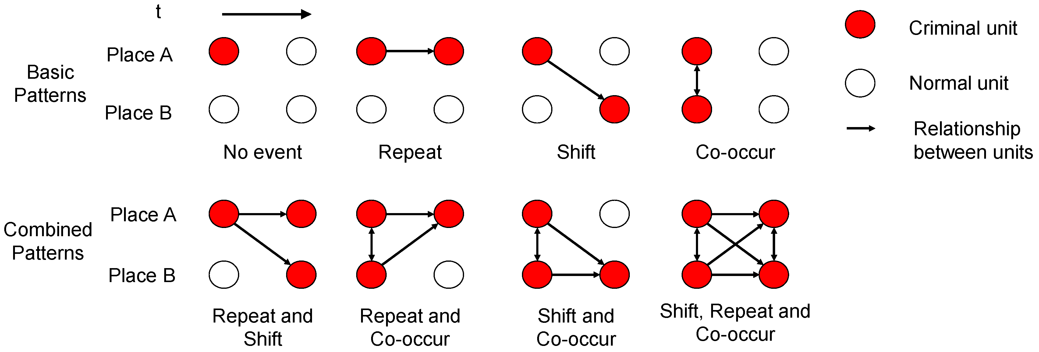
With the basic crime patterns, we construct three basic crime patterns as well as combinations of these patterns (Figure 1, Table 1). The three basic patterns include RNR, shift, and co-occurrence (the subgraphs in 1st row of Figure 1). The four combined patterns are composed of basic patterns, which represent more complex crime associations (the subgraphs in 2nd row of Figure 1).
In Figure 1, the horizontal axis is the time dimension (Figure 1, Table 1). As such, the “repeat” graph represents the phenomenon in which two crimes occur one after another in the same place. The “shift” graph represents two crimes committed consecutively at two different places. The “co-occurrence” graph represents two simultaneous crimes committed at two different places. It is necessary to note that near-repeat will be detected together with a shift even though they represent two distinct phenomena [6,21,32]. As such, geographic shift refers to displacement/deflection and near-repeat. Displacement/deflection cannot be separated from near-repeat as it is difficult to determine why the following crime geographically shifted as of the initial crime [10].
Repeat and shift is a combination of repeats and shifts. When one crime is committed in property A, another crime will be committed at properties A and B. Repeat and co-occurrence is a combination of the two. Two places were victimized at the same time. One of the two places experienced another crime shortly after the previous. Shift and co-occurrence are essentially the same as repeat and co-occurrence. Therefore, only one of the two patterns is calculated. The last pattern is shift, repeat, and co-occurrence. It can be interpreted as two co-occurring crimes, followed by two others shortly after.
Considering the various risk levels introduced by the research results on RNR, the interactive relations show various intensities on different space-time scales [6,7,17,20,21,35]. Therefore, the spatial and temporal thresholds are empirically determined at space-time scales with a difference of 200 m and seven days, respectively. Given the thresholds, the spatial-temporal networks for each pattern are constructed in the following steps.
3.3. Crime Risk Introduced by the Crime Patterns
Monte Carlo simulation was conducted to estimate the risk level introduced by each crime pattern. First, the crime pairs satisfying the definitions of crime patterns were connected and marked as subgraphs (Table 1). Then, the number of each crime pattern was counted according to its corresponding space-time band. At last, the count of patterns from real crime data was compared against the expected counts generated by simulated data.
In this calculation, a connection between one pair of crime represents their distance over space and time. Therefore, the ratio of the actual number of patterns against all expected numbers of patterns in simulated data can statistically show the risk level R introduced by crime patterns.
Higher values mean higher risk levels introduced by one pattern, while lower values mean lower risk levels introduced by one pattern. The significance level of a risk value is determined by the percentile level of the number of observed crime patterns in the counts of simulated crime patterns.
For each pair of crimes, three basic patterns are first detected. If two crimes are at the same location, then the two crimes can be connected as a subgraph for repeat pattern. If two crimes are committed at the same time but located at different places, then the two crimes are connected as a subgraph for co-occurrence pattern. Similarly, if two crimes are located at two different places, the earlier one has no following crime committed at the same place, while the latter has no previous crime at the same place. Then, this pair of crimes can be connected as a subgraph for shift pattern.
Following the basic patterns, we further detect their combinations. The repeat and shift pattern can be detected when a repeat occurs and one crime is committed at another place as a shift. A repeat and co-occurrence pattern can be detected when a co-occurrence occurs and one crime is committed after one of the two co-occurring crimes. A repeat, shift, and co-occurrence pattern can be detected when a co-occurrence takes place and two crimes are committed after the two co-occurring crimes, respectively. Crime simulation and risk calculation are completed on Matlab platform.
4. Study Area and Data
Complying with the confidentiality requirements of the local Public Security Bureau (PSB), we adopted the short-term N to represent large Chinese cities. According to data from local demographic departments, 2.6 million permanent residents and 0.7 million migrants live in the study area [53]. The registered unemployment rate for N city is 1.82% and the total administrative area includes 4 districts, covering 266 km2.
At the beginning of the 21st century, N city experienced a period of rapid economic development. Like many other cities in China, ancient buildings at the central part were well kept as city features, while many new communities were built in the suburban areas for urbanization. Besides, the local public transportation system was constructed to improve the efficiency of transport for citizens.
The dataset adopted for this research contains the location and date of the crime records. Previous studies have shown statistically significant relationships between burglaries that occur close together spatially and temporally [4,20,52]. Therefore, burglary is selected as the research object in this study. After being registered on the map, 8561 burglaries with coordinates and date were used for the current research. These crime records were between January 2013 and December 2013.
Community sizes and population density vary across N city, which is quite similar to the study area used in existing Chinese research [50]. Combined with the other result from western countries, we chose a 200 m spatial bandwidth, a seven-day temporal bandwidth.
5. Experimental Results
Following the crime patterns in Table 1, we constructed the corresponding networks. Figure 2 represents the results of pattern analysis. The value in each cell informs the crime risk level over an expected frequency in the corresponding spatial-temporal bands. Dark units correspond to larger values and inform higher crime risk, while light-colored units correspond to smaller values and inform lower crime risk. White units correspond to insignificant values.
As shown in the figures, the burglary risk level introduced by the patterns varies a lot (Figure 2). As a classic pattern, the “repeat” phenomenon is observed to exhibit within 49 days. The highest risk level is located between eight to 14 days of bandwidth. The ‘co-occurrence’ phenomenon is observed to exhibit within 200 m. Therefore, the frequency of co-occurrent crimes within 200 m is significantly greater than expected. Only one significant cell value was observed in the figure “shift”, which indicates that the “shift” pattern is significantly more frequent than expected. Once a location experiences a burglary, the chance of the second one taking place within one to 200 m and within the next seven days is significantly greater than if there were no discernible patterns (Figure 2).
According to the definition of the “repeat and shift” pattern, once a place was victimized, the possibility for both the same place and nearby places within 1000 m to experience another victimization is significantly high. Cells within 200 m and seven days exhibit high crime risk, which indicates that both the previous victimized places and their neighbors within 200 m and seven days would experience high crime risk, respectively (Figure 2).
The figure ‘co-occurrence and shift’ in Figure 2 shows the crime risk informed by “co-occurrence” and the shift pattern. According to the definition of this pattern, once two adjacent places simultaneously experienced crimes, the possibility for one to experience another crime is significantly high. Values were observed within 1000 m and 35 days (Figure 2). The highest value is located at “1–200” meters and “1–7” days cell, which indicates that the risk level within the corresponding spatial-temporal area is the highest one than expected.
The figure ‘Co-occurrence, repeat, and shift’ in Figure 2 indicates the crime risk informed by the co-occurrence, repeat, and shift patterns. This graph shows an elevated burglary risk in the 0–600 m spatial range and within 49 days informed by co-occurred burglaries. The cell values within 0–14 days and 0–200 m are much higher than the other cell values, and a much higher crime risk level could be expected for this pattern. Many of the patterns showed significantly elevated burglary risk within 200 m and 14 days after the original events. This space-time range is consistent with previous research results using burglary data in China. The risk would decrease to normal over space and time.
Some of the patterns show higher burglary risk levels, while others show lower. The combined patterns estimate a higher risk than the basic patterns. Therefore, crimes are more likely to occur in clusters than in pairs. The most complicated pattern co-occurs, and repeat and shift patterns could estimate the highest risk level (>6), which means this pattern may have a better ability to predict crime risk than others. The repeat pattern performs the lowest risk level.
6. Analysis
This study applied graph theory to a burglary dataset and focused on analyzing the potential ability of crime patterns represented by subgraphs to elevate crime risk. Finally, we statistically confirmed the proposed patterns. At least in N, a large Chinese city, the burglary data shows significant risk level over space and time with respect to the proposed patterns. On linking the crimes into subgraphs, the patterns revealed that the heightened risk created by a previous burglary event remained within a limited area in space and time.
Consistent with previous literature, the results show that the repeat phenomenon is evident for burglary in a Chinese context [6,7,17,35,36,50,54]. The elevated risk level was statistically significant at 49 days. This continuous high crime risk can lead to hotspots, which call for preventive police deployment at the repeatedly victimized places. According to the “flag” hypothesis, these places have disadvantages that attract people’s attention and provide opportunities for offenders [19]. Thus, some special maintenance is necessary to eliminate these disadvantages.
Compared to the other patterns proposed in this approach, however, the repeat pattern creates the lowest risk level. Given this result, the traditional crime prediction method, which gives equal weight to recent crime events, may overlook the potential ability of historical crimes for crime prediction [34,55,56]. Separating crimes based on their patterns may help develop crime prediction methods and improve their efficiency.
A shift pattern was observed and statistically significant within a limited spatiotemporal range of 200 m and seven days. As mentioned, we hypothesize this pattern to be composed of several phenomena, such as displacement, diffusion, and near repetition. In the literature, displacement and diffusion were observed to occur in a much larger spatiotemporal area. For example, Wang and Liu observed significantly elevated burglary risk within 600 m and 28 days [17]. Ratcliffe and Breen quantitatively measured displacement over 1 mile [14,57]. However, the elevated risk area created by the shift pattern is very limited. This result suggests that burglars are likely to transfer to proximate places for other opportunities, while there are no co-occurrences or repeats occur. Such small impact areas suggest that the “shift” pattern is more likely to be composed of near-repeat rather than displacement.
The co-occurrence phenomenon can be interpreted in two ways. First, similar places were hypothesized to share similar geographic features, which can exert similar impacts on people and, therefore, produce the same opportunities for these places on the same day [9]. This interpretation emphasizes the shared vulnerability of the co-victimized objects as a key reason for the co-occurring victimization. Second, many crimes that occur in proximity and on the same day are usually serial crimes. Offenders may commit two burglaries consecutively on the same day just because the second victim seems as vulnerable as the first one. The first account emphasizes the impact of criminogenic facilities, while the second one argues for the disadvantages within neighborhoods. The experimental results suggest that co-occurred crimes take place within a limited space area. These criminogenic places require proactive measures to prevent more crimes.
Compared to basic patterns, joint patterns create higher risk levels, which further outlines the importance of crime patterns. At least in this case study, crimes tend to occur in forms of complex patterns rather than simple ones. These influential patterns are more likely to form hotspots than crime pairs.
The influence of joint patterns differs in terms of intensity and scope. The crime risk generated by repeat and shift patterns ranges from 49 days to 1000 m. Furthermore, the risk level was not linearly decreased but showed some fluctuation, which suggests periodic activities or displacement of offenders [6]. Co-occurrence and shift patterns create linearly decreased crime risk where the highest burglary risk is directly after the origin crime in this pattern. Once a co-occurred crime was committed, the proximate areas would experience high crime risk within seven days. The burglary risk decreases rapidly after seven days. Similarly, co-occurrence, repeat, and shift patterns create a highly elevated crime risk level within 200 m and 14 days as well as a rapidly decreased risk level outside the range. The heightened crime risk within a limited area is more likely to be interpreted as a result of the attractiveness of specific geographical characteristics for potential offenders [19,32,34].
The distinct risk patterns suggest different levels of crime prevention measures and crime prediction methods. For example, repeat and shift patterns create an undulated crime risk within 1000 m and 49 days of space and time. As such, crime prevention initiatives must consider special strategies to decrease crime risk in specific locations over short periods. In contrast, the other two patterns seem to generate a high level of risk directly after the original crime. The two patterns call for preventive measures immediately after the original crime.
7. Conclusions
In this study, graph theory was introduced to construct crime graphs. Several subgraphs were generated to represent the complex interactive relationships between crimes. Using the burglary record from a large Chinese city, crime patterns were statistically significant within a certain spatiotemporal bandwidth. The identification of these patterns further confirmed the interactive associations between crimes.
According to graph theory, the subgraphs were created based on space-time distances between crimes. These subgraphs expanded the repeat and near-repeat phenomena with more crime patterns. The experimental results demonstrated the undulation of risk after a previous burglary and displayed how crimes would occur according to these patterns. Further, the differences among crime risks introduced by different patterns are also noteworthy. They show that the subgraphs guided by graph theory can help classify crime patterns and benefit crime risks introduced by these patterns.
The basic crime patterns create a relatively low burglary risk as of the combined crime patterns. Co-occurring patterns suggest special maintenance performed for the vulnerable neighbors. Shift patterns call for preventive measures at places nearby the previous crime locations. The complex patterns generate a higher risk level than the basic patterns. Repeat and shift patterns create undulated burglary risk, which calls for periodic preventative activities at special times and places. The other combined patterns, however, generate high crime risk within a limited spatiotemporal area. Proactive policing is necessary shortly after the original crimes to prevent crime and reduce overall crime levels.
Given the various range and intensity levels of crime risk, crime pattern analysis can be applied to improve crime prediction accuracy and increase efficiency of patrols. The modified method and the introduced patterns could be applied in point-event-based studies.
The current research is limited to discerning the social environmental characteristics of the proposed patterns. These patterns may be associated with different social environmental characteristics. Identifying the criminogenic factors for these patterns is critically important for developing crime prevention strategies. For example, neighbors with co-occurred crimes may expose similar vulnerabilities offenders. Identifying the criminogenic factors for these patterns can reveal why these patterns form at certain places.
Author Contributions
Formal analysis, Zengli Wang; methodology, Zengli Wang; visualization, Zengli Wang; writing—original draft, Zengli Wang; writing—review and editing, Hong Zhang. All authors have read and agreed to the published version of the manuscript.
Funding
This research was funded by the National Natural Science Foundation of China (No. 41501488).
Acknowledgments
The authors would like to acknowledge the Public Security Bureau of N city for providing the crime data. The authors also thank the reviewers for their constructive comments and suggestions that improved the quality of this paper.
Conflicts of Interest
The authors declare no conflict of interest.
References
- Brantingham, P.J.; Brantingham, P.L. Environmental Criminology; Sage Publications: Beverly Hills, CA, USA, 1981. [Google Scholar]
- Brantingham, P.J.; Brantingham, P.L. Crime pattern theory. In Environmental Criminology and Crime Analysis; Wortley, R., Mazerolle, L., Eds.; Willan: Cullompton, UK, 2008; pp. 78–93. [Google Scholar]
- Brantingham, P.; Brantingham, P. Crime pattern theory. In Environmental Criminology and Crime Analysis; Willan: Cullompton, UK, 2013; pp. 100–116. [Google Scholar]
- Johnson, S.D. Repeat burglary victimisation: A tale of two theories. J. Exp. Criminol. 2008, 4, 215–240. [Google Scholar] [CrossRef]
- Glasner, P.; Johnson, S.D.; Leitner, M. A comparative analysis to forecast apartment burglaries in Vienna, Austria, based on repeat and near repeat victimization. Crime Sci. 2018, 7, 9. [Google Scholar] [CrossRef]
- Wang, Z.; Liu, X. Analysis of burglary hot spots and near-repeat victimization in a large Chinese city. ISPRS Int. J. Geo-Inf. 2017, 6, 148. [Google Scholar] [CrossRef] [Green Version]
- Wang, Z.; Zhang, H. Understanding the spatial distribution of crime in hot crime areas. Singap. J. Trop. Geogr. 2019, 40, 1–14. [Google Scholar] [CrossRef]
- Mohan, P.; Shekhar, S.; Shine, J.A.; Rogers, J.P. Cascading spatio-temporal pattern discovery. IEEE Trans. Knowl. Data Eng. 2011, 24, 1977–1992. [Google Scholar] [CrossRef] [Green Version]
- Shekhar, S.; Mohan, P.; Oliver, D.; Zhou, X. Crime Pattern Analysis: A Spatial Frequent Pattern Mining Approach; University of Minnesota: Minneapolis, MN, USA, 2012; p. 41. [Google Scholar]
- Barr, R.; Pease, K. Crime placement, displacement, and deflection. Crime Justice 1990, 12, 277–318. [Google Scholar] [CrossRef]
- Bowers, K.J.; Johnson, S.D. Measuring the geographical displacement and diffusion of benefit effects of crime prevention activity. J. Quant. Criminol. 2003, 19, 275–301. [Google Scholar] [CrossRef]
- Guerette, R.T.; Bowers, K.J. Assessing the extent of crime displacement and diffusion of benefits: A review of situational crime prevention evaluations. Criminology 2009, 47, 1331–1368. [Google Scholar] [CrossRef]
- Short, M.B.; Brantingham, P.J.; Bertozzi, A.L.; Tita, G.E. Dissipation and displacement of hotspots in reaction-diffusion models of crime. Proc. Natl. Acad. Sci. USA 2010, 107, 3961–3965. [Google Scholar] [CrossRef] [PubMed] [Green Version]
- Ratcliffe, J.H.; Breen, C. Crime diffusion and displacement: Measuring the side effects of police operations. Prof. Geogr. 2011, 63, 230–243. [Google Scholar] [CrossRef]
- Johnson, S.D.; Guerette, R.T.; Bowers, K.J. Crime displacement and diffusion of benefits. In The Oxford Handbook of Crime Prevention; Welsh, B.C., Farrington, D.P., Eds.; Oxford Univeristy Press: New York, NY, USA, 2012; pp. 337–353. [Google Scholar]
- Johnson, S.D.; Guerette, R.T.; Bowers, K.J. Crime displacement: What we know, what we don’t know, and what it means for crime reduction. J. Exp. Criminol. 2014, 10, 549–571. [Google Scholar] [CrossRef] [Green Version]
- Wang, Z.; Liu, L.; Zhou, H.; Lan, M. Crime Geographical Displacement: Testing Its Potential Contribution to Crime Prediction. ISPRS Int. J. Geo-Inf. 2019, 8, 383. [Google Scholar] [CrossRef] [Green Version]
- Tseloni, A.; Pease, K. Repeat personal victimization: Random effects, event dependence and unexplained heterogeneity. Br. J. Criminol. 2004, 44, 931–945. [Google Scholar] [CrossRef]
- Tseloni, A.; Pease, K. Repeat personal victimization.‘Boosts’ or ‘Flags’? Br. J. Criminol. 2003, 43, 196–212. [Google Scholar] [CrossRef] [Green Version]
- Townsley, M.; Homel, R.; Chaseling, J. Repeat burglary victimisation: Spatial and temporal patterns. Aust. N. Z. J. Criminol. 2000, 33, 37–63. [Google Scholar] [CrossRef] [Green Version]
- Ratcliffe, J.H.; Rengert, G.F. Near-repeat patterns in Philadelphia shootings. Secur. J. 2008, 21, 58–76. [Google Scholar] [CrossRef]
- Brantingham, P.L.; Brantingham, P.J. Criminality of place: Crime generators and crime attractors. Eur. J. Crim. Policy Res. 1995, 3, 1–26. [Google Scholar] [CrossRef]
- Nakaya, T.; Yano, K. Visualising crime clusters in a space-time cube: An exploratory data-analysis approach using space-time kernel density estimation and scan statistics. Trans. GIS 2010, 14, 223–239. [Google Scholar] [CrossRef]
- Karstedt, S. Comparing cultures, comparing crime: Challenges, prospects and problems for a global criminology. Crime Law Soc. Chang. 2001, 36, 285–308. [Google Scholar] [CrossRef]
- Graham, F.; Ken, P. Repeat Victimization. Encycl. Criminol. Crim. Justice 2014, 4371–4381. [Google Scholar]
- Hoppe, L.; Gerell, M. Near-repeat burglary patterns in Malmö: Stability and change over time. Eur. J. Criminol. 2019, 16, 3–17. [Google Scholar] [CrossRef]
- Ajayakumar, J.; Shook, E. Leveraging parallel spatio-temporal computing for crime analysis in large datasets: Analyzing trends in near-repeat phenomenon of crime in cities. Int. J. Geogr. Inf. Sci. 2020. [Google Scholar] [CrossRef]
- Cornish, D.B.; Clarke, R.V. The Reasoning Criminal: Rational Choice Perspectives on Offending; Transaction Publishers: New York, NY, USA, 2014. [Google Scholar]
- Cornish, D.B.; Clarke, R.V. Understanding crime displacement: An application of rational choice theory. Criminology 1987, 25, 933–948. [Google Scholar] [CrossRef]
- Youstin, T.J.; Nobles, M.R.; Ward, J.T.; Cook, C.L. Assessing the generalizability of the near repeat phenomenon. Crim. Justice 2011, 38, 1042–1063. [Google Scholar] [CrossRef]
- Mohler, G.O.; Short, M.B.; Brantingham, P.J.; Schoenberg, F.P.; Tita, G.E. Self-exciting point process modeling of crime. J. Am. Stat. Assoc. 2011, 106, 100–108. [Google Scholar] [CrossRef]
- Bowers, K.J.; Johnson, S.D. Who Commits Near Repeats? A Test of the Boost Explanation. West. Criminol. Rev. 2004, 5, 12–24. [Google Scholar]
- Pease, K. Repeat Victimisation: Taking Stock; Home Office Police Research Group: Londond, UK, 1998; Volume 90. [Google Scholar]
- Johnson, S.D.; Summers, L.; Pease, K. Offender as forager? A direct test of the boost account of victimization. J. Quant. Criminol. 2009, 25, 181–200. [Google Scholar] [CrossRef]
- Wang, Z.; Zhang, H. Could crime risk be propagated across crime types? ISPRS Int. J. Geo-Inf. 2019, 8, 203. [Google Scholar] [CrossRef] [Green Version]
- Zhou, H.; Liu, L.; Lan, M.; Yang, B.; Wang, Z. Assessing the Impact of Nightlight Gradients on Street Robbery and Burglary in Cincinnati of Ohio State, USA. Remote Sens. 2019, 11, 1958. [Google Scholar] [CrossRef] [Green Version]
- Short, M.B.; D’orsogna, M.R.; Brantingham, P.J.; Tita, G.E. Measuring and modeling repeat and near-repeat burglary effects. J. Quant. Criminol. 2009, 25, 325–339. [Google Scholar] [CrossRef] [Green Version]
- Eck, J.E. The threat of crime displacement. In Criminal Justice Abstracts; EBSCO: Ipswich, MA, USA, 1993; pp. 527–546. [Google Scholar]
- Weisburd, D.; Wyckoff, L.A.; Ready, J.; Eck, J.E.; Hinkle, J.C.; Gajewski, F. Does crime just move around the corner? A controlled study of spatial displacement and diffusion of crime control benefits. Criminology 2006, 44, 549–592. [Google Scholar] [CrossRef]
- Brantingham, P.L.; Brantingham, P.J. Environment, routine and situation: Toward a pattern theory of crime. In Routine Activity and Rational Choice; Clarke, R.V., Felson, M., Eds.; Transaction Publications: New Brunswick, NJ, USA, 1993; Volume 5, pp. 259–294. [Google Scholar]
- Kinney, J.B.; Brantingham, P.L.; Wuschke, K.; Kirk, M.G.; Brantingham, P.J. Crime attractors, generators and detractors: Land use and urban crime opportunities. Built Environ. 2008, 34, 62–74. [Google Scholar] [CrossRef]
- Cohen, L.E.; Felson, M. Social change and crime rate trends: A routine activity approach. Am. Sociol. Rev. 1979, 44, 588–608. [Google Scholar] [CrossRef]
- Felson, M. A crime prevention extension service. Crime Prev. Stud. 1994, 3, 249–258. [Google Scholar]
- Felson, M.; Peiser, R.B. Reducing Crime through Real Estate Development and Management; Urban Land Inst: Washington, DC, USA, 1998. [Google Scholar]
- Felson, M.; Boba, R.L. Crime and Everyday Life; Sage: Thousand Oaks, CA, USA, 2010. [Google Scholar]
- Montolio, D.; Planells-Struse, S. How time shapes crime: The temporal impacts of football matches on crime. Reg. Sci. Urban Econ. 2016, 61, 99–113. [Google Scholar] [CrossRef] [Green Version]
- Ristea, A.; Al Boni, M.; Resch, B.; Gerber, M.S.; Leitner, M. Spatial crime distribution and prediction for sporting events using social media. Int. J. Geogr. Inf. Sci. 2020. [Google Scholar] [CrossRef] [Green Version]
- Knox, G. Epidemiology of childhood leukaemia in Northumberland and Durham. Br. J. Prev. Soc. Med. 1964, 18, 17. [Google Scholar] [CrossRef] [Green Version]
- Davies, T.; Marchione, E. Event networks and the identification of crime pattern motifs. PLoS ONE 2015, 10, e0143638. [Google Scholar] [CrossRef]
- Wang, Z.; Liu, X.; Lu, J.; Wu, W.; Zhang, H. Construction and spatial temporal analysis of crime network: A case study on burglary. Geomat. Inf. Sci. Wuhan Univ. 2018, 43, 759–765. [Google Scholar]
- Wells, W.; Wu, L.; Ye, X. Patterns of near-repeat gun assaults in Houston. J. Res. Crime Delinq. 2012, 49, 186–212. [Google Scholar] [CrossRef]
- Farrell, G.; Pease, K. (Eds.) Why repeat victimization matters. In Repeat Victimization. Crime Prevention Studies; Criminal Justice Press: UK: London, 2001; Volume 12, pp. 1–4. [Google Scholar]
- National Bureau of Statistics of China. China Population and Employment Statistics Yearbook 2010; China Statistics Press: Beijing, China, 2010. [Google Scholar]
- Wang, Z.; Liu, X.; Lu, J. Multiscale geographic analysis of burglary. Acta Geogr. Sin. 2017, 72, 329–340. [Google Scholar]
- Bowers, K.J.; Johnson, S.D.; Pease, K. Prospective hot-spotting: The future of crime mapping? Br. J. Criminol. 2004, 44, 641–658. [Google Scholar] [CrossRef]
- Haberman, C.P.; Ratcliffe, J.H. The predictive policing challenges of near repeat armed street robberies. Policing 2012, 6, 151–166. [Google Scholar] [CrossRef]
- Ratcliffe, J.H.; Taniguchi, T.; Groff, E.R.; Wood, J.D. The Philadelphia foot patrol experiment: A randomized controlled trial of police patrol effectiveness in violent crime hotspots. Criminology 2011, 49, 795–831. [Google Scholar] [CrossRef]
Figure 1.
Various crime patterns. (Repeat) Property A is burgled. This property is burgled again shortly after the previous burglary. The two crimes will be connected and marked as one “repeat.” (Shift) Property A is burgled and not burgled again within a certain temporal bandwidth, but property B is. The two crimes committed at different times will be connected and marked as a “shift.” (Co-occurrence) Properties A and B are burgled on the same day, and neither is victimized again within certain days. The two crimes can be connected and marked as one “co-occurrence.” (Repeat and shift) Property A is burgled. Then, properties A and B are both burgled again within a certain temporal bandwidth. This group of crimes could be connected and marked as a “repeat and shift.” (Repeat and co-occurrence) Properties A and B are burgled on the same day, and one of the two places experiences another burglary within a certain temporal bandwidth. This group of crimes could be connected and called “repeat and co-occurrence.” (Shift and co-occurrence) Properties A and B are burgled on the same day, and one of the two is burgled again. Obviously, this pattern is identical to “repeat and co-occurrence.” Where there is a “repeat and co-occurrence,” there will be a “shift and co-occurrence,” and so the two patterns will merge and be referred to as “repeat and co-occurrence.” (Shift, repeat, and co-occurrence) Properties A and B experience burglaries on the same day. The two places experience two additional burglaries separately. These crimes committed at two different places could be connected and marked as “shift, repeat, and co-occurrence.” This pattern has the highest number of crimes. If property A and property B are in proximity, this pattern would probably be considered a hotspot because of the disproportionate levels of crime density.

Figure 2.
Crime risks introduced by different crime patterns.


Table 1.
Rules for the construction of crime network.
| Index | Pattern | ||
|---|---|---|---|
| 1 | Repeat | ||
| 2 | Shift | ||
| 3 | Co-occurrence | ||
| 4 | Repeat and Shift | ||
| 5 | Repeat and Co-occurrence | ||
| 6 | Shift and Co-occurrence | ||
| 7 | Shift, Repeat and Co-occurrence |
Notes: : spatial distance between ith pair of crimes; : temporal distance between ith pair of crimes; : spatial bandwidth; : temporal bandwidth.
© 2020 by the authors. Licensee MDPI, Basel, Switzerland. This article is an open access article distributed under the terms and conditions of the Creative Commons Attribution (CC BY) license (http://creativecommons.org/licenses/by/4.0/).
Share and Cite
MDPI and ACS Style
Wang, Z.; Zhang, H. Construction, Detection, and Interpretation of Crime Patterns over Space and Time. ISPRS Int. J. Geo-Inf. 2020, 9, 339. https://0-doi-org.brum.beds.ac.uk/10.3390/ijgi9060339
AMA Style
Wang Z, Zhang H. Construction, Detection, and Interpretation of Crime Patterns over Space and Time. ISPRS International Journal of Geo-Information. 2020; 9(6):339. https://0-doi-org.brum.beds.ac.uk/10.3390/ijgi9060339
Chicago/Turabian StyleWang, Zengli, and Hong Zhang. 2020. "Construction, Detection, and Interpretation of Crime Patterns over Space and Time" ISPRS International Journal of Geo-Information 9, no. 6: 339. https://0-doi-org.brum.beds.ac.uk/10.3390/ijgi9060339
Note that from the first issue of 2016, this journal uses article numbers instead of page numbers. See further details here.