Hierarchical Point Matching Method Based on Triangulation Constraint and Propagation


1
School of Geomatics, Liaoning Technical University, Fuxin 123000, China
2
Collaborative Innovation Institute of Geospatial Information Service, Liaoning Technical University, Fuxin 123000, China
3
Combat Data Laboratory, Joint Logistic Support Force of PLA, Wuhan 430010, China
4
Research Institute of Smart Cities, School of Architecture and Urban Planning, Shenzhen University, Shenzhen 518060, China
*
Author to whom correspondence should be addressed.
ISPRS Int. J. Geo-Inf. 2020, 9(6), 347; https://0-doi-org.brum.beds.ac.uk/10.3390/ijgi9060347
Submission received: 24 April 2020
/
Revised: 23 May 2020
/
Accepted: 24 May 2020
/
Published: 26 May 2020
(This article belongs to the Special Issue Virtual 3D City Models)
Abstract
:Reliable image matching is the basis of image-based three-dimensional (3D) reconstruction. This study presents a quasi-dense matching method based on triangulation constraint and propagation as applied to different types of close-range image matching, such as illumination change, large viewpoint, and scale change. The method begins from a set of sparse matched points that are used to construct an initial Delaunay triangulation. Edge-to-edge matching propagation is then conducted for the point matching. Two types of matching primitives from the edges of triangles with areas larger than a given threshold in the reference image, that is, the midpoints of edges and the intersections between the edges and extracted line segments, are used for the matching. A hierarchical matching strategy is adopted for the above-mentioned primitive matching. The points that cannot be matched in the first stage, specifically those that failed in a gradient orientation descriptor similarity constraint, are further matched in the second stage. The second stage combines the descriptor and the Mahalanobis distance constraints, and the optimal matching subpixel is determined according to an overall similarity score defined for the multiple constraints with different weights. Subsequently, the triangulation is updated using the newly matched points, and the aforementioned matching is repeated iteratively until no new matching points are generated. Twelve sets of close-range images are considered for the experiment. Results reveal that the proposed method has high robustness for different images and can obtain reliable matching results.
1. Introduction
Image matching is a process of identifying corresponding features on different images and is an essential step in image processing, such as three-dimensional (3D) reconstruction, image fusion, and target tracking [1,2,3]. Numerous research papers were published in the field of image matching [4,5,6,7,8,9,10]. Existing image matching approaches can be classified into three categories according to the number of matching results: (i) feature-based sparse matching, which is focused on the construction of a descriptor and is widely used in initial matching to calculate projection parameters; (ii) quasi-dense stereo matching algorithm based on region growing, which is focused on matching strategies, such as matching constraints and matching propagation; (iii) dense pixel matching, which is mostly used in binocular stereo vision.
This study mainly aims to obtain matching results as dense as possible for different types of images on the basis of initial sparse matching and matching propagation, and this study belongs to the quasi-dense matching domain. The use of matching constraints is key in this method, and the widely used epipolar constraint can be used to reduce the matching search space from two dimensions (2D) to one dimension (1D). However, a large search space may exist, and this space is generally combined with other various geometric constraints, such as parallax constraints [11], Voronoi diagram [12,13,14], and Delaunay triangulation [15,16]. The search range of the epipolar line can be limited to the internal corresponding triangle when combined with the triangulation constraint [17]. Li et al. [18] proposed a Voronoi diagram-based propagation stereo matching algorithm that firstly subdivides the whole image into N cells by using the Voronoi diagram of the seed feature points; then, the corresponding relations are propagated from the seed in each cell until all pixels within this cell are processed. Similarly, Delaunay triangulation is widely used in matching [19,20,21]. Delaunay triangulation is a form of a vector-based digital surface model constructed by a set of unorganized points, whose main contributions in matching are constraint matching and matching propagation through region segmentation of triangle meshes [22]. Zhao et al. [23] used Delaunay triangulation to remove outliers in iterative matching by comparing Delaunay graph structures and then used the dual graph of Delaunay to check the above-mentioned results, recover inliers, and remove outliers. Ahuja et al. [24] proposed that a point within a triangle in a single image be matched to a point within the corresponding triangle in another image, and this approach is called local position constraint. Guo et al. [25] utilized the relationship between the matching point and the vertices of a triangle for constraint matching candidates. Zhu et al. [26,27] added a parallax gradient to the constraint matching candidates on the basis of the corresponding triangles established by the existing corresponding points on the epipolar stereo pair. The method requires a vertex of a triangle with the highest matching reliability to be selected as the reference point, and the parallax gradient is assumed to be related to the ratio of the distance between the reference and potential matching points to their difference in the parallax. The aforementioned methods can produce reliable matching results, but they only consider the point matching. Wu et al. [28] proposed a matching method that integrates point and edge matching based on self-adaptive edge-constrained triangulations to incorporate edge features in the matching and improve the image matching performance of poor textural images. The method takes advantage of edge information and updates triangulations dynamically. It is used for space-borne, airborne, and terrestrial image matching and can produce reliable matching results for poor textural images. However, it only uses image feature information. Jia et al. [29] proved the mathematical property of equal proportion of triangulation affine transformation as a means of obtaining much denser matching results and proposed a dense matching method for wide baseline images based on the theory. In their method, the equal proportion points on the corresponding edges of triangles in two views that satisfy the similarity constraints are regarded as corresponding points. The method can achieve dense matching of images with continuous scenes but lacks robustness for different types of images, especially large viewpoint change images with discontinuous surfaces.
This study proposes a new quasi-dense matching method based on triangulation constraint and propagation. The proposed method can achieve dense matching and consider the edge features of the image. Compared with existing approaches, our method has several advantages. Firstly, we introduce the intersections between edge line segments and triangulation as matching primitives. In this manner, more matches can be generated, and the image edge feature is considered at the same time. Secondly, we propose a new descriptor for point dense matching that adopts overlapped subregions to increase the correlation between description vectors and contributes to the generation of dense matching results. Thirdly, we adopt the hierarchical matching strategy by integrating additional matching into the second stage to reach subpixel accuracy. An overall similarity score is defined to integrate the descriptor similarity measure, the distance of the point from a triangle’s edge, Mahalanobis distance, and the distance of the point from the epipolar line as the four similarity measures with different weights to determine the best matching result. This stage helps generate more corresponding points and improves matching results.
The remainder of the paper is organized as follows: Section 2 introduces our hierarchical point matching method; Section 3 presents the experiments conducted on twelve image pairs and demonstrates the performance of our method by integrating additional matching into the hierarchical matching strategy; Section 4 offers the concluding remarks and suggests future work.
2. Proposed Method
The flowchart of the proposed dense matching algorithm is illustrated in Figure 1. The input data of our method consist of two images. An image is selected as the reference image while the other image acts as the search image. The scale-invariant feature transform (SIFT) algorithm [30] is used to obtain the initial corresponding points. Incorrect matches are removed by the random sample consensus algorithm (RANSAC) [31], and correct point-to-point correspondences are obtained. Next, the corresponding Delaunay triangulation is constructed in both images. The line segments extracted from the reference image are used to generate intersection points with triangles in the reference image, which are used as matching primitives for the succeeding matching. For each triangle with an area greater than the given threshold , the midpoints of the three sides and the intersection points mentioned above are matched in turn. Whether new corresponding points are generated after all the triangles are processed should be assessed. If new corresponding points are generated, then Delaunay triangulation is updated with these new points, and the aforementioned steps are repeated iteratively until no new corresponding points are generated. Otherwise, the matching is stopped. Thereafter, the final matching results are outputted.
Two types of matching primitives are applied in our study. One includes the midpoints of three edges of the triangle, and the other is the intersection point of the extracted line segments and edges of the triangles. In the following sections, both primitives are referred to as the midpoint and the intersection point, respectively. The proposed method is an iterative matching process that includes two stages in each iteration, with each stage corresponding to a matching strategy. In the first matching stage, we match points only by using the proposed SIFT-like local gradient descriptors and Euclidean distances. In the case of unmatched points, we further match them in the second stage by utilizing multiple constraints, which is described in Section 2.2.
2.1. Point Matching Based on Descriptors with Overlapping Subregions
For any triangle with an area greater than in the reference image, the midpoints of the three sides and the intersections between the triangle and line segments are calculated. We suppose that the triangles and are a pair of corresponding triangles (Figure 2), and the corresponding vertices , , and are three pairs of corresponding points. For any midpoint , its candidate point is the midpoint of the corresponding side of the corresponding triangle in the search image. For any intersection point , its candidate point is the intersection point between the epipolar line of point in the search image and the corresponding side of the corresponding triangle in the search image. For each correspondence hypothesis or , we propose a new descriptor for similarity measure calculation and determine whether the hypothesis offers the correct match.
2.1.1. Descriptor Construction
The feature descriptor in the feature matching process is an important algorithm because it extracts pertinent information and encodes it into feature vectors, which are then used to differentiate a feature from another or find the same features. With the popularization of the SIFT descriptor [32,33,34], many descriptors based on histograms of gradient orientations, such as ASIFT [35] and Daisy [36], were proposed. These descriptors have high robustness for different types of images during matching, but they also have high computational complexity. As such, we propose a new SIFT-like descriptor for the local neighborhood of a point that not only offers the advantages of the SIFT descriptor but also reduces the computation cost. The descriptor construction is processed as described below.
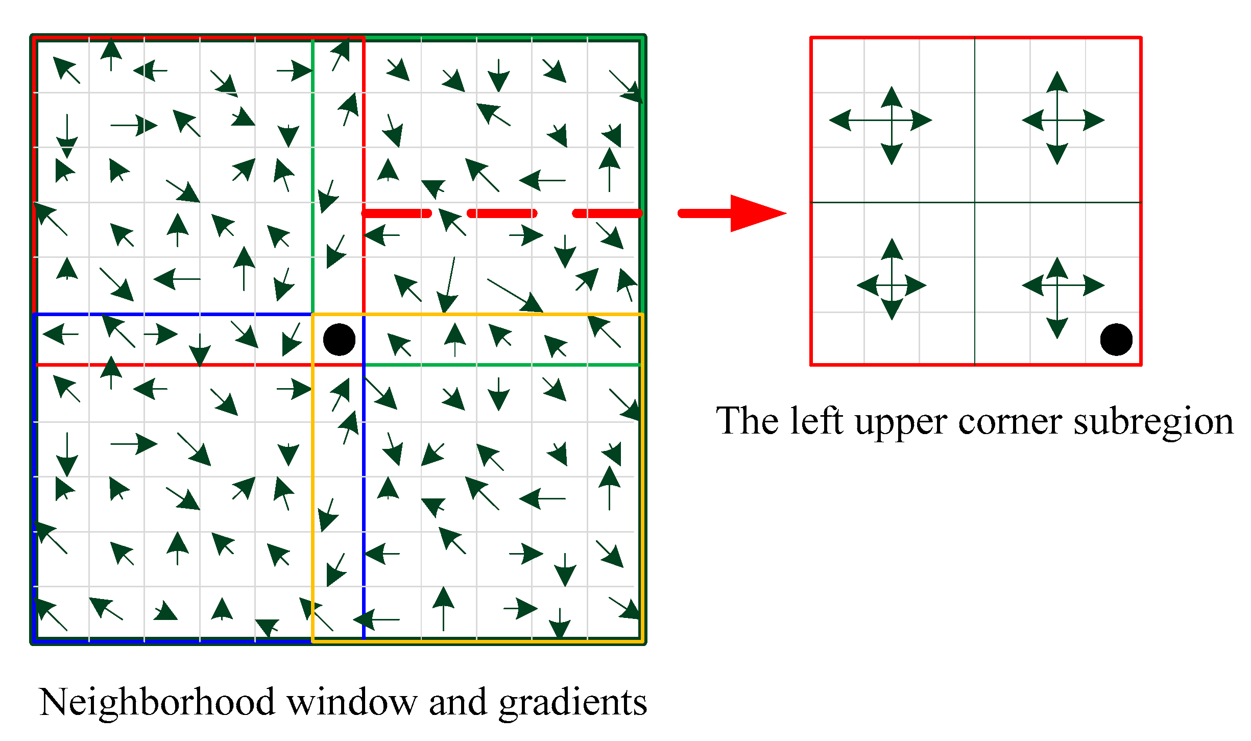
Firstly, Gaussian filtering is used to reduce the image noise. Then, the neighborhood window with a center at the target point is built for the descriptor construction. The size of the window is . In this study, we set . We assume that the coordinates of the target point are and the coordinates of the four corners of the neighborhood window are , , , and . The neighborhood window is then divided into four subregions, in which the square areas with the target point and the four corners of the neighborhood window are used to set the diagonals. The size of each subregion is . The schematic is shown in Figure 3. The four subregions with overlapping regions, which all include the row and column where the target point is located, are obtained. This strategy increases the correlation between regions and avoids the influence of region inconsistency caused by large viewpoint changes.
Secondly, each subregion is again divided into four square regions with the same sizes, and 16 small patches are obtained around the target point. A gradient magnitude histogram with four orientations is then calculated in each small patch. As the impact of the nearby points on the descriptor increases, the distance from each point in the patch to the target point is calculated, and each gradient magnitude is weighted by the corresponding distance with the function in the statistical process. Then, a statistical description vector about the gradient magnitudes in the four directions for each small patch is obtained, the description vectors of four small patches in the subregion are stacked, and a 4 × 4 description matrix for this subregion is obtained. Thereafter, inspired by the mean-standard deviation line descriptor (MSLD) descriptor [37], the mean and standard deviation vectors of matrix are calculated and normalized, respectively, to unit norm to make the descriptor invariant to linear changes of illumination. Finally, the descriptor vector with a length of 32 is obtained by concatenating the normalized mean vector of four subregions with the normalized standard deviation vector of four subregions into a single vector.
Our design of the descriptor adopts the subregions overlapping one another in the feature description, which increases the correlation between description vectors and contributes to the generation of dense matching results.
2.1.2. Dissimilarity Measure
For two points in any set of matching hypotheses in the first matching stage, the two descriptors and are obtained for the reference and search image points, and Euclidean distance is used to calculate the dissimilarities between the descriptors. If the Euclidean distance is smaller than the given threshold , then this set of matching hypotheses is considered correct, that is, the two points in the matching hypotheses are a pair of corresponding points.
2.2. Point Matching with Multiple Constraints
Points that could not be matched in the first stage are further matched using a strategy with multiple constraints as described below.
Firstly, for reference point with an initial candidate point denoted as , we define the searching region as a square with a center at point and a length of , where is a user-defined parameter. In this study, we set . All pixels in the searching window are regarded as matching candidates. For each candidate, we build its descriptor and calculate the Euclidean distance between two descriptors of reference and candidate point. If at least one candidate point satisfies the condition in which the value is smaller than the threshold , then the optimal matching with subpixel accuracy should be determined further by utilizing multiple constraints.
Secondly, we divide each candidate point satisfied by the Euclidean distance constraint mentioned above into grids and obtain a set of candidate subpixels. For each candidate subpixel, three dissimilarity measures are defined as described below.
The first dissimilarity measure is the distance of the candidate subpixel from the epipolar line corresponding to the reference point (Figure 4). In this study, the epipolar line is calculated using the fundamental matrix obtained by corresponding points [38]. Its formula is , where and are the corresponding points on both images, is the fundamental matrix, and and are the corresponding epipolar lines on both images. In theory, the corresponding points are located on the corresponding epipolar lines, but small deviations may exist due to the inaccuracy of the fundamental matrix.
The second dissimilarity measure is the distance of the candidate subpixel from the corresponding side in the corresponding triangle, as shown in Figure 4.
The third dissimilarity measure is related to the Mahalanobis distance, which was introduced by P.C. Mahalanobis in 1936. This distance is a measure of the distance between a point and a distribution. The formula is as follows:
where is a sample point, is the mean value of a set of sample points, and is the covariance matrix. In this study, the Mahalanobis distance can also be defined as a dissimilarity measure between two random vectors x and y of the same distribution with the covariance matrix ,
where and are two matched points in a single image. We suppose the corresponding points on both images are denoted by the two sets and . For any new point-to-point correspondence on both images, the Mahalanobis distance between and the corresponding points in the set is similar to that between and the corresponding points in the set . The dissimilarity measure is defined on the basis of this principle. To reduce the computational complexity, we only calculate the Mahalanobis distance between the point and the three vertices of the triangle where the point is located. We assume that and are the Mahalanobis distance vector of 3 × 1 corresponding to the reference and candidate points, respectively. We define the third dissimilarity measure as , where denotes the ratio of the sum of all elements in the vector and the total number of elements in the vector.
On the basis of the third dissimilarity measure mentioned above, we define two thresholds , where , and eliminate the candidate subpixels with any element in greater than or . Thus, only the subpixels fulfilling the two constraints above are retained. Then, an overall matching similarity score related to four dissimilarity measures is determined to achieve the optimal matching subpixel for the reference point.
where represents the different weights corresponding to four dissimilarity measures, in which . In this study, we set the weights to 0.45, 0.25, 0.15, and 0.15, respectively. As for all the remaining potential matching subpixels, we calculate and find the highest overall similarity score if the highest value is larger than the given threshold , which corresponds to the subpixel selected as the final matching point.
2.3. Matching Propagation
In the existing graph-based constraint matching, the images are divided into different regions by Delaunay triangulation or Voronoi, and many corresponding regions are usually obtained from two images. Matching propagation is performed within these regions (i.e., graph constraint matching propagation). On the basis of the principle in which the corresponding points are located within the corresponding regions, the matching search is conducted in the corresponding regions in different views. Most methods use the feature points extracted in the region as the matching primitives [16,26,28]. This propagation method belongs to the patch-to-patch propagation strategy or the triangle-to-triangle propagation strategy. Different from the region propagation strategies, a new edge-to-edge matching propagation strategy is adopted in this study. This new strategy uses the edge of the triangle as the carrier of matching propagation and the two types of points (midpoints and intersections) on the edge as the matching primitive. As the main principle of this propagation method, triangulation is updated by inserting newly matched points, new edges are generated as a means of obtaining new matching points, and matching is performed on the corresponding edges of the corresponding triangles in different views. Compared with the region-to-region propagation strategy, our proposed strategy offers the advantage of having an edge that is more stable than the region in theory. The principle of matching propagation is described in Algorithm 1.
| Algorithm 1 Matching propagation strategy to obtain quasi-dense matching |
| Input: Reference image and search image ; Initial reliable corresponding points Pt(Pt1,Pt2) ; Line segments Le extracted from the reference image; ; Output: Corresponding points |
| Return |
During matching propagation, we only deal with newly generating edges of triangles in the updating process of triangulation to avoid repeated matching in each iteration. The blue triangles shown in Figure 5a represent the initial triangulation, while the black and green points are the newly matched points (midpoints and intersections, respectively) generated by the first iteration. We insert the newly matched points into the initial triangulation and obtain the updated triangulation. The red edges of triangles in Figure 5b are the newly generated or split edges after the first matching, which are used in the subsequent iteration matching.
Figure 6 shows the results of the different stages of matching for the tested stereo pairs, with . Figure 6b presents the matching result of the second iterations, while Figure 6c shows the final matching result, that is, the result of the ninth iteration. Two types of matching primitives (the intersection points and midpoints) are matched by propagation, as shown by the green and red marks, respectively. The intersection points in Figure 7 are all located on the feature edge of the building, while the midpoints have an approximately uniform distribution. The numbers of the two types of points increase in each iteration (Figure 8). As the number of iterations increases, the number of corresponding points and triangles also increases, especially in the first four iterations in which the number of corresponding points increases greatly. The results of the intersection point and the midpoint are relatively stable after five and eight iterations, respectively. These phenomena are consistent with our original assumption that the number of midpoints increases accordingly with the increase in triangles in the iterations, whereas the number of extracted line segments in the image is fixed.
3. Further Experiments and Analysis
The performance of our method is evaluated by selecting twelve representative image pairs for the dense matching (Figure 9). These image pairs include various image transformations, such as viewpoint changes, scale changes, illumination, and rotation. A computer with a 3.6-GHz central processing unit (CPU) and 16 GB of random-access memory (RAM) is used for the experiment, and the code is implemented in Matlab 2016a. Extensive experiments are conducted to select the initial proper values for certain parameters of the proposed method. Then, hierarchical matching is performed in different scene images with determined parameters.
3.1. Parameter Selection
A method for accuracy assessment based on the homography matrix is adopted to assess the matching accuracy. Firstly, the homography matrix is calculated according to the corresponding points obtained by matching. Next, the corresponding points in the reference image are mapped onto the search image by using the homography matrix. The distance histogram is obtained according to the distance between the mapping and corresponding points. Finally, the inner and outer points are determined according to the distance histogram, and the matching accuracy is calculated.
The main parameters to be tuned in our method are , where , and . and are the descriptors for the dissimilarity measure threshold. is used to determine whether the correspondence hypothesis is correct in the first stage, and controls the matching hypotheses to be processed in the second matching stage. and are the parameters for the Mahalanobis distance constraint, and is the overall similarity score threshold used to determine the final matching points in the second stage. We firstly determine the approximate ranges of the parameters and steps according to the histogram distribution of the operation results of all image pairs. Then, initial parameter values are selected (Table 1) after the experimental analysis of representative image pairs. Thereafter, all the image pairs are used to for parametric analysis. Owing to the relatively complex interaction between the parameters in the iterative process and the parameter analysis of the unsupervised results, we adopt the following strategy to determine the parameters. We firstly set the initial parameter values and then update each of the parameters in turn according to the matching results. After parametric analysis of the first eight image pairs (Figure 9a–h) according to the above-mentioned strategy, we find that all test image pairs satisfy a set of parameter values optimally or have only small deviations from the initial parameter values; thus, this set of parameters is chosen as the final parameters for matching (Table 2).
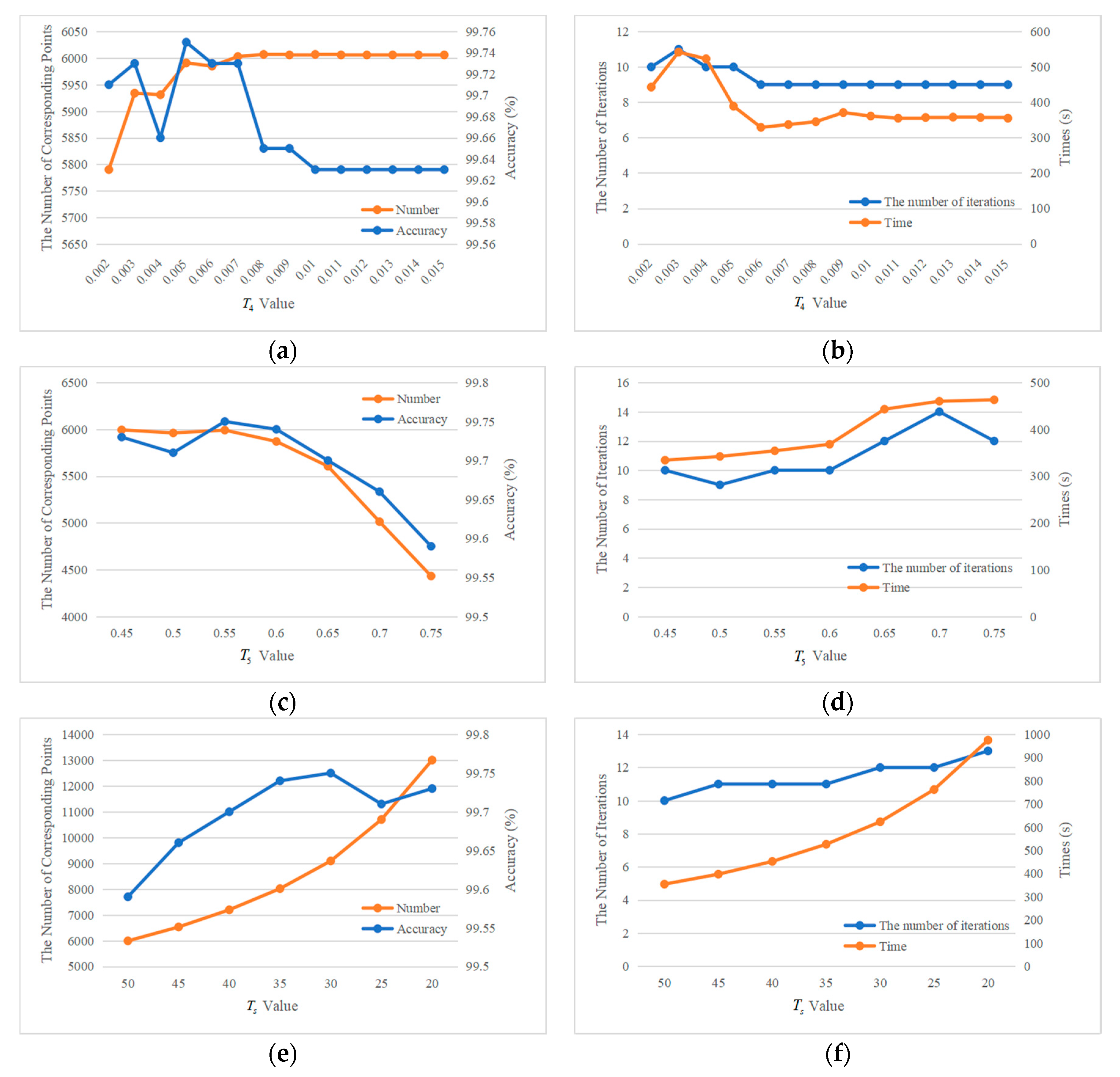
The image pair (a) in Figure 9, which is one of the image pairs corresponding to the optimal parameter, is taken as an example. We update parameters , where , and successively. The resulting curves with different parameter values are shown in Figure 10 and Figure 11. The graphs on the left show the number and accuracy of the matching, while the graphs on the right show the number of iterations and running time. The larger the two values on the left figures are and the smaller the two values in the right figures are, the better the matching result will be. As such, the optimal settings can be selected for the parameters or thresholds by combining the four factors mentioned above.
We firstly determine . The matching results with different values are shown in Figure 10a,b. The number and accuracy can reach their maximum values at the same time at , and the numbers of iterations are all 10. Clearly, the running time decreases with the increase in . This outcome is attributed to the number of matching hypotheses decreasing in the second matching stage during each iteration with the increase in , while the running time of the second stage is more time-consuming than the first stage. Thus, the running time is reduced.
We fix the value to and conduct the experiment with different values. The result is shown in Figure 10c,d. The accuracy yields the local peak at , and the number of iterations and run time reach the local minimum peak at the same time. The findings indicate that the initial value can be retained at .
Figure 10e,f show the results with different values. The number of matching result shows a rising trend with the increase in , and the accuracy yields a peak at . The time and the number of iterations are relatively stable even though the number of iterations is nine when is 0.007 or 0.008, and the corresponding accuracy is low. Therefore, must be selected in a manner wherein the above-mentioned aspects are balanced and is updated to 0.011.
Similar to , parameter constrains the matching candidates in the second stage. The larger both values are, the more candidate matches will be generated in each iteration. As shown in Figure 11a,b, the accuracy of the result can reach the local peak at , and the number, run time, and iteration times begin to gradually flatten from . This finding suggests that the initial value can be retained.
For matching candidates obtained by the above-mentioned and constraints, we calculate the overall similarity score for each candidate and determine the highest score. If the highest score is larger than , then the candidate corresponding to the highest score will be selected as the final corresponding point. As shown in Figure 11c,d, the number of matching presents a downtrend with the increase in , and the accuracy yields a peak at . This result indicates that the initial value can be retained.
is the area of the triangle threshold that controls the size of the propagation triangle. The smaller is, the denser the matching results will be in general. This scenario can also be observed in Figure 11e,f, in which the number of corresponding points increases with the decrease in , and the running time is significantly increased at the same time. Although the number of matched points can reach the local maximum at , , which has the highest accuracy, is eventually selected in this study when running time is considered.
Notably, our method has low sensitivity toward different parameters within a certain range, in which the numbers and accuracies of matching points only have slight differences, and the matching results are relatively stable. Given that the proposed method is an iteration matching method, the last matching result will directly affect the matching result of the next iteration, and the effect of the different parameters on the result is relatively complex. Therefore, some signs can still be followed despite the difficulty in achieving consistent regularity for the whole scheme.
3.2. Different Matching Stages
Table 2 presents the required parameters that are finally determined according to the parametric analysis in Section 3.1. The proposed method is used for the dense matching of the 12 sets of images previously shown in Figure 9. The experimental results are listed in Table 3 and depicted in Figure 12. The columns in Table 3 represent the number of initial corresponding points, the stage of finished matching, the number of matching iterations, the number of matched midpoints, the number of matched intersection points, the number of all corresponding points, the number of incorrect matching, the matching accuracy, and the running time, respectively.
The results in Table 3 show several findings. Firstly, the proposed method utilizes the two-stage hierarchical matching strategy. The number of corresponding points can be increased by adding an implementation of the second matching stage, which will improve the accuracy of some results. However, with the increase in the number of corresponding points and the computational complexity in the second matching stage, the method will be a time-consuming process. Secondly, the number of matched midpoints is higher than the number of matched intersections for the two matching primitives. This phenomenon can be explained by the number of midpoints, which increases dynamically in the iterative matching process. By contrast, the number of extracted line segments is fixed, while that of the matched intersections tends to be stable after a few iterations. Thirdly, as shown by the corresponding points and their distribution in different colors in Figure 11, the corresponding points manifest a consistent distribution. Lastly, as for the experimental images selected in this study, the matching accuracies of the method all exceed 98%, which indicates the method’s high accuracy. This result can be attributed to the strict constraints of the algorithm and the reliability of the descriptors. The robustness of the method is also verified by the different types of image matching experiments.
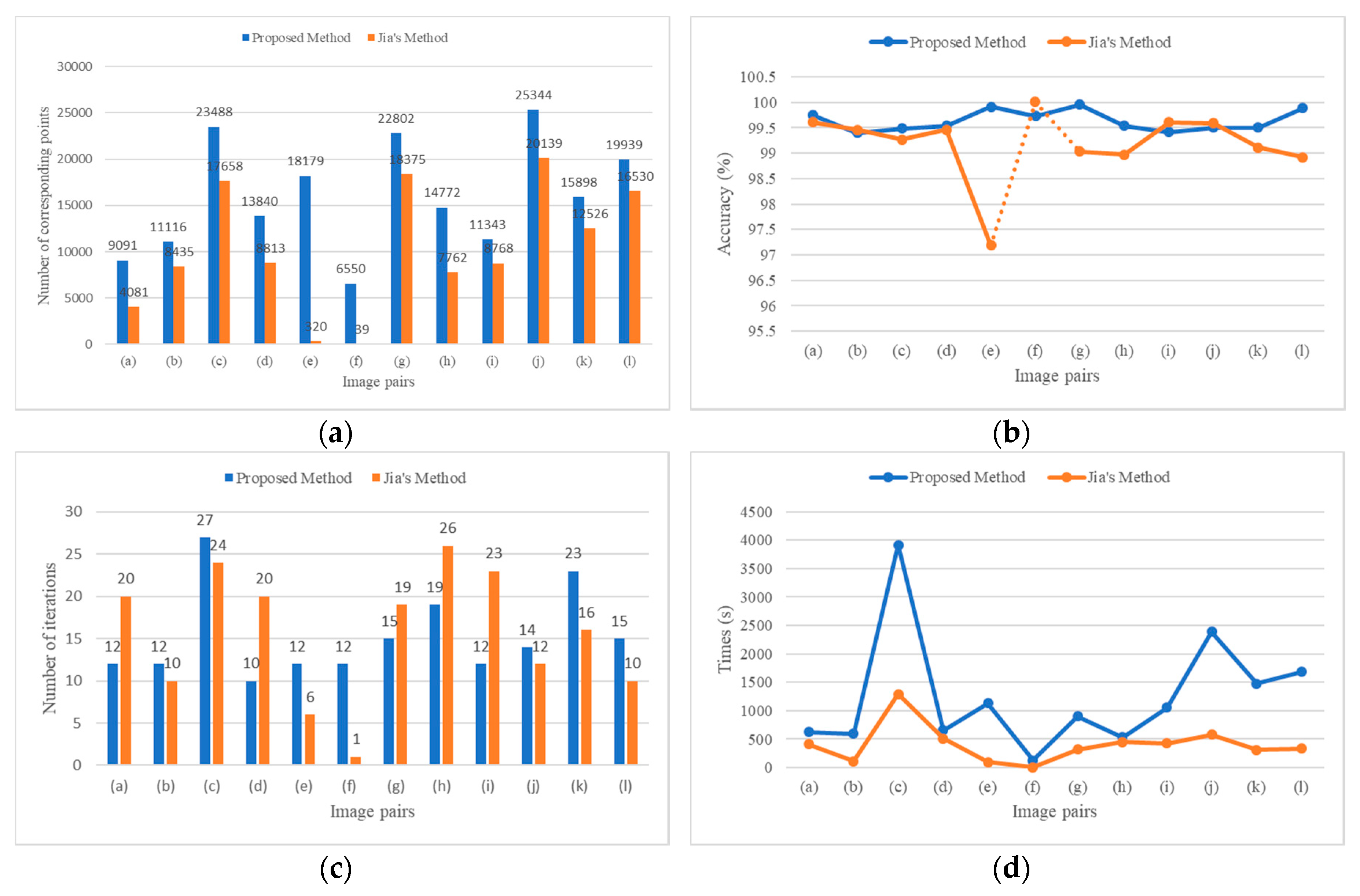
3.3. Comparison with Jia’s Method
We compare the results of the proposed method with the results of the quasi-dense matching method presented in Jia (2019). In order to perform a comparative analysis of the two methods under consistent conditions, we utilize the same initial corresponding points to construct initial triangulations during the implementation of Jia’s method. Similar to our method, only triangles with an area greater than 30 are used for matching propagation in the matching process. The comparison results of the number of corresponding points, accuracy, the number of iterations, and running times of the two methods for 12 sets of image pairs are provided in Figure 13. As observed, the number of corresponding points of the proposed method is greater than that of Jia’s method for all test images, where Jia’s method fails in image pairs (e) and (f). In terms of accuracy, the accuracy of both methods is above 97%. However, the accuracy of the proposed method is higher than that of Jia’s method for most of the image pairs. Notably, Jia’s method has an accuracy of 100% at image pair (f), but this accuracy belongs to the accuracy of the initial seed point because Jia’s method fails in image pair (f) and does not obtain the corresponding point. However, no regularity is observed in the number of iterations between the two methods due to the complexity of the iterative process. We also compare the computation times required by the two methods. The results show that our method runs 0.1–4.1 times slower than Jia’s method, except for the image pairs (e) and (f). These results are due to three reasons. Firstly, the proposed method is designed using two matching stages; points that do not meet the descriptor similarity constraint in the first stage are further matched by extending the matching candidates and using multiple constraints, which increases the number of matches while ensuring match reliability. Secondly, compared with similarity constraints of single-pixel color information in Jia’s method, our constructed gradient descriptors are more robust for different images, especially for images with illumination change. The proposed method produces higher dense matching results, whereas Jia’s method fails to match. Thirdly, although the above-mentioned aspects contribute to the dense matching results of the proposed method, they require heavy workload. As a result, Jia’s method achieves better computation times than our method, but the proposed method outperforms Jia’s method in terms of robustness and density.
4. Conclusions
A hierarchical method based on triangulation constraint and propagation for the dense matching of points from a close-range image is proposed. The matching begins from the initial triangulation constructed by the initial corresponding points generated using the SIFT method. The correspondences between the image pairs are established with the midpoints and intersection points in the edges of the triangles as matching primitives. The characteristics of the proposed method are manifold. Firstly, we utilize points in the edges of triangles as the matching primitives and then conduct edge-to-edge matching propagation in the process of matching iteration. Our approach is more stable in theory than the region-to-region propagation. Secondly, we use two types of matching strategies for the different matching stages. We further match points that cannot be matched by the descriptor similarity in the first stage by utilizing multiple constraints. An overall matching similarity score is defined for the multiple constraints with different weights. In this manner, the number of matching results can be increased, and the reliability of the matching can be enhanced. Thirdly, two aspects need to be considered in improving the efficiency of the matching. The first aspect focuses on the multithreading technique for improving processing performance. The second aspect is only for the newly generated triangle edges, which are processed in each iteration matching to avoid repeated matching. Fourthly, the descriptor construction with overlapping subregions can improve the reliability of the descriptors and effectively restrain the propagation of mismatches. Lastly, intersections between feature line segments and triangle edges are introduced as the matching primitive. This way enriches the edge information of the result.
The results of the 12 typical close-range image pairs show that matching accuracy can exceed 98%. Thus, the proposed method has high robustness for different images and can obtain reliable matching results. In the future, we plan to change the range of matching results in images, from the coverage of corresponding points to the maximum overlap of image pairs, by performing an outward growth of a region with seed points. We plan to conduct tests to validate if the method can also obtain reliable results for aerial images. We also intend to transform the matching results into discrete point clouds for further 3D reconstruction.
Author Contributions
Writing—review and editing, Jingxue Wang; Methodology, Writing—original draft, Ning Zhang; Resources, Xiangqian Wu; Funding acquisition, Jingxue Wang and Weixi Wang. All authors have read and agreed to the published version of the manuscript.
Funding
This research was funded by National Natural Science Foundation of China grant number 41871379 and 41971354.
Acknowledgments
We would like to thank all the anonymous reviewers for their valuable comments, which helped us to improve this manuscript.
Conflicts of Interest
The authors declare no conflict of interest.
References
- Wang, D.; Liu, H.; Cheng, X. A miniature binocular endoscope with local feature matching and stereo matching for 3d measurement and 3d reconstruction. Sensors 2018, 18, 2243. [Google Scholar] [CrossRef] [PubMed] [Green Version]
- Yang, W.; Li, X.; Yang, B.; Fu, Y. A novel stereo matching algorithm for digital surface model (DSM) generation in water areas. Remote Sens. 2020, 12, 870. [Google Scholar] [CrossRef] [Green Version]
- Su, N.; Yan, Y.; Qiu, M.; Zhao, C.; Wang, L. Object-based dense matching method for maintaining structure characteristics of linear buildings. Sensors 2018, 18, 1035. [Google Scholar] [CrossRef] [PubMed] [Green Version]
- Lhuillier, M.; Quan, L. Match propagation for image-based modeling and rendering. IEEE Trans. Pattern Anal. Mach. Intell. 2002, 24, 1140–1146. [Google Scholar] [CrossRef]
- Tola, E.; Lepetit, V.; Fua, P. A fast local descriptor for dense matching. In Proceedings of the 2008 26th IEEE Conference on Computer Vision and Pattern Recognition, Anchorage, AK, USA, 23–28 June 2008; pp. 1–15. [Google Scholar] [CrossRef] [Green Version]
- Gruen, A. Development and Status of Image Matching in Photogrammetry. Photogramm. Rec. 2012, 27, 36–57. [Google Scholar] [CrossRef]
- Yu, Z.; Guo, X.; Ling, H.; Lumsdaine, A.; Yu, J. Line assisted light field triangulation and stereo matching. In Proceedings of the IEEE International Conference on Computer Vision, Sydney, Australia, 1–8 December 2013; pp. 2792–2799. [Google Scholar] [CrossRef] [Green Version]
- Revaud, J.; Weinzaepfel, P.; Harchaoui, Z.; Schmid, C. DeepMatching: Hierarchical Deformable Dense Matching. Int. J. Comput. Vis. 2016, 120, 300–323. [Google Scholar] [CrossRef] [Green Version]
- Dong, X.; Shen, J.; Shao, L. Hierarchical Superpixel-to-Pixel Dense Matching. IEEE Trans. Circuits Syst. Video Technol. 2017, 27, 2518–2526. [Google Scholar] [CrossRef] [Green Version]
- Jia, D.; Zhao, M.; Cao, J. FDM: Fast dense matching based on sparse matching. Signal Image Video Process. 2020, 14, 295–303. [Google Scholar] [CrossRef]
- Zhang, K.; Sheng, Y.; Ye, C. Stereo image matching for vehicle-borne mobile mapping system based on digital parallax model. Int. J. Veh. Technol. 2011, 2011, 1–11. [Google Scholar] [CrossRef] [Green Version]
- Laraqui, M.; Saaidi, A.; Mouhib, A.; Abarkan, M. Images Matching Using Voronoï Regions Propagation. 3D Res. 2015, 6, 1–16. [Google Scholar] [CrossRef]
- Khazaei, H.; Mohades, A. Fingerprint matching algorithm based on voronoi diagram. In Proceedings of the 2008 International Conference on Computational Sciences and Its Applications, Perugia, Italy, 30 June–3 July 2008; pp. 433–440. [Google Scholar] [CrossRef]
- Wu, J.; Wan, Y.; Chiang, Y.Y.; Fu, Z.; Deng, M. A Matching Algorithm Based on Voronoi Diagram for Multi-Scale Polygonal Residential Areas. IEEE Access 2018, 6, 4904–4915. [Google Scholar] [CrossRef]
- Soleymani, R.; Chehel Amirani, M. A hybrid fingerprint matching algorithm using Delaunay triangulation and Voronoi diagram. In Proceedings of the 20th Iranian Conference on Electrical Engineering (ICEE2012), Tehran, Iran, 15–17 May 2012; pp. 752–757. [Google Scholar] [CrossRef]
- Jiang, S.; Jiang, W. Reliable image matching via photometric and geometric constraints structured by Delaunay triangulation. ISPRS J. Photogramm. Remote Sens. 2019, 153, 1–20. [Google Scholar] [CrossRef]
- Zhu, Q.; Wu, B.; Tian, Y. Propagation strategies for stereo image matching based on the dynamic triangle constraint. ISPRS J. Photogramm. Remote Sens. 2007, 62, 295–308. [Google Scholar] [CrossRef]
- Li, T.; Sui, H.T.; Wu, C.K. Dense Stereo Matching Based on Propagation with a Voronoi Diagram. In Proceedings of the Third Indian Conference on Computer Vision, Graphics & Image Processing, Ahmadabad, India, 16–18 December 2002. [Google Scholar]
- Finch, A.M.; Wilson, R.C.; Hancock, E.R. Matching delaunay triangulations by probabilistic relaxation. In International Conference on Computer Analysis of Images and Patterns; Springer: Berlin/Heidelberg, Germany, 1995; Volume 970, pp. 350–358. [Google Scholar] [CrossRef]
- Lhuillier, M.; Quan, L. Image interpolation by joint view triangulation. In Proceedings of the 1999 IEEE Computer Society Conference on Computer Vision and Pattern Recognition, Fort Collins, CO, USA, 23–25 June 1999; Volume 2, pp. 139–145. [Google Scholar] [CrossRef] [Green Version]
- Sedaghat, A.; Ebadi, H.; Mokhtarzade, M. Image Matching of Satellite Data Based on Quadrilateral Control Networks. Photogramm. Rec. 2012, 27, 423–442. [Google Scholar] [CrossRef]
- Liu, Z.; An, J.; Jing, Y. A simple and robust feature point matching algorithm based on restricted spatial order constraints for aerial image registration. IEEE Trans. Geosci. Remote Sens. 2012, 50, 514–527. [Google Scholar] [CrossRef]
- Zhao, M.; An, B.; Wu, Y.; Chen, B.; Sun, S. A Robust delaunay triangulation matching for multispectral/multidate remote sensing image registration. IEEE Geosci. Remote Sens. Lett. 2015, 12, 711–715. [Google Scholar] [CrossRef]
- Ma, J.; Ahuja, N. Region Correspondence by Global Con guration Matching and Progressive Delaunay Triangulation. In Proceedings of the IEEE Conference on Computer Vision and Pattern Recognition, Hilton Head Island, SC, USA, 13–15 June 2000; Volume 2, pp. 637–642. [Google Scholar] [CrossRef]
- Guo, X.; Cao, X. Good match exploration using triangle constraint. Pattern Recognit. Lett. 2012, 33, 872–881. [Google Scholar] [CrossRef]
- Zhu, Q.; Zhao, J.; Lin, H.; Gong, J. Triangulation of well-defined points as a constraint for reliable image matching. Photogramm. Eng. Remote Sens. 2005, 71, 1063–1069. [Google Scholar] [CrossRef]
- Zhu, Q.; Zhang, Y.; Wu, B.; Zhang, Y. Multiple close-range image matching based on a self-adaptive triangle constraint. Photogramm. Rec. 2010, 25, 437–453. [Google Scholar] [CrossRef]
- Wu, B.; Zhang, Y.; Zhu, Q. Integrated point and edge matching on poor textural images constrained by self-adaptive triangulations. ISPRS J. Photogramm. Remote Sens. 2012, 68, 40–55. [Google Scholar] [CrossRef]
- Jia, D.; Wu, S.; Zhao, M. Dense matching for wide baseline images based on equal proportion of triangulation. Electron. Lett. 2019, 55, 380–382. [Google Scholar] [CrossRef]
- Low, D.G. Distinctive image features from scale-invariant keypoints. Int. J. Comput. Vis. 2004, 60, 91–110. [Google Scholar] [CrossRef]
- Fischler, M.A.; Bolles, R.C. Paradigm for Model. Commun. ACM 1981, 24, 381–395. [Google Scholar] [CrossRef]
- Lowe, D.G. Object recognition from local scale-invariant features. In Proceedings of the Seventh IEEE International Conference on Computer Vision, Kerkyra, Greece, 20–27 September 1999; Volume 2, pp. 1150–1157. [Google Scholar] [CrossRef]
- Sun, Y.; Zhao, L.; Huang, S.; Yan, L.; Dissanayake, G. L2-SIFT: SIFT feature extraction and matching for large images in large-scale aerial photogrammetry. ISPRS J. Photogramm. Remote Sens. 2014, 91, 1–16. [Google Scholar] [CrossRef]
- Wang, E.; Jiao, J.; Yang, J.; Liang, D.; Tian, J. Tri-SIFT: A triangulation-based detection and matching algorithm for fish-eye images. Information 2018, 9, 299. [Google Scholar] [CrossRef] [Green Version]
- Morel, J.M.; Yu, G. ASIFT: A new framework for fully affine invariant image comparison. SIAM J. Imaging Sci. 2009, 2, 438–469. [Google Scholar] [CrossRef]
- Tola, E.; Lepetit, V.; Fua, P. DAISY: An efficient dense descriptor applied to wide-baseline stereo. IEEE Trans. Pattern Anal. Mach. Intell. 2010, 32, 815–830. [Google Scholar] [CrossRef] [PubMed] [Green Version]
- Wang, Z.; Wu, F.; Hu, Z. MSLD: A robust descriptor for line matching. Pattern Recognit. 2009, 42, 941–953. [Google Scholar] [CrossRef]
- Moisan, L.; Stival, B. A Probabilistic Criterion to Detect Rigid Point Matches Between Two. Int. J. Comput. Vis. 2004, 57, 201–218. [Google Scholar] [CrossRef]
Figure 1.
Flowchart of the proposed method.

Figure 2.
Two types of matching primitives and their corresponding matching hypotheses. Three sets of midpoint correspondence hypotheses are , , and ; is an intersection point correspondence hypothesis.
Figure 2.
Two types of matching primitives and their corresponding matching hypotheses. Three sets of midpoint correspondence hypotheses are , , and ; is an intersection point correspondence hypothesis.
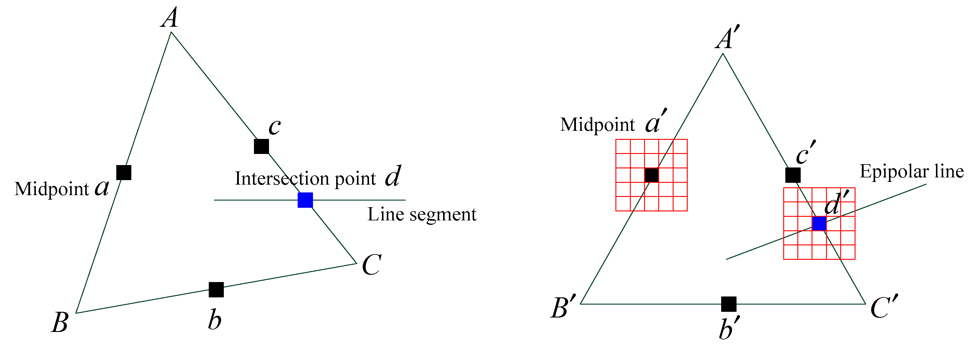
Figure 3.
Schematic of the point descriptor construction.

Figure 4.
Multiple constraints.
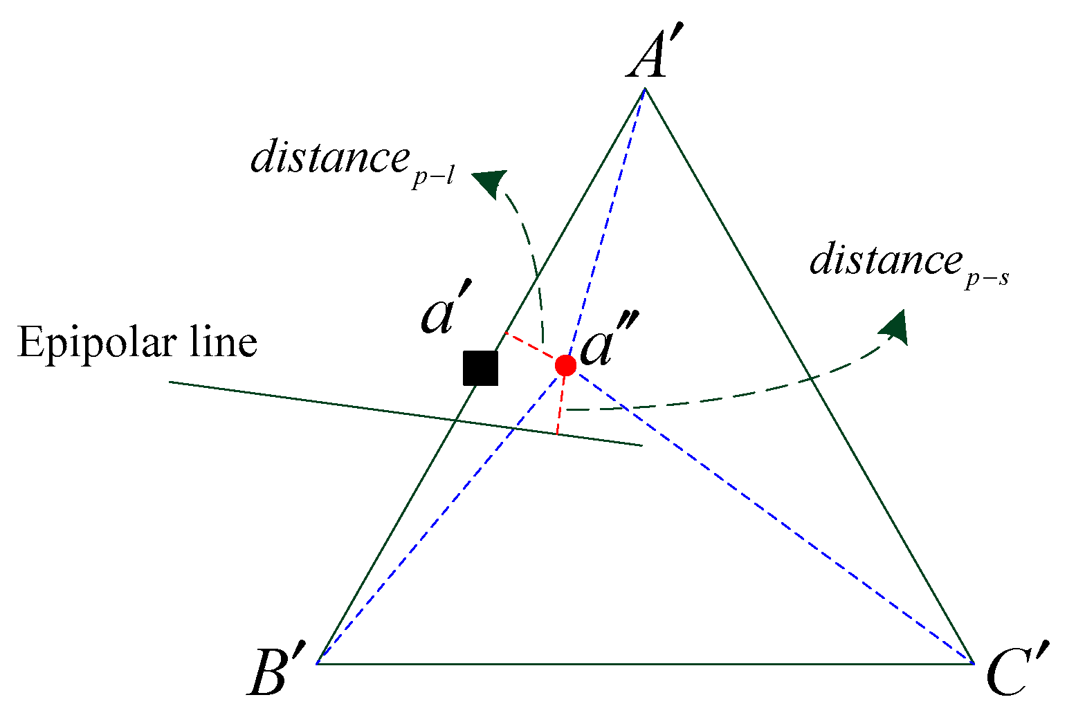
Figure 5.
Propagating process of matching: (a) initial triangulation and two types of newly matched points; (b) updated triangulation using newly matched points.
Figure 5.
Propagating process of matching: (a) initial triangulation and two types of newly matched points; (b) updated triangulation using newly matched points.
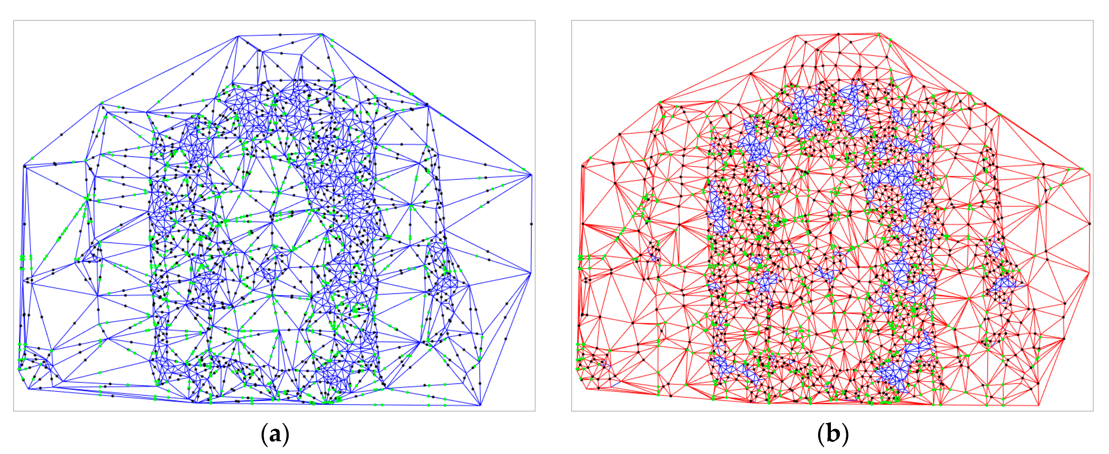
Figure 6.
Propagating process of matching: (a) initial matching result; (b) further matching result; (c) final matching result.
Figure 6.
Propagating process of matching: (a) initial matching result; (b) further matching result; (c) final matching result.

Figure 7.
Zoomed view of the final triangulation from the two types of matching primitives.
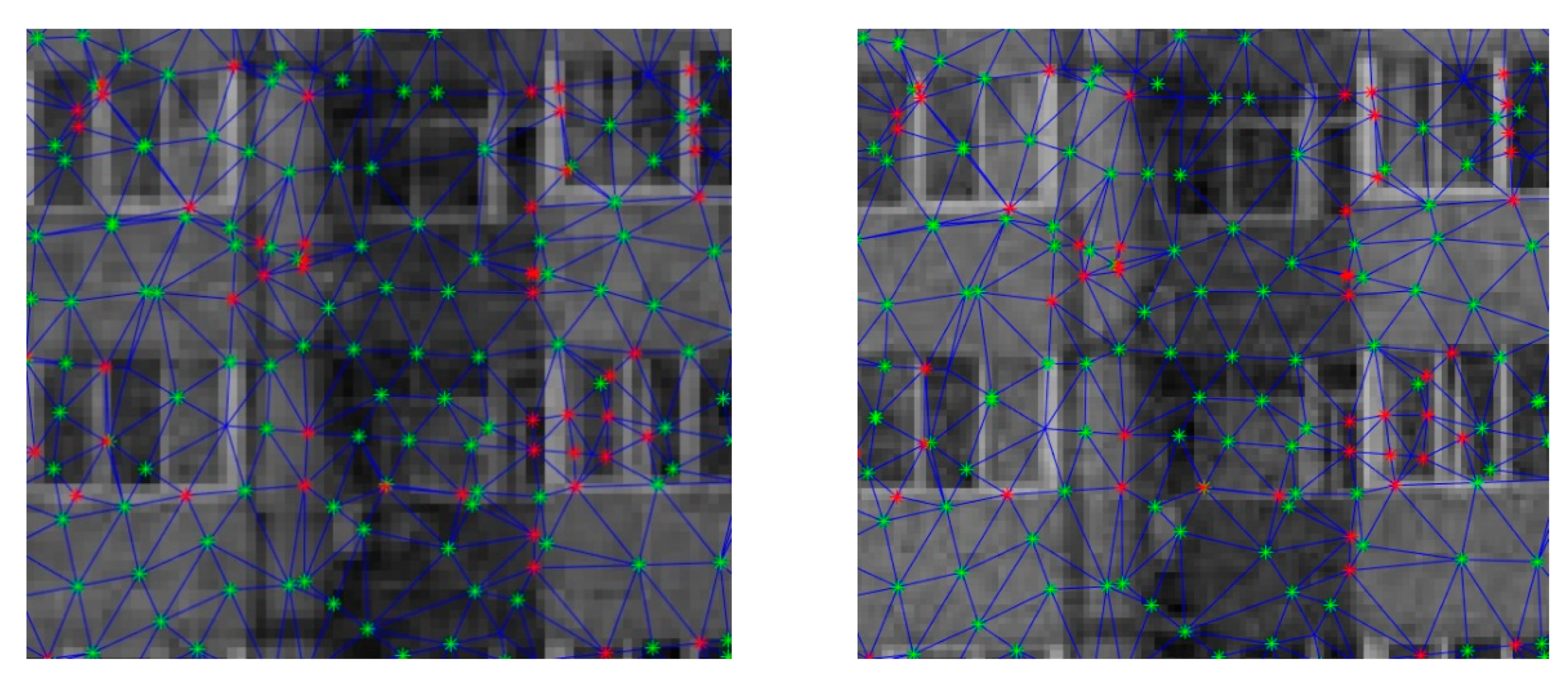
Figure 8.
Numbers of different types of corresponding points and triangles in varying stages of matching iterations.
Figure 8.
Numbers of different types of corresponding points and triangles in varying stages of matching iterations.

Figure 9.
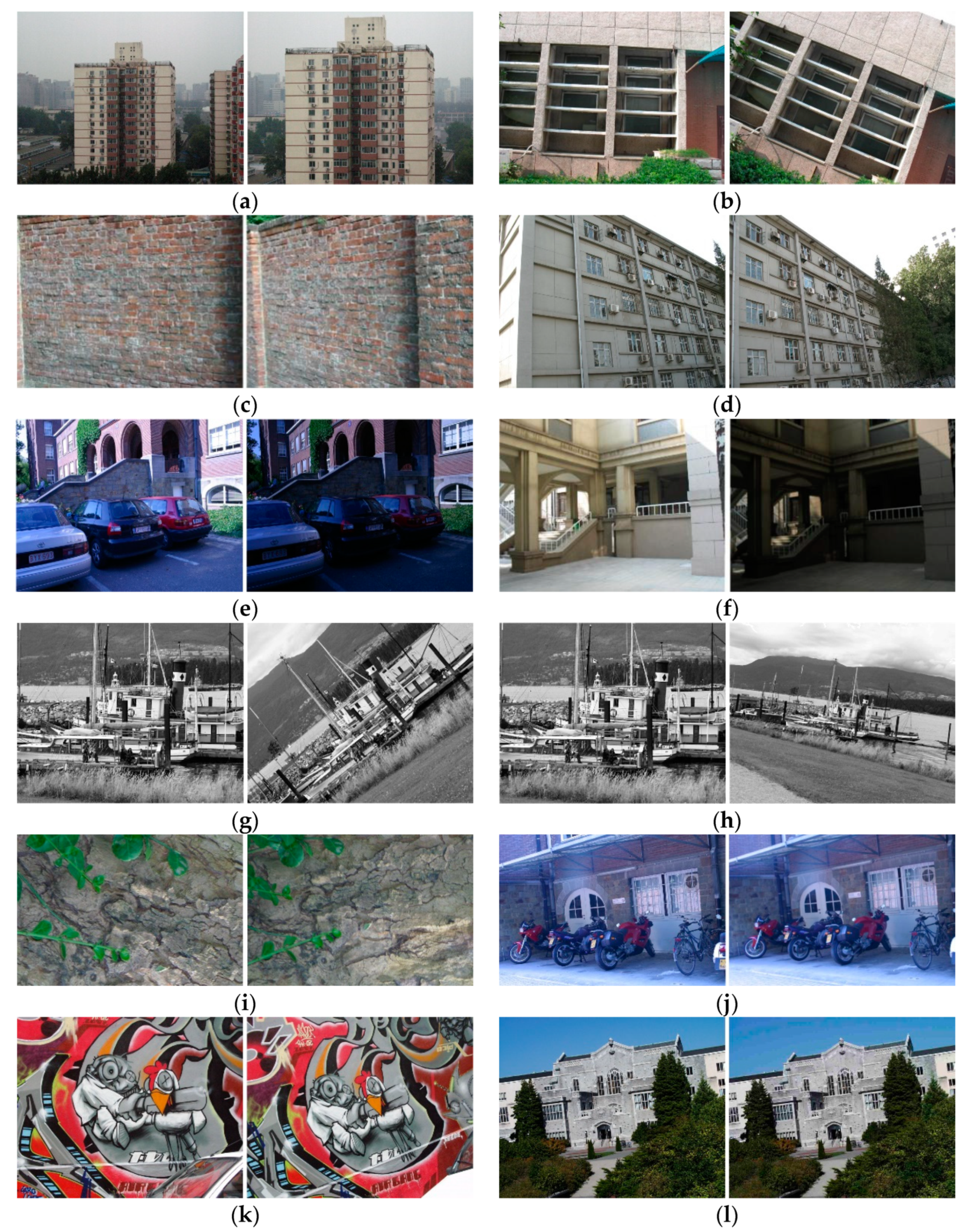
Image dataset. (a)Scale, (b) Rotation, (c) Viewpoint, (d) Viewpoint, (e) Illumination, (f) Illumination, (g) Rotation, (h) Rotation + Scale, (i) Rotation, (j) Blur, (k) Viewpoint, (l) JPEG compression.
Figure 9.
Image dataset. (a)Scale, (b) Rotation, (c) Viewpoint, (d) Viewpoint, (e) Illumination, (f) Illumination, (g) Rotation, (h) Rotation + Scale, (i) Rotation, (j) Blur, (k) Viewpoint, (l) JPEG compression.

Figure 10.
Matching results of different parameters: (a,c,e) represent the number of corresponding points and accuracy of matching; (b,d,f) represent the number of matching iterations and running time of the proposed method.
Figure 10.
Matching results of different parameters: (a,c,e) represent the number of corresponding points and accuracy of matching; (b,d,f) represent the number of matching iterations and running time of the proposed method.
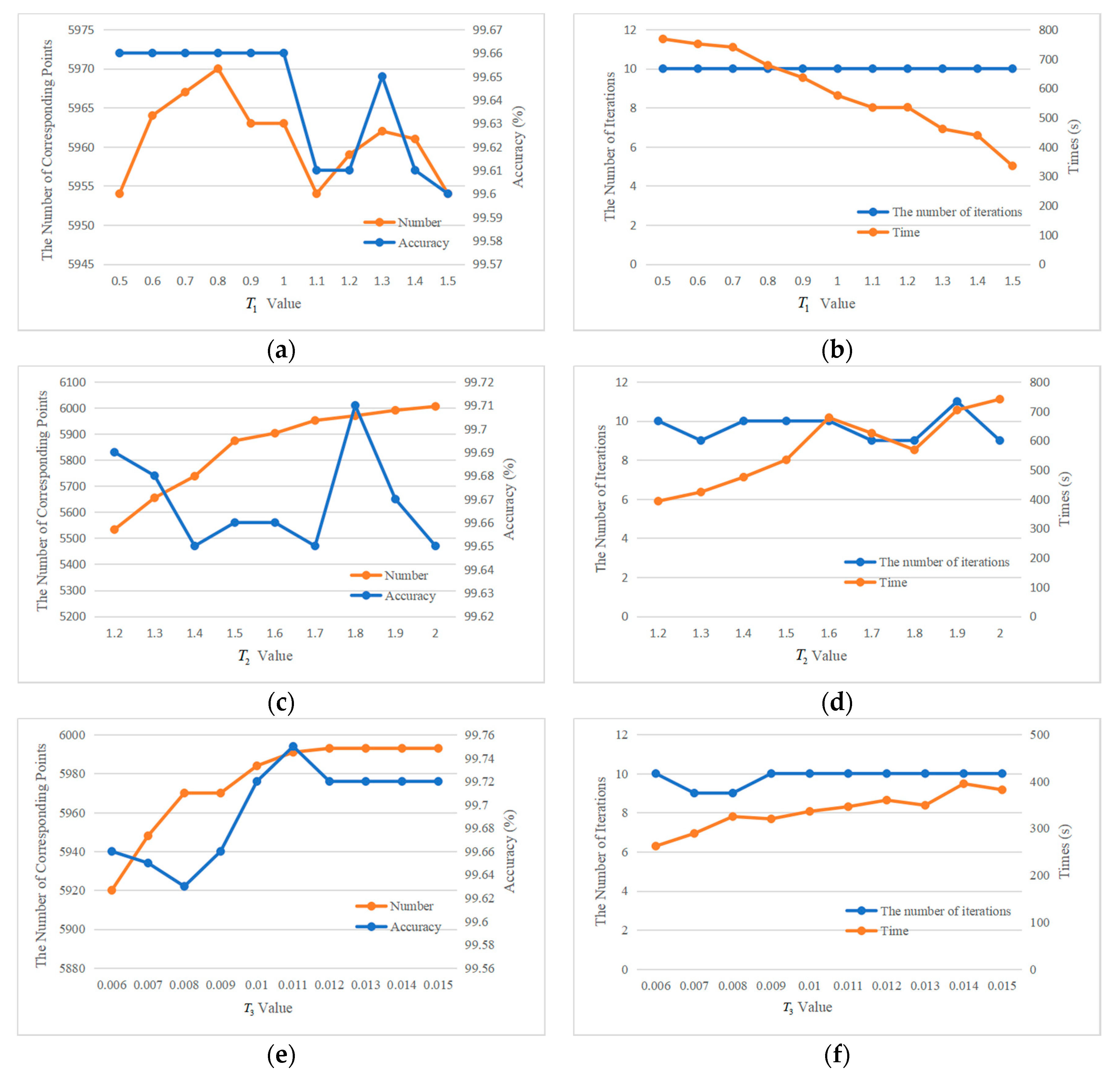
Figure 11.
Matching results of different parameters: (a,c,e) represent the number of corresponding points and accuracy of matching; (b,d,f) represent the number of matching iterations and running time of the proposed method.
Figure 11.
Matching results of different parameters: (a,c,e) represent the number of corresponding points and accuracy of matching; (b,d,f) represent the number of matching iterations and running time of the proposed method.

Figure 12.
Matching result of the proposed method for image pairs, with corresponding points shown in green and blue color gradients. (a,c,e,g,i,k,m,o,q,s,u,w) are the reference image in each image pair, respectively; (b,d,f,h,j,l,n,p,r,t,v,x) are the search image in each image pair, respectively.
Figure 12.
Matching result of the proposed method for image pairs, with corresponding points shown in green and blue color gradients. (a,c,e,g,i,k,m,o,q,s,u,w) are the reference image in each image pair, respectively; (b,d,f,h,j,l,n,p,r,t,v,x) are the search image in each image pair, respectively.
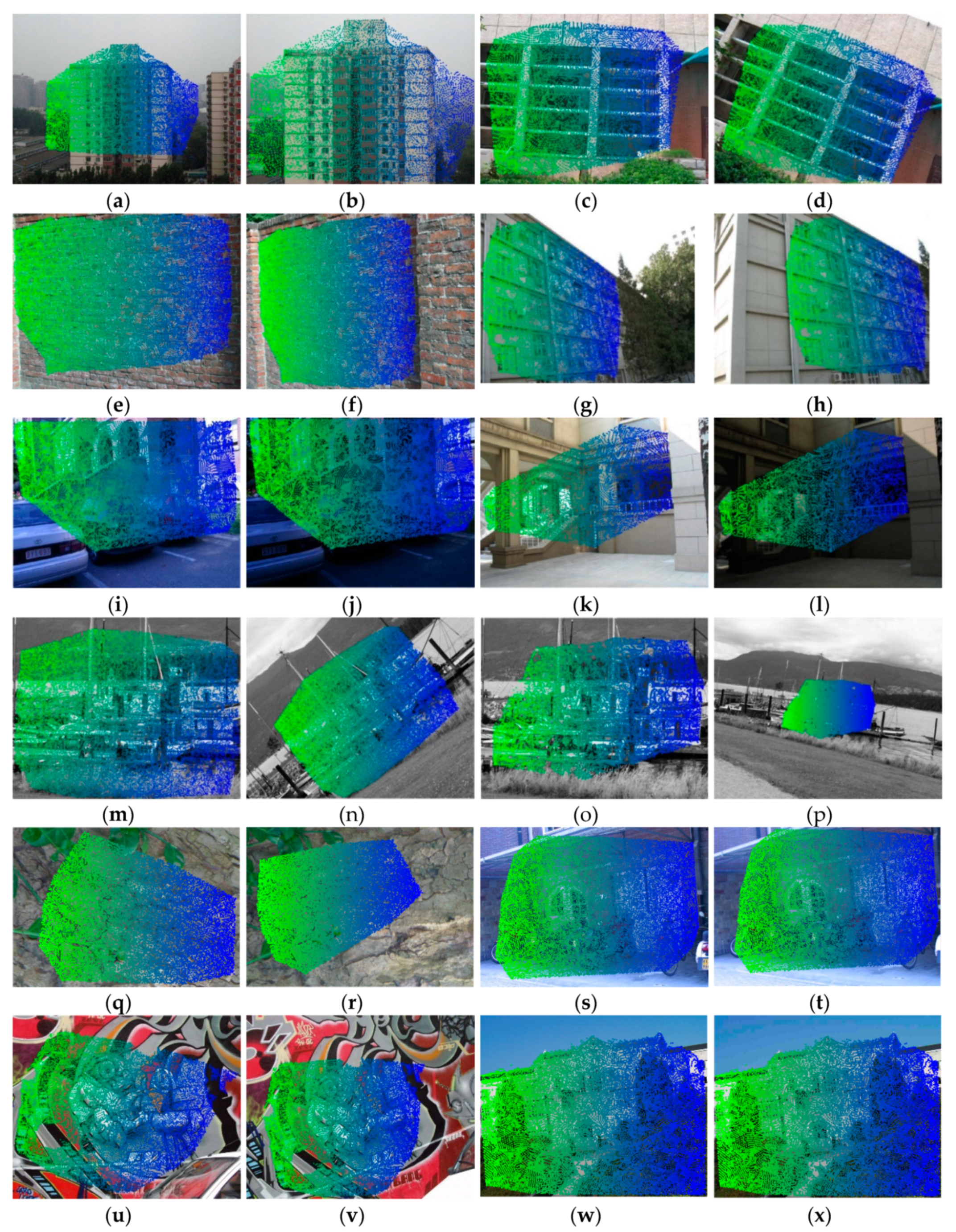
Figure 13.
Comparison of the proposed method and Jia’s method for 12 sets of image pairs: (a) number of matched points obtained by both methods; (b) accuracy of the two methods; (c) number of iterations of the two methods; (d) running times of the two methods.
Figure 13.
Comparison of the proposed method and Jia’s method for 12 sets of image pairs: (a) number of matched points obtained by both methods; (b) accuracy of the two methods; (c) number of iterations of the two methods; (d) running times of the two methods.

Table 1.
Initial threshold values for matching.
| Parameters | ||||||
|---|---|---|---|---|---|---|
| Value | 1.8 | 0.009 | 0.005 | 0.55 | 50 | |
| Range | 0.5–1.5 | 1.2–2 | 0.006–0.015 | 0.002–0.015 | 0.45–0.75 | 50–20 |
| Step | 0.1 | 0.1 | 0.001 | 0.001 | 0.05 | −5 |
Table 2.
Final selected thresholds and parameters for matching.
| Parameters | ||||||||||
|---|---|---|---|---|---|---|---|---|---|---|
| Value | 0.8 | 1.8 | 0.011 | 0.005 | 0.55 | 30 | 0.45 | 0.25 | 0.15 | 0.15 |
Table 3.
Comparison of matching results of the proposed method in different stages for twelve image pairs.
Table 3.
Comparison of matching results of the proposed method in different stages for twelve image pairs.
| Images | Seed Points | Stage | Number of Iterations | Number of Midpoints | Number of Intersections | Total | Wrong | Accuracy (%) | Time (s) |
|---|---|---|---|---|---|---|---|---|---|
| (a) | 911 | 1 | 13 | 2760 | 1767 | 5436 | 23 | 99.58 | 83 |
| 2 | 12 | 6016 | 2185 | 9091 | 23 | 99.75 | 623 | ||
| (b) | 213 | 1 | 14 | 4749 | 2674 | 7634 | 24 | 99.69 | 64 |
| 2 | 12 | 8014 | 2905 | 11,116 | 67 | 99.4 | 591 | ||
| (c) | 635 | 1 | 24 | 10,592 | 2863 | 14,088 | 60 | 99.57 | 852 |
| 2 | 27 | 19,069 | 3826 | 23,488 | 119 | 99.49 | 3916 | ||
| (d) | 463 | 1 | 13 | 6794 | 4613 | 11,868 | 56 | 99.53 | 211 |
| 2 | 10 | 8530 | 4865 | 13,840 | 63 | 99.54 | 655 | ||
| (e) | 302 | 1 | 18 | 10,028 | 3952 | 14,280 | 40 | 99.72 | 336 |
| 2 | 12 | 13,838 | 4060 | 18,179 | 17 | 99.91 | 1134 | ||
| (f) | 39 | 1 | 21 | 3415 | 1855 | 5307 | 24 | 99.55 | 27 |
| 2 | 12 | 4581 | 1937 | 6550 | 18 | 99.73 | 125 | ||
| (g) | 750 | 1 | 37 | 2351 | 2119 | 5218 | 58 | 98.89 | 117 |
| 2 | 15 | 16,468 | 5690 | 22,802 | 8 | 99.96 | 904 | ||
| (h) | 190 | 1 | 14 | 2988 | 1920 | 5096 | 46 | 99.09 | 80 |
| 2 | 19 | 10,139 | 4516 | 14,772 | 67 | 99.54 | 536 | ||
| (i) | 89 | 1 | 18 | 1047 | 1226 | 2360 | 15 | 99.36 | 108 |
| 2 | 12 | 9090 | 2195 | 11,343 | 66 | 99.42 | 1058 | ||
| (j) | 192 | 1 | 21 | 12,994 | 5620 | 18,804 | 133 | 99.29 | 1232 |
| 2 | 14 | 19,509 | 5684 | 25,344 | 127 | 99.50 | 2392 | ||
| (k) | 233 | 1 | 14 | 6265 | 3729 | 10,225 | 53 | 99.48 | 404 |
| 2 | 23 | 11,533 | 4162 | 15,898 | 81 | 99.50 | 1479 | ||
| (l) | 724 | 1 | 18 | 10,958 | 3667 | 15,347 | 42 | 99.79 | 649 |
| 2 | 15 | 15,591 | 3640 | 19,939 | 23 | 99.89 | 1683 |
© 2020 by the authors. Licensee MDPI, Basel, Switzerland. This article is an open access article distributed under the terms and conditions of the Creative Commons Attribution (CC BY) license (http://creativecommons.org/licenses/by/4.0/).
Share and Cite
MDPI and ACS Style
Wang, J.; Zhang, N.; Wu, X.; Wang, W. Hierarchical Point Matching Method Based on Triangulation Constraint and Propagation. ISPRS Int. J. Geo-Inf. 2020, 9, 347. https://0-doi-org.brum.beds.ac.uk/10.3390/ijgi9060347
AMA Style
Wang J, Zhang N, Wu X, Wang W. Hierarchical Point Matching Method Based on Triangulation Constraint and Propagation. ISPRS International Journal of Geo-Information. 2020; 9(6):347. https://0-doi-org.brum.beds.ac.uk/10.3390/ijgi9060347
Chicago/Turabian StyleWang, Jingxue, Ning Zhang, Xiangqian Wu, and Weixi Wang. 2020. "Hierarchical Point Matching Method Based on Triangulation Constraint and Propagation" ISPRS International Journal of Geo-Information 9, no. 6: 347. https://0-doi-org.brum.beds.ac.uk/10.3390/ijgi9060347
Note that from the first issue of 2016, this journal uses article numbers instead of page numbers. See further details here.