Article

Developing Shopping and Dining Walking Indices Using POIs and Remote Sensing Data

1
Key Lab of Guangdong for Utilization of Remote Sensing and Geographical Information System, Guangdong Open Laboratory of Geospatial Information Technology and Application, Guangzhou Institute of Geography, Guangzhou 510070, China
2
Southern Marine Science and Engineering Guangdong Laboratory (Guangzhou), Guangzhou 511458, China
3
Institute for Geospatial Research and Education, Eastern Michigan University, Michigan, MI 48197, USA
4
School of Geography and Tourism, Jiaying University, Meizhou 514015, China
5
South Digital Technology CO., LTD, Guangzhou 510665, China
*
Author to whom correspondence should be addressed.
ISPRS Int. J. Geo-Inf. 2020, 9(6), 366; https://0-doi-org.brum.beds.ac.uk/10.3390/ijgi9060366
Submission received: 22 April 2020 / Revised: 28 May 2020 / Accepted: 29 May 2020 / Published: 2 June 2020

Abstract

:
Walking is one of the most commonly promoted traveling methods and is garnering increasing attention. Many indices/scores have been developed by scholars to measure the walkability in a local community. However, most existing walking indices/scores involve urban planning-oriented, local service-oriented, regional accessibility-oriented, and physical activity-oriented walkability assessments. Since shopping and dining are two major leisure activities in our daily lives, more attention should be given to the shopping or dining-oriented walking environment. Therefore, we developed two additional walking indices that focus on shopping or dining. The point of interest (POI), vegetation coverage, water coverage, distance to bus/subway station, and land surface temperature were employed to construct walking indices based on 50-m street segments. Then, walking index values were categorized into seven recommendation levels. The field verification illustrates that the proposed walking indices can accurately represent the walking environment for shopping and dining. The results in this study could provide references for citizens seeking to engage in activities of shopping and dining with a good walking environment.

1. Introduction

Walking, as a mode of transport, is commonly used for short trips in people’s daily lives [1]. Studies have proven that walking is not only environmentally friendly but also good for residents’ physical and mental health [2]. Many scholars have explored the relationships between a friendly walking environment and public health issues, such as type II diabetes and obesity [3,4]. Increasing the lengths of walking sections is an important way to reduce the utilization of fossil fuel vehicles, and can dramatically cut carbon emissions and improve air quality on a local scale [1,5]. Urban transport activities are responsible for about 40% of the total transport energy consumption, thus contributing to a large amount of carbon emissions at local and global scales [6,7]. Further, some studies indicated that a walking environment could improve the social and economic prosperity of a neighborhood [8,9]. Since people can benefit significantly from a good walking environment, many countries have launched walking promotion projects, such as the Campaign to Make America Walkable, in 1998 [10], China’s 15-min Walkable Neighborhoods [10], and other similar projects in the United Kingdom, Canada, and Australia [11,12,13]. In response, many scholars have employed various ways to evaluate the walkability in an urban region. In general, these types can be categorized as urban planning-oriented, local service-oriented, regional accessibility-oriented, and physical activity-oriented walkability.
Many urban planning-oriented walkability evaluation methods have been developed by administrative departments. These methods aim to examine the walking environment in a community and involve a large number of questionnaires, surveys, and expert knowledge [14,15]. These methods provide detailed information about street design, transit stops, sidewalk qualities, street crossing amenities, and features impacting aesthetics. They are useful tools to help planners identify deficiencies and improve walkable communities [16,17]. The Transport Research Laboratory (TRL) cooperated with Transport for London (TFL) to develop a walking audit tool called the Pedestrian Environment Review System (PERS). This tool contains two main parts, the checksheet(s) and software, and is primarily used to assess the level and quality of service provided to pedestrians across a range of pedestrian environments [18].
Local service-oriented walkability can be evaluated using many types of walking scores and walking indices. The most popular evaluation is the walking score developed by the Walk Score company, which assesses local walkability by analyzing the walking routes to reach nearby facilities [19]. Scores are evaluated based on the distance to amenities, population density, intersection density, and block length [19]. Many studies have been conducted based on walking scores, such as the walking score accuracy assessment [20], the walkability measurement between different income level blocks [21], and the correlation between the walking score and community sustainability [22]. Some scholars have focused on simplifying and localizing walking score calculations [23,24]. Other related studies include those on health and walkability [25], walking score and social capital measurement [26], walking score and the willingness to engage in a real estate transaction [9], and the city walking friendliness ranking [27]. Singleton et al. (2014) [28] introduced a pedestrian index of the environment by applying weights to eight built environmental measures: comfort, facilities, block size, access to parks, population density, sidewalk density, transit access, and pedestrian-friendly businesses. This index improves upon existing pedestrian environmental measures as it provides an area-based measure that can better assess walkability by measuring it at a small scale.
Regional accessibility-oriented walkability is another field in walkability assessment. Knapskog et al. (2019) [29] developed a new way to measure walkability by evaluating the infrastructure and traffic, the surroundings and activities, and urbanity. This walkability index is easy to use by planners and in planning practice. Kuzmyak et al. (2006) [30] constructed a walking opportunity index to quantify local accessibility. This index integrates measures of entropy, regional accessibility, and socioeconomic characteristics, and has important statistical value in regression models for household vehicle ownership and number of vehicle miles traveled. Freeman et al. (2013) [31] developed a neighborhood walkability scale using community boundary, subway stop density, land use mix, number of street intersections, and the ratio of the retail building floor area to retail land area. The walkability scale is calculated based on each zip code. The results demonstrated that neighborhood walkability is relevant to higher engagement in active travel. Frackelton et al. (2013) [32] also proposed a low-cost system to automatically evaluate sidewalk quality with survey data and volunteer data. Saelens et al. (2003) [33] proposed a neighborhood environment walkability scale (NEWS) to assess walkability and its influencing factors through neighborhood-level surveys.
Physical activity-oriented walkability evaluations have also attracted scholars’ attention. Buck et al. (2015) [34] created a movability index by analyzing the effect of the built environment and recreational facilities for pre-school and primary school children. Witten et al. (2011) [35] developed a GIS tool called the neighborhood destination accessibility index to measure the infrastructure support for neighborhood physical activities. This index was constructed using education, transport, recreation, and various retail types (social, cultural, food, financial, health, and other) to evaluate the assessment of pedestrians travelling to neighborhood destinations. A pedestrian audit tool called the microscale audit of pedestrian streetscapes (MAPS) was also constructed using the overall route, street segments (defined as the area between crossings), crossings, and cul-de-sacs [36]. This method is used to assess the details of streetscapes considered relevant for physical activity by collecting field surveys [36,37].
The abovementioned methods proposed different walking indices to assess the walking environment with specific purposes, such as urban planning for the government, local services, regional accessibility, and physical activities. However, walking indices for shopping and dining have not yet been discussed [38]. Shopping and dining are two major leisure types for citizens [39] and are also important activities that influence the growth of the economic and living standards of citizens. It is inevitable for consumers to walk while searching for their destinations on a street. However, few studies have focused on shopping, dining, and the walking environment together.
Therefore, the objective of this study was to construct shopping/dining-oriented walking indices (the shopping walking index (SWI) and the dining walking index (DWI)) based on both the purpose of the pedestrian (shopping and dining) and the physical environment (greenery, water, and temperature). This study evaluates the shopping and dining-oriented walking environment to provide a convenient way for consumers to quickly find their shopping and dining destinations. The major contributions of this study are (1) its focus on shopping and dining-oriented factors instead of the general walking environment, (2) its construction of walking indices using smaller street segments to provide a more precise evaluation of a street, and (3) its inclusion of water area and temperature as factors for construction of the indices.
This article is organized as follows. Section 2 provides the method description, containing the data processing and walking index construction; Section 3 details the results of the walking index construction and field validation; Section 4 discusses the construction of the shopping and dining walking indices, and Section 5 summarizes the process of walking index construction and the contributions of the indices.

2. Materials and Methods

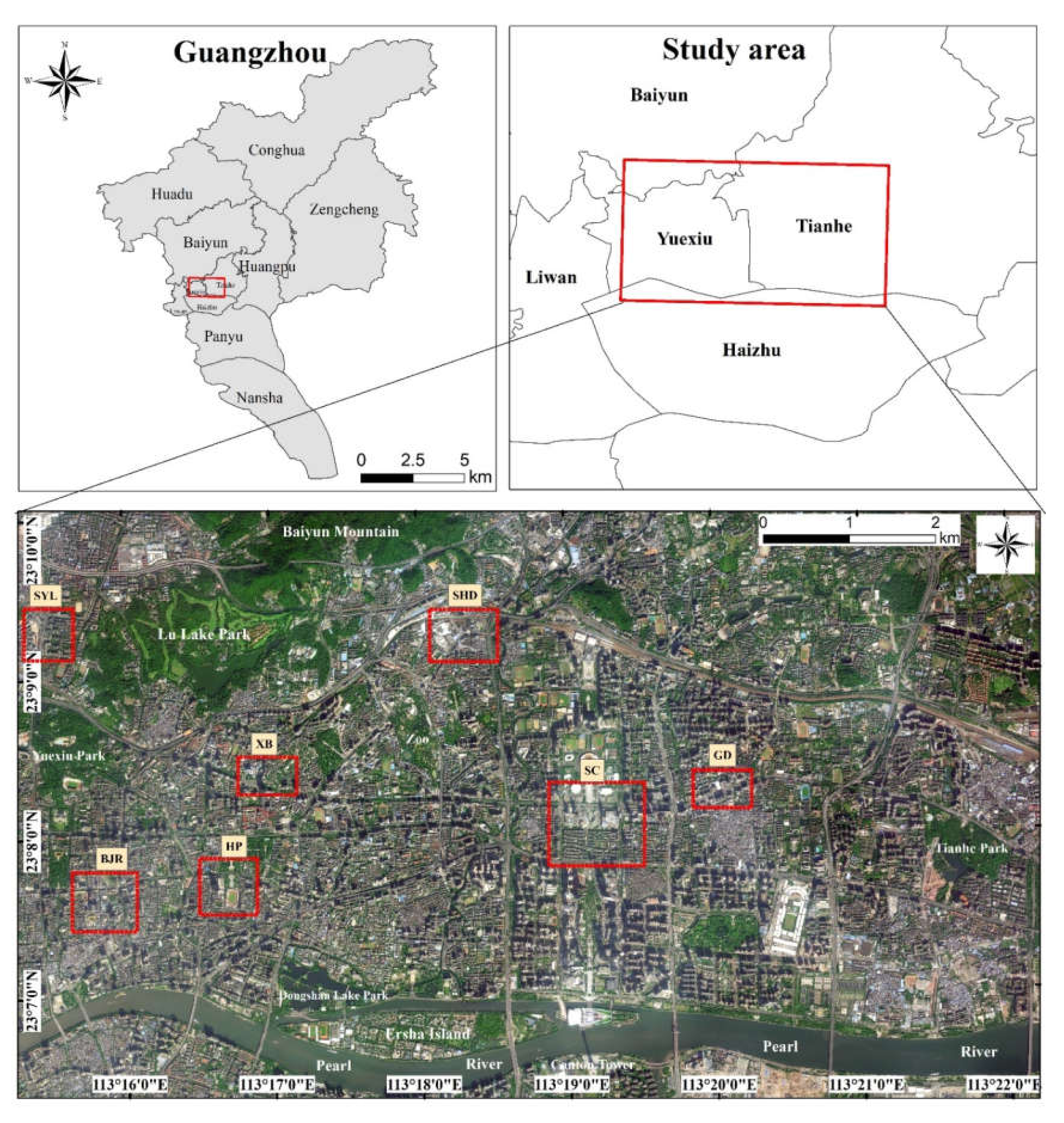
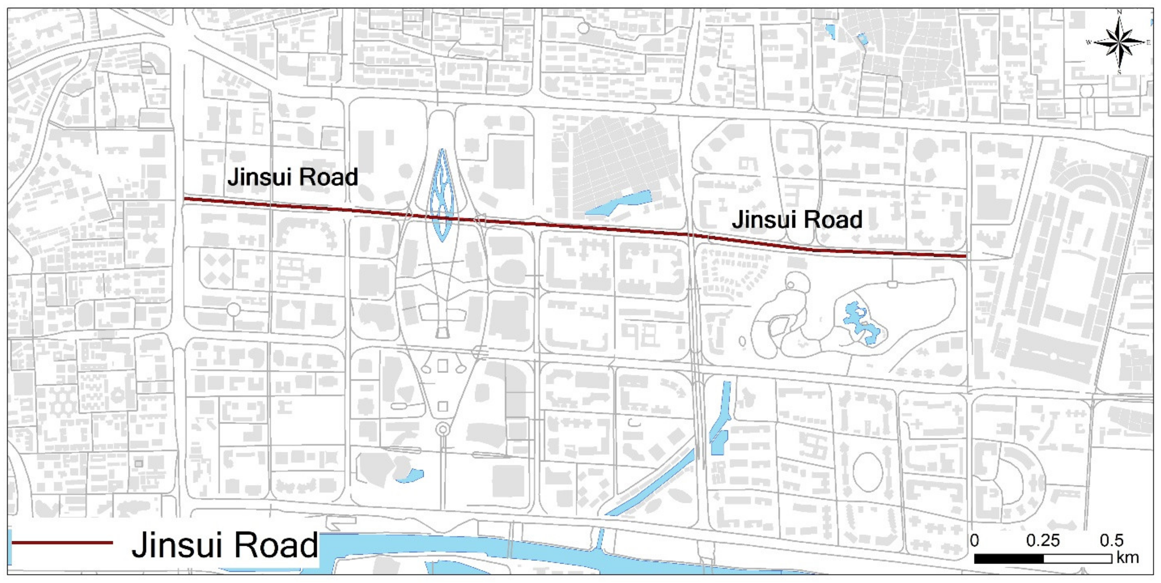
2.1. Study Area and Data Sources

Guangzhou city is the economic and cultural capital of Guangdong province located in southern China. It is the core city of the Guangdong–Hong Kong–Macao Greater Bay Area (GBA). The population in Guangzhou is close to 15 million, with a Gross Domestic Product (GDP) of 2.28 trillion Yuan in 2018. The study area is located in the center of Guangzhou, an area that contains Tianhe and Yuexiu districts, and several business districts, such as Sanyuanli Business District (SYL), Shaheding Business District (SHD), Xiaobei Business District (XB), Beijing Road Business District (BJR), Hero Plaza Business District (HP), Sport Center Business District (SC), and Gangding Business District (GD) (Figure 1). This area is the most prosperous region in Guangzhou, with the most retail stores, shopping malls, and restaurants. It is thus meaningful to examine the differences between shopping and dining street environments in this area.
POI data and remotely sensed data were employed to construct the shopping and dining oriented street indices. The POI data, which include the shopping malls, retail stores, and all types of restaurants, were collected from Gaode map [40] in 2016. Gaode map, similar to Google maps, is a Chinese digital map, navigation, and location services provider. It provides an application programming interface (API) for developers to download the POI data. We developed a Python tool to download the POI data and converted them to georeferenced vector data using coordinate information. A scene from a GaoFen-2 multispectral image (4-m spatial resolution) acquired on 4 November 2016, was used to calculate the normalized difference vegetation index (NDVI) and normalized difference water index (NDWI). A scene from the Landsat 8 Thermal Infrared Sensor (TIRS, 30-m spatial resolution; cloud cover percentage: 0) acquired on 5 November, 2016, was employed to retrieve the land surface temperature. The GaoFen-2 and Landsat 8 images were selected in the month of November for two reasons: (1) Close image acquisition date. There is only a one-day gap between GaoFen-2 and Landsat 8. (2) Image quality. There are few high-quality Landsat 8 and GaoFen-2 images during the spring and summer seasons, which are humid with frequent cloudy days. Street vector data and bus/subway station data were downloaded from Open Street Map (OSM) [41]. Street view images downloaded from Tencent map [42] was used to evaluate the walking environment of each street segment. All data were re-projected to the Universal Transverse Mercator Projection (UTM) in the zone 49N.

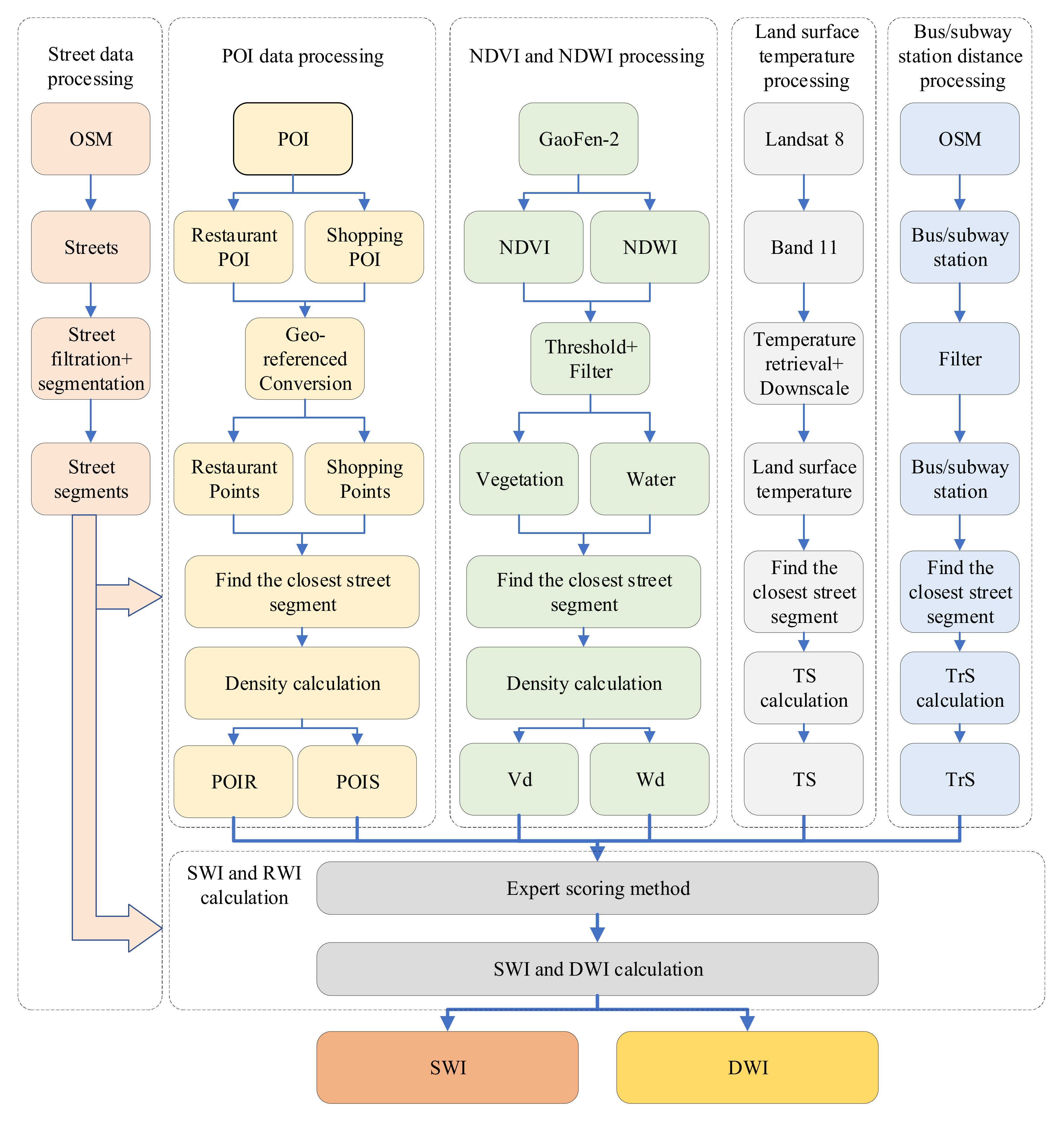
2.2. Index Construction

In this study, we employed six steps to construct a shopping walking index (SWI) and a dining walking index (DWI) with remote sensing data and POI data: (1) Street data processing (Section 2.2.1). The streets were split into 50-m-long segments and used for nearest feature selection and index construction. Street data were the basic data used for index construction. (2) POI data processing (Section 2.2.2). POI data were attached to the closest street segment, then POI density (restaurant density: POIR; shopping store POI density: POIS) of each street segment was calculated. (3) NDVI and NDWI processing (Section 2.2.3). NDVI and NDWI were calculated using GaoFen-2 imagery. Thresholds of NDVI and NDWI were set to distinguish vegetation and water, respectively. Vegetation and water points within a specified range were attached to the closest street segment. Vegetation density (Vd) and water density (Wd) were calculated for each street segment. (4) Land surface temperature processing (Section 2.2.4). Land surface temperature was inverted using Landsat 8 Thermal Infrared Sensor (TIRS). Then, the average land surface temperature of a street segment was calculated using image cells within a specified range. Finally, a categorized scheme was applied to calculate the temperature score (TS). (5) Bus/subway station distance processing (Section 2.2.5). A bus/subway station within 1500 m of a street segment was selected. Then, a transport score (TrS) was calculated using the linear distance function. (6) SWI and RWI calculation (Section 2.2.6). SWI and RWI of each street segment were calculated using POIR, POIS, Vd, Wd, TS, and TrS with the expert scoring method (see Figure 2).

2.2.1. Street Data Processing

Street vector data were filtered in this study before index construction. Highways, freeways, expressways, tunnels, bridges, and trunk roads that pedestrians cannot access were deleted. Footways, residential roads, secondary roads, service roads, and other roads that people can walk on were kept for evaluation. For streets longer than 1 km, this evaluation could only provide general information. For example, consider a street segment that is 300 m long: one-half of the street is covered by vegetation and provides access to POIs, while the other half is not suitable for pedestrians. Walking indices derived in previous research could only provide one value (likely the average of the whole environment) to evaluate this long street, and could thus not accurately reflect the conducive environment of the first half of the street (high concentration of vegetation and POIs) and the unsuitable environment of the other half (few vegetation or POIs). Therefore, each street is split into 50 m segments to present detailed street information.

2.2.2. POI Data Processing

Two types of POI data, restaurant and shopping POIs, were used in this study. Each type of POI also contains several sub-classes. Detailed subclass information is shown in Table 1. The collected POI data, which were stored in a text file, were geocoded using their X and Y coordinate information. Finally, these data were exported as a point shapefile with UTM projection information.
The Near function in ArcMap (ArcGIS) software (Environmental Systems Research Institute, ESRI) was used to determine the closest street for each POI point. Then, we summarized the frequency of POIs in each street segment. Lastly, the restaurant and shopping store POI density (POIR and POIS) were calculated using Equations (1) and (2), respectively:
POIR = ( Number   of   Restaurant   POI ) / ( Street   Segment   Length )
POIS = ( Number   of   Shopping   store   POI ) / ( Street   Segment   Length )

2.2.3. NDVI and NDWI Processing

The NDVI and NDWI were calculated from a GaoFen-2 multispectral image. The NDVI was computed using the near infrared band (NIR) and the red band (RED) [43], while the NDWI was calculated using the NIR and green band (GREEN) [44]. Derivation is shown in Equations (3) and (4):
NDVI = ( NIR RED ) / ( NIR + RED )
NDWI = ( GREEN NIR ) / ( GREEN + NIR )
where NDVI and NDWI are the normalized difference vegetation index and normalized difference water index, respectively. NIR, RED, and GREEN are the near infrared band, red band, and green band in the GaoFen-2 multispectral image.
The thresholds of NDVI and NDWI were set to extract the vegetation and water information. In total, 4652 samples of vegetation (V) and 3923 samples of non-vegetation (NV) were collected using the Worldview 2 image (with a spatial resolution of 0.5 m) to construct an NDVI frequency histogram (Figure 3). Higher NDVI value indicates more density of the vegetation. Thus, an NDVI value close to 1 implies high density vegetation while an NDVI value close to 0.1 indicates sparse vegetation. After careful examination, 0.1 was set as the threshold to distinguish V from NV. The overall accuracy of this threshold was 99%, meaning that only 27 of 8573 samples were misclassified. Thus, NDVI values larger than or equal to 0.1 were set as vegetation, while NDVI values less than 0.1 were set as non-vegetation and were deleted. For the water and non-water areas, we found that the major barrier to extracting water information was the confusion between water (W) and building shadows (S) (Figure 4). Similar to the method used to distinguish between vegetation and non-vegetation, 4011 samples of water and 4320 samples of shadows were collected from the NDWI results. A threshold of 0.199 was set for NDWI to distinguish between water and shadows. The overall accuracy of this threshold was 96%, meaning that 8014 of 8331 samples were classified correctly. Thus, the NDWI values larger than or equal to 0.199 were set as water. The NDWI values less than 0.199 were set as shadows and removed. The remaining vegetation and water cells (pixels) were converted into vector points using the center point of each cell with the ArcMap software. Since only some streets have center lines, and these streets are commonly more than 30 m wide, we set a buffer zone of 15 m (30/2 m) from the street’s center line for vegetation. Vegetation cover that is outside of the 15-m buffer zone was not taken into consideration. The water areas are slightly further away from the street than the vegetation. Thus, a 20-m buffer zone was set for the water area. Finally, the NDVI points completely within 15 m of a street and the NDWI points completely within 20 m of a street were retained, while the other NDWI and NDVI points were deleted.
The remaining vegetation and water points were assigned to the closest street segment using the ArcMap Near model. As a result, each vegetation and water point included the closest street segment’s FID (Feature identification). Then, we summarized each street segment’s FID in the vegetation and water point results to acquire the amount of vegetation and water in each street segment. Finally, the number of vegetation points, the number of water points, and the lengths of the corresponding street segments were employed to calculate the vegetation density (Vd) and water density (Wd). The vegetation and water density are viewed as vegetation cover and water cover. The detailed calculations are expressed in Equations (5) and (6):
Vd = ( Number   of   vegetation   point ) / ( Street   Segment   Length )
Wd = ( Number   of   water   point ) / ( Street   Segment   Length )
where Vd is the vegetation density and Wd is the water density.

2.2.4. Land Surface Temperature Processing

The original land surface temperature was inverted using the atmospheric correction method radiative transfer equation in the single channel algorithm with Band 11 in the Landsat 8 Thermal Infrared Sensor (TIRS) (for more details see [45,46,47]). Then, the land surface temperature was downscaled to a 10-m spatial resolution using a geostatistical method, the kriging model, and the impervious surface fraction, vegetation fraction, soil fraction, NDVI, normalized difference building index (NDBI) [48], NDWI, digital elevation model (DEM) [49], and building density. The impervious surface fraction can be calculated using the spectral mixture model for the Landsat 8 Operational Land Imager (OLI, 30-m spatial resolution) multispectral images. The detailed land surface temperature retrieval processing method is provided in Xu et al. (2020) [50]. Similar to the vegetation preprocessing method, the temperature cells beyond a 15-m range of the closest streets were deleted. The remaining temperature cells were converted into vector points with their corresponding values. The average temperature values of the remaining points were viewed as the land surface temperature of the relevant street segments.
The setting of the temperature score was based on the temperature range [51,52,53]. In this study, a temperature decay function was employed to separate the temperature range. We set the temperature score as 0 in a range between 18 and 23 °C, which is a suitable temperature range for walking. When the temperature is higher than 23 °C or less than 18 °C, the temperature score is set as (temperature−23) × 0.1 or (18–temperature) × 0.1, respectively, because we aimed to present the detailed difference of higher or lower temperatures outside the range of 18 to 23 ℃. The detailed temperature score was calculated using Equation (7):
TS = ( tem 23 ) × 0.1 ,   tem > 23 0 ,   18 < tem < 23 ( 18 tem ) × 0.1 ,   tem < 18
where TS is the temperature score and tem indicates the retrieved temperature in degrees Celsius. tem means land surface temperature.

2.2.5. Bus/Subway Station Distance Processing

The distance of bus/subway stations to each street segment is another element for consideration because the streets were split into 50-m segments, and some non-walking segments were deleted. The continuity of the street was broken, making it impossible to calculate the network distance. Therefore, we used the linear line distance to approximately estimate the distance between the bus/subway station and the street segment. Since the average speed of walking is 120 m/min [54], it would take about 12.5 min to walk 1500 m, which is unacceptable when looking for a shopping store or restaurant after getting off a bus or a subway. Thus, the street segments within a 1500 m buffer of a bus/subway station were assigned a positive score, while street segments outside the buffer (>1500 m) were assigned zero as their transport score.
In this study, we assumed that a linear function can represent a change of distance with more detail. Thus, we used a linear function to represent the change of distance instead of the distance decay function that has previously been employed in the walking score [19,23,25,55]. The transport score (TrS) was calculated using the linear distance function shown in Equation (8):
TrS = ( 1500 dis ) / 1500
where TrS is the transport score, and dis is the distance between a street segment and its closest bus/subway station. If a shopping store or restaurant is located close to a bus/subway station, that POI will have a transportation score closer to 1. On the other hand, if a segment is 1500 m away from a bus/subway station, the transportation score will be zero.

2.2.6. SWI and DWI Calculation

After calculating the POI density, vegetation coverage, water coverage, subway/bus station distance (transport score), and temperature, we constructed the shopping and dining walking indices. The walking index was constructed using five variables, namely, the street segment-based POI density (restaurant density or shopping point density), vegetation density, water density, transport score (distance to bus/subway station), and average temperature (Figure 4). Expert scoring methods were employed to assign weighting scores to different variables. The detailed weighting scores are shown in Table 2.
Since we aimed to emphasize the purpose of walking, the POI density variable was assigned the highest weighting score of 0.6. Tree shadows can provide a cooling effect for pedestrians in the summer [56]. Other vegetation types can also beautify the landscape in urban areas. Thus, we set the second highest weighting score of 0.3 to vegetation density. Water density also has a cooling function and ornamental value, as pedestrians feel comfortable when they walk around a water area. Hence, we set 0.1 as the weighting score for water. The weighting value for bus/subway station distance was set to 0.1 because we assumed that the influence of walking distance was smaller than the impact of the walking environment (vegetation density) and walking purpose (POI density). Extremely hot and cold temperatures make pedestrians feel uncomfortable. Therefore, the weighting score for temperature was negative (−0.1) in this study. The resulting shopping walking index (SWI) and dining walking index (DWI) are expressed in Equation (9) and Equation (10), respectively:
SWI = POIs × 0.6 + Vd × 0.3 + Wd × 0.1 + TrS × 0.1 TS × 0.1
DWI = POIr × 0.6 + Vd × 0.3 + Wd × 0.1 + TrS × 0.1 TS × 0.1

2.3. Walking Index Category Definition

The different walking index categories were defined based on degrees of recommendation. When the walking index is less than or equal to zero, the relevant POI type does not exist (no shopping store or restaurant). In this case, we defined this category as Not available. The second category was set as Deprecated, with an index range between 0 and 0.2. In this category, the density of the POIs is very low, and the walking environment is very poor (no vegetation or water area, long distance to bus/subway station, and high temperature). Thus, this street segment is not recommended for shopping or dining. The walking index values in the third category were set between 0.2 and 0.4 for the recommendation level of Acceptable. In this category, there are few POIs, and the vegetation and water cover is low. The fourth category is Recommended, with a walking index ranging from 0.4 to 0.6. Here, there are some POIs with a medium density of vegetation or water cover. A bus/subway station is not very far but also not close. The temperature is suitable. The remaining three categories are very suitable for shopping or dining. They have a high density of POIs and a good walking environment, such as a high density of vegetation and water cover, a short distance to a bus/subway station, and suitable temperature. A higher category indicates a better shopping and dining environment. Detailed information about all of the categories is shown in Table 3.

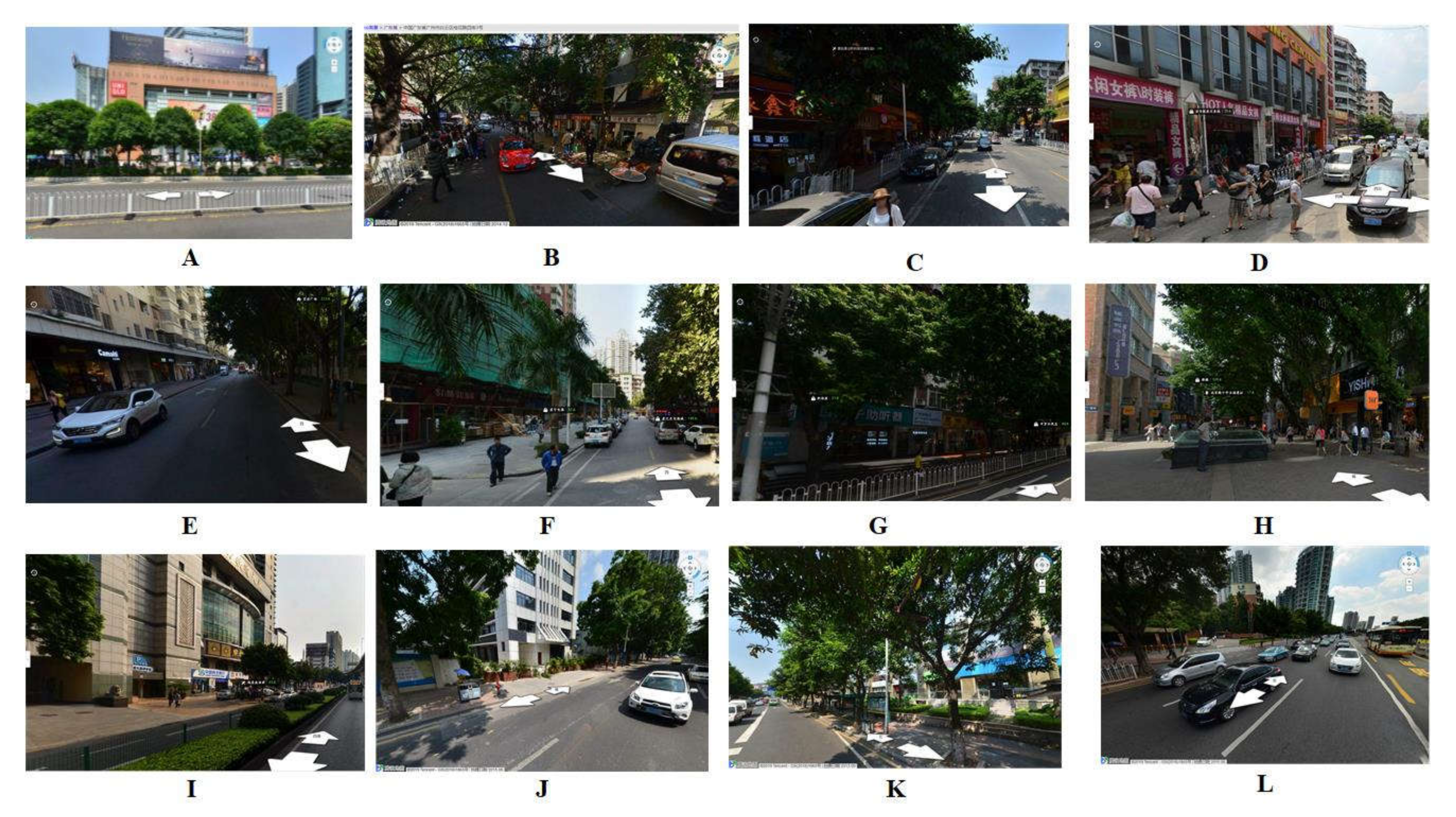
2.4. Field Validation

We randomly selected 12 sites to verify the accuracy of the two walking indices. A qualitative analysis and visual examination using street view images of Tencent map [42] was performed to evaluate the walking environment of each street segment. Street view images and field trip investigations were mainly used to assess the densities of the POIs, the vegetation cover, and the water area, and to analyze whether these densities match the walking index values. Then, three categories, including matching, partial matching, and mismatching, were assigned to each site to represent the degree of matching between the walking index value and reality. Matching indicates that the walking index value matches the real walking environment, while partial matching indicates that the walking index only matches part of the real walking environment. Mismatching suggests that the walking index value does not fully match the walking environment.

3. Results

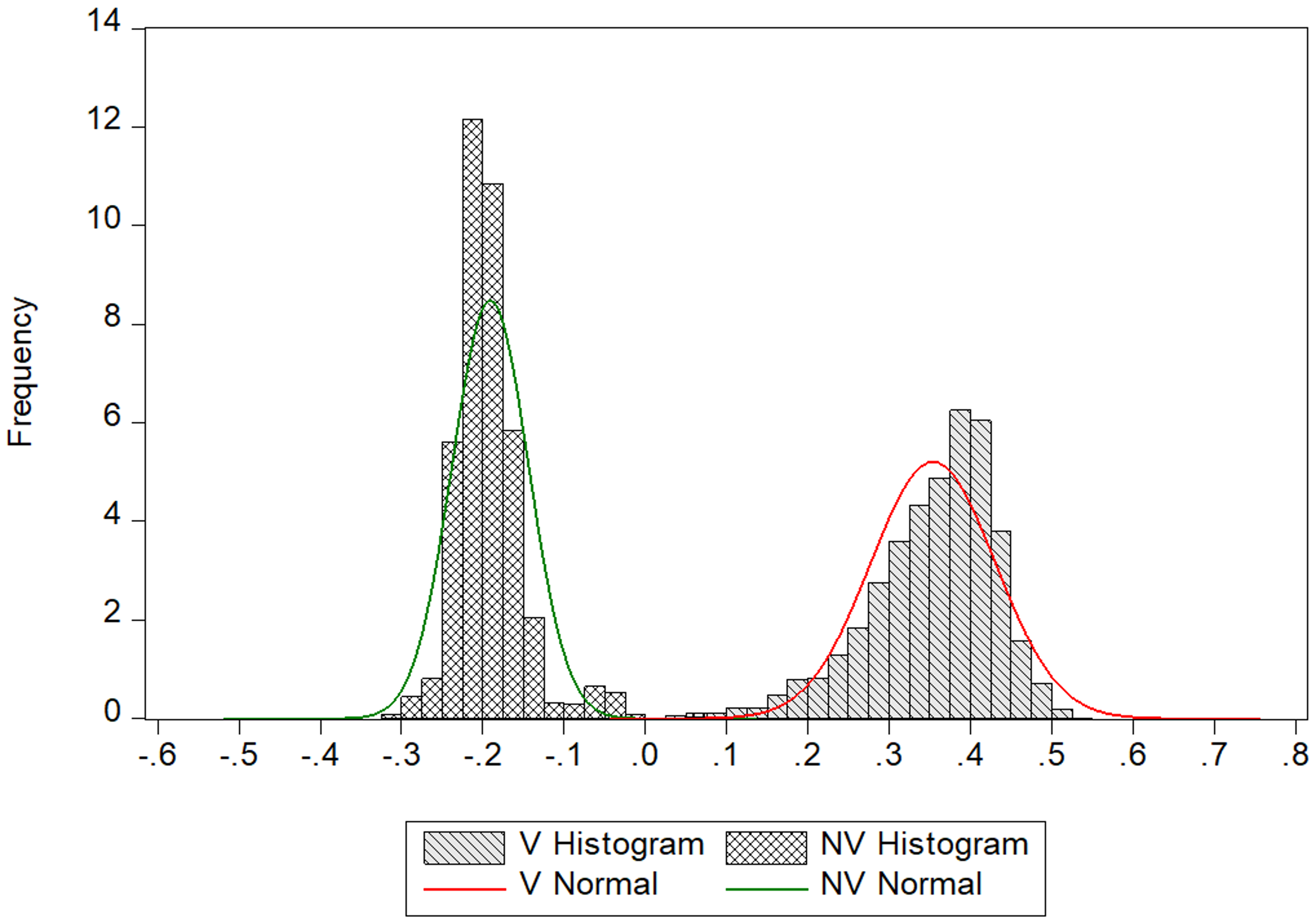
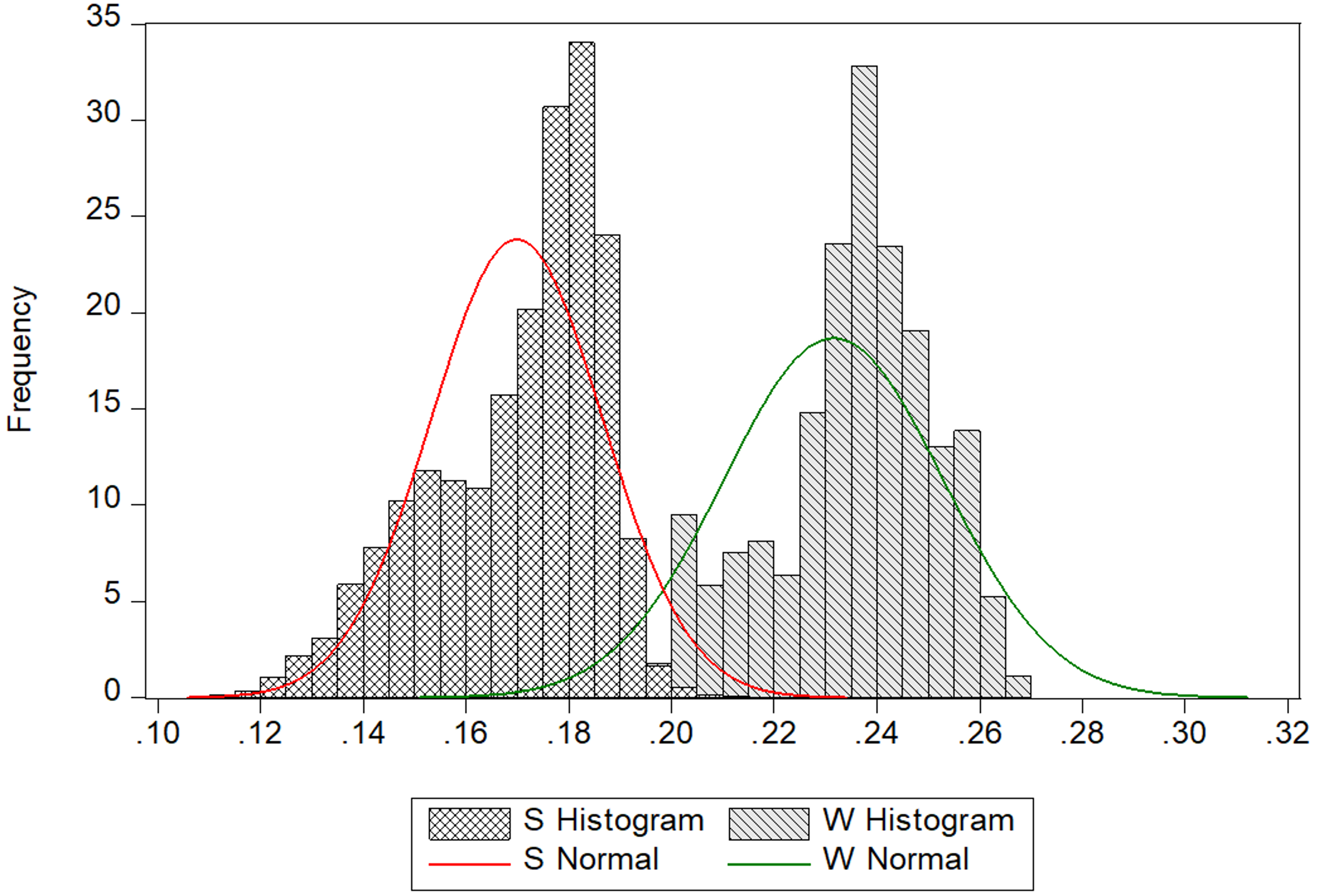
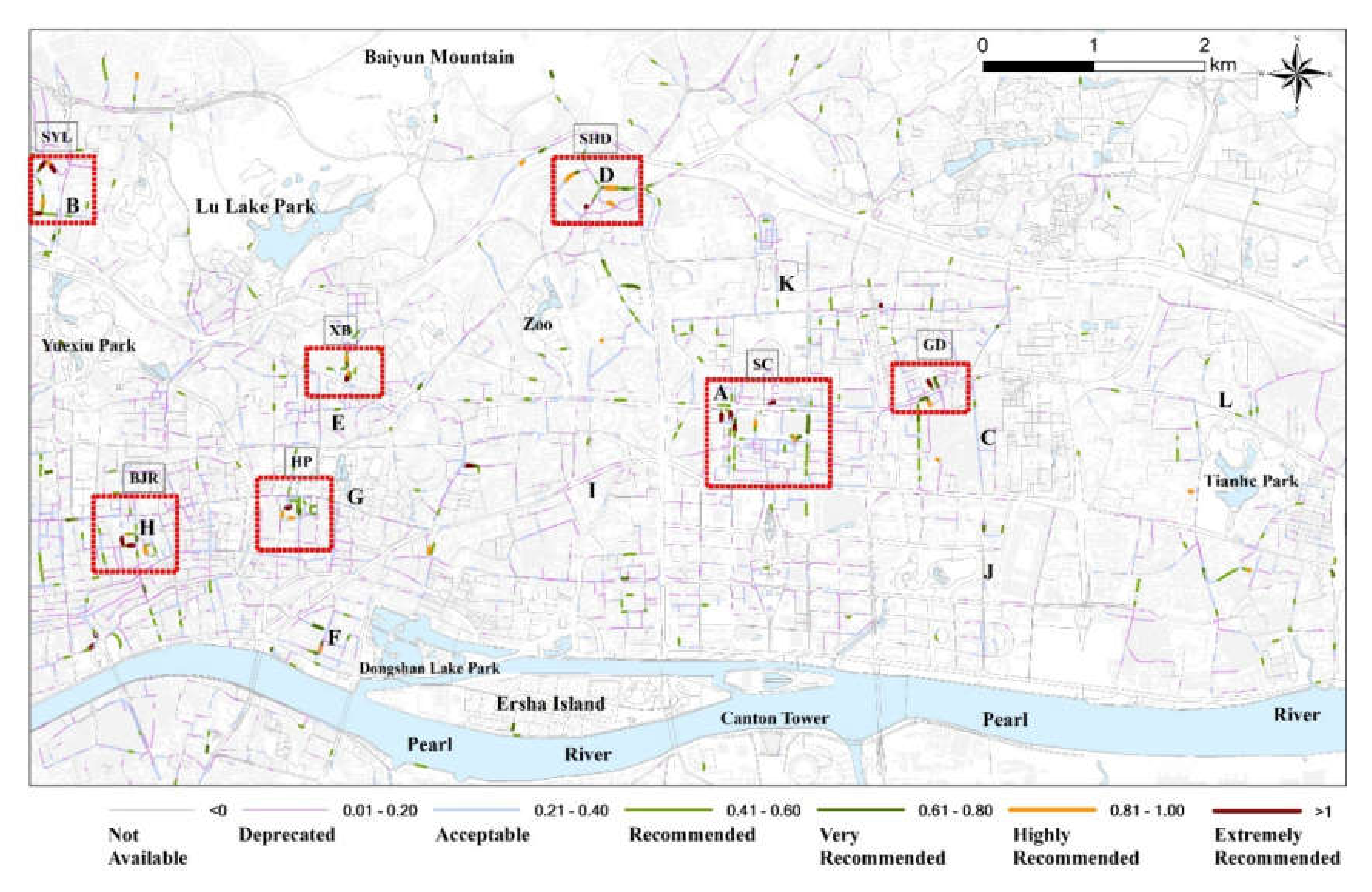
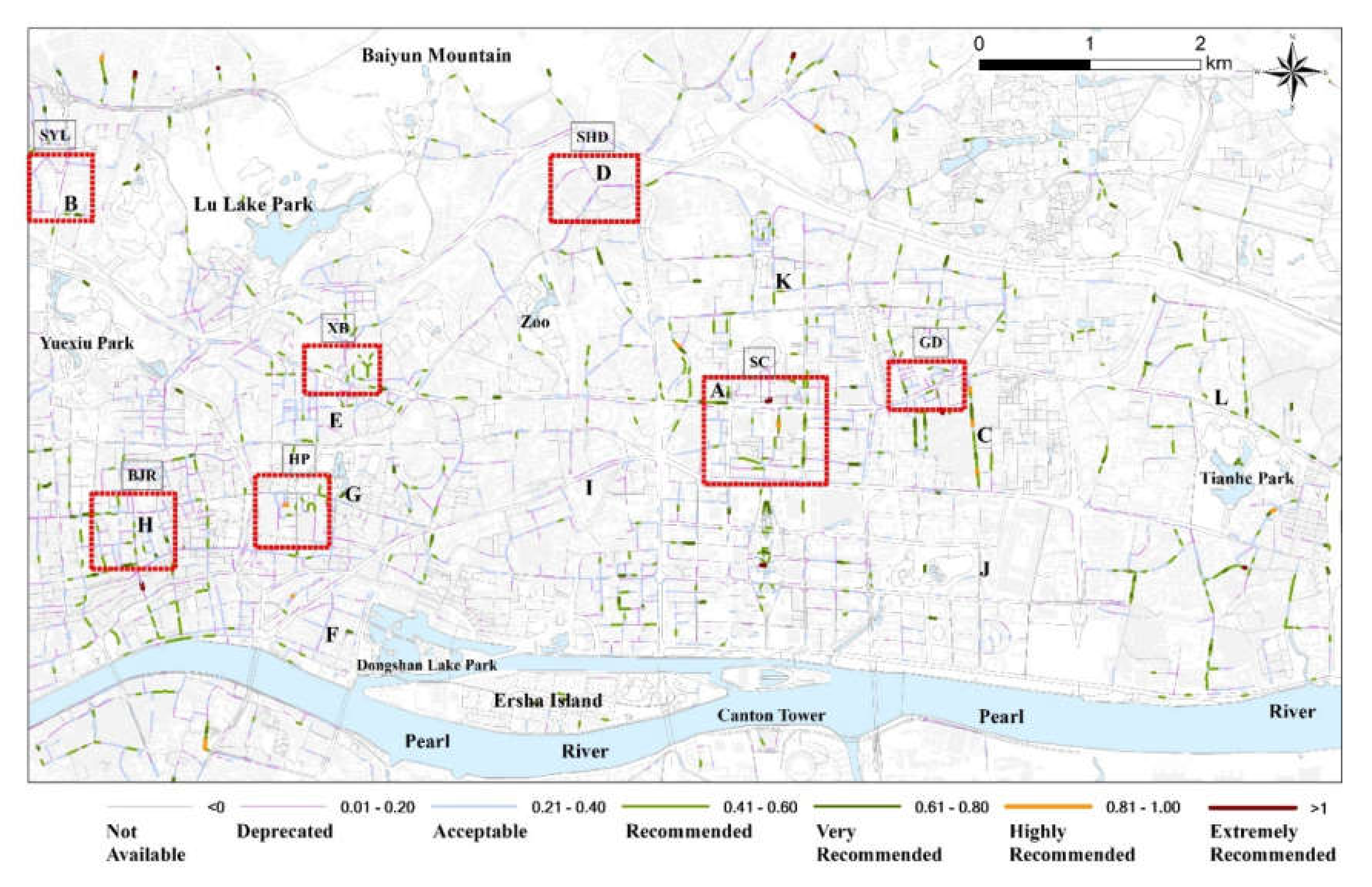
3.1. Shopping Walking Index (SWI)

The SWI represents a shopping-oriented walking environment (Figure 5). The results of the SWI show that there are only a few Extremely Recommended and Highly Recommended street segments located in the study area. Most of these high-category walking indices are clustered around popular business districts and shopping centers, such as Sanyuanli Business District (SYL), Shaheding Business District (SHD), Xiaobei Business District (XB), Hero Plaza Business District (HP), Gangding Business District (GD), Sport Center Business District (SC), and Beijing Road Business District (BJR). The number of Recommended and Very Recommended street segments is higher than the number of Highly Recommended and Extremely Recommended segments. Some segments are sparsely distributed outside the abovementioned major business districts. Most of the street segments in the study area are categorized as Acceptable. Figure 5 also illustrates that many streets are not suggested for shopping, such as the streets located around the parks (Lu Lake Park, Baiyun Mountain, Yuexiu Park) and residential areas (Ersha Island). These street segments may be better for leisure activities, such as walking exercises.

3.2. Dining Walking index (DWI)

The dining walking index (DWI) indicates the restaurant density and the related physical walking environment (Figure 6). The number of high DWI values (DWI > 0.8) is significantly less than the same category in the SWI. Few street segments can be categorized as Highly Recommended and Extremely Recommended, and some of these high category street segments were not located within the seven business districts mentioned in Section 3.1. The street segments in the Recommended and Very Recommended levels are both largely located within the business districts and other locations, such as Shipai street near location C in Figure 6. Low category DWI values (DWI < 0.4) are predominantly distributed around parks and residential areas (location J: park; Ersha Island: residential area).

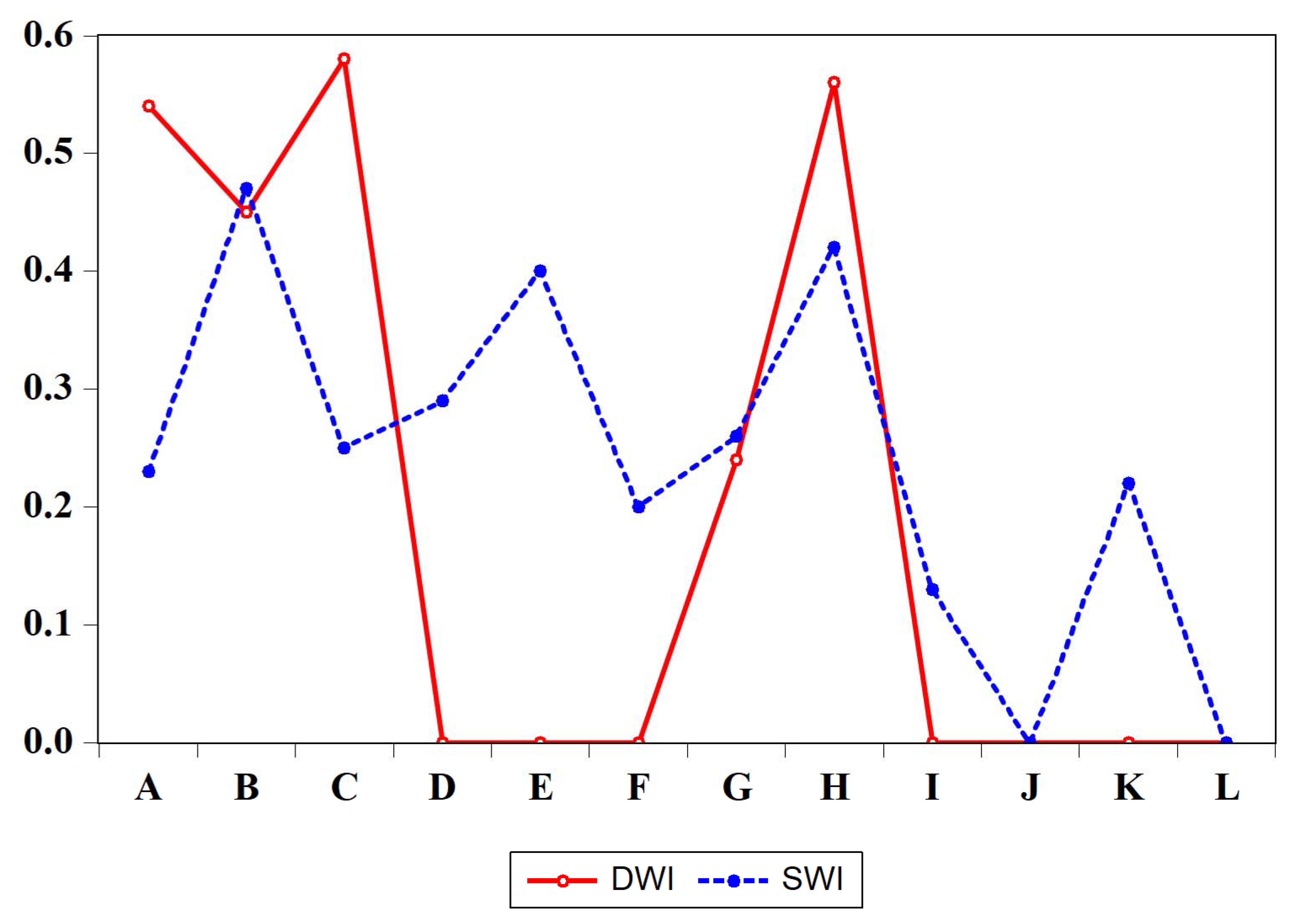
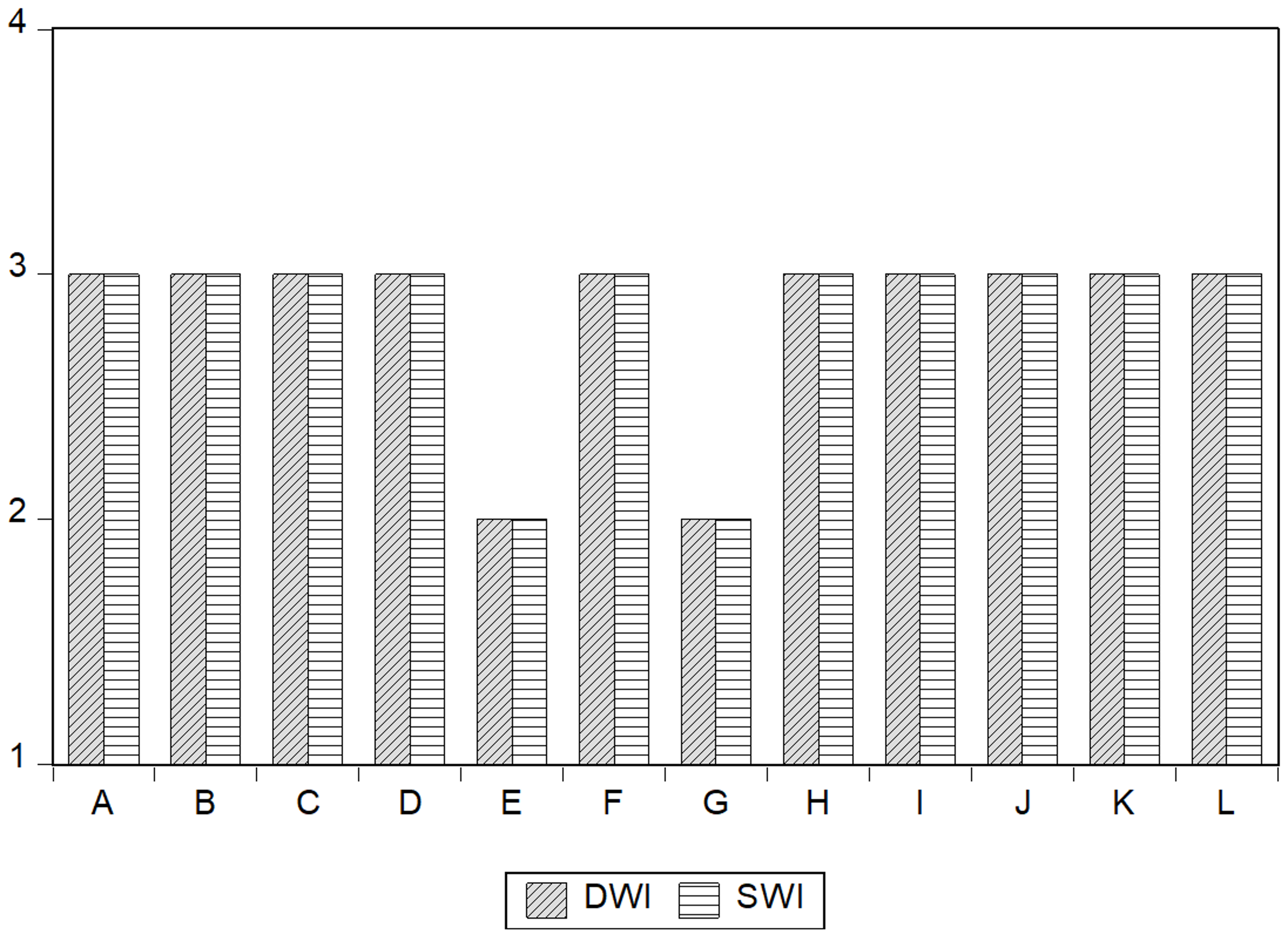
3.3. Field Validation Results

In order to evaluate the accuracy of the SWI and DWI, 12 street segments that have different scores were randomly selected from the study area (Figure 7, Figure 8 and Figure 9). Each street segment was evaluated from street view images and field trip verifications. Different levels of accuracy, including matching, partial matching, and mismatching, were assigned to each verified street segment. In this study, we only examined the number of POIs (shopping POIs and restaurant POIs), water cover, and vegetation cover. The land surface temperature was not examined since the acquisition date was different. Furthermore, the distances of bus/subway stations were not measured at this time. In Table 4, “Model calculation” comprises the parameters used for walking index construction, while “Field trip examination” are parameters counted by field trip and street view images. For the number of POIs (SPF: Shopping POI Frequency; RPF: Restaurant POI Frequency), we counted the number of the corresponding street segments during the field trip and through Gaode maps. It was hard to assess the WPFs (Water Point Frequency) and VPFs (Vegetation Point Frequency), so we estimated their frequency using high-spatial-resolution images and visual examination in the field. The accuracy assessment illustrated that 10 of the 12 sites matched the real walking environments (Figure 8 and Figure 9). Only two sites (E and G) acquired partial matching since they all overestimated the SWI and DWI. At site E, the vegetation was overestimated compared to the VPF in Table 4 and the street view image in Figure 7. In addition, the water area was located in a residential community where it could not be seen by pedestrians. Although it was not overestimated, the WPF could not reflect the true environment. Therefore, the SWI and DWI do not match the true walking environment perfectly at site E. At site G, it can be sees that the walking environment is suitable for pedestrians, with a high vegetation cover. However, the number of shopping stores and restaurants are underestimated (Table 4). After the field trip investigation, we verified that there are three restaurants (Badaoming Restaurant, Changlai Restaurant, and Sinkafee restaurant) and five shopping stores at site G. The numbers of SPF and RPF in the model are less than those in the field examination. Thus, the SWI and DWI are underestimated in site G.

4. Discussion

4.1. SWI and DWI Construction

This study proposed using a shopping walking index (SWI) and dining walking index (DWI) to evaluate shopping and dining-oriented street environments. The SWI and DWI were constructed based on the POI, the physical walking environment (vegetation and water cover), the distance to bus/subway stations, and the land surface temperature. The SWI focuses on shopping, while the DWI centers on restaurants.
The POI data collected from Baidu map are the primary source used to evaluate the distribution of urban facilities. Since the SWI and DWI are shopping- and dining-oriented, respectively, their POIs are the most important variable for constructing the indices. Unlike the walking score, our proposed walking indices only considered the shopping and dining POIs. The walking score, which aims to promote walkable neighborhoods [19], also uses these POIs to calculate its index. However, this score focuses more on the living neighborhoods in the community where there are restaurants, grocery stores, schools, parks, etc. [55]. The neighborhood community quality can be evaluated by the walking scores of given areas or streets. However, to find a specific place for shopping or dining, the walking score may not provide sufficiently detailed information.
Vegetation and water cover are two other variables used in this study, since these two types of land cover may affect the walking environment [57]. Guangzhou’s temperature is high, and its sunshine is very strong in the summer (from May to September) [58]. Vegetation and water cover can provide a cool space for pedestrians, which may increase their willingness to walk for shopping or dining [38,59]. High-spatial-resolution remotely sensed images provide a quick way to estimate vegetation and water cover using NDVI and NDWI [60]. These methods, however, are relatively simple and can also provide comparable vegetation water cover results via multispectral high-resolution images [61].
An important assumption in this study is that consumers will travel by public transportation, which is a form of green travel [62]. Thus, the distance to the bus/subway station is another key element for SWI and DWI construction. Referring to a previous study by Carr et al. 2010 [55], in which a 1600-m range was set for the Walk Score distance, we considered a distance within 1500 m. On average, it takes more than 12.5 min to walk 1.5 km; 12.5 min is not a long time when walking for leisure or excise. However, it may reduce consumers’ patience if they need to walk for 12.5 min to reach a shop or restaurant. Thus, with a linear decay function, street segments that are very close to bus/subway stations will have a score of 1, and segments that are 1500 m away from a bus/subway station will have a score of 0. Recently, researchers designed a distance score based on the road network [63,64]. This score may work well for a neighbor-based community in which citizens walk more than 1.5 km for leisure or work. The connectivity of the road provides great convenience for residents, but this may not hold true for consumers or travelers who aim to find a place for shopping or dinning. Thus, a network-based distance function is not employed in our study.
The land surface temperature extracted from Landsat thermal infrared bands is another element used to construct SWI and DWI [65]. Temperature, especially in summer, is one of the key factors that affects a citizen’s willingness to go outside. Thus, it is necessary to take the temperature into consideration. However, the air temperature is hard to measure. Thus, in this study, we used the land surface temperature to approximately estimate the air temperature. This is one of the major differences between our method and other walkability indices, which do not employ temperature to evaluate the walking score [19,23].
The impact of seasonal variation on walking index construction is limited. The number of POIs is stable within a year. It is inevitable that stores and restaurants will change their locations to look for the best locations. However, this is also a long-term process. It is unreasonable to expect stores and restaurants to change their location in the short-term; because relocation likely requires spending a large amount of money for decoration, changing location frequently may be expensive and result in higher operating costs. Therefore, the change in the number of POIs has limited impact on the calculation of the DWI and SWI within the period of a year.
Water and vegetation density change little during a year. This study area is located in the subtropical monsoon climate zone. Evergreen broad-leaf forest is the major vegetation type, which changes little due to seasonality. Similarly, grass and shrubs are nearly constant in different seasons. Therefore, the change of NDVI is limited in this study area, resulting in limited change of Vd in different seasons. Similar to the vegetation cover, the change of water area is also limited. The major water areas are rivers and lakes in the parks. These water areas change little in different seasons. Therefore, the change of Wd is also limited.
Generally, there is no significant change in the number of bus/subway stations within a year. Clearly, more bus/subway stations will be built in the future. However, this will occur over a long period and change within a year is limited. As a result, distance to bus/subway station varies within a limited range within a year. Thus, DWI and SWI are affected to a limited degree by the distance to bus/subway stations.
Temperature obviously varies from season to season. In the study area, summer is characterized by high temperature and high humidity, while winter is cool and comparatively dry. The average daytime temperature in summer is higher than 30 °C, which is outside the range of 18–23 ℃. Thus, the walking indices are lower in summer than in winter, since the TS value is larger in summer and its weighting score is negative in the model. Thus, the DWI and SWI values change depending on the season because of the temperature variation. Nonetheless, the change of TS is within a small range. If, for example, the temperatures of a street segment are 32 and 20 ℃ in summer and winter, respectively, their TSs will be 0.9 and 0 according Equation (7). Moreover, since the weight score of TS is −0.1, the contribution of TS for walking index in summer is 0.09 compared to 0 in winter. Therefore, although temperature variation can affect the DWI and SWI, its impact is nonetheless limited to a small range.
The DWI and SWI can be applied in other urban areas using the same index construction scheme. However, some parameters would need to be revised in a new study area: (1) The thresholds of NDWI and NDVI. Since atmospheric environments differ, the NDWI and NDVI values may vary in different time periods and locations. Thus, new water and vegetation samples would need to be collected to design the thresholds of NDWI and NDVI. (2) The distance to bus/subway station. The DWI and SWI are designed for a flat area and, thus, may not be appropriate for mountainous terrain. Since the bus/subway distance is calculated based on the two-dimensional straight-line distance, it is not fit for mountainous terrain where the distance should be calculated based on a three-dimensional line.

4.2. Shopping and Dining-Oriented Walking Indices

Compared to the walking scores, the SWI and DWI place greater focus on the shopping, dining, and walking environment. The walking score assesses three different types of walking: purposeful walking, physical activity, and all types of walking [66]. However, SWI and DWI more strongly emphasize purposeful walking (shopping and dining) and the physical walking environment outside destinations. Shopping and dining are two activities that are strongly related to leisure time [39], and many consumers engage in shopping and dining together. However, the current walking score cannot satisfy these major purposes of consumers since such scores cannot provide specific suggestions for locations of relevant POIs that are within walking distance. However, if consumers look at the proposed walking indices, they can easily determine the most recommended street segments in the SWI results for shopping or dining. Our SWI and DWI can save consumers considerable time in finding these two types of locations, as well as a suitable walking environment. With the weighting score of POIs and the walking environment, our street indices primarily emphasize the purpose of walking followed by the walking environment, simultaneously satisfying the walking purpose and comfort.

4.3. 50-m Street Segment

Another highlight of our study is our focus on providing detailed information of a street segment that is 50 m long. Most current studies analyze the whole street as an individual object [23,27]. Some streets in Guangzhou, such as Jinsui road (Figure 10), have a length of more than 2 km, and their subsegments in a block are more than 500 m long. Such a long segment can only provide general information for a street. This general information may cause confusion if a consumer wants to find a place with many options for shopping or dining, thus wasting considerable time. Cutting these long roads into 50-m segments enables consumers to easily identify the clustered shopping and dining segments. The 50-m-long street segment can reduce the confusion in finding potential stores or locations. This is one of the major advantages of SWI and DWI compared to the walking score. We focused on the detailed information in each 50-m segment of a street to decrease the time needed to find potential destinations. Of course, a heat map created by density functions can also present hot spot areas [67]. However, it cannot present the street’s physical environment, such as its vegetation cover, water area, and the distance to bus/subway stations. Thus, the shopping and dining-oriented walking environment cannot be accurately provided by a heat map.
Two sites (E and G) were overestimated in this study. For E, there is a water area in the residential area that contributes 10% to the walking index. However, this water area is located in a residential area that pedestrians cannot access directly. In the future, more data, such as land use and land cover types, should be used to avoid situations like that of site E. For site G, we closely examined the values of each variable, and found that the distance to the bus/subway station is short, the vegetation cover is very high, and the LST is low, contributing more than 40% to the final walking index. Thus, to some degree, this walking index value can still represent a real shopping or dining environment.
This study constructed two walking indices: one for shopping- and one for dining-oriented walking. However, some limitations remain that need to be solved in future studies. The type of shopping/dining should be detailed to provide more specific information. For example, it may be useful to set various categories for different types of restaurants/shopping. Assigning different weights to each shopping/dining type in the model may provide more precise shopping and dining information for these two indices. The bus/subway distance calculation method also needs to be improved in the future. A network-based distance calculation may provide a more accurate walking distance from the bus/subway station to the desired destination. Moreover, the slope and other landscape parameters should be taken into consideration in the future because the slope can affect the speed and comfort level of walking [68]. More parameters, such as distance to vegetation and water, and fuzzy logic computation methods, will be considered in future work to make the model more robust. Finally, subcategories related to consumers, such as parents with children and people with limited walking abilities, will be taken into consideration in future studies.

5. Conclusions

This study proposed two walking indices, namely, a shopping walking index (SWI) and a dining walking index (DWI), to evaluate shopping- and dining-oriented walking environments. The SWI and DWI were constructed using the relevant POIs (SWI: shopping, DWI: restaurants), vegetation cover, water area, bus/subway station distance, and land surface temperature. An expert scoring method that assigns different scores to each element was employed, not only to emphasize the importance of the POIs, but also to focus on the walking environment of the street. The SWI and DWI were categorized into seven levels to provide a visualized suggestion to help customers determine the best option for shopping or dining. The accuracy assessment showed that most of the SWI and DWI values matched the real situation of a street segment.

Author Contributions

Conceptualization, Yingbin Deng and Yingwei Yan; methodology, Yingbin Deng, Yichun Xie, and Runnan Tan; validation, Renrong Chen; formal Analysis, Jianhui Xu; resources, Hao Jiang; writing—original draft preparation, Yingbin Deng; writing—review and editing, Yichun Xie; funding acquisition, Yingbin Deng and Yingwei Yan. All authors have read and agreed to the published version of the manuscript.

Funding

This research was funded by the GDAS Project of Science and Technology Development, China [2019GDASYL-0103004, 2020GDASYL-20200103005]; National Natural Science Foundation of China [41901372 and 41901330]; Key Special Project for Introduced Talents Team of Southern Marine Science and Engineering Guangdong Laboratory (Guangzhou) [GML2019ZD0301]; and Guangdong Innovative and Entrepreneurial Research Team Program(2016ZT06D336).

Acknowledgments

The authors would like to thank the Team of Ying Long and his Lab (Beijing City Lab) for providing the walking score data of Guangzhou; we would also like to thank the anonymous reviewers for their constructive comments.

Conflicts of Interest

The authors declare that there are no real or perceived conflicts of interest involved in the submission and/or publication of this manuscript.

References

  1. D’Orso, G.; Migliore, M. A GIS-based method for evaluating the walkability of a pedestrian environment and prioritised investments. J. Transp. Geogr. 2020, 82, 102555. [Google Scholar] [CrossRef]
  2. WHO. Global Recommendations on Physical Activity for Health; World Health Organization: Geneva, Switzerland, 2010. [Google Scholar]
  3. De Vries, S.; Van Dillen, S.M.; Groenewegen, P.P.; Spreeuwenberg, P. Streetscape greenery and health: Stress, social cohesion and physical activity as mediators. Soc. Sci. Med. 2013, 94, 26–33. [Google Scholar] [CrossRef]
  4. Howell, N.A.; Tu, J.V.; Moineddin, R.; Chen, H.; Chu, A.; Hystad, P.; Booth, G.L. Interaction between neighborhood walkability and traffic-related air pollution on hypertension and diabetes: The CANHEART cohort. Environ. Int 2019, 132, 104799. [Google Scholar] [CrossRef] [PubMed]
  5. Council, N.R. Driving and the Built Environment: The Effects of Compact Development on Motorized Travel, Energy Use, and CO2 Emissions—Special Report 298; National Academies Press: Washington, DC, USA, 2010. [Google Scholar]
  6. Geng, J.; Long, R.; Chen, H.; Li, W. Exploring the motivation-behavior gap in urban residents’ green travel behavior: A theoretical and empirical study. Resour. Conserv. Recycl. 2017, 125, 282–292. [Google Scholar] [CrossRef]
  7. Wang, Z.; Liu, W. Determinants of CO2 emissions from household daily travel in Beijing, China: Individual travel characteristic perspectives. Appl. Energy 2015, 158, 292–299. [Google Scholar] [CrossRef]
  8. Duncan, D.T.; Aldstadt, J.; Whalen, J.; White, K.; Castro, M.C.; Williams, D.R. Space, race, and poverty: Spatial inequalities in walkable neighborhood amenities? Demogr. Res. 2012, 26, 409. [Google Scholar] [CrossRef] [Green Version]
  9. Cortright, J. Walking the Walk: How Walkability Raises Home Values in US Cities; CEOs for Cities: 2009. Available online: https://community-wealth.org/sites/clone.community-wealth.org/files/downloads/report-cortright.pdf (accessed on 1 June 2019).
  10. Zhu, W.; Nedovic-Budic, Z.; Olshansky, R.B.; Marti, J.; Gao, Y.; Park, Y.; McAuley, E.; Chodzko-Zajko, W. Agent-based modeling of physical activity behavior and environmental correlations: An introduction and illustration. J. Phys. Act. Health 2013, 10, 309–322. [Google Scholar] [CrossRef]
  11. Perrotta, K.; Campbell, M.; Chirrey, S.; Frank, L.; Chapman, J. The Walkable City: Neighbourhood Design and Preferences, Travel Choices and Health; Toronto Public Health: Toronto, ON, Canada, 2012. [Google Scholar]
  12. Giles-Corti, B.; Vernez-Moudon, A.; Reis, R.; Turrell, G.; Dannenberg, A.L.; Badland, H.; Foster, S.; Lowe, M.; Sallis, J.F.; Stevenson, M. City planning and population health: A global challenge. Lancet 2016, 388, 2912–2924. [Google Scholar] [CrossRef]
  13. Zhou, H.; He, S.; Cai, Y.; Wang, M.; Su, S. Social inequalities in neighborhood visual walkability: Using Street View imagery and deep learning technologies to facilitate healthy city planning. Sustain. Cities Soc. 2019, 50, 101605. [Google Scholar] [CrossRef]
  14. Bahrainy, H.; Khosravi, H. The impact of urban design features and qualities on walkability and health in under-construction environments: The case of Hashtgerd New Town in Iran. Cities 2013, 31, 17–28. [Google Scholar] [CrossRef]
  15. Yameqani, A.S.; Alesheikh, A.A. Predicting subjective measures of walkability index from objective measures using artificial neural networks. Sustain. Cities Soc. 2019, 48, 101560. [Google Scholar] [CrossRef]
  16. Park, S.; Deakin, E.; Lee, J.S. Perception-based walkability index to test impact of microlevel walkability on sustainable mode choice decisions. Transp. Res. Rec. 2014, 2464, 126–134. [Google Scholar] [CrossRef]
  17. Su, S.; Pi, J.; Xie, H.; Cai, Z.; Weng, M. Community deprivation, walkability, and public health: Highlighting the social inequalities in land use planning for health promotion. Land Use Policy 2017, 67, 315–326. [Google Scholar] [CrossRef]
  18. TRL. What Is PERS. Available online: https://trlsoftware.com/products/road-safety/street-auditing/streetaudit-pers/ (accessed on 21 April 2020).
  19. Walk Score C. Walk Score Methodology. Available online: https://www.walkscore.com/methodology.shtml (accessed on 21 April 2020).
  20. Duncan, D.T.; Aldstadt, J.; Whalen, J.; Melly, S.J. Validation of Walk scores and Transit Scores for estimating neighborhood walkability and transit availability: A small-area analysis. GeoJournal 2013, 78, 407–416. [Google Scholar] [CrossRef]
  21. Koschinsky, J.; Talen, E.; Alfonzo, M.; Lee, S. How walkable is Walker’s paradise? Environ. Plan. B Urban Anal. City Sci. 2017, 44, 343–363. [Google Scholar] [CrossRef]
  22. Gilderbloom, J.I.; Riggs, W.W.; Meares, W.L. Does walkability matter? An examination of walkability’s impact on housing values, foreclosures and crime. Cities 2015, 42, 13–24. [Google Scholar] [CrossRef]
  23. Long, Y.; Zhao, J.; Li, S.; Zhou, Y.; Xu, L. The Large-Scale Calculation of “Walk score” of Main Cities in China. New Archit. 2018, 3, 4–8. [Google Scholar]
  24. Jiansheng, W.; Shen, N. Walk score method-based evaluation of social service function of urban park green lands in Futian district, Shenzhen, China. Acta Ecol. Sin. 2019, 37, 7483–7492. [Google Scholar]
  25. Brown, S.C.; Pantin, H.; Lombard, J.; Toro, M.; Huang, S.; Plater-Zyberk, E.; Perrino, T.; Perez-Gomez, G.; Barrera-Allen, L.; Szapocznik, J. Walk score®: Associations with purpose walking in recent Cuban immigrants. Am. J. Prev. Med. 2013, 45, 202–206. [Google Scholar] [CrossRef] [Green Version]
  26. Litman, T.A. Economic Value of Walkability; Victoria Transport Policy Institute: Victoria, BC, Canada, 2017. [Google Scholar]
  27. Duncan, D.T.; Aldstadt, J.; Whalen, J.; Melly, S.J.; Gortmaker, S.L. Validation of Walking score® for estimating neighborhood walkability: An analysis of four US metropolitan areas. Int. J. Environ. Res. Public. Health 2011, 8, 4160–4179. [Google Scholar]
  28. Singleton, P.A.; Schneider, R.J.; Muhs, C.; Clifton, K.J. The pedestrian index of the environment: Representing the walking environment in planning applications. In Proceedings of the 93rd Annual Meeting, Transportation Research Board, Washington, DC, USA, 12–16 January 2014. [Google Scholar]
  29. Knapskog, M.; Hagen, O.H.; Tennøy, A.; Rynning, M.K. Exploring ways of measuring walkability. Transp. Res. Procedia 2019, 41, 264–282. [Google Scholar] [CrossRef]
  30. Kuzmyak, J.R.; Baber, C.; Savory, D. Use of walk opportunities index to quantify local accessibility. Transp. Res. Rec. 2006, 1977, 145–153. [Google Scholar] [CrossRef]
  31. Freeman, L.; Neckerman, K.; Schwartz-Soicher, O.; Quinn, J.; Richards, C.; Bader, M.D.; Lovasi, G.; Jack, D.; Weiss, C.; Konty, K. Neighborhood walkability and active travel (walking and cycling) in New York City. J. Urban Health 2013, 90, 575–585. [Google Scholar] [CrossRef] [PubMed] [Green Version]
  32. Frackelton, A.; Grossman, A.; Palinginis, E.; Castrillon, F.; Elango, V.; Guensler, R. Measuring walkability: Development of an automated sidewalk quality assessment tool. Suburb. Sustain. 2013, 1, 4. [Google Scholar] [CrossRef] [Green Version]
  33. Saelens, B.E.; Sallis, J.F.; Black, J.B.; Chen, D. Neighborhood-based differences in physical activity: An environment scale evaluation. Am. J. Public Health 2003, 93, 1552–1558. [Google Scholar] [CrossRef]
  34. Buck, C.; Tkaczick, T.; Pitsiladis, Y.; De Bourdehaudhuij, I.; Reisch, L.; Ahrens, W.; Pigeot, I. Objective measures of the built environment and physical activity in children: From walkability to moveability. J. Urban Health 2015, 92, 24–38. [Google Scholar] [CrossRef] [Green Version]
  35. Witten, K.; Pearce, J.; Day, P. Neighbourhood Destination Accessibility Index: A GIS tool for measuring infrastructure support for neighbourhood physical activity. Environ. Plan. A 2011, 43, 205–223. [Google Scholar] [CrossRef]
  36. Millstein, R.A.; Cain, K.L.; Sallis, J.F.; Conway, T.L.; Geremia, C.; Frank, L.D.; Chapman, J.; Van Dyck, D.; Dipzinski, L.R.; Kerr, J. Development, scoring, and reliability of the Microscale Audit of Pedestrian Streetscapes (MAPS). BMC Public Health 2013, 13, 403. [Google Scholar] [CrossRef] [Green Version]
  37. Cain, K.; Millstein, R.; Geremia, C. Microscale audit of pedestrian streetscapes (MAPS): Data Collection & Scoring Manual. University California San Diego. Available online: http://sallis.ucsd.edu/Documents/Measures_documents/MAPS%20Manual_v1_010713.pdf (accessed on 8 August 2013).
  38. Drake-McLaughlin, N.; Netusil, N.R. Valuing walkability and vegetation in Portland, Oregon. In Proceedings of the Twenty-Second Interim Report and Proceedings from the Annual Meeting, Benefits and Costs of Natural Resources Policies Affecting Public and Private Lands, New York, NY, USA, 14–18 June 2010; Volume 2, p. 173. [Google Scholar]
  39. Davis, A.W. Using Road Network Spatial Clustering to Assess the Timing and Duration of Dining, Shopping, and Entertainment Activities in California; UC Santa Barbara: Santa Barbara, CA, USA, 2019. [Google Scholar]
  40. Gaode Map. Available online: https://www.amap.com/ (accessed on 1 January 2016).
  41. Open Street Map. Available online: www.openstreetmap.org (accessed on 1 May 2020).
  42. Tencent Map. Available online: https://map.qq.com (accessed on 1 June 2020).
  43. Becker, F.; Choudhury, B.J. Relative sensitivity of normalized difference vegetation index (NDVI) and microwave polarization difference index (MPDI) for vegetation and desertification monitoring. Remote Sens. Environ. 1988, 24, 297–311. [Google Scholar] [CrossRef]
  44. Gao, B.-C. NDWI—A normalized difference water index for remote sensing of vegetation liquid water from space. Remote Sens Environ. 1996, 58, 257–266. [Google Scholar] [CrossRef]
  45. Jiménez-Muñoz, J.C.; Sobrino, J.A. A generalized single-channel method for retrieving land surface temperature from remote sensing data. J. Geophys. Res. Atmos. 2003, 108, 1–9. [Google Scholar] [CrossRef] [Green Version]
  46. Jiménez-Muñoz, J.; Sobrino, J. Error sources on the land surface temperature retrieved from thermal infrared single channel remote sensing data. Int. J. Remote Sens. 2006, 27, 999–1014. [Google Scholar] [CrossRef]
  47. Jiménez-Muñoz, J.C.; Cristóbal, J.; Sobrino, J.A.; Sòria, G.; Ninyerola, M.; Pons, X. Revision of the single-channel algorithm for land surface temperature retrieval from Landsat thermal-infrared data. IEEE Trans. Geosci. Remote Sens. 2008, 47, 339–349. [Google Scholar] [CrossRef]
  48. Yi, Z.; Jianhui, X. Impervious surface extraction with Linear Spectral Mixture Analysis integrating Principal components analysis and Normalized Difference Building Index. In Proceedings of the 4th International Workshop on Earth Observation and Remote Sensing Applications (EORSA), Guangzhou, China, 4–6 July 2016; pp. 428–432. [Google Scholar]
  49. Zhang, W.; Montgomery, D.R. Digital elevation model grid size, landscape representation, and hydrologic simulations. Water Resour. Res. 1994, 30, 1019–1028. [Google Scholar] [CrossRef]
  50. Xu, J.; Zhang, F.; Jiang, H.; Hu, H.; Zhong, K.; Jing, W.; Yang, J.; Jia, B. Downscaling ASTER land surface temperature over urban areas with machine learning-based area-to-point regression Kriging. Remote Sens. 2020, 12, 1082. [Google Scholar] [CrossRef] [Green Version]
  51. Gregorczuk, M.; Cena, K. Distribution of effective temperature over the surface of the earth. Int. J. Biometeorol. 1967, 11, 145–149. [Google Scholar] [CrossRef]
  52. Wang, D. Climatological features of physical sensation temperature (Temperature-Humidity index) destribution in south China. Trop. Geogr. 1986, 1, 38–44. [Google Scholar]
  53. Schoen, C. A new empirical model of the temperature–humidity index. J. Appl. Meteorol. 2005, 44, 1413–1420. [Google Scholar] [CrossRef]
  54. Long, L.L.; Srinivasan, M. Walking, running, and resting under time, distance, and average speed constraints: Optimality of walk–run–rest mixtures. J. R. Soc. Interface 2013, 10, 20120980. [Google Scholar] [CrossRef] [Green Version]
  55. Carr, L.J.; Dunsiger, S.I.; Marcus, B.H. Walking score™ as a global estimate of neighborhood walkability. Am. J. Prev. Med. 2010, 39, 460–463. [Google Scholar] [CrossRef] [Green Version]
  56. Ng, E.; Chen, L.; Wang, Y.; Yuan, C. A study on the cooling effects of greening in a high-density city: An experience from Hong Kong. Build. Environ. 2012, 47, 256–271. [Google Scholar] [CrossRef]
  57. Lwin, K.K.; Murayama, Y. Modelling of urban green space walkability: Eco-friendly walking score calculator. Computers. Environ. Urban Syst. 2011, 35, 408–420. [Google Scholar] [CrossRef]
  58. Yang, J.; Ou, C.-Q.; Ding, Y.; Zhou, Y.-X.; Chen, P.-Y. Daily temperature and mortality: A study of distributed lag non-linear effect and effect modification in Guangzhou. Environ. Health 2012, 11, 63. [Google Scholar] [CrossRef] [PubMed] [Green Version]
  59. Tang, J.; Long, Y. Measuring visual quality of street space and its temporal variation: Methodology and its application in the Hutong area in Beijing. Landsc. Urban Plan. 2019, 191, 103436. [Google Scholar] [CrossRef]
  60. Wu, Q.; Zhong, R.; Zhao, W.; Song, K.; Du, L. Land-cover classification using GF-2 images and airborne lidar data based on Random Forest. Int. J. Remote Sens. 2019, 40, 2410–2426. [Google Scholar] [CrossRef]
  61. Wang, H.; Wang, C.; Wu, H. Using GF-2 imagery and the conditional random field model for urban forest cover mapping. Remote Sens. Lett. 2016, 7, 378–387. [Google Scholar] [CrossRef]
  62. Zhang, W.; Tian, Z.; Zhang, G.; Dong, G. Spatial-temporal characteristics of green travel behavior based on vector perspective. J. Clean. Prod. 2019, 234, 549–558. [Google Scholar] [CrossRef]
  63. Vale, D.S.; Saraiva, M.; Pereira, M. Active accessibility: A review of operational measures of walking and cycling accessibility. J. Transp. Land Use 2016, 9, 209–235. [Google Scholar] [CrossRef]
  64. Hirsch, J.A.; Moore, K.A.; Evenson, K.R.; Rodriguez, D.A.; Roux, A.V.D. Walking score® and Transit Score® and walking in the multi-ethnic study of atherosclerosis. Am. J. Prev. Med. 2013, 45, 158–166. [Google Scholar] [CrossRef] [Green Version]
  65. Rosenzweig, C.; Solecki, W.D.; Parshall, L.; Lynn, B.; Cox, J.; Goldberg, R.; Hodges, S.; Gaffin, S.; Slosberg, R.B.; Savio, P. Mitigating New York City’s heat island: Integrating stakeholder perspectives and scientific evaluation. Bull. Am. Meteorol. Soc. 2009, 90, 1297–1312. [Google Scholar] [CrossRef]
  66. Hall, C.M.; Ram, Y. Walking score® and its potential contribution to the study of active transport and walkability: A critical and systematic review. Transp. Res. Part D Transp. Environ. 2018, 61, 310–324. [Google Scholar] [CrossRef]
  67. Mummidi, L.N.; Krumm, J. Discovering points of interest from users’ map annotations. GeoJournal 2008, 72, 215–227. [Google Scholar] [CrossRef] [Green Version]
  68. Vahidi, H.; Yan, W. How is an informal transport infrastructure system formed? Towards a spatially explicit conceptual model. Open Geospat. Data Softw. Stand. 2016, 1, 1–26. [Google Scholar] [CrossRef] [Green Version]
Figure 1. Study area of Guangzhou. SYL: Sanyuanli Business District; SHD: Shaheding Business District; XB: Xiaobei Business District; BJR: Beijing Road Business District; HP: Hero Plaza Business District; SC: Sport Center Business District; GD: Gangding Business District.
Ijgi 09 00366 g001
Figure 2. Flow chart of walking index construction.
Ijgi 09 00366 g002
Figure 3. Frequency histogram of vegetation (V) and non-vegetation (NV) in the normalized difference vegetation index (NDVI).
Ijgi 09 00366 g003
Figure 4. Frequency histogram of water (W) and shadow (S) in the normalized difference water index (NDWI).
Ijgi 09 00366 g004
Figure 5. Results of the shopping walking index (SWI). SYL: Sanyuanli Business District; SHD: Shaheding Business District; XB: Xiaobei Business District; BJR: Beijing Road Business District; HP: Hero Plaza Business District; SC: Sport Center Business District; GD: Gangding Business District.
Ijgi 09 00366 g005
Figure 6. Results of the dining walking index (DWI). SYL: Sanyuanli Business District; SHD: Shaheding Business District; XB: Xiaobei Business District; BJR: Beijing Road Business District; HP: Hero Plaza Business District; SC: Sport Center Business District; GD: Gangding Business District.
Ijgi 09 00366 g006
Figure 7. Street view images for each field site. A: close to #101 Tiyuxi road; B: close the middle of Guihua road; C: close to the #32 Shipaidong road; D: close to a cloth whole sale market in Xianliedong road; E: close the middle of Huale road; F: close to the middle of Dashatou Sanma road; G: close to the #53 Zhongshaner road; H: close to the #303 Beijing road; I:close to the #57 Zhongshanyi road; J:close to the #24 Machang road; K: close to the #8 Linhezhong road; L: close to the #191 Zhongshanxi road.
Ijgi 09 00366 g007
Figure 8. The shopping walking index (SWI) and dining walking index (DWI) values of each field site.
Ijgi 09 00366 g008
Figure 9. Degree of matching between the DWI/SWI and the field verification results. 3: matching; 2: partially matching; 1: mismatching.
Ijgi 09 00366 g009
Figure 10. Jinsiu Road.
Ijgi 09 00366 g010
Table 1. Point of interest (POI) types and subclasses.
TypesSubclasses
RestaurantsBars, tea houses, cafés, all kinds of restaurants, dessert shops, cake shops.
ShoppingShopping malls, clothing related stores, electronic shopping malls, retail stores, wholesale markets.
Table 2. Weighting scores of all variables.
VariablesPOIVegetationWaterDistanceTemperature
Scores0.60.30.10.1−0.1
Table 3. Walking index ranges and levels of recommendation.
Walking IndexRecommendationDescription
<0Not availableNo shopping store or restaurant
0–0.2DeprecatedLow POI density or no vegetation and water area, long distance to bus/subway station, and high temperature
0.2–0.4AcceptableNot many POIs, vegetation and water cover is low.
0.4–0.6RecommendedSome POIs, medium density of vegetation or water cover, medium distance to bus/subway station, suitable temperature
0.6–0.8Very RecommendedMany POIs and good walking environment. High density of vegetation or water cover, short distance to bus/subway station, suitable temperature
0.8–1Highly RecommendedMany POIs and very good walking environment. High density of vegetation and water cover, short distance to bus/subway station, suitable temperature
>1Extremely RecommendedParadise for shopping or dining and very good walking environment.
Table 4. Walking index values and their corresponding parameters in each field site.
Model CalculationField trip Examination
Loc.SPFRPFWPFVPFSPFRPFWPFVPFSWIDWI
A93504935040.230.54
B141203814120380.470.45
C1239081239080.250.58
D18000180000.290
E1106281100180.400
F800380030.200
G31022530220.260.24
H9200399200390.420.56
I202020200.130
J000620006200
K10018100180.220
L000160001600
Model calculation: parameters used in the index construction; Field trip examination: true values counted during the field trip and from street view images; Loc.: Location; SPF: Shopping POI Frequency; RPF: Restaurant POI Frequency; WPF: Water Point Frequency; VPF: Vegetation Point Frequency; SWI: shopping walking index value; DWI: Dining walking index value; the bold values highlight the difference between Model calculation and Field trip examination.

