Estimating and Interpreting Fine-Scale Gridded Population Using Random Forest Regression and Multisource Data


Abstract
:1. Introduction
2. Materials and Methods
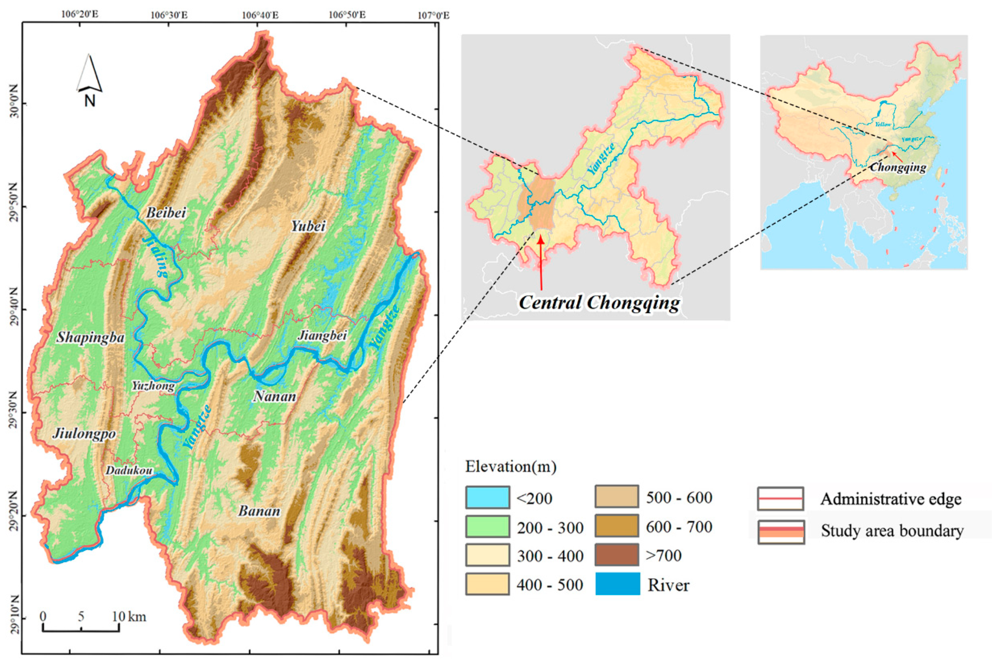
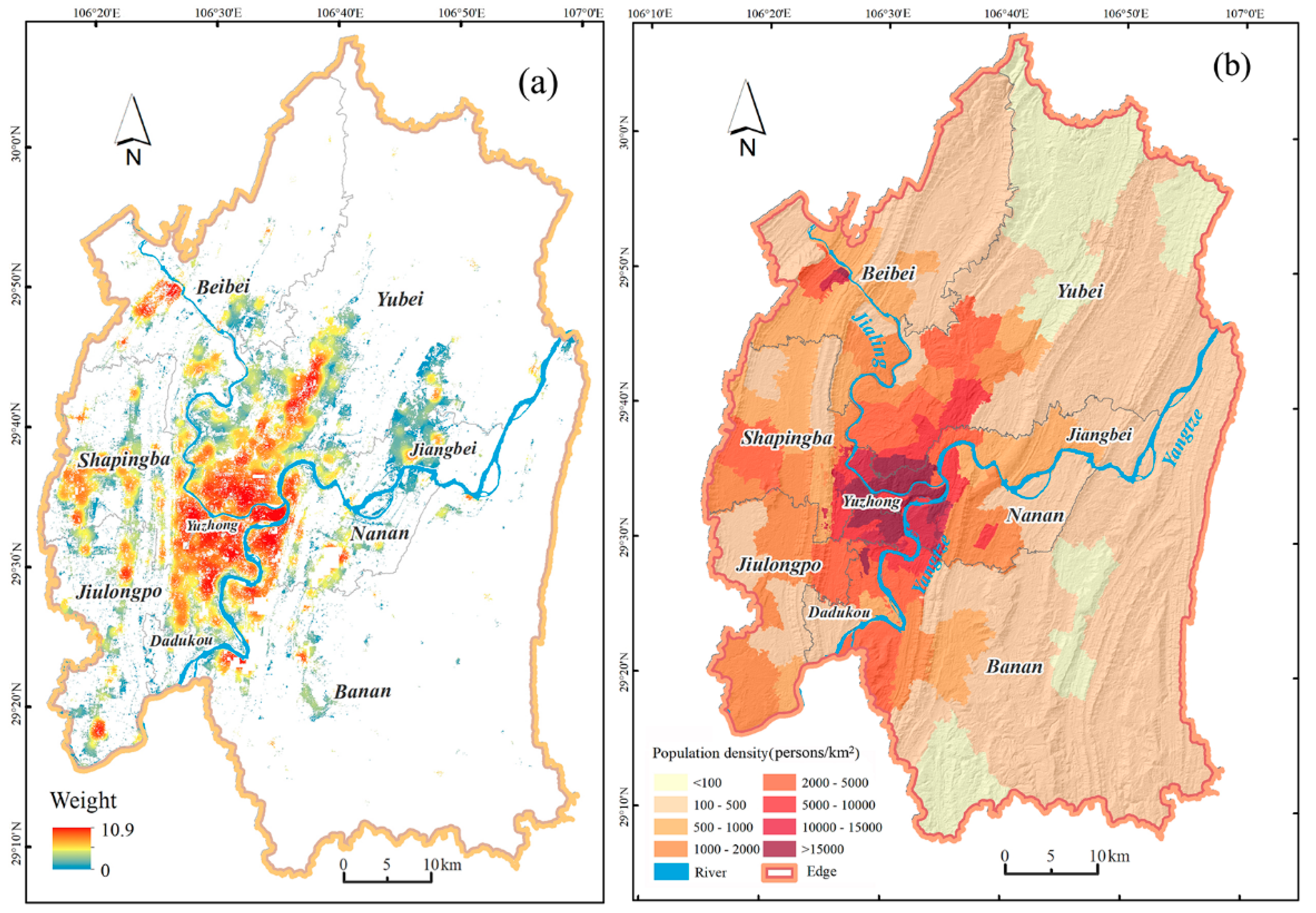
2.1. Study Area
2.2. Datasets
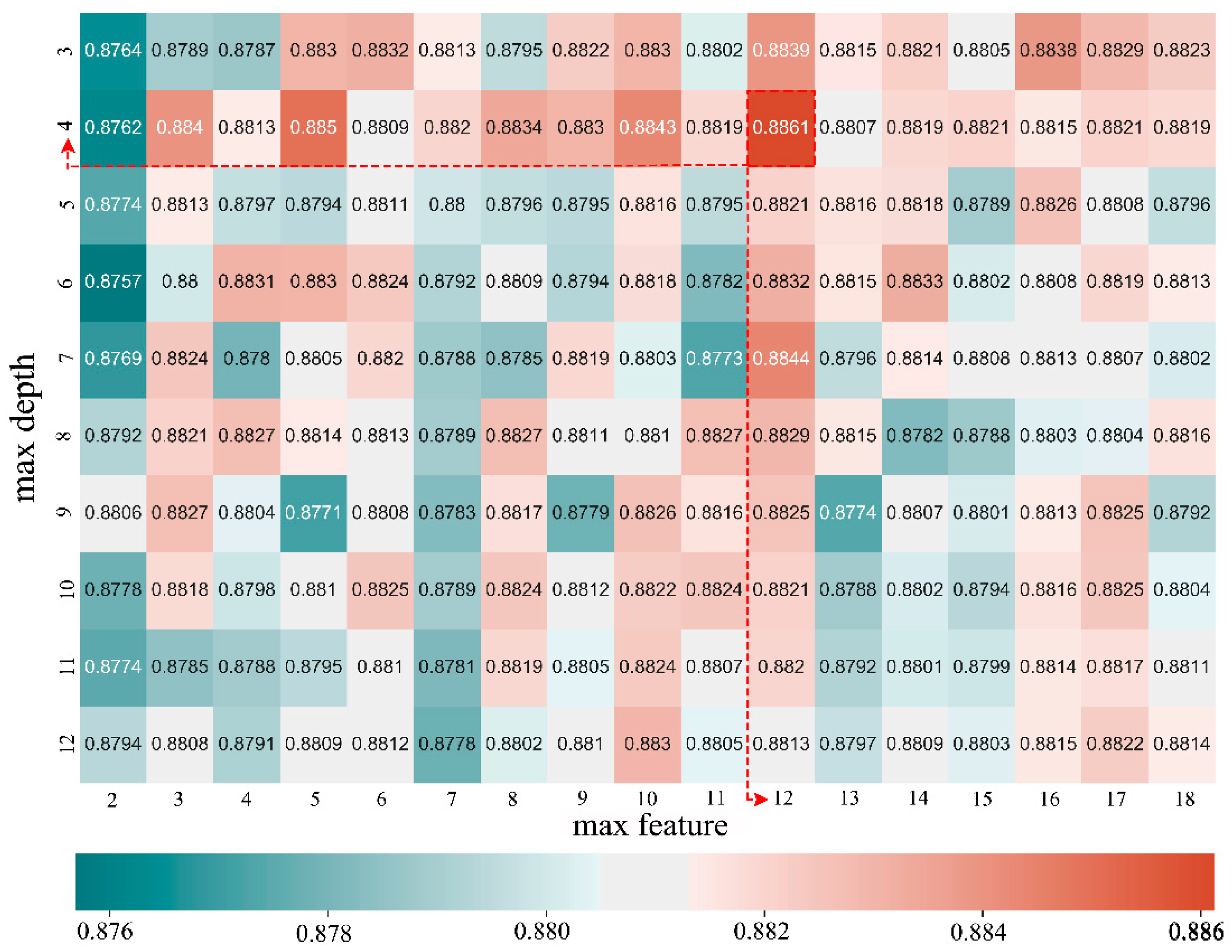
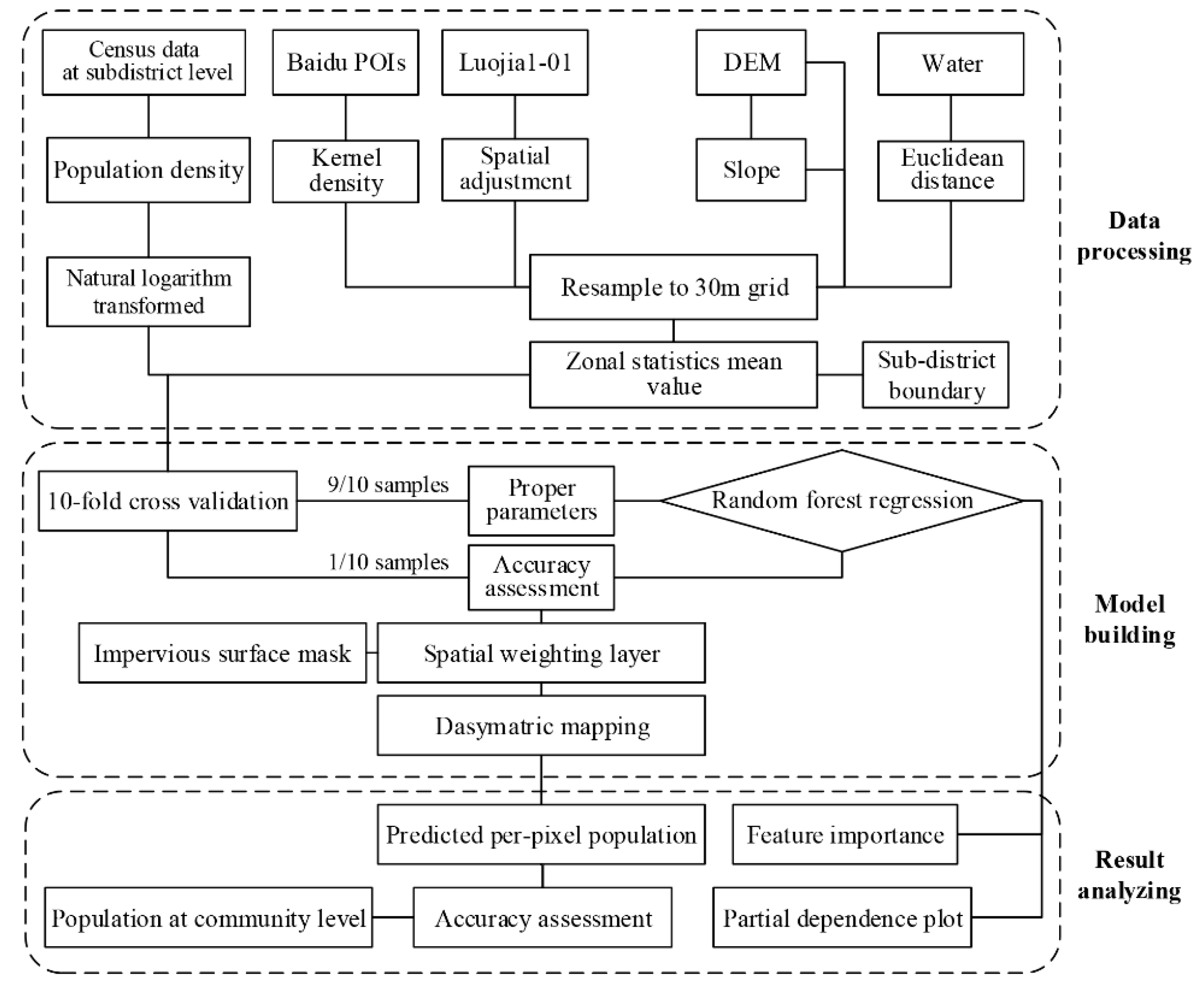
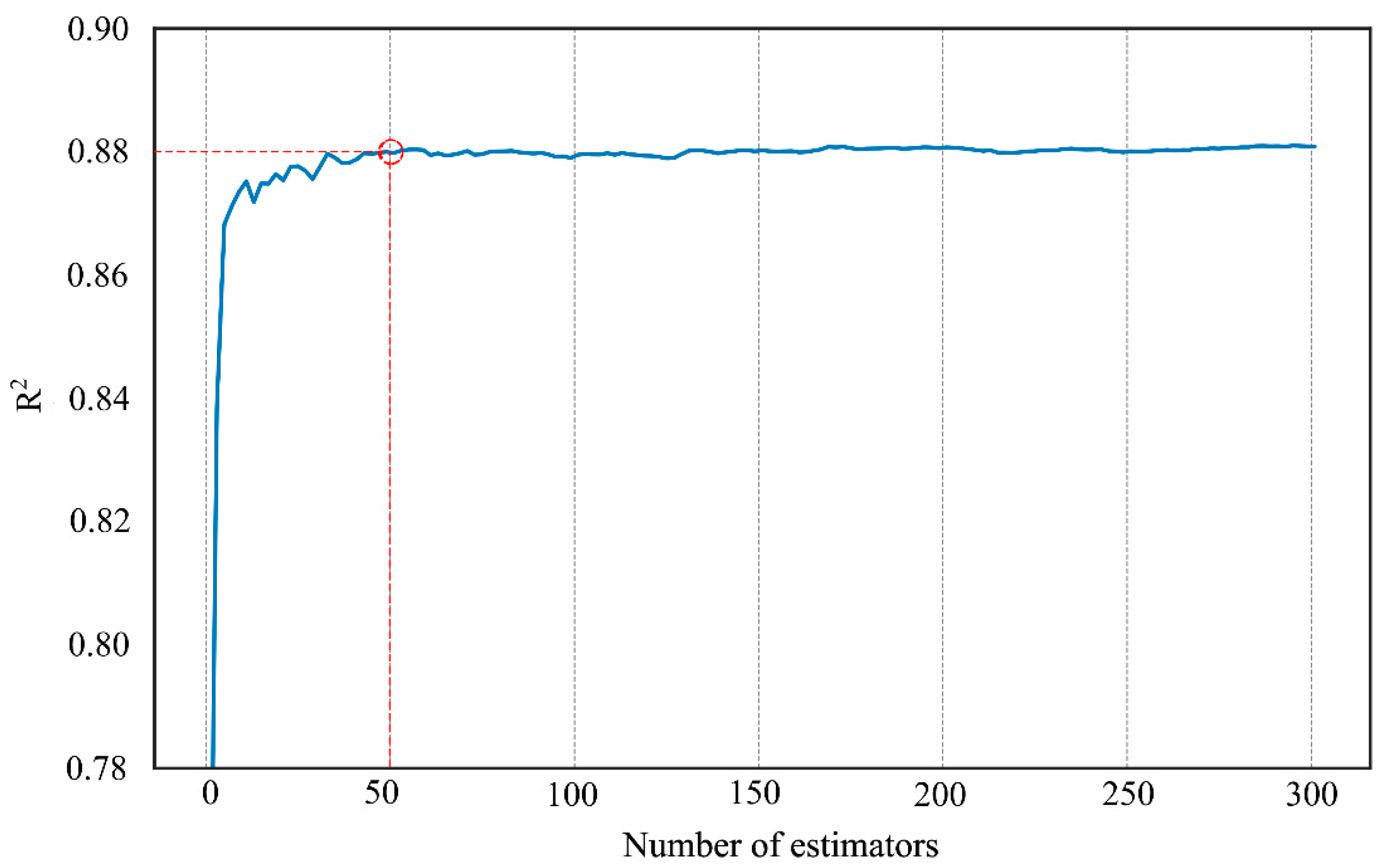
2.3. Methods
3. Results
3.1. Population Estimation
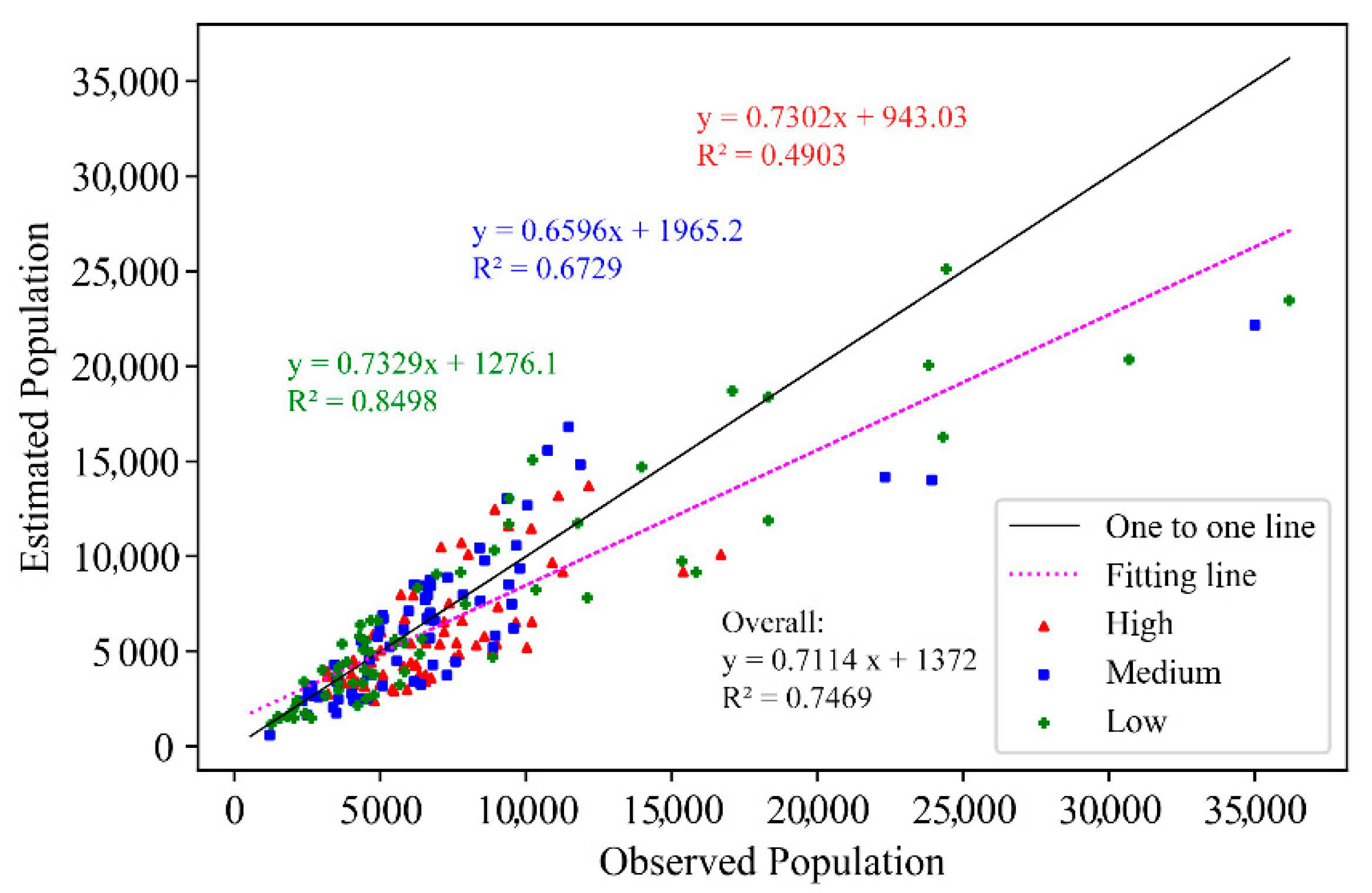
3.2. Accuracy Validation
4. Discussion
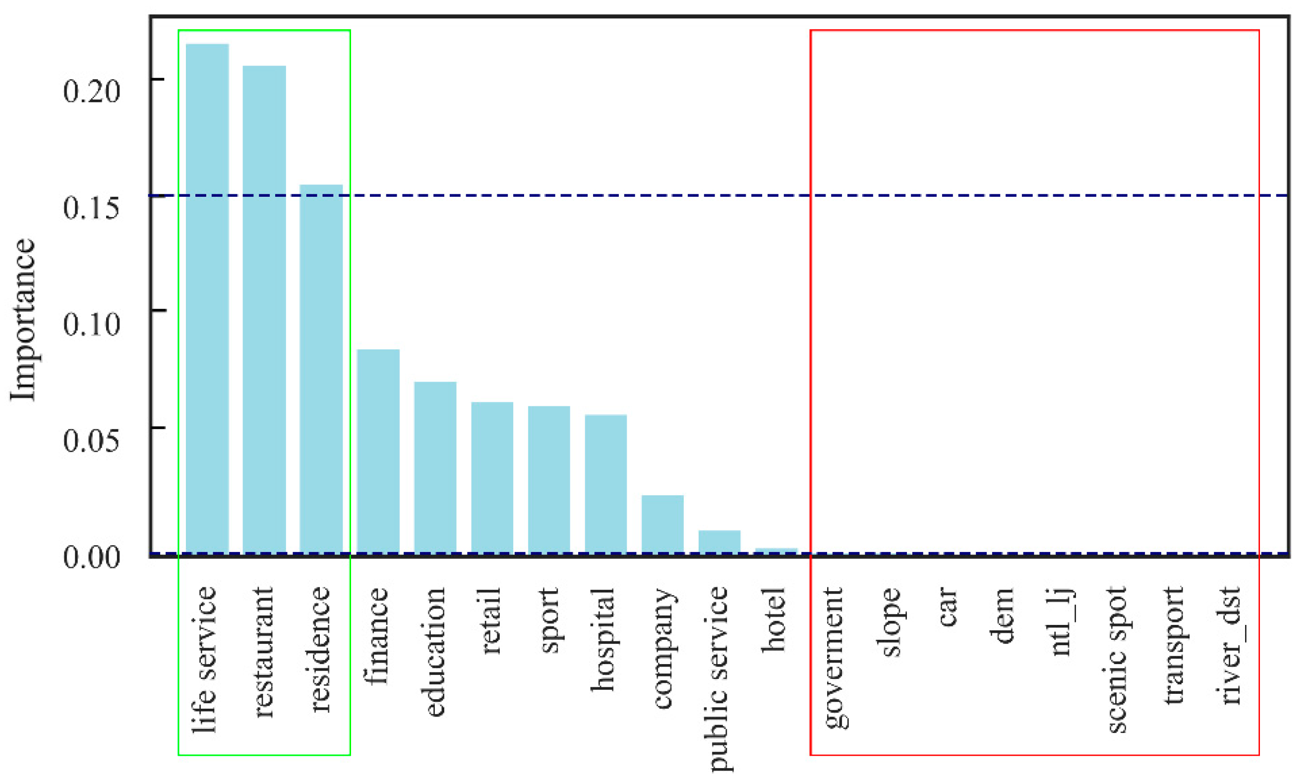
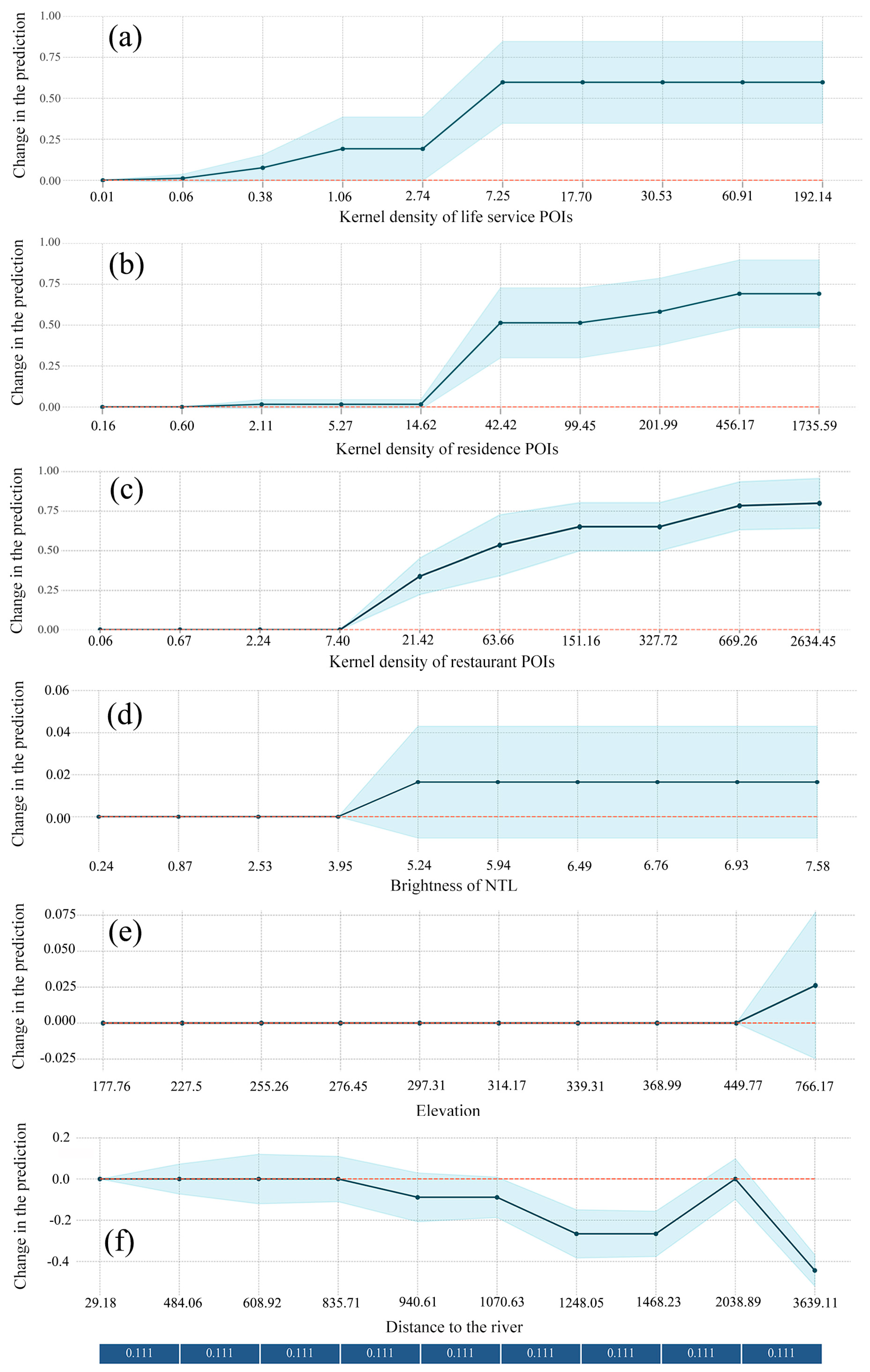
4.1. Interpretation of the Gridded Population
4.2. Principal Findings and Meaningful Implication
4.3. Limitations and Future Research
5. Conclusions
Author Contributions
Funding
Acknowledgments
Conflicts of Interest
References
- Azar, D.; Engstrom, R.; Graesser, J.; Comenetz, J. Generation of fine-scale population layers using multi-resolution satellite imagery and geospatial data. Remote Sens. Environ. 2013, 130, 219–232. [Google Scholar] [CrossRef]
- Balk, D.; Deichmann, U.; Yetman, G.; Pozzi, F.; Hay, S.I.; Nelson, A. Determining global population distribution: Methods, applications and data. Adv. Parasitol. 2006, 62, 119–156. [Google Scholar] [CrossRef] [PubMed] [Green Version]
- Weber, E.; Seaman, V.Y.; Stewart, R.; Bird, T.J.; Tatem, A.J.; McKee, J.; Bhaduri, B.; Moehl, J.J.; Reith, A.E. Census-independent population mapping in northern Nigeria. Remote Sens. Environ. 2018, 204, 786–798. [Google Scholar] [CrossRef] [PubMed]
- O’Neill, B.C.C.; Dalton, M.; Fuchs, R.; Jiang, L.; Pachauri, S.; Zigova, K. Global demographic trends and future carbon emissions. Proc. Natl. Acad. Sci. USA 2010, 107, 17521–17526. [Google Scholar] [CrossRef] [PubMed] [Green Version]
- Gaughan, A.E.; Stevens, F.R.; Linard, C.; Jia, P.; Tatem, A.J. High Resolution Population Distribution Maps for Southeast Asia in 2010 and 2015. PLoS ONE 2013, 8, e55882. [Google Scholar] [CrossRef]
- Su, H.; Wei, H.; Zhao, J. Density effect and optimum density of the urban population in China. Urban Stud. 2016, 54, 1760–1777. [Google Scholar] [CrossRef]
- Deville, P.; Linard, C.; Martin, S.; Gilbert, M.; Stevens, F.R.; Gaughan, A.E.; Blondel, V.D.; Tatem, A.J. Dynamic population mapping using mobile phone data. Proc. Natl. Acad. Sci. USA 2014, 111, 15888–15893. [Google Scholar] [CrossRef] [Green Version]
- Yao, Y.; Liu, X.; Li, X.; Zhang, J.; Liang, Z.; Mai, K.; Zhang, Y. Mapping fine-scale population distributions at the building level by integrating multisource geospatial big data. Int. J. Geogr. Inf. Sci. 2017, 31, 1220–1244. [Google Scholar] [CrossRef]
- Bakillah, M.; Liang, S.; Mobasheri, A.; Arsanjani, J.J.; Zipf, A. Fine-resolution population mapping using OpenStreetMap points-of-interest. Int. J. Geogr. Inf. Sci. 2014, 28, 1940–1963. [Google Scholar] [CrossRef]
- Wardrop, N.A.; Jochem, W.C.; Bird, T.J.; Chamberlain, H.R.; Clarke, D.; Kerr, D.; Bengtsson, L.; Juran, S.; Seaman, V.; Tatem, A.J. Spatially disaggregated population estimates in the absence of national population and housing census data. Proc. Natl. Acad. Sci. USA 2018, 115, 3529–3537. [Google Scholar] [CrossRef] [Green Version]
- Goodchild, M.F.; Anselin, L.; Deichmann, U. A framework for the areal interpolation of socioeconomic data. Environ. Plan A Econ. Space 1993, 25, 383–397. [Google Scholar] [CrossRef]
- Doxsey-Whitfield, E.; MacManus, K.; Adamo, S.B.; Pistolesi, L.; Squires, J.; Borkovska, O.; Baptista, S.R. Taking Advantage of the Improved Availability of Census Data: A First Look at the Gridded Population of the World, Version 4. Pap. Appl. Geogr. 2015, 1, 226–234. [Google Scholar] [CrossRef]
- Tobler, W.; Deichmann, U.; Gottsegen, J.; Maloy, K. World Population in a Grid of Spherical Quadrilaterals. Int. J. Popul. Geogr. 1997, 3, 203–225. [Google Scholar] [CrossRef]
- Dobson, J.E.; Brlght, E.A.; Coleman, P.R.; Durfee, R.C.; Worley, B.A. LandScan:A Global Population Database for Estimating Populations at Risk. Photogramm. Eng. Remote Sens. 2000, 66, 849–857. [Google Scholar]
- Tatem, A.J. Comment: WorldPop, open data for spatial demography. Sci. Data 2017, 4, 170004. [Google Scholar] [CrossRef]
- Reed, F.J.; Gaughan, A.E.; Stevens, F.R.; Yetman, G.; Sorichetta, A.; Tatem, A.J. Gridded Population Maps Informed by Different Built Settlement Products. Data 2018, 3, 33. [Google Scholar] [CrossRef] [Green Version]
- Ye, T.; Zhao, N.; Yang, X.; Ouyang, Z.; Liu, X.; Chen, Q.; Hu, K.; Yue, W.; Qi, J.; Li, Z.; et al. Improved population mapping for China using remotely sensed and points-of-interest data within a random forests model. Sci. Total Environ. 2019, 658, 936–946. [Google Scholar] [CrossRef]
- Jia, P.; Qiu, Y.; Gaughan, A.E. A fine-scale spatial population distribution on the High-resolution Gridded Population Surface and application in Alachua County, Florida. Appl. Geogr. 2014, 50, 99–107. [Google Scholar] [CrossRef]
- Wang, L.; Fan, H.; Wang, Y. Fine-Resolution Population Mapping from International Space Station Nighttime Photography and Multisource Social Sensing Data Based on Similarity Matching. Remote Sens. 2019, 11, 1900. [Google Scholar] [CrossRef] [Green Version]
- Stevens, F.R.; Gaughan, A.E.; Linard, C.; Tatem, A.J. Disaggregating census data for population mapping using random forests with remotely-sensed and ancillary data. PLoS ONE 2015, 10, e0107042. [Google Scholar] [CrossRef] [Green Version]
- Gao, N.; Li, F.; Zeng, H.; Van Bilsen, D.; De Jong, M. Can More Accurate Night-Time Remote Sensing Data Simulate a More Detailed Population Distribution? Sustainability 2019, 11, 4488. [Google Scholar] [CrossRef] [Green Version]
- Mossoux, S.; Kervyn, M.; Soulé, H.; Canters, F. Mapping Population Distribution from High Resolution Remotely Sensed Imagery in a Data Poor Setting. Remote Sens. 2018, 10, 1409. [Google Scholar] [CrossRef] [Green Version]
- Zeng, C.; Zhou, Y.; Wang, S.; Yan, F.; Zhao, Q. Population spatialization in China based on night-time imagery and land use data. Int. J. Remote Sens. 2011, 32, 9599–9620. [Google Scholar] [CrossRef]
- Yu, B.; Lian, T.; Huang, Y.; Yao, S.; Ye, X.; Chen, Z.; Yang, C.; Wu, J. Integration of nighttime light remote sensing images and taxi GPS tracking data for population surface enhancement. Int. J. Geogr. Inf. Sci. 2019, 33, 687–706. [Google Scholar] [CrossRef]
- Langford, M. An Evaluation of Small Area Population Estimation Techniques Using Open Access Ancillary Data. Geogr. Anal. 2013, 45, 324–344. [Google Scholar] [CrossRef]
- Yang, X.; Ye, T.; Zhao, N.; Chen, Q.; Yue, W.; Qi, J.; Zeng, B.; Jia, P. Population Mapping with Multisensor Remote Sensing Images and Point-Of-Interest Data. Remote Sens. 2019, 11, 574. [Google Scholar] [CrossRef] [Green Version]
- Liu, Y.; Liu, X.; Gao, S.; Gong, L.; Kang, C.; Zhi, Y.; Chi, G.; Shi, L. Social Sensing: A New Approach to Understanding Our Socioeconomic Environments. Ann. Assoc. Am. Geogr. 2015, 105, 512–530. [Google Scholar] [CrossRef]
- Lin, J.; Cromley, R.G. Evaluating geo-located Twitter data as a control layer for areal interpolation of population. Appl. Geogr. 2015, 58, 41–47. [Google Scholar] [CrossRef]
- Shi, X.; Li, M.; Hunter, O.; Guetti, B.; Andrew, A.; Stommel, E.; Bradley, W.; Karagas, M.R. Estimation of environmental exposure: Interpolation, kernel density estimation or snapshotting. Ann. GIS 2019, 25, 1–8. [Google Scholar] [CrossRef] [Green Version]
- Qiu, F.; Cromley, R. Areal Interpolation and Dasymetric Modeling. Geogr. Anal. 2013, 45, 213–215. [Google Scholar] [CrossRef]
- Azar, D.; Graesser, J.; Engstrom, R.; Comenetz, J.; Leddy, R.M.; Schechtman, N.G.; Andrews, T. Spatial refinement of census population distribution using remotely sensed estimates of impervious surfaces in Haiti. Int. J. Remote Sens. 2010, 31, 5635–5655. [Google Scholar] [CrossRef]
- Li, J.; Li, J.; Yuan, Y.; Li, G. Spatiotemporal distribution characteristics and mechanism analysis of urban population density: A case of Xi’an, Shaanxi, China. Cities 2019, 86, 62–70. [Google Scholar] [CrossRef]
- Liu, Y.; Fan, P.; Yue, W.; Song, Y. Impacts of land finance on urban sprawl in China: The case of Chongqing. Land Use Policy 2018, 72, 420–432. [Google Scholar] [CrossRef]
- Bao, H.X.H.; Li, L.; Lizieri, C. City profile: Chongqing (1997–2017). Cities 2019, 94, 161–171. [Google Scholar] [CrossRef]
- Cheng, L.; Guan, D.; Zhou, L.; Zhao, Z.; Zhou, J. Urban cooling island effect of main river on a landscape scale in Chongqing, China. Sustain. Cities Soc. 2019, 47, 101501. [Google Scholar] [CrossRef]
- Chen, S.; Yan, Y.; Liu, G.; Fang, D.; Wu, Z.; He, J.; Tang, J. Spatiotemporal characteristics of precipitation diurnal variations in Chongqing with complex terrain. Theor. Appl. Clim. 2018, 137, 1217–1231. [Google Scholar] [CrossRef]
- Silverman, B.W. Kernel Density Estimation Using the Fast Fourier Transform. Appl. Stat. 1982, 31, 93. [Google Scholar] [CrossRef]
- Jiang, W.; He, G.; Long, T.; Guo, H.; Yin, R.; Leng, W.; Liu, H.; Wang, G. Potentiality of Using Luojia 1-01 Nighttime Light Imagery to Investigate Artificial Light Pollution. Sensors 2018, 18, 2900. [Google Scholar] [CrossRef] [Green Version]
- Ou, J.; Liu, X.; Liu, P.; Liu, X. Evaluation of Luojia 1-01 nighttime light imagery for impervious surface detection: A comparison with NPP-VIIRS nighttime light data. Int. J. Appl. Earth Obs. Geoinf. 2019, 81, 1–12. [Google Scholar] [CrossRef]
- Wang, C.; Chen, Z.; Yang, C.; Li, Q.; Wu, Q.; Wu, J.; Zhang, G.; Yu, B. Analyzing parcel-level relationships between Luojia 1-01 nighttime light intensity and artificial surface features across Shanghai, China: A comparison with NPP-VIIRS data. Int. J. Appl. Earth Obs. Geoinf. 2020, 85, 101989. [Google Scholar] [CrossRef]
- Breiman, L.E.O. Random Forests. Mach. Learn. 2001, 45, 5–32. [Google Scholar] [CrossRef] [Green Version]
- Biau, G.; Scornet, E. A random forest guided tour. Test 2016, 25, 197–227. [Google Scholar] [CrossRef] [Green Version]
- Robinson, R.L.M.; Palczewska, A.; Palczewski, J.; Kidley, N. Comparison of the Predictive Performance and Interpretability of Random Forest and Linear Models on Benchmark Data Sets. J. Chem. Inf. Model. 2017, 57, 1773–1792. [Google Scholar] [CrossRef] [PubMed]
- Criminisi, A.; Shotton, J.; Konukoglu, E. Decision forests: A unified framework for classification, regression, density estimation, manifold learning and semi-supervised learning. Found. Trends Comput. Graph. Vis. 2011, 7, 81–227. [Google Scholar] [CrossRef]
- Boulesteix, A.-L.; Janitza, S.; Kruppa, J.; König, I.R. Overview of random forest methodology and practical guidance with emphasis on computational biology and bioinformatics. Wiley Interdiscip. Rev. Data Min. Knowl. Discov. 2012, 2, 493–507. [Google Scholar] [CrossRef] [Green Version]
- Oh, Y.J.; Park, H.S.; Min, Y. Understanding location-based service application connectedness: Model development and cross-validation. Comput. Hum. Behav. 2019, 94, 82–91. [Google Scholar] [CrossRef]
- Gholinejad, S.; Naeini, A.A.; Amiri-Simkooei, A.R. Robust Particle Swarm Optimization of RFMs for High-Resolution Satellite Images Based on K-Fold Cross-Validation. IEEE J. Sel. Top. Appl. Earth Obs. Remote. Sens. 2019, 12, 2594–2599. [Google Scholar] [CrossRef]
- Brunsdon, C.; Fotheringham, A.S.; Charlton, M.E. Geographically Weighted Regression: A Method for Exploring Spatial Nonstationarity. Geogr. Anal. 1996, 28, 281–298. [Google Scholar] [CrossRef]
- Brunsdon, C.; Fotheringham, S.; Charlton, M. Geographically Weighted Regression. J. R. Stat. Soc. Ser. D (Stat.) 1998, 47, 431–443. [Google Scholar] [CrossRef]
- McMillen, D.P. Geographically Weighted Regression: The Analysis of Spatially Varying Relationships. Am. J. Agric. Econ. 2004, 86, 554–556. [Google Scholar] [CrossRef]
- Matthews, S.A.; Yang, T.-C. Mapping the results of local statistics: Using geographycally weigthed regresion. Demogr. Res. 2012, 26, 151–166. [Google Scholar] [CrossRef] [PubMed] [Green Version]
- Benassi, F.; Naccarato, A. Households in potential economic distress. A geographically weighted regression model for Italy, 2001–2011. Spat. Stat. 2017, 21, 362–376. [Google Scholar] [CrossRef]
- Akaike, H. A new look at the statistical model identification. IEEE Trans. Autom. Control. 1974, 19, 716–723. [Google Scholar] [CrossRef]
- Oshan, T.M.; Li, Z.; Kang, W.; Wolf, L.J.; Fotheringham, A.S. MGWR: A Python Implementation of Multiscale Geographically Weighted Regression for Investigating Process Spatial Heterogeneity and Scale. ISPRS Int. J. Geo Inf. 2019, 8, 269. [Google Scholar] [CrossRef] [Green Version]
- Burnham, K.P.; Anderson, D.R. Multimodel inference: Understanding AIC and BIC in Model Selection. Sociol. Methods Res. 2004, 33, 261–304. [Google Scholar] [CrossRef]
- Friedman, J.H. Greedy function approximation: A gradient boosting machine. Ann. Stat. 2001, 29, 1189–1232. [Google Scholar] [CrossRef]
- Grömping, U. Variable Importance Assessment in Regression: Linear Regression versus Random Forest. Am. Stat. 2009, 63, 308–319. [Google Scholar] [CrossRef]
- Gregorutti, B.; Michel, B.; Saint-Pierre, P. Correlation and variable importance in random forests. Stat. Comput. 2017, 27, 659–678. [Google Scholar] [CrossRef] [Green Version]
- Zhao, Q.; Hastie, T. Causal Interpretations of Black-Box Models. J. Bus. Econ. Stat. 2019, 1–10. [Google Scholar] [CrossRef]
- Linard, C.; Alegana, V.A.; Noor, A.; Snow, R.W.; Tatem, A.J. A high resolution spatial population database of Somalia for disease risk mapping. Int. J. Health Geogr. 2010, 9, 45. [Google Scholar] [CrossRef]
- Yang, H. China must continue the momentum of green law. Nature 2014, 509, 535. [Google Scholar] [CrossRef] [PubMed] [Green Version]
- Amaral, S.; Monteiro, A.M.V.; Camara, G.; Quintanilha, J.A. DMSP/OLS night-time light imagery for urban population estimates in the Brazilian Amazon. Int. J. Remote Sens. 2006, 27, 855–870. [Google Scholar] [CrossRef]
- Townsend, A.C.; Bruce, D. The use of night-time lights satellite imagery as a measure of Australia’s regional electricity consumption and population distribution. Int. J. Remote Sens. 2010, 31, 4459–4480. [Google Scholar] [CrossRef]
- Li, X.; Zhou, W. Dasymetric mapping of urban population in China based on radiance corrected DMSP-OLS nighttime light and land cover data. Sci. Total. Environ. 2018, 643, 1248–1256. [Google Scholar] [CrossRef]
- Jiang, S.; Alves, A.; Rodrigues, F.; Ferreira, J.; Pereira, F.C. Mining point-of-interest data from social networks for urban land use classification and disaggregation. Comput. Environ. Urban Syst. 2015, 53, 36–46. [Google Scholar] [CrossRef] [Green Version]
- Hu, T.; Yang, J.; Li, X.; Gong, P. Mapping Urban Land Use by Using Landsat Images and Open Social Data. Remote Sens. 2016, 8, 151. [Google Scholar] [CrossRef]
- Arsanjani, J.J.; Helbich, M.; Bakillah, M.; Hagenauer, J.; Zipf, A. Toward mapping land-use patterns from volunteered geographic information. Int. J. Geogr. Inf. Sci. 2013, 27, 2264–2278. [Google Scholar] [CrossRef]
- Ma, D.; Sandberg, M.; Jiang, B. Characterizing the Heterogeneity of the OpenStreetMap Data and Community. ISPRS Int. J. Geo Inf. 2015, 4, 535–550. [Google Scholar] [CrossRef]


| Dataset | Scope | Resolution | Method | Ancillary Data |
|---|---|---|---|---|
| GPWv4 | World | 1 km | Areal-weighting | Land cover dataset |
| GRUMP | World | 1 km | Mass-conserving | Night–time lights dataset and buffered settlement centroids |
| LandScan | World | 1 km | Smart interpolation | Roads, slope, land cover, Night–time lights, etc. |
| Worldpop | World | 100 m | Random forest | Settlement location and extent, land cover, satellite nightlights, topography, roads, buildings, etc. |
| Our research | Complex city | 30 m | Random forest | Points of interest, satellite nighttime lights, topography, etc. |
| Dataset | Format | Time | Source |
|---|---|---|---|
| Census data at the subdistrict and community levels | Table | 2018 | Chongqing Bureau of Public Security, China |
| Administrative Boundary | Vector (polygon) | 2018 | Chongqing Planning and Design Institute, China |
| Points of interest | Vector (point) | 2018 | Baidu, Inc., China |
| Luojia1-01 images | Raster (130 m) | 2018 | Wuhan University, China |
| Water | Vector (polygon) | 2018 | Chongqing Planning and Design Institute, China |
| Impervious surface | Vector (polygon) | 2018 | Chongqing Planning and Design Institute, China |
| ASTER GDEM | Raster (30 m) | 2010 | American NASA Jet Propulsion Lab and Japan’s Ministry of Economy, Trade and Industry |
| Category | Quantity | Percentage | Examples |
|---|---|---|---|
| Car | 24,350 | 3.22% | Garage, car lot |
| Company | 67,930 | 8.99% | Enterprise, factory |
| Education | 28,622 | 3.79% | School, training agency |
| Finance | 11,681 | 1.55% | Bank, insurance company |
| Government | 16,816 | 2.22% | Police station, weather bureau |
| Hospital | 25,871 | 3.42% | Pharmacy, clinic |
| Hotel | 21,182 | 2.80% | Inn, lodge |
| Life service | 123,309 | 16.31% | Post office, laundry |
| Public service | 7081 | 0.94% | Newsstands, washroom |
| Residence | 18,513 | 2.45% | Apartment, house |
| Restaurant | 183,273 | 24.24% | Hotpot restaurant, tea house |
| Retail | 203,418 | 26.91% | Supermarket, shopping center |
| Scenic spot | 3459 | 0.46% | Monument, forest park |
| Sport | 20,506 | 2.71% | Stadium, gymnasium |
| Methodology | Akaike Criterion | Validation R2 | RMSE | MAE |
|---|---|---|---|---|
| MLR | 366.78 | 0.7199 | 2944.25 | 2056.81 |
| GWR | 357.29 | 0.7221 | 2939.09 | 2042.35 |
| RFR | – | 0.7469 | 2785.04 | 1889.70 |
© 2020 by the authors. Licensee MDPI, Basel, Switzerland. This article is an open access article distributed under the terms and conditions of the Creative Commons Attribution (CC BY) license (http://creativecommons.org/licenses/by/4.0/).
Share and Cite
Zhou, Y.; Ma, M.; Shi, K.; Peng, Z. Estimating and Interpreting Fine-Scale Gridded Population Using Random Forest Regression and Multisource Data. ISPRS Int. J. Geo-Inf. 2020, 9, 369. https://0-doi-org.brum.beds.ac.uk/10.3390/ijgi9060369
Zhou Y, Ma M, Shi K, Peng Z. Estimating and Interpreting Fine-Scale Gridded Population Using Random Forest Regression and Multisource Data. ISPRS International Journal of Geo-Information. 2020; 9(6):369. https://0-doi-org.brum.beds.ac.uk/10.3390/ijgi9060369
Chicago/Turabian StyleZhou, Yun, Mingguo Ma, Kaifang Shi, and Zhenyu Peng. 2020. "Estimating and Interpreting Fine-Scale Gridded Population Using Random Forest Regression and Multisource Data" ISPRS International Journal of Geo-Information 9, no. 6: 369. https://0-doi-org.brum.beds.ac.uk/10.3390/ijgi9060369