Uncorrelated Geo-Text Inhibition Method Based on Voronoi K-Order and Spatial Correlations in Web Maps

Abstract
:
1. Introduction
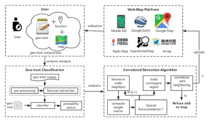
2. Uncorrelated Geo-Text Detection Method
2.1. Automatic Classification for Geo-Text Annotations
2.1.1. Geo-Texts Types
2.1.2. Automatic Classification Method
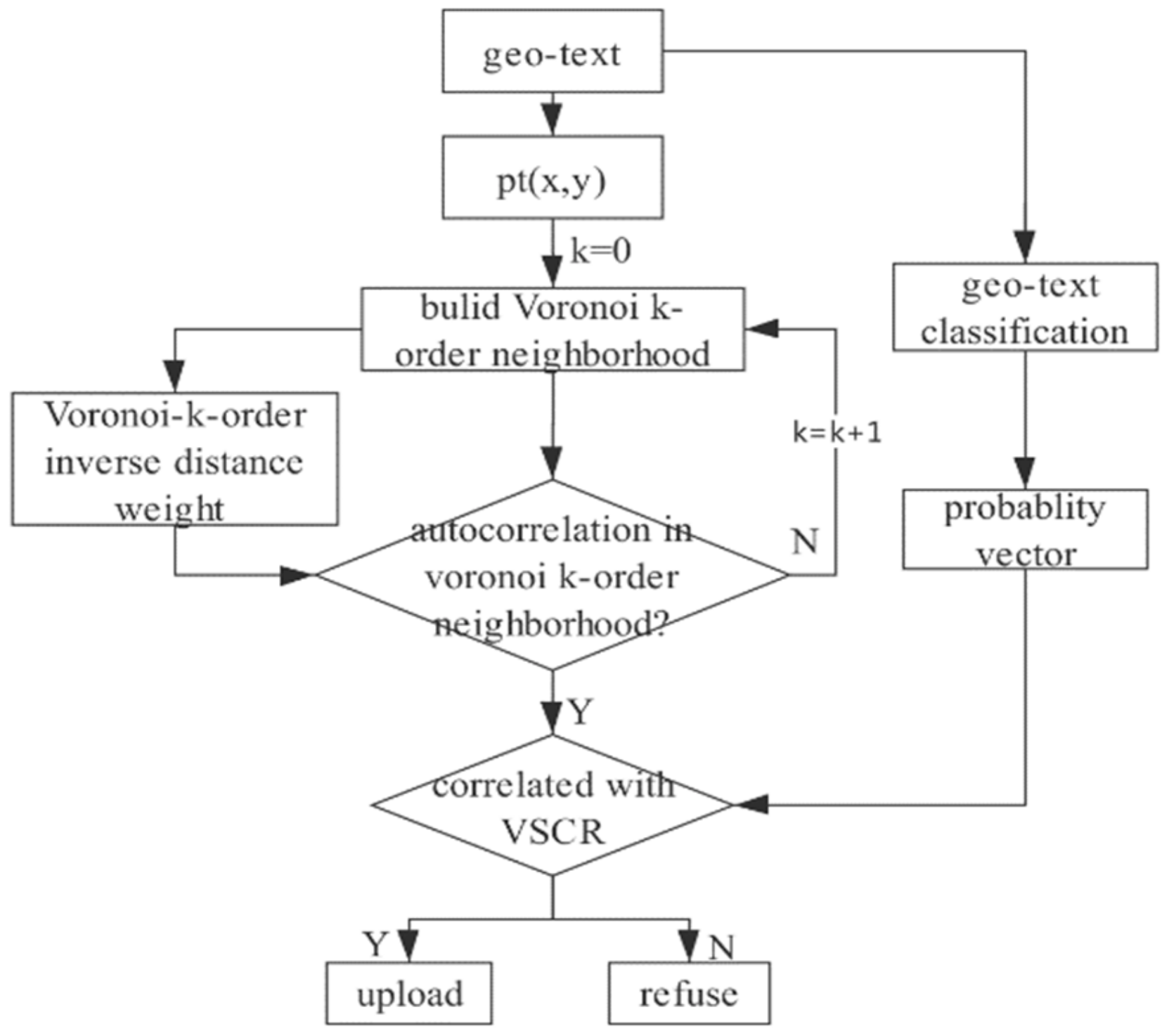
2.2. Correlated Geo-Text Detection Algorithm (CGD)
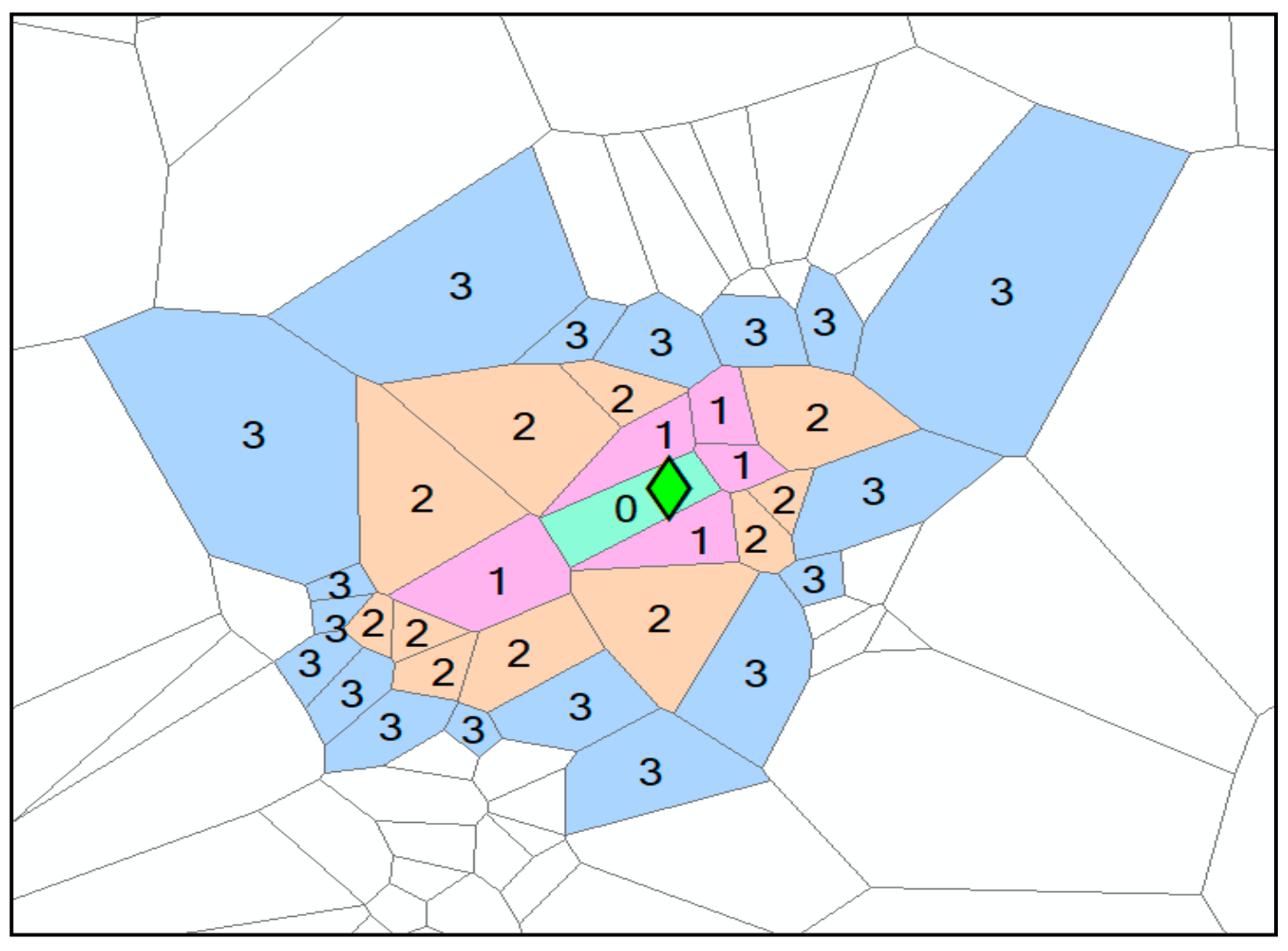
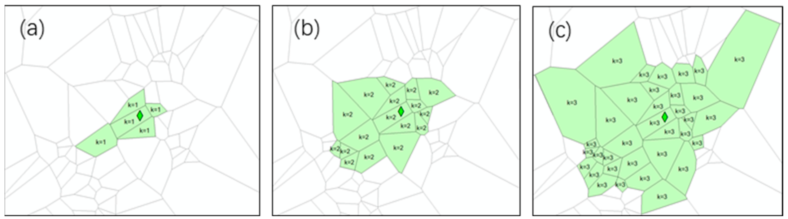
2.2.1. Voronoi k-Order Neighborhood Partition
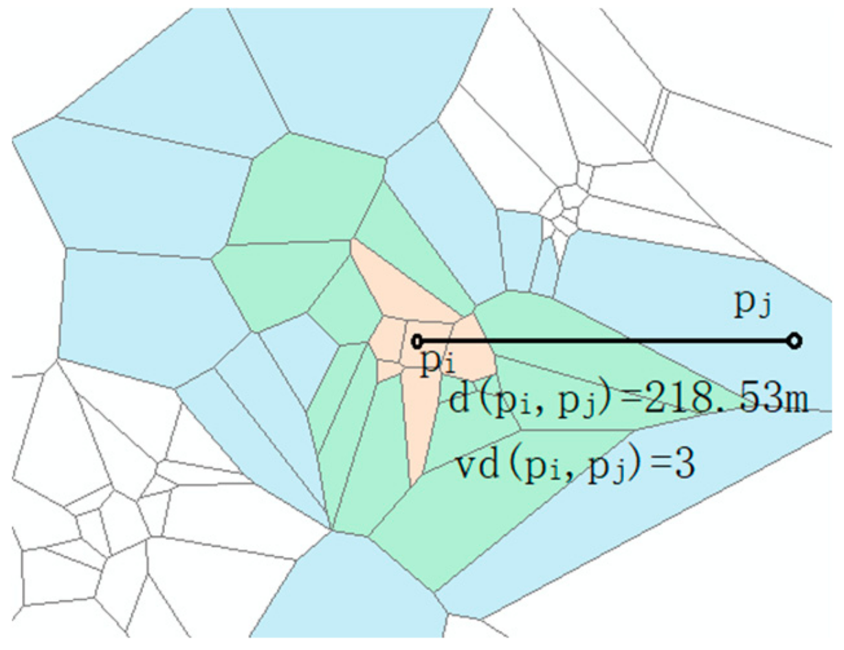
2.2.2. Weight Matrix Based on Voronoi k-Order Neighborhood
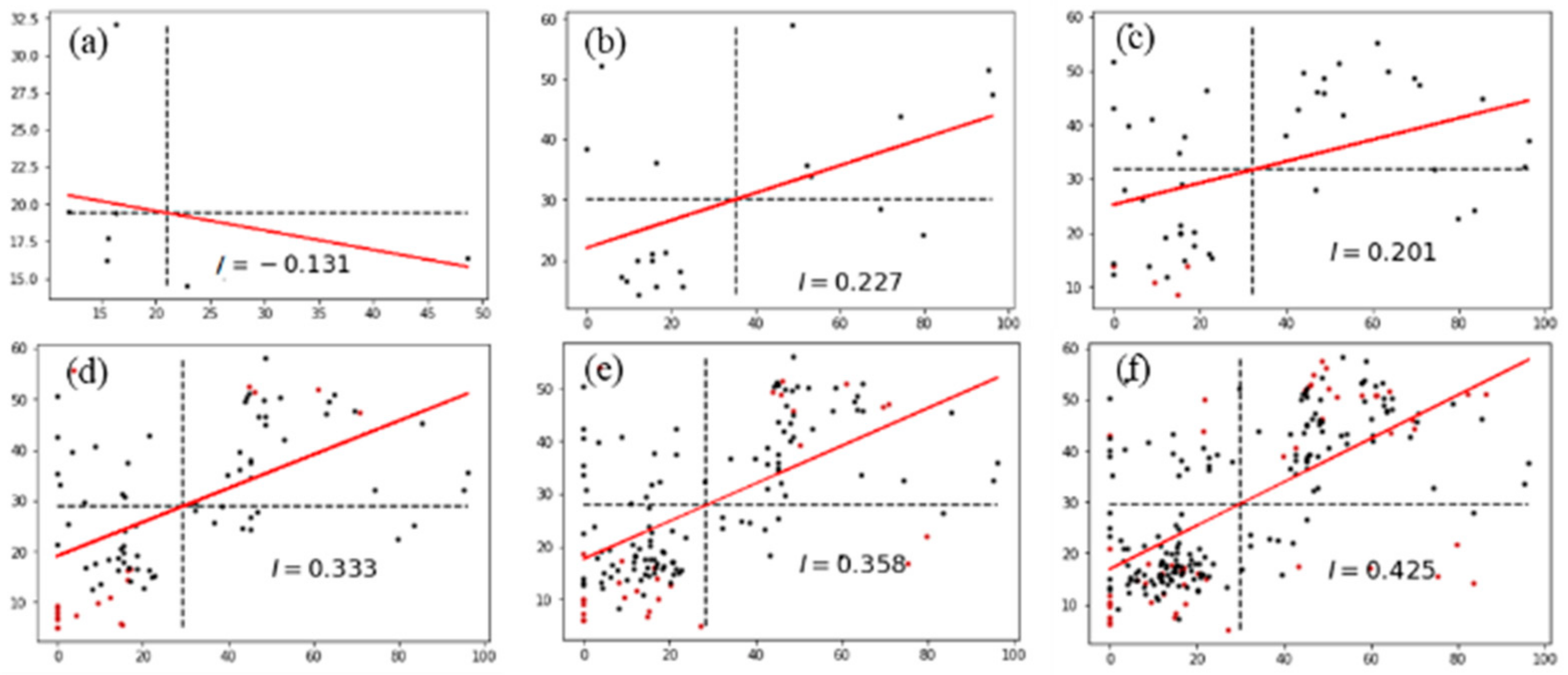
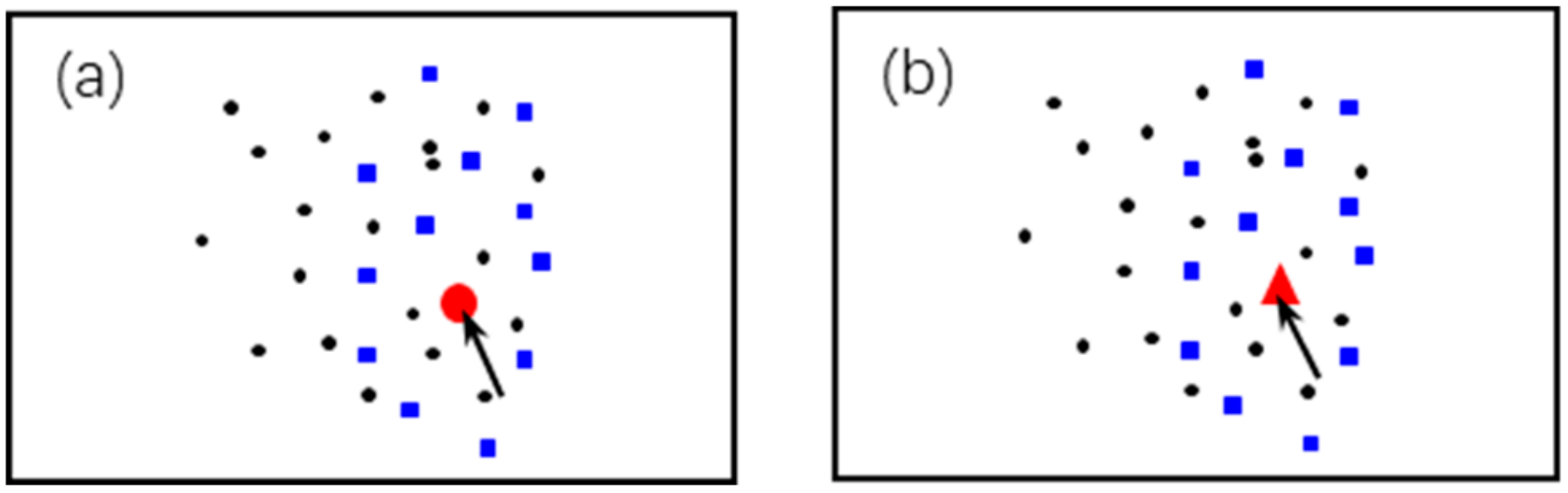
2.2.3. Detecting the Minimum Voronoi-k-Order Semantic Convergence Region of A Point
2.2.4. Similarity Analysis of Geo-Text Annotation in VSCR
3. Experiment Validation
3.1. Auto Classification of Geo-Texts
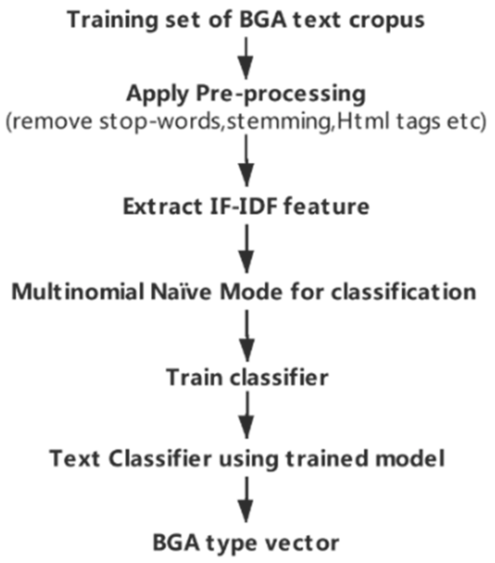
3.1.1. Train Classifier
3.1.2. Geo-Text Classification Process
3.2. Correlated Geo-Text Detection (CGD) Algorithm Experiment
3.2.1. CGD Algorithm Process
3.2.2. Variant Phenomenon Detection
3.3. Experimental Results Analysis
3.3.1. Geo-Text Classification Results
3.3.2. Result of CGD Algorithm
4. Discussion
5. Conclusions
Author Contributions
Funding
Acknowledgments
Conflicts of Interest
References
- Cardone, G.; Cirri, A.; Corradi, A.; Foschini, L. The ParticipAct Mobile Crowd Sensing Living Lab: The Testbed for Smart Cities. IEEE Commun. Mag. 2014, 52, 78–85. [Google Scholar] [CrossRef]
- Du, H.; Anand, S.; Alechina, N.; Morley, J.; Hart, G.; Leibovici, D.; Jackson, M.; Ware, M. Geospatial Information Integration for Authoritative and Crowd Sourced Road Vector Data. Trans. GIS 2012, 16, 455–476. [Google Scholar] [CrossRef]
- Du, H.; Alechina, N.; Jackson, M.; Hart, G. A Method for Matching Crowd-sourced and Authoritative Geospatial Data. Trans. GIS 2017, 21, 406–427. [Google Scholar] [CrossRef] [Green Version]
- Zhang, Y. Pattern-mining approach for conflating crowdsourcing road networks with POIs. Int. J. Geogr. Inf. Sci. 2015, 29, 786–805. [Google Scholar] [CrossRef]
- Lyu, H.; Sheng, Y.; Guo, N.; Huang, B.; Zhang, S. Geometric quality assessment of trajectory-generated VGI road networks based on the symmetric arc similarity. Trans. GIS 2017, 21, e13209. [Google Scholar] [CrossRef]
- Hecht, R.; Kunze, C.; Hahmann, S. Measuring Completeness of Building Footprints in OpenStreetMap over Space and Time. ISPRS Int. J. Geo-Inf. 2013, 2, 1066–1091. [Google Scholar] [CrossRef]
- Hu, Y. Geo-text data and data-driven geospatial semantics. Geogr. Compass 2018, 12, e12404. [Google Scholar] [CrossRef] [Green Version]
- Jiang, Y.; Li, Z.; Ye, X. Understanding demographic and socioeconomic biases of geotagged Twitter users at the county level. Cart. Geogr. Inf. Sci. 2019, 46, 228–242. [Google Scholar] [CrossRef]
- Alkhammash, E.H.; Jussila, J.; Lytras, M.D.; Visvizi, A. Annotation of Smart Cities Twitter Micro-Contents for Enhanced Citizen’s Engagement. IEEE Access 2019, 7, 116267–116276. [Google Scholar] [CrossRef]
- Goodchild, M.F. Citizens as sensors: The world of volunteered geography. Geojournal 2007, 69, 211–221. [Google Scholar] [CrossRef] [Green Version]
- Barron, C.; Neis, P.; Zipf, A. A Comprehensive Framework for Intrinsic OpenStreetMap Quality Analysis. Trans. GIS 2015, 18, 877–895. [Google Scholar] [CrossRef]
- Rousell, A.; Zipf, A. Towards a Landmark-Based Pedestrian Navigation Service Using OSM Data. ISPRS Int. J. Geo-Inf. 2017, 6. [Google Scholar] [CrossRef] [Green Version]
- Ruta, M.; Scioscia, F.; De Filippis, D.; Ieva, S.; Binetti, M.; Sciascio, E.D. A Semantic -Enhanced Augmented Reality Tool for OpenStreetMap POI Discovery. Trans. Portation Res. Procedia 2014, 3, 479–488. [Google Scholar] [CrossRef] [Green Version]
- Guo, L.; Jiang, H.; Wang, X.; Liu, F. Learning to Recommend Point-of-Interest with the Weighted Bayesian Personalized Ranking Method in LBSNs. Inf. Int. Interdisc. J. 2017, 8, 20. [Google Scholar] [CrossRef] [Green Version]
- Ding, R.; Chen, Z.; Li, X. Spatial-Temporal Distance Metric Embedding for Time-Specific POI Recommendation. IEEE Access 2018, 6, 67035–67045. [Google Scholar] [CrossRef]
- Jiang, S.; Alves, A.O.; Rodrigues, F.; Ferreira, J.; Pereira, F.C. Mining point-of-interest data from social networks for urban land use classification and disaggregation. Comput. Environ. Urban Syst. 2015, 53, 36–46. [Google Scholar] [CrossRef] [Green Version]
- Yang, B.; Zhang, Y.; Lu, F. Geometric-based approach for integrating VGI POIs and road networks. Int. J. Geogr. Inf. Sci. 2014, 28, 126–147. [Google Scholar] [CrossRef]
- Pouke, M.; Goncalves, J.; Ferreira, D.; Kostakos, V. Practical simulation of virtual crowds using points of interest. Comput. Environ. Urban Syst. 2016, 57, 118–129. [Google Scholar] [CrossRef]
- Hollenstein, L.; Purves, R. Exploring place through user-generated content: Using Flickr tags to describe city cores. J. Spat. Inf. Sci. 2010, 2010, 21–48. [Google Scholar]
- Wallgrün, J.O.; Karimzadeh, M.; MacEachren, A.M.; Pezanowski, S. GeoCorpora: Building a corpus to test and train microblog geoparsers. Int. J. Geogr. Inf. Sci. 2018, 32, 1–29. [Google Scholar] [CrossRef]
- K Dalal, M.; Zaveri, M. Automatic Text Classification: A Technical Review. Int. J. Comput. Appl. 2011, 28. [Google Scholar] [CrossRef]
- Kim, S.-B.; Han, K.-S.; Rim, H.-C.; Myaeng, S.-H. Some Effective Techniques for Naive Bayes Text Classification. Knowl. Data Eng. IEEE Trans. Actions 2006, 18, 1457–1466. [Google Scholar] [CrossRef]
- Zhang, W.; Yoshida, T.; Tang, X. Text classification based on multi-word with support vector machine. Knowl. Based Syst. 2008, 21, 879–886. [Google Scholar] [CrossRef]
- Lu, G.Y.; Wong, D.W. An adaptive inverse-distance weighting spatial interpolation technique. Comput. Geosci. 2008, 34, 1044–1055. [Google Scholar] [CrossRef]
- Roussopoulos, N.; Kelley, S.; Vincent, F. Nearest neighbor queries. In Proceedings of the ACM sigmod record, San Jose, CA, USA, 23–25 May 1995; pp. 71–79. [Google Scholar]
- Anselin, L. Spatial Econometrics: Methods and Models. Econ. Geogr. 1988, 65, 160–162. [Google Scholar] [CrossRef] [Green Version]
- Anselin, L. Under the hood: Issues in the specification and interpretation of spatial regression models. Agric. Econ. 2002, 27, 247–267. [Google Scholar] [CrossRef]
- Anselin, L. Exploring spatial data with GeoDaTM: A workbook. Cent. Spat. Integr. Soc. Sci. 2005. [Google Scholar]
- Anselin, L.; Hudak, S. Spatial econometrics in practice: A review of software options. Reg. Sci. Urban Econ. 1992, 22, 509–536. [Google Scholar] [CrossRef]
- Attali, D.; Boissonnat, J.-D. A Linear Bound on the Complexity of the Delaunay Triangulationof Points on Polyhedral Surfaces. Discret. Comput. Geom. 2004, 31, 369–384. [Google Scholar] [CrossRef]
- Chen, J.; Zhao, R.; Li, Z. Voronoi-based k-order neighbour relations for spatial analysis. ISPRS J. Photogramm. Remote Sens. 2004, 59, 60–72. [Google Scholar] [CrossRef]
- Cliff, A.; Ord, K. Testing for Spatial Autocorrelation Among Regression Residuals. Geogr. Anal. 1972, 4, 267–284. [Google Scholar] [CrossRef]
- Li, H.; Calder, C.A.; Cressie, N. Beyond Moran’s I: Testing for Spatial Dependence Based on the Spatial Autoregressive Model. Geogr. Anal. 2010, 39, 357–375. [Google Scholar] [CrossRef]
- Moran, P.A.P. Notes on continuous stochastic phenomena. Biometrika 1950, 37, 17–23. [Google Scholar] [CrossRef] [PubMed]
- Jeffers, J.N.R. A Basic Subroutine for Geary’s Contiguity Ratio. Series 1973, 22, 299–302. [Google Scholar] [CrossRef]
- Getis, A. The Analysis of Spatial Association by Use of Distance Statistics. Geogr. Analysis. 2010, 24, 189–206. [Google Scholar] [CrossRef]
- Anselin, L. Local Indicators of Spatial Association—LISA. Geogr. Anal. 2010, 27, 93–115. [Google Scholar] [CrossRef]
- Overmars, K.P.; Koning, G.H.J.D.; Veldkamp, A. Spatial autocorrelation in multi-scale land use models. Ecol. Model. 2003, 164, 257–270. [Google Scholar] [CrossRef]
- Zhang, C.; McGrath, D. Geostatistical and GIS analyses on soil organic carbon concentrations in grassland of southeastern Ireland from two different periods. Geoderma 2004, 119, 261–275. [Google Scholar] [CrossRef]
- Curtis, J.W. Spatial distribution of child pedestrian injuries along census tract boundaries: Implications for identifying area-based correlates. PLoS ONE 2017, 12. [Google Scholar] [CrossRef] [Green Version]
- Jung, P.H.; Thill, J.-C.; Issel, M. Spatial autocorrelation and data uncertainty in the American Community Survey: A critique. Int. J. Geogr. Inf. Sci. 2019, 33, 1155–1175. [Google Scholar] [CrossRef]
- Lam, N.S.-N.; Qiu, H.-l.; Quattrochi, D.A.; Emerson, C.W. An Evaluation of Fractal Methods for Characterizing Image Complexity. Cartogr. Geogr. Inf. Sci. 2002, 29, 25–35. [Google Scholar] [CrossRef]
- Traun, C.; Mayrhofer, C. Complexity reduction in choropleth map animations by autocorrelation weighted generalization of time-series data. Cartogr. Geogr. Inf. Sci. 2018, 45, 221–237. [Google Scholar] [CrossRef]
- Boudt, K.; Thewissen, J. Jockeying for position in CEO letters: Impression management and sentiment analytics. Financ. Manag. 2019, 48, 77–115. [Google Scholar] [CrossRef] [Green Version]
- Sharma, J.; Pathak, V.K. Automatic Pornographic Detection in Web Pages Based on Images and Text Data Using Support Vector Machine. In Proceedings of the International Conference on Soft Computing for Problem Solving (SocProS 2011), Roorkee, India, 20–22 December 2011; pp. 473–483. [Google Scholar] [CrossRef]
- Zhao, H.; Huang, C.; Li, M. An Improved Chinese Word Segmentation System with Conditional Random Field. In Proceedings of the Meeting of the Association for Computational Linguistics, Florence, Italy, 28 July–2 August 2019; pp. 162–165. [Google Scholar]
- Guo, X.; Sun, H.; Zhou, T.; Wang, L.; Qu, Z.; Zang, J. SAW Classification Algorithm for Chinese Text Classification. Sustainability 2015, 7, 2338–2352. [Google Scholar] [CrossRef] [Green Version]
- Yin, W.; Kann, K.; Yu, M.; Schutze, H. Comparative Study of CNN and RNN for Natural Language Processing. arXiv 2017, arXiv:1702.01923. [Google Scholar]
- Zhang, Z.Y.; Wong, M.S.; Nichol, J. Global trends of aerosol optical thickness using the ensemble empirical mode decomposition method. Int. J. Clim. 2016, 36, 4358–4372. [Google Scholar] [CrossRef]
- Xu, J.; Croft, W.B. Corpus-based stemming using cooccurrence of word variants. ACM Trans. Actions Inf. Syst. (Tois) 1998, 16, 61–81. [Google Scholar] [CrossRef]
- Deerwester, S.; Dumais, S.T.; Furnas, G.W.; Landauer, T.K.; Harshman, R.A. Indexing by Latent Semantic Analysis. J. Assoc. Inf. Sci. Technol. 1990, 41, 391–407. [Google Scholar] [CrossRef]
- Church, K.W.; Hanks, P. Word association norms, mutual information, and lexicography. Comput. Linguist. 1990, 16, 22–29. [Google Scholar]
- Chen, J.; Huang, H.; Tian, S.; Qu, Y. Feature selection for text classification with Naïve Bayes. Expert Syst. Appl. 2009, 36, 5432–5435. [Google Scholar] [CrossRef]
- Wang, Z.; He, Y.; Jiang, M. A comparison among three neural networks for text classification. In Proceedings of the 8th International Conference on Signal Processing, Guilin, China, 16–20 November 2006. [Google Scholar]
- Wang, Z.-Q.; Sun, X.; Zhang, D.-X.; Li, X. An optimal SVM-based text classification algorithm. In Proceedings of the 2006 International Conference on Machine Learning and Cybernetics, Dalian, China, 13–16 August 2006; pp. 1378–1381. [Google Scholar]
- Isa, D.; Lee, L.H.; Kallimani, V.; Rajkumar, R. Text document preprocessing with the Bayes formula for classification using the support vector machine. IEEE Trans. Actions Knowl. Data Eng. 2008, 20, 1264–1272. [Google Scholar] [CrossRef]
- Mioc, D.; Anton, F.; Gold, C.; Moulin, B. “Time Travel” Visualization in a Dynamic Voronoi Data Structure. Cartogr. Geogr. Inf. Sci. 1999, 26, 99–108. [Google Scholar] [CrossRef]
- Meena, M.J.; Chandran, K.R. Naïve Bayes text classification with positive features selected by statistical method. In Proceedings of the International Conference on Advanced Computing, Chennai, India, 13–15 December 2009. [Google Scholar]
- Castro, M.C.; Singer, B.H. Controlling the False Discovery Rate: A New Application to Account for Multiple and Dependent Tests in Local Statistics of Spatial Association. Geogr. Anal. 2006, 38, 180–208. [Google Scholar] [CrossRef]


| k | 1 | 2 | 3 | 4 | 5 | 6 |
|---|---|---|---|---|---|---|
| Count | 7 | 21 | 47 | 88 | 145 | 225 |
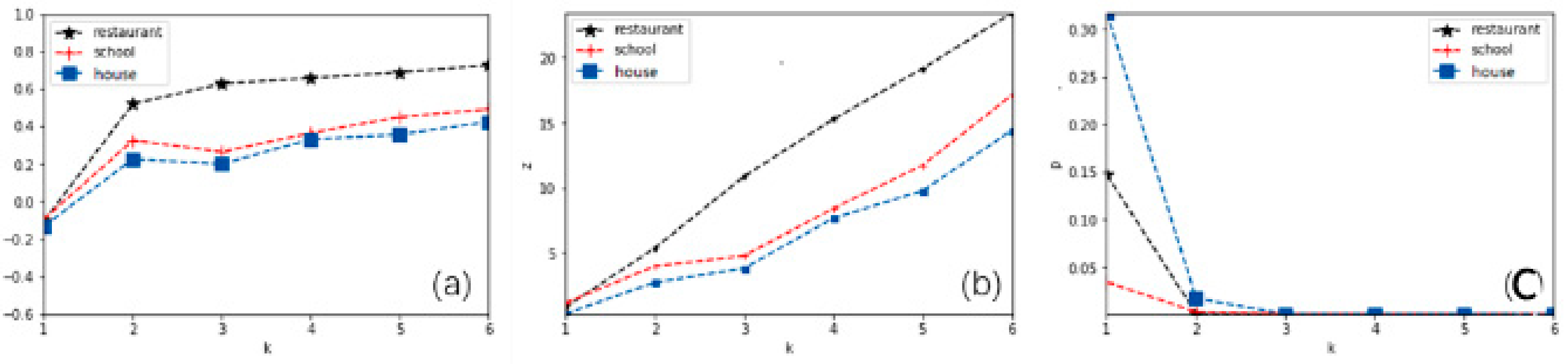
| I | -0.131 | 0.227 | 0.201 | 0.332 | 0.358 | 0.425 |
| p | 0.181 | 0.001 | 0.014 | 0.001 | 0.001 | 0.001 |
| z | 0.353 | 2.667 | 3.796 | 8.071 | 10.116 | 13.909 |
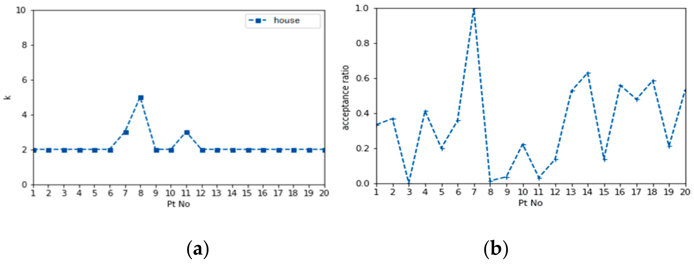
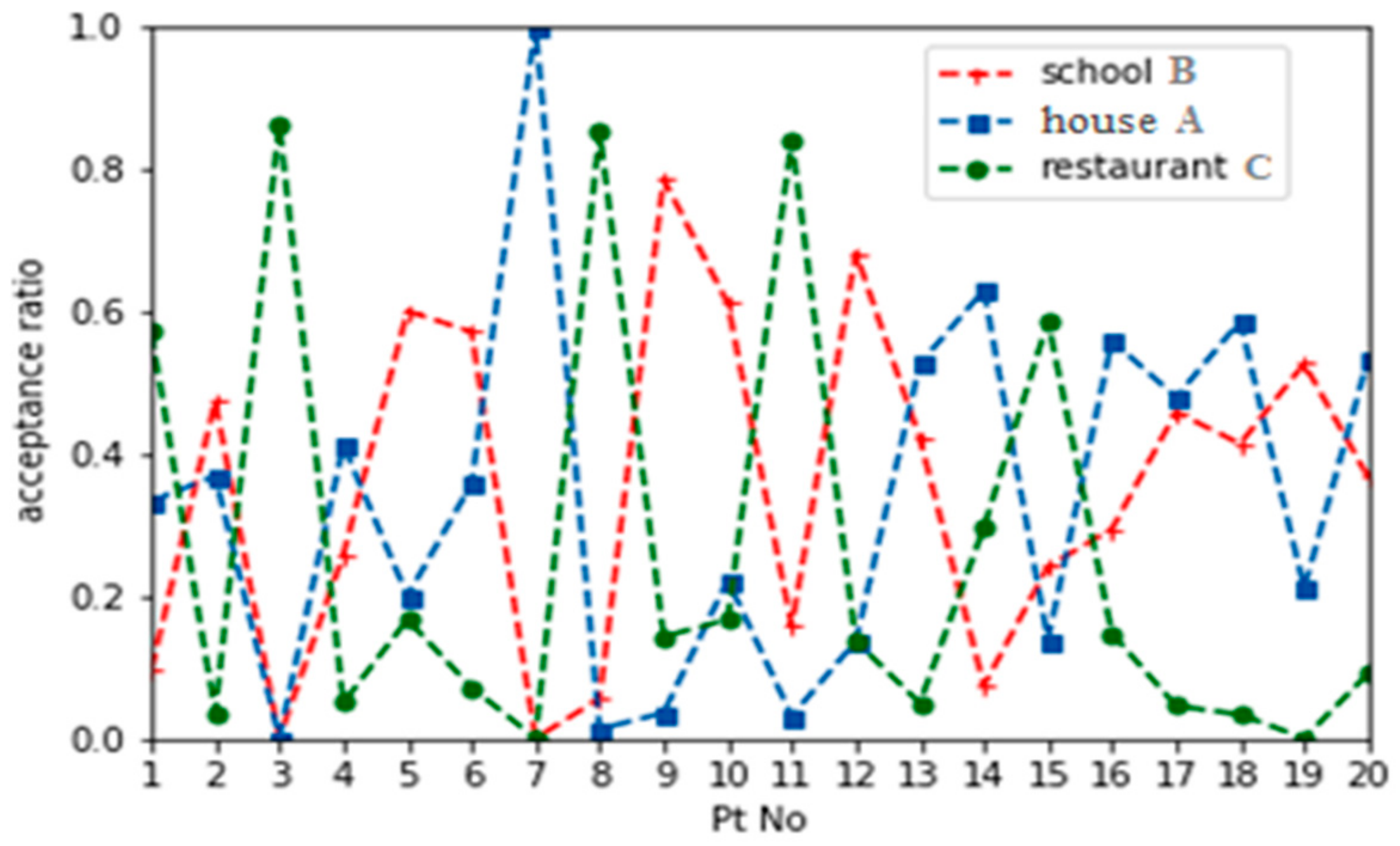
| Pt ID | 1 | 2 | 3 | 4 | 5 | 6 | 7 | 8 | 9 | 10 |
|---|---|---|---|---|---|---|---|---|---|---|
| K | 2 | 2 | 2 | 2 | 2 | 2 | 3 | 5 | 2 | 2 |
| Similar GTAs | 7 | 7 | 0 | 7 | 6 | 10 | 33 | 1 | 1 | 4 |
| DGACR’ GTAs | 21 | 19 | 21 | 17 | 30 | 28 | 33 | 78 | 28 | 18 |
| Ratio | 0.33 | 0.37 | 0 | 0.41 | 0.2 | 0.36 | 1 | 0.01 | 0.04 | 0.22 |
| Correlated or not | Y | Y | N | Y | Y | Y | Y | Y | Y | Y |
| Pt ID | 11 | 12 | 13 | 14 | 15 | 16 | 17 | 18 | 19 | 20 |
|---|---|---|---|---|---|---|---|---|---|---|
| K | 3 | 2 | 2 | 2 | 2 | 2 | 2 | 2 | 2 | 2 |
| Similar GTAs | 1 | 3 | 10 | 17 | 4 | 19 | 23 | 17 | 4 | 16 |
| DGACR’ GTAs | 32 | 22 | 19 | 27 | 29 | 34 | 48 | 29 | 19 | 30 |
| Ratio | 0.03 | 0.14 | 0.53 | 0.63 | 0.14 | 0.56 | 0.48 | 0.59 | 0.21 | 0.53 |
| Correlated or not | Y | Y | Y | Y | Y | Y | Y | Y | Y | Y |
© 2020 by the authors. Licensee MDPI, Basel, Switzerland. This article is an open access article distributed under the terms and conditions of the Creative Commons Attribution (CC BY) license (http://creativecommons.org/licenses/by/4.0/).
Share and Cite
He, Y.; Sheng, Y.; Jing, Y.; Yin, Y.; Hasnain, A. Uncorrelated Geo-Text Inhibition Method Based on Voronoi K-Order and Spatial Correlations in Web Maps. ISPRS Int. J. Geo-Inf. 2020, 9, 381. https://0-doi-org.brum.beds.ac.uk/10.3390/ijgi9060381
He Y, Sheng Y, Jing Y, Yin Y, Hasnain A. Uncorrelated Geo-Text Inhibition Method Based on Voronoi K-Order and Spatial Correlations in Web Maps. ISPRS International Journal of Geo-Information. 2020; 9(6):381. https://0-doi-org.brum.beds.ac.uk/10.3390/ijgi9060381
Chicago/Turabian StyleHe, Yufeng, Yehua Sheng, Yunqing Jing, Yue Yin, and Ahmad Hasnain. 2020. "Uncorrelated Geo-Text Inhibition Method Based on Voronoi K-Order and Spatial Correlations in Web Maps" ISPRS International Journal of Geo-Information 9, no. 6: 381. https://0-doi-org.brum.beds.ac.uk/10.3390/ijgi9060381