National-Scale Landslide Susceptibility Mapping in Austria Using Fuzzy Best-Worst Multi-Criteria Decision-Making

Abstract

Landslides are one of the most detrimental geological disasters that intimidate human lives along with severe damages to infrastructures and they mostly occur in the mountainous regions across the globe. Landslide susceptibility mapping (LSM) serves as a key step in assessing potential areas that are prone to landslides and could have an impact on decreasing the possible damages. The application of the fuzzy best-worst multi-criteria decision-making (FBWM) method was applied for LSM in Austria. Further, the role of employing a few numbers of pairwise comparisons on LSM was investigated by comparing the FBWM and Fuzzy Analytical Hierarchical Process (FAHP). For this study, a wide range of data was sourced from the Geological Survey of Austria, the Austrian Land Information System, Humanitarian OpenStreetMap Team, and remotely sensed data were collected. We used nine conditioning factors that were based on the previous studies and geomorphological characteristics of Austria, such as elevation, slope, slope aspect, lithology, rainfall, land cover, distance to drainage, distance to roads, and distance to faults. Based on the evaluation of experts, the slope conditioning factor was chosen as the best criterion (highest impact on LSM) and the distance to roads was considered as the worst criterion (lowest impact on LSM). LSM was generated for the region based on the best and worst criterion. The findings show the robustness of FBWM in landslide susceptibility mapping. Additionally, using fewer pairwise comparisons revealed that the FBWM can obtain higher accuracy as compared to FAHP. The finding of this research can help authorities and decision-makers to provide effective strategies and plans for landslide prevention and mitigation at the national level.

1. Introduction

In recent years, natural hazards have occurred quite frequently [1]. Landslides, which threaten human life and property, are considered as one of the most detrimental geological disasters that frequently occur in the mountainous area [2,3]. Landslides are defined as the downslope mass-displacement of earth, debris, and rock, because of gravity impact [4,5]. It has proven that landslides have an important role in the environmental, social, economic, and cultural sustainability of human beings [6]. Landslides occur in different sizes and shapes and are triggered by diverse factors such as earthquakes, rainfall, volcanic eruptions, and slope erosion [7]. It is predicted that the occurrence of landslides will increase in the future because of various factors, such as infrastructure development, population growth, and mistreatment of natural resources [1,8]. Landslides can be considered as a natural phenomenon that is often triggered by the impact of human undertakings [9]. The scientific community has significantly seen an upturn in the novel approaches being considered for the assessment of landslides due to the alarming increase of landslides across the globe [10]. It is vital to study the region’s susceptibility to landslides to understand the impact of various factors influencing the occurrences of landslides. Landslide susceptibility mapping (LSM) is the quantification of the likelihood of incidences of landslides depending on the impact of the various conditioning factors in the given region [11]. The LSM is pivotal in managing the landslides and there are diverse approaches used for deriving landslide susceptibility maps [7,12]. LSM mainly wishes to measure, map, and eventually comprehend the spatial distribution of the occurrences of landslides in the future [13]. There has been very little research on landslide susceptibility done at the national scale, rather focusing more on the regional scale [14].The LSM can help authorities and decision makers to plan effective management strategies for landslide prevention and mitigation [15,16].

Geographic information systems (GIS) have been proven to be a robust tool for studying various natural hazards, including landslides, such as preparation of inventory data, landslide susceptibility mapping, and landslide detection [17,18,19]. Remote sensing (RS) have also contributed to augmented assistance in mitigating and planning of natural hazards [20]. Multi-criteria decision making (MCDM) is a broadly accepted approach that has been applied in a wide range of issues in diverse fields, which also includes studies on LSM. The integration of GIS and the MCDM approach allows for converting spatial as well as non-spatial data into meaningful information. Analytical hierarchical process (AHP) assessment is a multi-criteria expert-based approach that is widely used in susceptibility mapping [21,22]. However, the AHP approach has some gaps and limitations, such as ignoring the interrelations among the different causes at different levels, low performance in the case of 5 × 5 or larger Pairwise Comparisons, and the eigenvector optimality problem [23]. Some of the limitations and inabilities of the application of the AHP in the spatial decision support systems are described by [24,25,26,27,28]. The Fuzzy set theory, mimicking human judgment, has been designed to reduce inconsistency and uncertainty in decisions as well as overcoming the limitations of AHP [29]. In this regard, several fuzzy-based methods have been introduced and implemented in different fields in recent years; the successful application of the Fuzzy Analytical hierarchical process (FAHP) method in LSM can be an example.

The best-worst multi-criteria decision-making method (BWM) is one of the latest MCDM models created by Rezaei in 2015 [30]. It seeks to overcome the inconsistency derived from pairwise comparisons by minimizing the pairwise comparisons as well as obtaining the weights of criteria and alternatives with respect to different criteria [31]. Even though the BWM uses a 1–9 scale to perform the pairwise comparisons, like AHP, it only executes the preference of the best and the worst criteria over all the other criteria that are completely different from AHP. Because the secondary comparisons are not executed in this method, it is much more comfortable, more precise, and has lesser redundancy. However, expert knowledge and judgment, which usually hold some drawbacks, such as ambiguity and uncertainty into the model, play an important role in the BWM method. Therefore, employing a fuzzy set theory, which may be more in line with real-world situations and can achieve better results, is considered an efficient solution. However, expert knowledge and judgment, which usually hold some drawbacks, such as ambiguity and uncertainty into the model, play an important role in the BWM method [27]. Therefore, employing a fuzzy set theory, which might be more in line with real-world situations and can achieve better results, is considered to be an efficient solution [23].

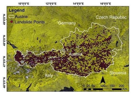
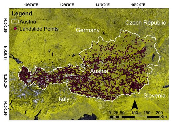
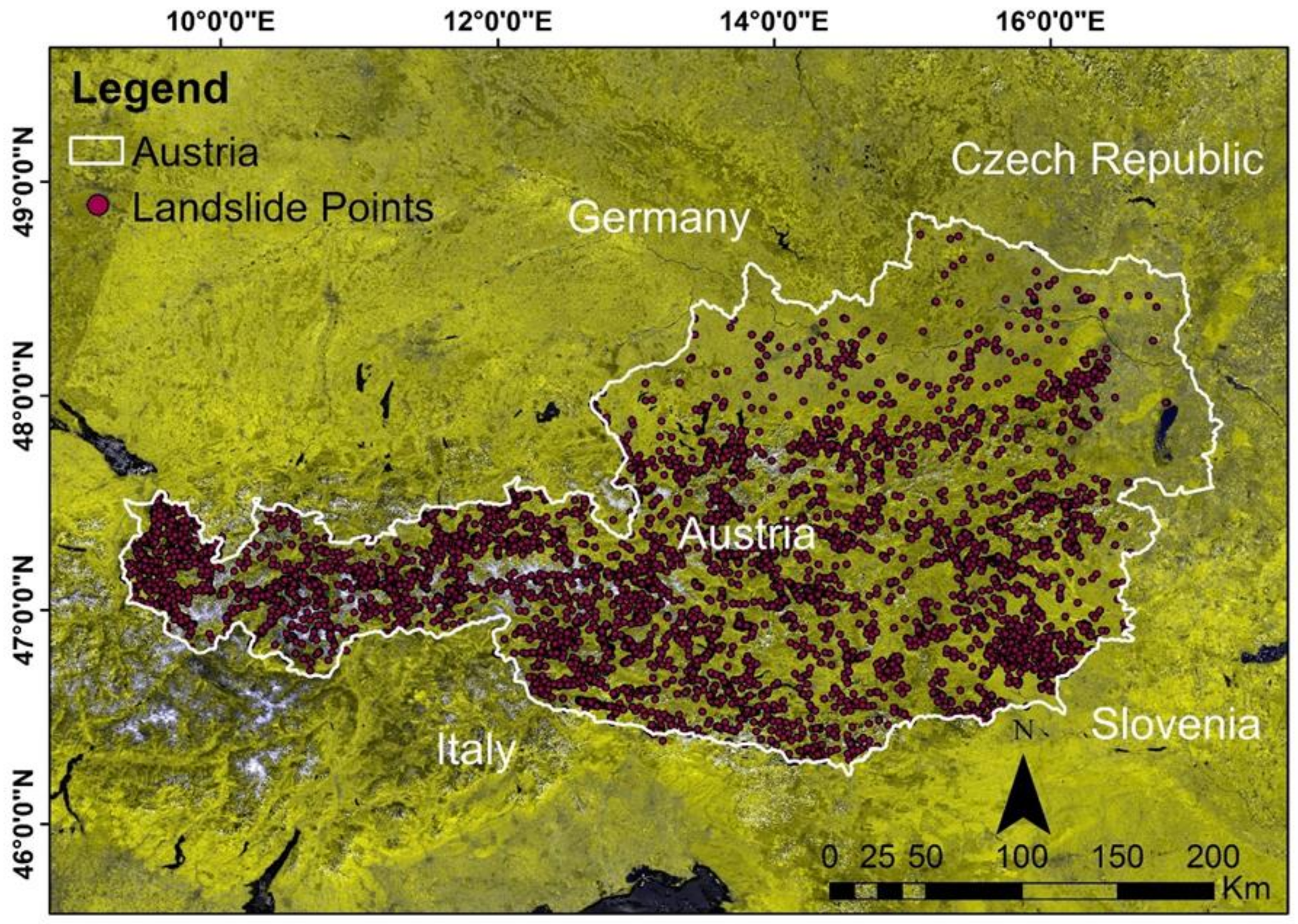
In an alpine and mountainous country, like Austria, mass movements or landslides are a prevalent natural hazard [32]. Several studies were carried out assessing land susceptibility map at national scales worldwide, mostly focusing on fewer conditioning factors and statistical approaches [9,33,34,35,36,37]. For example, while applying seven factors and hybrid methods, Suh and others (2011) generated a national-scale assessment of landslide susceptibility of rock-cut slopes along expressways in Korea [35]. Trigila and others (2013) used different models (logistic regression, discriminant analysis, and Bayesian tree random forest) to produce an LSM in Italy [34]. In 2011, an LSM for Romania was obtained using seven main factors and landslide susceptibility index by Balteanu and others. In the case of Austria, there are two studies that have been carried out for entire Austria [38,39]; however, there remain some challenges in terms of susceptibility mapping and the approaches used [40]. This paper aims to investigate the application of fuzzy best-worst multi-criteria decision-making (FBWM) for generating an LSM at a national scale that has not yet been carried out to date, to our best knowledge. This study is quite relevant to the present scenario, where there have been heavy landslides in Austria causing several mortalities and major economic losses. This study also investigates the role of employing a few numbers of pairwise comparisons on LSM by comparing FBWM and FAHP.

2. Material

2.1. Overview of the Study Area

Austria, covering an area of 83,879 km² and lying between longitudes 9° and 18° E and latitudes 46° and 49° N, is a landlocked country of nearly nine million citizens in Central Europe (see Figure 1). Landslides often occur in the country because of its geomorphological setting. River flooding, soil erosion debris flows/mountain torrents, avalanches, and landslides are introduced as the most life-threatening geological disasters in Austria by Hamann (2007) [41]. In Austria, the elevation varies between 110 m and 3800 m, and only 32% of the country is below 500 m. Besides, the Northern Limestone Alps, Central Eastern Alps, and the Southern Limestone Alps are mostly located in the country. Those mountainous parts are prone to rock falls, colossal mass movement, and landslides, causing a loss of lives and damage to infrastructure. The mean annual rainfall per year varies depending on the regions in Austria; it ranges between 400 mm and 600 mm in eastern regions that are flat or hilly, while this amount exceeds 2000 mm in alpine regions.

2.2. Data

2.2.1. Landslide Inventory Data

The mapping of actual landslides in the study area is vital in describing the relationship between condition factors and landslide distribution [42]. The inventory for landslides in Austria was provided by the Geological Survey of Austria. There have been substantial occurrences of landslides in Austria, the inventory data from Geological Survey of Austria does not include all of the landslides and has limitations regarding completeness and up-to-datedness. The data obtained from GBA for landslides is the inventory data used for validating and comparing the performance of FBWM and FAHP. There are about 6309 landslide point inventory data available from GBA for Austria as of March 2019, which mainly comprises of rockfalls/rockslides (25%), complex movements (6%), and landslides (69%). More information can be found at GBA (www.geologie.ac.at).

2.2.2. Landslide Conditioning Factors

Meanwhile, there are no globally accepted predefined criteria for choosing condition factors, the conditioning factors should ideally be quantifiable, non-uniform, operative, and non-redundant [43]. For this study, we used nine conditioning factors that were based on the previous literature, expert feedback, and geomorphological characteristics of Austria, such as slope, elevation, slope aspect, distance to drainage, distance to roads, distance to faults, lithology, land cover, and rainfall (

Table 1. A summary of the literature review of the importance of landslide conditioning factors.

No	Factors	Impacts	References
1	Elevation	The elevation is a critical factor in landslide occurrence due to the huge variability in climate and weather conditions at different elevations that can lead variances in vegetation and soil.	Mahdadi et al. 2018 [44]; Conoscenti et al. 2016 [45]
2	Slope	The slope angle has a great impact on landslide events; a larger slope angle is more susceptible to failure.	Ghorbanzadeh et al. 2019 [46,47]
3	Slope aspect	The slope aspect, which often controls the amount of water in the hillsides and slopes, influences the slope steadiness.	Shahabi et al., 2014; Pourghasemi et al., 2018 [8,48]
4	Distance to drainage/rivers	It has proven that closer areas to drainage have more soil erosion and as a result higher risk of landslides. Besides, higher wet conditions affect the stability and the underground flow.	Haris et al., 2014 [49]; Paraskevas and Ioanna [50]
5	Distance to roads	Roads often cut the slope, affect slope stability, and change the surface morphology.	Yan et al. 2018 [51]
6	Distance to faults	Since earthquakes have critical roles in cracking of stones that, in turn, cause instability, active faults can be considered as an effective issue in landslides.	Chen et al., 2017 [18]
7	Lithology	Landslides occurrence is under the influence of lithology units because they determine permeability, strength, and susceptibility to failure.	Yalcin et al. 2007 [52]; Segoni et al. 2020 [53]
8	Land cover	The spatial distribution of land cover types affects the propensity of landslide occurrence.	Meneses et al. 2019 [54]
9	Rainfall	Annual rainfall has introduced as the main triggering factor for landslides occurring in Austria. Rainfall amount, varying by topographical characteristics and weather conditions, can trigger landslides.	Bui DT et al. 2013 [55]

). The freely available 10 m resolution digital elevation model (DEM) was downloaded from the Austrian open data portal (www.data.gv.at). The slope and aspect were derived from the DEM data. The lithology and distance to fault data were obtained from the Geological Survey of Austria. The land cover data was downloaded from the Land Information System Austria. The drainage and road networks were downloaded from the humanitarian open street map network. Rainfall data for Austria was obtained from the ÖKS15—Klimaszenarien für Österreich. All of the data were converted to 10 m resolution for consistency and for the further processing of the data. This was carried out using Environmental Systems Research Institute (ESRI) ArcGIS platform to generate the conditioning factors of LSM in Austria.

3. Methods

The methodology of present research contains three stages, as follows: (1) Deterring the criteria affecting LSM and submitting them to experts for initial ranking and identifying the best criterion and the worst criterion (see Section 2.2.2). (2) Implementing the FBWM and FAHP to generate LSM. (3) Validation FBWM and FAHP using the Receiver operating characteristic curve (ROC) and area under the curve (AUC). (4) Comparison of generated landslide susceptibility maps.

3.1. Fuzzy Best–Worst Method

The Best–Worst Method (BWM) was suggested by Rezaei [30], where he demonstrated that the MCDM problems might be resolved by pairwise comparisons having a very low number [56]. In the proposed method, the user selects the most important criterion and the least important criterion from all of the criterions available and the best or the most important criterion is then compared with all other criteria and assigned a number in the range between 1 to 9, where 1 represents that the criterion is as important as the best or most important criterion, and 9 represents that the best criterion is nine times more important than the worst criterion [57]. Likewise, the comparison is done for the least or the worst important criterion, with all the other criteria. These numbers or values are then used for an optimization process [58]. The objective of this optimization process is to gain the maximum degree of consistency via minimizing the maximum difference between the best-criterion-to-any-criterion comparison value and the ratio of the weights of the best criterion and that criterion. It also targets minimizing the maximum difference between the any-criterion-to-worst-criterion comparison value and the ratio of the weights of that particular criterion and the worst criterion. This optimization is done by some more value constraints, such as the maximum possible value of the sum of the weights.

Generating LSM in Austria, we applied FBWM that contains six main steps in order to determine the weights of the criteria, as follows:

Phase 1. Generate the decision criteria system. As the values of decision criteria have an impact on the performances of different alternatives, generating the decision criteria system, which involves a set of decision criteria, is considered a vital step for realistically performing the assessment on alternatives.

Phase 2. Defining the best criterion (the most important) and the worst criterion (the least important). In this step, based on experts’ opinions, the best criterion and the worst criterion should be identified.

Phase 3. Determining the fuzzy preference of the best criterion against all other criteria. In this section, applying the linguistic terms of experts that are listed in

Table 2. Transformation instructions of linguistic variables of experts.

Linguistic Terms	Membership Function
Equally importance (EI)	(1, 1, 1)
Weakly important (WI)	(2/3, 1, 3/2)
Fairly Important (FI)	(3/2, 2, 5/2)
Very important (VI)	(5/2, 3, 7/2)
Absolutely important (AI)	(7/2, 4, 9/2)

, the fuzzy preference of the best criterion against all the other criteria can be identified. Subsequently, based on the transformation rules that are shown in Table 1, the acquired fuzzy preferences are transformed to TFNs. The achieved fuzzy best criterion -to-others vector is:

$${\tilde{A}}_B=\left({\tilde{a}}_{B1}, {\tilde{a}}_{B2}, \dots , {\tilde{a}}_{Bn}\right)$$

(1)

where ${\tilde{A}}_B$ symbolizes the fuzzy best criterion -to-others vector and ${\tilde{a}}_{Bj}$ symbolizes the fuzzy preference of the most important criterion $c_B$ over criterion j, j = 1, 2, ···, n.

Phase 4. Determining the fuzzy preference of the worst criterion against all other criteria. In this step, imitating the previous step, the fuzzy preference of the worst criterion against all the other criteria is identified. The achieved fuzzy worst criterion-to-others vector is:

$${\tilde{A}}_W=\left({\tilde{a}}_{1W}, {\tilde{a}}_{2W}, \dots , {\tilde{a}}_{nW}\right)$$

(2)

where ${\tilde{A}}_W$ symbolizes the fuzzy worst criterion-to-others vector and ${\tilde{a}}_{iW}$ symbolizes the fuzzy preference of the least important criterion i over criterion $c_W$, i = 1, 2, ···, n.

Phase 5. Defining the ideal fuzzy weights. The ideal fuzzy weights for each criterion $\left({\tilde{W}}_1^{\ast }, {\tilde{W}}_2^{\ast },\dots ,W_n^{\ast }\right)$ can be reached when for each fuzzy pair ${\tilde{w}}_B/{\tilde{w}}_j={\tilde{a}}_{Bj}$ and ${\tilde{w}}_j/{\tilde{w}}_W={\tilde{a}}_{jW}$. To obtain these conditions, the maximum absolute gaps $\left|\frac{{\tilde{w}}_j}{{\tilde{w}}_W}-{\tilde{a}}_{jW}\right|$ and $\left|\frac{{\tilde{w}}_B}{{\tilde{w}}_j}-{\tilde{a}}_{Bj}\right|$ for all j should be minimized (see Equation (3)). Transforming the crisp value of fuzzy weight $\tilde{w}$ is another section that should be done in this phase; in this study, the graded mean integration representation was used to this end (see Equation (4)).

$$min {\tilde{\xi }}^{\ast } s.t.\left\{\begin{array}{l}\left|\frac{\left(l_B^w,m_B^w,u_B^w\right)}{\left(l_j^w,m_j^w,u_j^w\right)}-\left(l_{Bj},m_{Bj},u_{Bj}\right)\right|\le \left(k^{\ast },k^{\ast },k^{\ast }\right)\\ \left|\frac{\left(l_j^w,m_j^w,u_j^w\right)}{\left(l_W^w,m_W^w,u_W^w\right)}-\left(l_{jW},m_{jW},u_{jW}\right)\right|\le \left(k^{\ast },k^{\ast },k^{\ast }\right)\\ {\displaystyle {\displaystyle \sum }_{j=1}^n}R\left({\tilde{w}}_j\right)=1\\ l_j^w\le m_j^w\le u_j^w\\ l_j^w\ge 0\\ j=1,2,\dots ,n\end{array}\right.$$

(3)

$$R_{\left({\tilde{a}}_i\right)}=\frac{l_i+4m_i+u_i}{6}$$

(4)

Phase 6. Analyzing the consistency ratio (CR). CR is considered to be a vital indicator to assess the consistency ratio of pairwise comparisons. A fuzzy comparison can be counted as fully consistent when ${\tilde{a}}_{Bj}\times {\tilde{a}}_{jW}={\tilde{a}}_{BW}$, where ${\tilde{a}}_{BW}$ , ${\tilde{a}}_{jW}, \mathrm{and} {\tilde{a}}_{Bj}$ are the fuzzy preference of the best criterion against the worst criterion, the fuzzy preference of the best criterion against the criterion j, and the fuzzy preference of the criterion j against the worst criterion, respectively. In general, the CR can be calculated for FBWM, as follows:

$${\tilde{\xi }}^2-\left(1+2u_{BW}\right)\tilde{\xi }+\left(u_{BW}^2-u_{BW}\right)=0$$

(5)

where $\xi =\left(l^{\xi },m^{\xi },u^{\xi }\right), {\tilde{a}}_{BW}=\left(l_{BW},m_{BW},u_{BW}\right)$.

The maximum possible $\xi$ can be reached, which is implemented as the consistency index (CI) for fuzzy BWM, by solving Equation (5) for dissimilar $u_{BW}$. When considering different linguistic terms of expert’s opinions, the obtained CI for FBWM is listed in

Table 3. Consistency index for fuzzy BWM.

Linguistic Terms	EI	WI	FI	VI	AI
${\tilde{a}}_{BW}$	(1, 1, 1)	(2/3, 1, 3/2)	(3/2, 2, 5/2)	(5/2, 3, 7/2)	(7/2, 4, 9/2)
CI	3	3.8	5.29	6.69	8.04

.

3.2. Fuzzy Analytical Hierarchical Process (FAHP)

Fuzzy analytical hierarchical process has been widely used in recent years in order to deal with uncertainty and fuzziness in the multi criteria decision making. The approach of FAHP entails utilization of scientific approach where the weights are derived through fuzzy pair wise comparisons matrices [59]. There are various approaches of FAHP used by researchers for diverse applications transportation [60]. 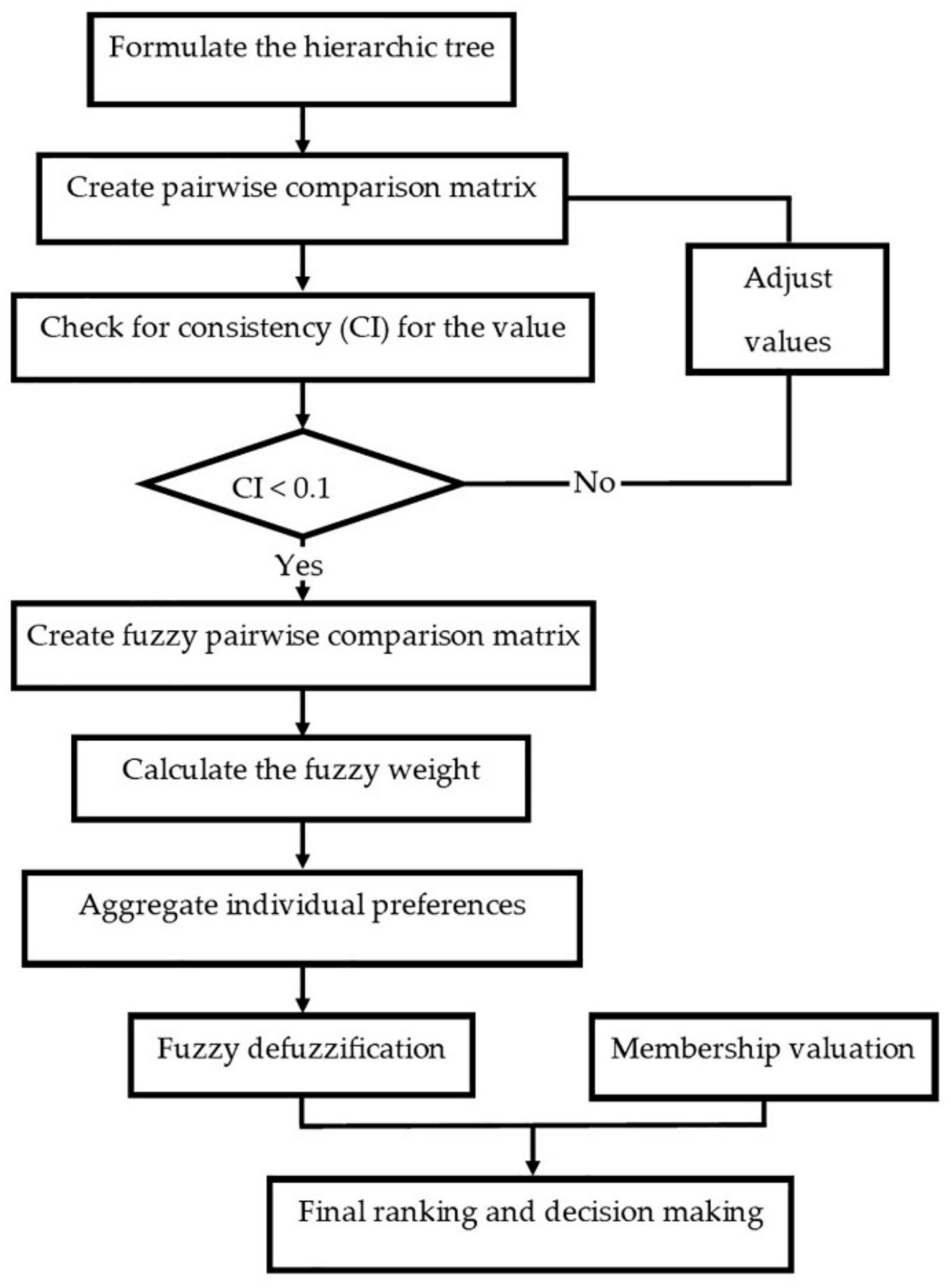A novel approach of synthetic extent standards for handling FAHP through pairwise comparison was proposed [61]. For this study, a method for synthesized multi-index analysis using FAHP analysis to define index weight was used. An eight-step procedure describing FAHP is provided in Figure 2, whilst a detailed description of the methodology is presented in Figure 3.

By using the fuzzy sets theory, it is possible to consider more than one susceptible class while using the concept of partial membership. Based on this perspective, the spatial variability was analyzed using the fuzzy membership functions. The practice of fuzzy sets theory in landslide assessment has been considered to improve the resulting susceptibility mapping. Consequently, all of the landslide initiating factors were harmonized in range of 0 (low susceptible) to 1 (high susceptible).

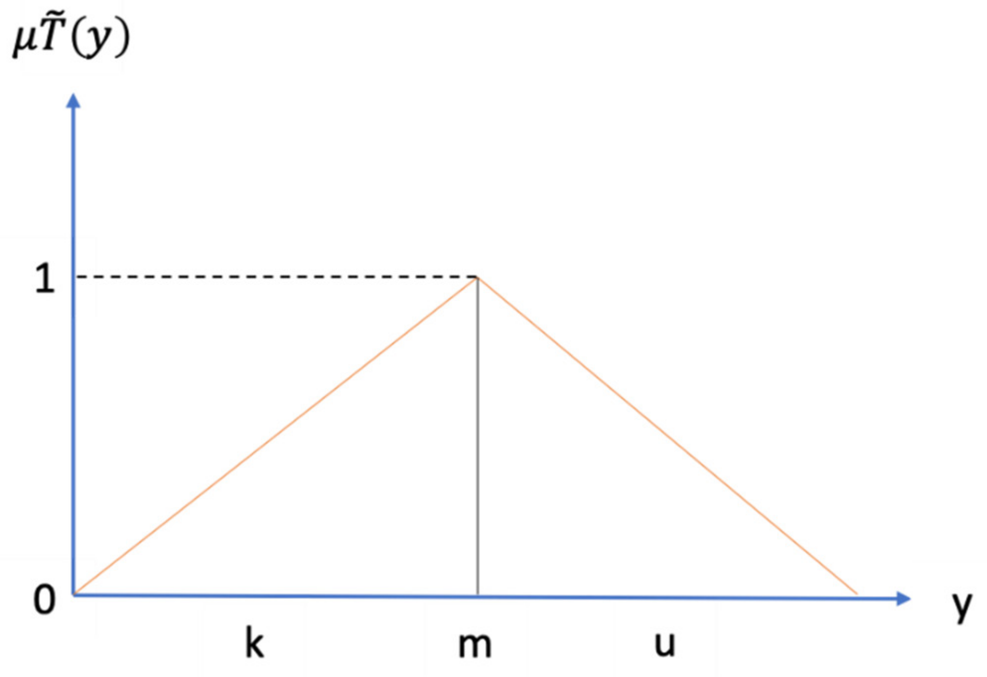
A fuzzy number $\tilde{T}$ on $\mathbb{R}$ to be a triangular fuzzy number if its membership function $\mu \tilde{T}\left(y\right): \mathbb{R}\to \left[0,1\right]$ is equal to the following formula (6):

$$\mu \tilde{T}\left(y\right)=\left\{\begin{array}{c}\frac{y-1}{m-1}, k\le y\le m\\ \frac{u-y}{u-m}, m\le y\le u\\ 0, \mathrm{otherwise}\end{array}\right.$$

(6)

From formula (1), $k$ and $u$ mean the lower and upper bounds of the fuzzy number $\tilde{A}$ and $m$ is the modal value for $\tilde{A}$. The triangular fuzzy number can be denoted by $\tilde{T}=\left(k, m, u\right)$. The operational laws of triangular fuzzy number $\tilde{T}{ }_1=\left(k_1, m_1, u_1\right)$ and $\tilde{T}{ }_2=\left(k_2, m_2, u_2\right)$ are displayed as following Equations (7)–(11). Addition of the fuzzy number $⨁$

$$\tilde{T}{ }_1 ⨁\tilde{T}{ }_2=\left(k_1+k_2,m_1+m_2,u_1+u_2\right)$$

(7)

A triangular fuzzy set was utilized for transforming the linguistic variables to the quantitative values for this study, as shown n Figure 2.

Multiplication of the fuzzy number $⨂$

$$T{ }_1 ⨂\tilde{T}{ }_2=\left(k_1{k}_2, m_1{m}_2, u_1{u}_2\right) \mathrm{for} k_1, k_2>0;m_1,m_2>0;u_1{u}_2>0$$

(8)

Subtraction of the fuzzy number $⊝$

$$\tilde{T}{ }_1 ⊝\tilde{T}{ }_2=\left(k_1-u_2, m_1-,m_2, u_1-k_2\right)$$

(9)

Division of a fuzzy number $\varnothing$

$$\tilde{T}{ }_1 \varnothing \tilde{T}{ }_2=\left(\frac{k_1}{u_2},\frac{m_1}{,m_2},\frac{u_1}{l_2}\right)\mathrm{for} k_1, k_2>0;m_1,m_2>0;u_1{u}_2>0$$

(10)

Reciprocal of the fuzzy number

$$\tilde{T}{ }^{-1}=\left(\frac{1}{u_1},\frac{1}{m_1},\frac{1}{ k_1}\right) \mathrm{for} k_1, k_2>0;m_1,m_2>0;u_1{u}_2>0$$

(11)

For this study, we used the triangular fuzzy numbers scale which is a computational technique was used.

Table 4. This shows the relationship between the quantitative values and the linguistic variables.

Fuzzy Number	Linguistic Variables	Triangular Fuzzy Numbers
9	Perfect	(8, 9, 10)
8	Absolute	(7, 8, 9)
7	Very good	(6, 7, 8)
6	Fairly good	(5, 6, 7)
5	Good	(4, 5, 6)
4	Preferable	(3, 4, 5)
3	Not bad	(2, 3, 4)
2	Weak advantage	(1, 2, 3)
1	Equal	(1, 1, 1)

shows the triangular fuzzy numbers scale [62].

The engaged pairwise comparison matrices are crafted based on the hierarchical structure. Pairwise comparisons are crafted by assigning linguistic terms to equate which criteria are the more important than the other with respect to the main one, as $T$ the bigger matrix ($6\times 6$) in the study, as presented below in Equation (12):

$$\tilde{T}=\left[\begin{array}{cc}\begin{array}{ccc}1& {\tilde{a}}_{12}& {\tilde{a}}_{13}\\ {\tilde{a}}_{21}& 1& {\tilde{a}}_{23}\\ {\tilde{a}}_{31}& {\tilde{a}}_{32}& 1\end{array}& \begin{array}{ccc}{\tilde{a}}_{14}& {\tilde{a}}_{15}& {\tilde{a}}_{16}\\ {\tilde{a}}_{24}& {\tilde{a}}_{25}& {\tilde{a}}_{26}\\ {\tilde{a}}_{34}& {\tilde{a}}_{35}& {\tilde{a}}_{36}\end{array}\\ \begin{array}{ccc}{\tilde{a}}_{41}& {\tilde{a}}_{42}& {\tilde{a}}_{43}\\ {\tilde{a}}_{51}& {\tilde{a}}_{52}& {\tilde{a}}_{53}\\ {\tilde{a}}_{61}& {\tilde{a}}_{62}& {\tilde{a}}_{63}\end{array}& \begin{array}{ccc}1& {\tilde{a}}_{45}& {\tilde{a}}_{46}\\ {\tilde{a}}_{54}& 1& {\tilde{a}}_{56}\\ {\tilde{a}}_{64}& {\tilde{a}}_{65}& 1\end{array}\end{array}\right]=\left[\begin{array}{cc}\begin{array}{ccc}1& {\tilde{a}}_{12}& {\tilde{a}}_{13}\\ 1/{\tilde{a}}_{12}& 1& {\tilde{a}}_{23}\\ 1/{\tilde{a}}_{13}& 1/{\tilde{a}}_{23}& 1\end{array}& \begin{array}{ccc}{\tilde{a}}_{14}& {\tilde{a}}_{15}& {\tilde{a}}_{16}\\ {\tilde{a}}_{24}& {\tilde{a}}_{25}& {\tilde{a}}_{26}\\ {\tilde{a}}_{34}& {\tilde{a}}_{35}& {\tilde{a}}_{36}\end{array}\\ \begin{array}{ccc}1/{\tilde{a}}_{14}& 1/{\tilde{a}}_{24}& 1/{\tilde{a}}_{34}\\ 1/{\tilde{a}}_{15}& 1/{\tilde{a}}_{25}& 1/{\tilde{a}}_{35}\\ 1/{\tilde{a}}_{16}& 1/{\tilde{a}}_{26}& 1/{\tilde{a}}_{36}\end{array}& \begin{array}{ccc}1& {\tilde{a}}_{45}& {\tilde{a}}_{46}\\ 1/{\tilde{a}}_{45}& 1& {\tilde{a}}_{56}\\ 1/{\tilde{a}}_{46}& 1/{\tilde{a}}_{56}& 1\end{array}\end{array}\right]$$

(12)

where

$${\tilde{a}}_{ij}=\left\{\begin{array}{ll}{\tilde{9}}^{-1}, {\tilde{8}}^{-1},{\tilde{7}}^{-1},{\tilde{6}}^{-1},{\tilde{5}}^{-1},{\tilde{4}}^{-1},{\tilde{3}}^{-1},{\tilde{2}}^{-1},\tilde{1},\tilde{2},\tilde{3},\tilde{4},\tilde{5},\tilde{6},\tilde{7},\tilde{8},\tilde{9},& 1,i\ne j\\ 1& i=j\end{array}\right.$$

where a $ij$ is fuzzy comparison value of dimension $i$ to criterion j.

The fuzzy geometric mean was used for aggregating the fuzzy weights as shown in Equations (13)–(14).

$${\tilde{r}}_i={\left({\tilde{a}}_{i1} ⨂ {\tilde{a}}_{i2} ⨂{\widetilde{ a}}_{i3}⨂ {\tilde{a}}_{i4} ⨂ {\tilde{a}}_{i5} ⨂ {\tilde{a}}_{i6}\right)}^{1/n}$$

(13)

$${\tilde{w}}_i={\tilde{r}}_i {\left[{\tilde{r}}_1⨁ {\tilde{r}}_2 ⨁ {\tilde{r}}_3 ⨁ {\tilde{r}}_4 ⨁ {\tilde{r}}_5⨁ {\tilde{r}}_6\right]}^{-1}$$

(14)

${\tilde{r}}_i$ is a geometric mean of fuzzy comparison value of criterion $i$ to each criterion and ${\tilde{w}}_i$ is the fuzzy weight of the $i$th criterion that can be designated by a triangular fuzzy number, ${\tilde{w}}_i=\left(k{w}_i, m{w}_i, u{w}_i\right)$. The $k{w}_i, m{w}_i \mathrm{and} u{w}_i$ stand for the lower, middle, and upper values of the fuzzy weight of the $i$th dimension.

3.3. Receiver Operating Characteristics (ROC)

Validation is a key aspect of any analysis that enables insights into the accuracy of the models used for the study [5,63]. The relationship between the inventory data and the resulting LSM is very important for predicting the effectiveness of the model. The accuracy of the model indicates whether the model has correctly predicted the areas susceptible to landslides.

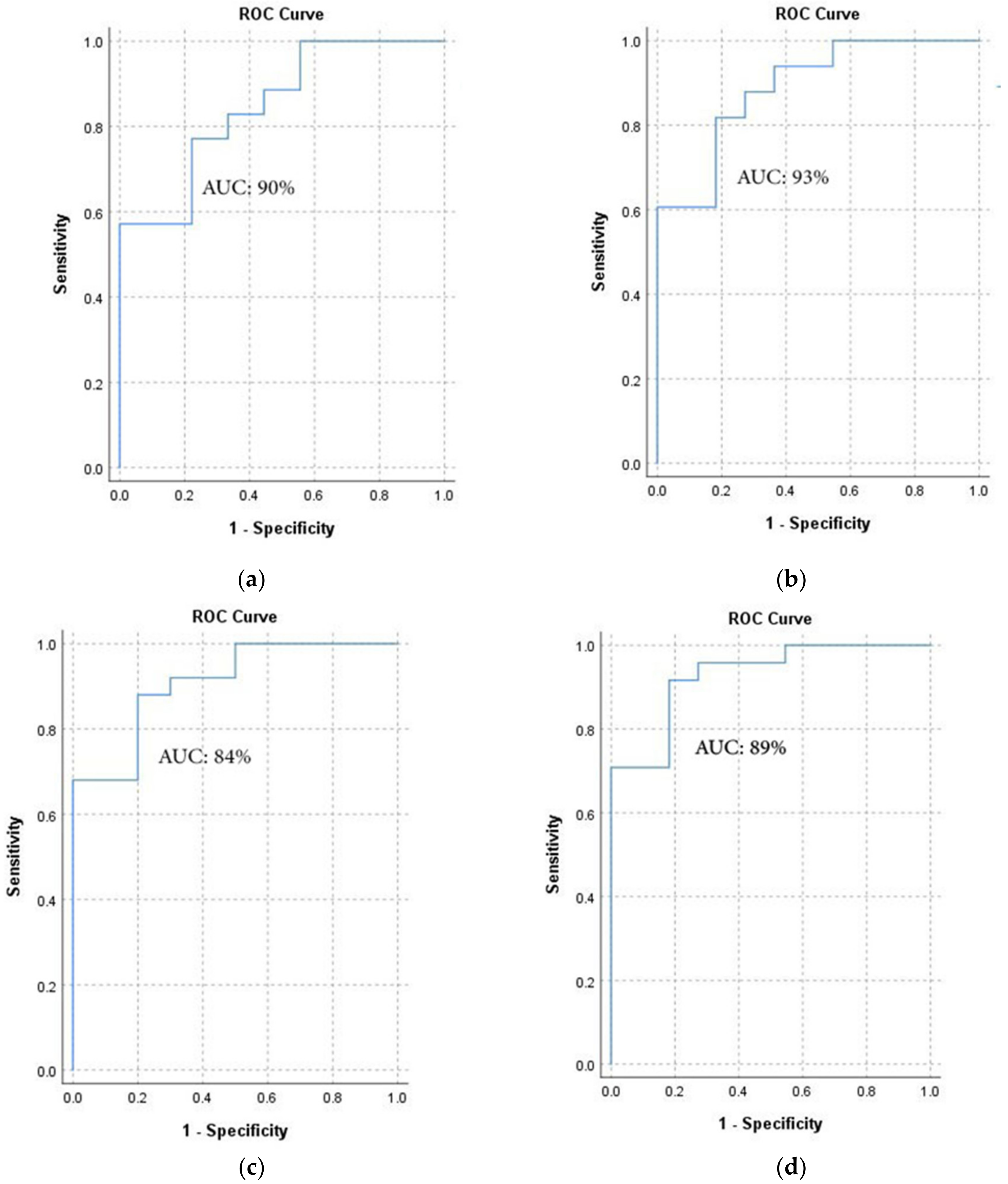
The receiver operating characteristics (ROC) curve was used for validating the resulting landslide susceptibility maps while using the validation data. The ROC approach allows for a comparison between the true positive rate and the false positive rate in the resulting landslide susceptibility maps [64,65]. ROC curves were calculated for all landslide susceptibility maps. Pixels that are correctly identified (high susceptibility) and thus match the landslide reference data are the true positive rates, while the incorrectly labeled pixels are the FPRs. ROC curves are generated by plotting the true positive rates versus the false positive rates. The area under the curve (AUC) is the degree that specifies the accuracy of the resulting landslide susceptibility maps. The AUC indicates the probability that more pixels were correctly labeled than incorrectly labeled. Greater AUC values indicate a higher accuracy and lower AUC values indicate lower accuracy of the susceptibility map. If the AUC values are close to unity, then this indicates a significant susceptibility map. A value of 0.5 shows an insignificant map, because it means that the map was generated by coincidence [66].

4. Results and Discussion

4.1. FBWM

The FBWM was used for generating the LSM for Austria. By taking experts evaluations into account, the slope criterion was chosen as the best criterion (highest impact on LSM), and the distance to roads was considered to be the worst criterion (lowest impact on LSM). Subsequently, the preference of the best and the worst criteria against all the other criteria were executed, and the global and the local values of all criteria and consistency index were obtained as indicated in

Table 5. Fuzzy best-worst multi-criteria decision-making (FBWM) model results.

Criteria/Clusters	Local Weight	Global Weight	Local Rank	Global Rank	CR
Slope (%)	0.36			1	0.041
0–10	0.041	0.01476	5	20
10–20	0.079	0.02844	4	10
20–30	0.187	0.06732	3	4
30–40	0.25	0.09	2	2
40 <	0.443	0.15948	1	1
Distance to fault (m)	0.15			2	0.075
0-1500	0.53	0.0795	1	3
1500–3000	0.26	0.039	2	7
3000–4500	0.14	0.021	3	15
450 <	0.07	0.0105	4	24
Precipitation (mm)	0.13			3	0.005
950–1725	0.061	0.00793	4	30
1725–2500	0.173	0.02249	3	14
2500–3275	0.32	0.0416	2	6
3275–4050	0.446	0.05798	1	5
Land cover	0.085			4	0.053
Forest	0.061	0.005185	7	39
Shrub land	0.072	0.00612	6	36
Grass land	0.143	0.012155	3	22
Agriculture	0.098	0.00833	4	28
Barren	0.359	0.030515	1	8
Water body	0.175	0.014875	2	19
Snow cover	0.092	0.00782	5	31
Lithology	0.082			5	0.004
Glacier	0.035	0.00287	6	41
Fluvial calcareous	0.072	0.005904	5	37
Fluvial non-calcareous	0.082	0.006724	4	34
Slate/Phyllite	0.127	0.010414	3	25
Quartzite	0.33	0.02706	2	11
Gneiss	0.354	0.029028	1	9
Aspect	0.076			6	0.051
Flat	0.11	0.00836	5	27
North	0.301	0.022876	1	13
East	0.255	0.01938	2	17
West	0.193	0.014668	3	21
South	0.141	0.010716	4	23
Elevation (m)	0.045			7	0.023
< 1000	0.16	0.0072	3	33
1000–3000	0.54	0.0243	1	12
3000–4500	0.17	0.00765	2	32
4500 <	0.13	0.00585	4	38
Distance to drainage (m)	0.038			8	0.034
< 200	0.43	0.01634	1	18
200–400	0.21	0.00798	2	29
400–600	0.165	0.00627	3	35
600–800	0.123	0.004674	4	40
800 < m	0.072	0.002736	5	42
Distance to roads (m)	0.034			9	0.025
0–150	0.61	0.02074	1	16
150–300	0.27	0.00918	2	26
300–450	0.075	0.00255	3	43
450 <	0.045	0.00153	4	44

. The global values of the criteria were acquired by multiplying the weight of the clusters by the weight of the sub-criteria. The global weight of criteria can be used for the assessment of the alternatives in the multi-criteria model [67].

The resulting susceptibility maps for landslide susceptibility were classified into five classes using natural breaks classification method. This is a widely used common method for the classification of the susceptibility maps from five classes of “Very High”,” High”, “Moderate”, “Low”, and “Very Low” [8]. This classification distributes the values into groups that contain an equal number of values. This is better than the other classifications where some classes might have a limited or excessive number of values.

The obtained LSM for Austria using FBWM illustrates that nearly 64.7% of the all landslide inventory points (4083 out of 6309) are in very high risk, 19.2 % (1212 out of 6309) in high risk, 9.9% (624 out of 6309) in moderate risk, 4.4% (277 out of 6309) in low risk, and 1.8% (113 out of 6309) in very low-risk areas, as illustrated in Figure 4.

4.2. FAHP

The FAHP approach demonstrates, as shown in

Table 6. FAHP model results.

Criteria/Clusters	Local Weight	Global Weight	Local Rank	Rank	CR
Slope (%)	0.3			1	0.052
0–10	0.017	0.0051	5
10–20	0.091	0.0273	4
20–30	0.182	0.0546	3
30–40	0.29	0.087	2
>40	0.42	0.126	1
Precipitation (mm)	0.25			2	0.011
950–1725	0.049	0.01225	4
1725–2500	0.181	0.04525	3
2500–3275	0.28	0.07	2
3275–4050	0.49	0.1225	1
Distance to fault (m)	0.108			3	0.021
0–2000	0.59	0.06372	1
2000–4000	0.29	0.03132	2
4000–6000	0.065	0.00702	3
>6000	0.055	0.00594	4
Land cover	0.102			4	0.055
Forest	0.066	0.006732	7
Shrub land	0.078	0.007956	6
Grass land	0.145	0.01479	3
Agriculture	0.10	0.0102	4
Barren	0.348	0.035496	1
Water body	0.169	0.017238	2
Snow cover	0.094	0.009588	5
Aspect	0.079			5	0.052
Flat	0.103	0.008137	5
North	0.295	0.023305	1
East	0.261	0.020619	2
West	0.189	0.014931	3
South	0.152	0.012008	4
Lithology	0.06			6	0.006
Glacier	0.010	0.0006	6
Fluvial calcareous	0.089	0.00534	5
Fluvial non-calcareous	0.092	0.00552	4
Slate/Phyllite	0.132	0.00792	3
Quartzite	0.329	0.01974	2
Gneiss	0.348	0.02088	1
Elevation (m)	0.052			7	0.025
< 1000	0.18	0.00936	3
1000–3000	0.48	0.02496	1
3000–4500	0.21	0.01092	2
>4500	0.13	0.00676	4
Distance to drainage (m)	0.041			8	0.038
< 200	0.37	0.01517	1
200–400	0.26	0.01066	2
400–600	0.148	0.006068	3
600–800	0.12	0.00492	4
>800 m	0.102	0.004182	5
Distance to roads (m)	0.008			9	0.082
0–200	0.57	0.00456	1
200–400	0.31	0.00248	2
400–600	0.104	0.000832	3
>600	0.016	0.000128	4

, that the slope criterion with 0.30 had the highest impact on landslide occurrences in Austria. The last class (>40%) of slope criterion showed the highest weight of about 0.126 on the LSM for Austria; in contrast, the last class of distance to roads (>600m) criterion with 0.000128 had the lowest impact in this regard. In some more detail, the fourth class of precipitation criterion (3275–4050 mm) weighting 0.49, the first class of distance to fault criterion (0–2000 m) weighting 0.59, the fifth class of land cover class (Barren) weighting 0.348, the second class of aspect criterion (North) weighting 0.295, Gneiss units of lithology criterion weighting 0.348, the second class of elevation criterion (1000–3000 m) weighting 0.48, the first class of distance to drainage criterion (<200 m) weighting 0.37, and finally, the first class of distance to roads criterion (0–200 m) weighting 0.57 obtained the highest rate in their groups.

The obtained LSM for Austria using FAHP illustrated that nearly 63.1% of the all landslide inventory points (3981 out of 6309) are in very high risk, 14.9 % (940 out of 6309) in high risk, 11.9% (750 out of 6309) in moderate risk, 6.6% (420 out of 6309) in low risk, and 3.5% (218 out of 6309) in very low-risk areas, as illustrated in Figure 5.

4.3. Assessment and Comparison of the Models

In the past years, several MCDM approaches have been proposed by several researchers. MCDM consists of two phases; acquisition of criteria weights and criteria values and another is an aggregation of information and ranking [58]. However, due to the complexity and the uncertainty of the objectives and the fuzziness of human thinking, the employment of fuzzy information to reflect the decision might be a better approach [68]. AHP and BWM are both MCDM approaches that are based on human qualitative expertise or judgment that can sometimes be vague and lead to ambiguity and intangibility that leads to information being uncertain or vague. Therefore, fuzzy logic employed to AHP and BWM can negate this ambiguity and have information that is in line with actual situations and can obtain convincing ranking results. For this study, we wanted to compare two fuzzy approaches of FAHP and FBWM from the MCDM approach for landslide susceptibility mapping at a national scale for Austria.

In the two resulting susceptibility maps that were derived from both FAHP and FBWM, it shows that the slope conditioning factor was the most important factor for landslide susceptibility in Austria and distance to roads is the least important conditioning factor in both FBWM and FAHP. The ROC accuracy assessment was applied to find the accuracy between the models that were applied for LSM in Austria. The ROC curve method and the AUC were applied using 6309 landslide points to evaluate the performance of FAHP and FBWM approaches. The prediction rate and success rate are two main steps in model evaluation by AUC. FBWM showed a better result than FAHP in both SR and PR (Figure 6); the AUC of the SR for the FAHP and FBWM models was 0.90, and 0.93, respectively, and the AUC of the PR for the FAHP and FBWM models was 0.84 and 0.89, respectively. The AUC amount of 0.89 for FBWM shows 89% prediction accuracy of the model. Although the models obtained reasonable prediction accuracies evaluating by the AUC, FBWM with 0.89 had higher accuracy than FAHP. In general, the FBWM model showed a better result in identifying the prone areas of the landslides in Austria. This success can be summarized in two main topics, as follows: (1) FBWM, which is a vector-based technique, needs fewer pairwise comparisons when compared to the matrix-based FAHP method. (2) The final weights derived from FBWM showed high CR, whereas, in most cases, the MCDM methods cannot obtain high CR.

When comparing the findings of the present work with literature, it revealed that both FAHP and FBWM models showed better results than the first generated LSM in Austria by Lima and others [39]; adopting statistical techniques with three different predicator sets, they achieved acceptable prediction performances that ranged from 0.76 to 0.82, which were lower than the obtained result in this work. Focusing on an object-based weighting approach and improving the results using Dempster Shafer theory, [38] study has generated a national scale LSM for entire Austria; the conducted model showed a better performance than FAHP and an equal trend with the FBWM model.

4.4. Comparison of Landslide Susceptibility Maps

In this study, susceptibility values that were obtained using the two methods have been quantitatively compared on each pixel to determine the systematic spatial pattern of the differences between obtained LSMs following the methodology proposed by Xiao and others (2020) (Xiao et al., 2020). In some more detail, the proposed method is an attempt to illustrate that the classical process of comparison among landslide susceptibility models can be extended and enhanced with substantial geomorphological aspects by focusing the comparison on the values of generated LSMs and exploring the geomorphological reasons of the differences encountered. Implementing the comparison model, first, since the FBWM model had a higher AUC, it was selected as the benchmark. Subsequently, the susceptibility map of FBWM, in a GIS system, was applied to pair with the FAHP approach and subtract their values as well as define their differences (Figure 7). The values of the comparison maps were broken at -1 and 1, and divided into three ranks, namely “overestimation”. “approximation” and “underestimation”.

Table 7. Classification of comparison maps.

Comparison	Value	Classification		Percentage
FBWM-FAHP	−0.17–0.2	Underestimation	−0.17–(−0.1)	8.97
		Approximation	−0.1–0.1	90.84
		Overestimation	0.1–0.2	0.19

illustrates the percentage of each level in the total area. Moreover, overestimation and underestimation statistics were carried out for each criterion to analyze the main factors influencing the difference of generated LSMs (

Table 8. Statistics on underestimation pixels and overestimation pixels of FBWM-FAHP.

Figure	Class	A (%)	Underestimation FBWM-FAHP (%)	B-A (%)	Overestimation FBWM-FAHP (%)	B-A (%)
Slope (%)	0–10	27.3	23.1	−4.2	98.25	70.95
	10–20	30.8	33.1	2.3	0	−30.8
	20–30	20.3	18.4	−1.9	0.25	−20.05
	30–40	13.2	8.3	−4.9	1.08	−12.12
	40 <	8.4	17.1	8.7	0.42	−7.98
Precipitation (mm)	950–1725	68.3	34.03	−34.27	38.9	−29.4
	1725–2500	28.2	43.57	15.37	35.2	7
	2500–3275	2.1	12.6	10.5	9.2	7.1
	3275–4050	1.4	9.8	8.4	16.7	15.3
Elevation (m)	<1000	69.5	52.3	−17.2	49.2	−20.3
	1000–3000	27.8	41.6	13.8	40.7	12.9
	3000–4500	2.3	3.2	0.9	5.9	3.6
	4500 <	0.4	2.9	2.5	4.2	3.8
Land cover	Forest	19.2	21.3	2.1	20.1	0.9
	Shrub land	15.2	20.2	5	18.5	3.3
	Grass land	27.1	29.8	2.7	30.3	3.2
	Agriculture	22.3	2.3	−20	12.7	−9.6
	Barren	10.6	21.3	10.7	10.2	−0.4
	Water body	5.6	2.6	−3	4.5	−1.1
	Snow cover	4.5	2.5	−2	3.7	−0.8
Lithology	Glacier	31.4	0.2	−31.2	57.5	26.1
	Fluvial calcareous	38.1	0.9	−37.2	33.8	−4.3
	Fluvial non-calcareous	9.1	96.6	87.5	4.2	−4.9
	Slate/Phyllite	7.2	0.4	−6.8	1.5	−5.7
	Quartzite	8.7	1.1	−7.6	1.6	−7.1
	Gneiss	5.5	0.8	−4.7	1.4	−4.1
Distance to drainage (m)	<200	27.2	38.3	11.1	25.3	−1.9
	200–400	12.3	21.9	9.6	17.5	5.2
	400–600	7.2	4.3	−2.9	4.8	−2.4
	600–800	5.2	10.6	5.4	12.5	7.3
	800 <	48.1	24.9	−23.2	39.9	−8.2
Aspect	Flat	1.2	0.2	-1	4.5	3.3
	North	18.1	98.2	80.1	30.1	0.9
	East	27.3	0.8	26.5	31.2	3.9
	West	24.2	0.5	−23.7	21.3	−2.9
	South	29.2	0.3	−28.9	12.9	−5.2
Distance to fault (m)	0–1500	47.2	45.6	−1.6	1.1	−46.1
	1500–3000	14.5	24.2	9.7	0.2	−14.3
	3000–4500	10.2	5.3	−4.9	98.1	87.9
	4500 <	28.1	24.9	−3.2	0.6	−27.5
Distance to roads (m)	0–150	31.3	33.1	1.8	35.2	3.9
	150-300	6.3	3.2	−3.1	4.1	−2.2
	300–450	4.2	1.4	−2.8	2.3	−1.9
	450<	58.2	62.3	4.1	58.4	0.2

). For each class, “A” was calculated as the percentage of the total area of each class, “B” as the ratio of the number of underestimated (overestimated) pixels of each class to the number of total underestimated (overestimated) pixels, and “B–A” as the difference ratio between the two maps. The class with the greatest grade of imbalance was identified using the “B-A” value defined for each class (Table 8). The visual inspection is required to clearly illustrate the relationship between the underestimated/overestimated area and the most imbalanced classification. The overestimations of slope angle (<10) (Figure 8A) and distance to fault (3000-4500) (Figure 8B). Underestimations of lithology (Fluvial non-calcareous) (Figure 9A) and aspect (North) (Figure 9B).

5. Conclusions

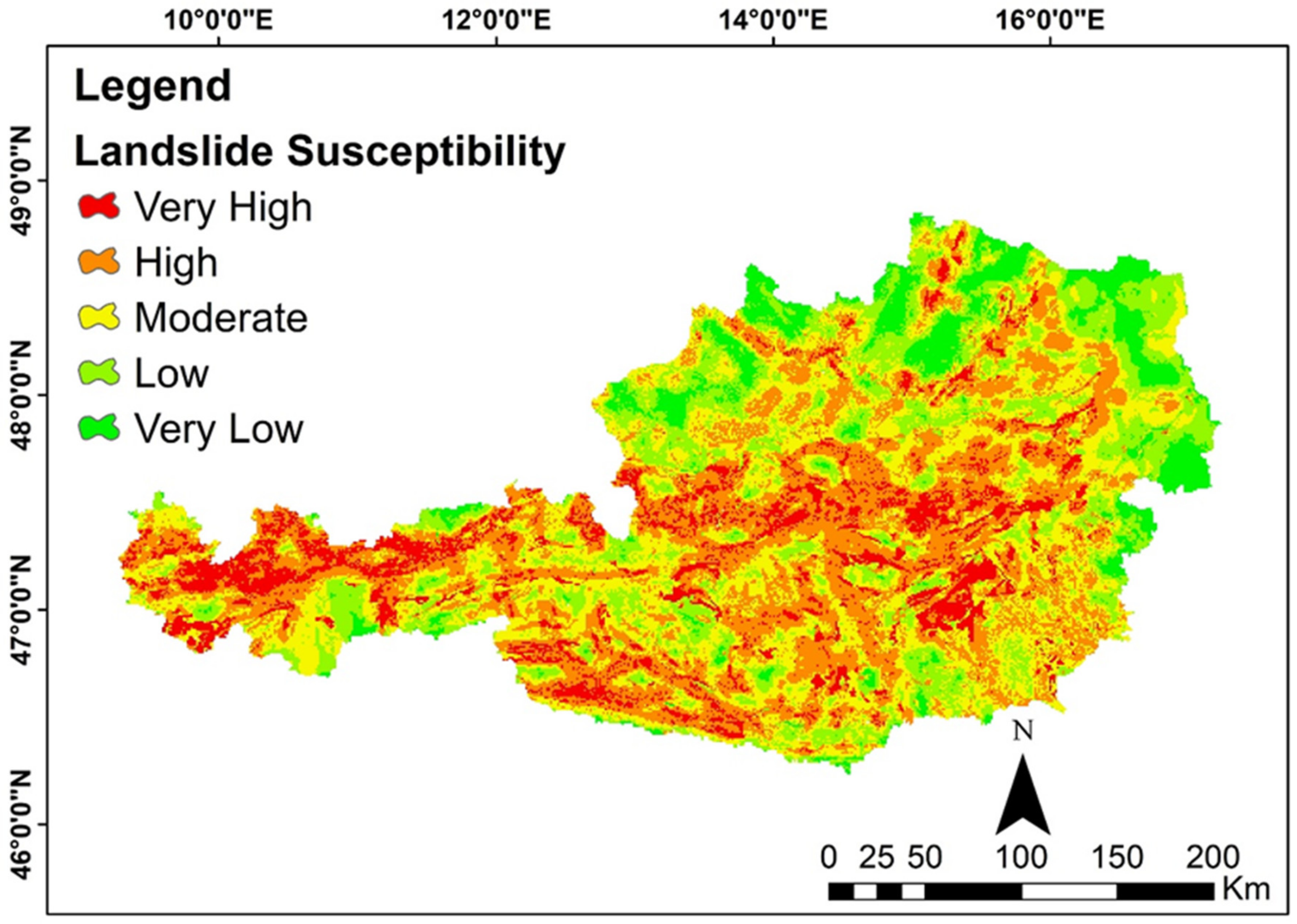
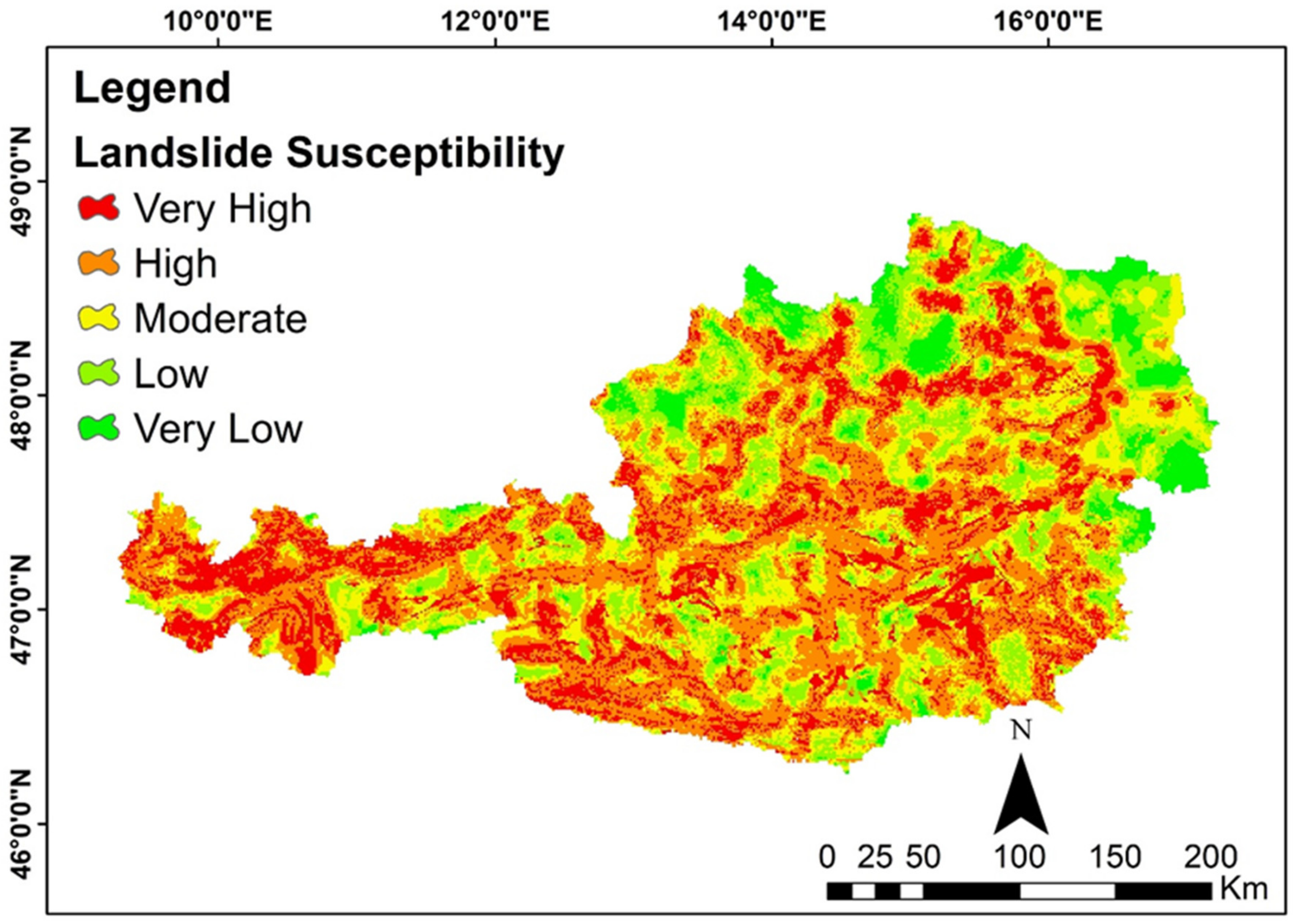
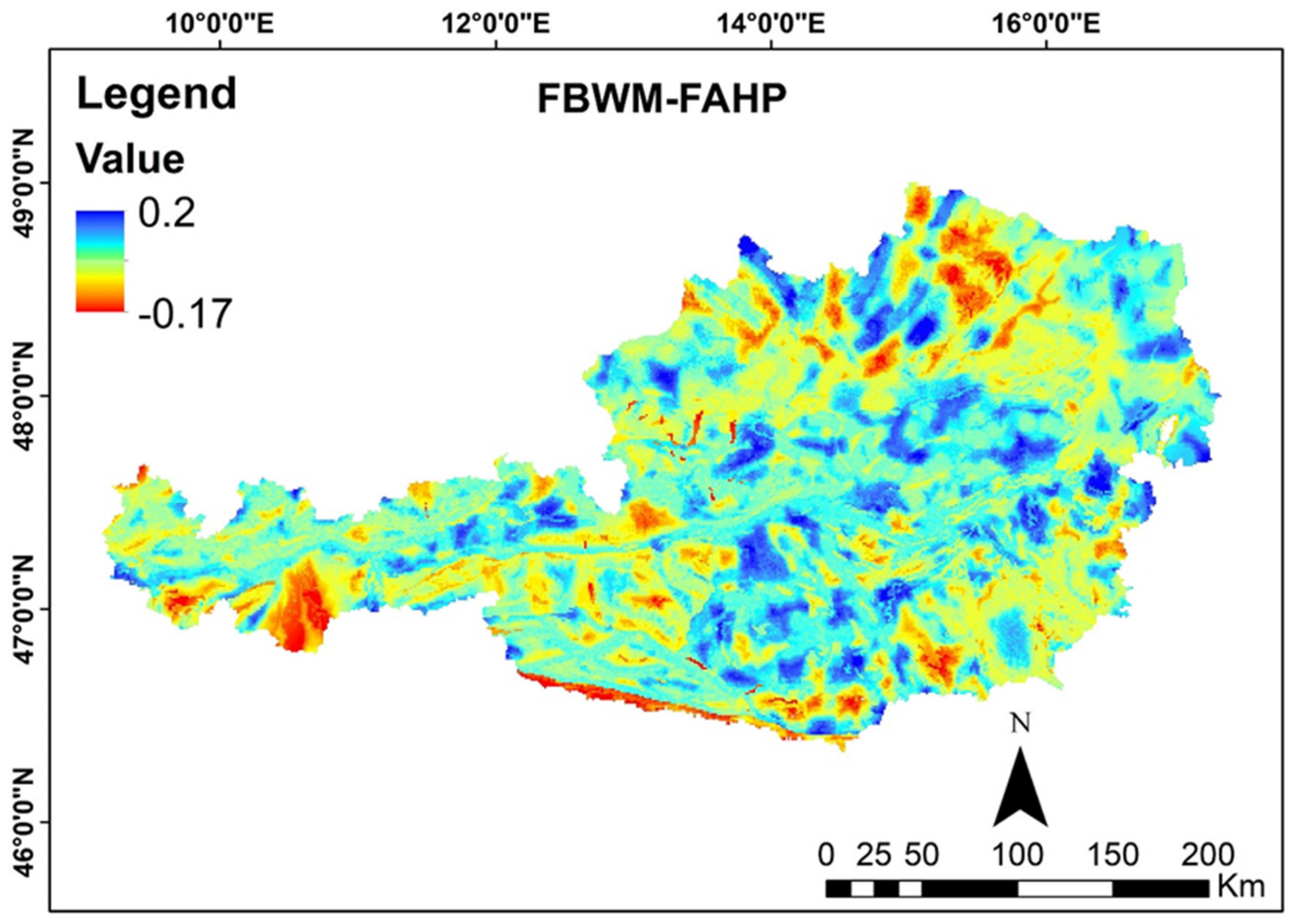
The mapping of landslide susceptible areas is for identifying areas that are prone or susceptible to future occurrences of landslides. LSM is a crucial step in the analysis of risk assessments of landslides. So far, there are very few detailed studies on landslide susceptibility mapping at a national scale in Austria. FAHP was developed for solving hierarchical problems in handling the uncertainty and vagueness that are involved in the pairwise comparison process, whereas the FBWM is an extension of classical set theory that can solve the practical problems in an uncertain environment. By comparing the approaches along with the susceptibility maps, we can concur the by the accuracy of the models regarding the suitable approach for national level landslide susceptibility mapping. For this study, we produced LSM for entire Austria based on FBWM, which is a novel approach for landslide susceptibility and also compared the results with the FAHP approach. The results clearly show that the accuracy of the FBWM approach is higher than the FAHP approach in both success rate and prediction rate curves. The AUC of the SR for the FAHP was 90% when compared to higher SR for the FBWM at 93%. Whereas, the AUC of PR for FAHP was 84% as compared to 89% for fuzzy BWM. The FBWM is a vector-based technique that needs lesser pairwise comparisons when compared to the matrix based FAHP approach. Another advantage of FBWM is that the final weights derived show higher CR when compared to MCDM approaches that do not get higher CRs.

For this study, we used the landslide inventory that was obtained from the Geological Survey of Austria that might not be yet complete and for future studies, we would like to carry out assessments with a more comprehensive landslide inventory dataset, ideally as polygons rather than points. A complementary study could be carried out based on the polygon-based landslide inventory dataset to check and compare the accuracy of the methodology and the effect of the input inventory data. This study can be further investigated with other methodologies, like machine learning and deep learning, to observe the impact of various approaches on the inventory data as well as checking the robustness of methods for this region. The resulting susceptibility map at the national scale for Austria can help planners and policymakers to better manage and plan risk mitigation measures. The resulting LSM maps can be quite useful to allocate adequate resources in regions that are more impacted by landslides.

References

1. Piralilou, S.T.; Shahabi, H.; Jarihani, B.; Ghorbanzadeh, O.; Blaschke, T.; Gholamnia, K.; Meena, S.R.; Aryal, J. Landslide detection using multi-scale image segmentation and different machine learning models in the Higher Himalayas. Remote Sens. 2019, 11, 2575. [Google Scholar] [CrossRef] [Green Version]
2. Uzielli, M.; Nadim, F.; Lacasse, S.; Kaynia, A.M. A conceptual framework for quantitative estimation of physical vulnerability to landslides. Eng. Geol. 2008, 102, 251–256. [Google Scholar] [CrossRef]
3. Petley, D. Global patterns of loss of life from landslides. Geology 2012, 40, 927–930. [Google Scholar] [CrossRef]
4. Cruden, D.M. A simple definition of a landslide. Bull. Int. Assoc. Eng. Geol. 1991, 43, 27–29. [Google Scholar] [CrossRef]
5. Reichenbach, P.; Rossi, M.; Malamud, B.D.; Mihir, M.; Guzzetti, F. A review of statistically-based landslide susceptibility models. Earth-Sci. Rev. 2018, 180, 60–91. [Google Scholar] [CrossRef]
6. Gariano, S.L.; Guzzetti, F. Landslides in a changing climate. Earth-Sci. Rev. 2016, 162, 227–252. [Google Scholar] [CrossRef] [Green Version]
7. Pourghasemi, H.R.; Rahmati, O. Prediction of the landslide susceptibility: Which algorithm, which precision? Catena 2018, 162, 177–192. [Google Scholar] [CrossRef]
8. Dou, J.; Khezri, S.; Bin Ahmad, B.; Hashim, M. Landslide susceptibility mapping at central Zab basin, Iran: A comparison between analytical hierarchy process, frequency ratio and logistic regression models. Catena 2014, 115, 55–70. [Google Scholar] [CrossRef]
9. Kim, S.; Lim, C.-H.; Kim, G.; Lee, J.; Geiger, T.; Rahmati, O.; Son, Y.; Lee, W.-K. Multi-temporal analysis of forest fire probability using socio-economic and environmental variables. Remote Sens. 2019, 11, 86. [Google Scholar] [CrossRef] [Green Version]
10. Wu, Y.; Li, W.; Wang, Q.; Liu, Q.; Yang, D.; Xing, M.; Pei, Y.; Yan, S. Landslide susceptibility assessment using frequency ratio, statistical index and certainty factor models for the Gangu County, China. Arab. J. Geosci. 2016, 9, 9. [Google Scholar] [CrossRef]
11. Hong, H.; Pradhan, B.; Xu, C.; Bui, D.T. Spatial prediction of landslide hazard at the Yihuang area (China) using two-class kernel logistic regression, alternating decision tree and support vector machines. Catena 2015, 133, 266–281. [Google Scholar] [CrossRef]
12. Roccati, A.; Faccini, F.; Luino, F.; Ciampalini, A.; Turconi, L. Heavy rainfall triggering shallow landslides: A susceptibility assessment by a GIS-approach in a Ligurian Apennine Catchment (Italy). Water 2019, 11, 605. [Google Scholar] [CrossRef] [Green Version]
13. Roodposhti, M.S.; Aryal, J.; Pradhan, B. A novel rule-based approach in mapping landslide susceptibility. Sensors 2019, 19, 2274. [Google Scholar] [CrossRef] [PubMed] [Green Version]
14. Van Westen, C. Remote sensing and GIS for natural hazards assessment and disaster risk management. In Treatise on Geomorphology; Academic Press: San Diego, CA, USA, 2013; Volume 3, pp. 259–298. [Google Scholar]
15. Petschko, H.; Brenning, A.; Bell, R.; Goetz, J.; Glade, T. Assessing the quality of landslide susceptibility maps—Case study Lower Austria. Nat. Hazards Earth Syst. Sci. 2014, 14, 95–118. [Google Scholar] [CrossRef] [Green Version]
16. Kanungo, D.P.; Arora, M.; Sarkar, S.; Gupta, R. A comparative study of conventional, ANN black box, fuzzy and combined neural and fuzzy weighting procedures for landslide susceptibility zonation in Darjeeling Himalayas. Eng. Geol. 2006, 85, 347–366. [Google Scholar] [CrossRef]
17. Abdollahi, S.; Pourghasemi, H.R.; Ghanbarian, G.; Safaeian, R. Prioritization of effective factors in the occurrence of land subsidence and its susceptibility mapping using an SVM model and their different kernel functions. Bull. Int. Assoc. Eng. Geol. 2018, 78, 4017–4034. [Google Scholar] [CrossRef]
18. Chen, W.; Chen, W.; Panahi, M.; Kornejady, A.; Wang, J.; Xie, X.; Cao, S. Spatial prediction of landslide susceptibility using an adaptive neuro-fuzzy inference system combined with frequency ratio, generalized additive model, and support vector machine techniques. Geomorphology 2017, 297, 69–85. [Google Scholar] [CrossRef]
19. Panahi, M.; Sadhasivam, N.; Pourghasemi, H.R.; Rezaie, F.; Lee, S. Spatial prediction of groundwater potential mapping based on convolutional neural network (CNN) and support vector regression (SVR). J. Hydrol. 2020, 588, 125033. [Google Scholar] [CrossRef]
20. Ghorbanzadeh, O.; Blaschke, T.; Aryal, J.; Gholaminia, K. A new GIS-based technique using an adaptive neuro-fuzzy inference system for land subsidence susceptibility mapping. J. Spat. Sci. 2018, 1–17. [Google Scholar] [CrossRef] [Green Version]
21. Arabameri, A.; Pradhan, B.; Rezaei, K.; Conoscenti, C. Gully erosion susceptibility mapping using GIS-based multi-criteria decision analysis techniques. Catena 2019, 180, 282–297. [Google Scholar] [CrossRef]
22. Pourghasemi, H.R.; Beheshtirad, M.; Pradhan, B. A comparative assessment of prediction capabilities of modified analytical hierarchy process (M-AHP) and Mamdani fuzzy logic models using Netcad-GIS for forest fire susceptibility mapping. Geomat. Nat. Hazards Risk 2014, 7, 1–25. [Google Scholar] [CrossRef] [Green Version]
23. Naboureh, A.; Feizizadeh, B.; Bian, J.; Blaschke, T.; Ghorbanzadeh, O.; Moharrami, M. Traffic accident spatial simulation modeling for planning of road emergency services. ISPRS Int. J. Geo-Inf. 2019, 8, 371. [Google Scholar] [CrossRef] [Green Version]
24. Martín, J.C.; Román, C.; Viñán, C. An Institutional Trust Indicator Based on Fuzzy Logic and Ideal Solutions. Mathematics 2020, 8, 807. [Google Scholar] [CrossRef]
25. Jin, H.; Zhang, M.; Yuan, Y. Analytic network process-based multi-criteria decision approach and sensitivity analysis for temporary facility layout planning in construction projects. Appl. Sci. 2018, 8, 2434. [Google Scholar] [CrossRef] [Green Version]
26. Kavurmacı, M.; Karakuş, C.B. Evaluation of irrigation water quality by data envelopment analysis and analytic hierarchy process-based water quality indices: The case of Aksaray City, Turkey. Water Air Soil Pollut. 2020, 231, 55. [Google Scholar] [CrossRef]
27. De Brito, M.M.; Almoradie, A.; Evers, M. Spatially-explicit sensitivity and uncertainty analysis in a MCDA-based flood vulnerability model. Int. J. Geogr. Inf. Sci. 2019, 33, 1788–1806. [Google Scholar] [CrossRef]
28. Maqsoom, A.; Aslam, B.; Khalil, U.; Ghorbanzadeh, O.; Ashraf, H.; Faisal Tufail, R.; Farooq, D.; Blaschke, T. A GIS-based DRASTIC Model and an Adjusted DRASTIC Model (DRASTICA) for Groundwater Susceptibility Assessment along the China–Pakistan Economic Corridor (CPEC) Route. ISPRS Int. J. Geo-Inf. 2020, 9, 332. [Google Scholar] [CrossRef]
29. Moslem, S.; Ghorbanzadeh, O.; Blaschke, T.; Duleba, S. Analysing stakeholder consensus for a sustainable transport development decision by the fuzzy AHP and interval AHP. Sustainability 2019, 11, 3271. [Google Scholar] [CrossRef] [Green Version]
30. Rezaei, J. Best-worst multi-criteria decision-making method. Omega 2015, 53, 49–57. [Google Scholar] [CrossRef]
31. Gigovic, L.; Drobnjak, S.; Pamučar, D. The application of the hybrid GIS spatial multi-criteria decision analysis best–worst methodology for landslide susceptibility mapping. ISPRS Int. J. Geo-Inf. 2019, 8, 79. [Google Scholar] [CrossRef] [Green Version]
32. Tasser, E.; Mader, M.; Tappeiner, U. Effects of land use in alpine grasslands on the probability of landslides. Basic Appl. Ecol. 2003, 4, 271–280. [Google Scholar] [CrossRef]
33. Balteanu, D.; Chendes, V.; Sima, M.; Enciu, P. A country-wide spatial assessment of landslide susceptibility in Romania. Geomorphology 2010, 124, 102–112. [Google Scholar] [CrossRef]
34. Trigila, A.; Frattini, P.; Casagli, N.; Catani, F.; Crosta, G.; Esposito, C.; Iadanza, C.; Lagomarsino, D.; Mugnozza, G.S.; Segoni, S.; et al. Landslide susceptibility mapping at national scale: The Italian case study. Landslide Sci. Pract. 2013, 287–295. [Google Scholar] [CrossRef] [Green Version]
35. Suh, J.; Choi, Y.; Roh, T.-D.; Lee, H.-J.; Park, H.-D. National-scale assessment of landslide susceptibility to rank the vulnerability to failure of rock-cut slopes along expressways in Korea. Environ. Earth Sci. 2010, 63, 619–632. [Google Scholar] [CrossRef]
36. Malet, J.; Puissant, A.; Mathieu, A.; Eeckhaut, M.V.D.; Fressard, M.; Margottini, C.; Canuti, P.; Sassa, K. Integrating spatial multi-criteria evaluation and expert knowledge for country-scale landslide susceptibility analysis: Application to France. In Landslide Science and Practice; Springer: Berlin/Heidelberg, Germany, 2013; pp. 303–311. [Google Scholar]
37. Ferentinou, M.; Chalkias, C. Mapping mass movement susceptibility across Greece with GIS, ANN and statistical methods. In Landslide Science and Practice; Springer: Berlin/Heidelberg, Germany, 2013; pp. 321–327. [Google Scholar]
38. Nachappa, T.G.; Piralilou, S.T.; Ghorbanzadeh, O.; Shahabi, H.; Blaschke, T. Landslide susceptibility mapping for Austria Using Geons and optimization with the Dempster–Schafer theory. Appl. Sci. 2019, 9, 5393. [Google Scholar] [CrossRef] [Green Version]
39. Lima, P.H.; Steger, S.; Glade, T.; Tilch, N.; Schwarz, L.; Kociu, A.; Mikoš, M.; Tiwari, B.; Yin, Y.; Sassa, K.; et al. Landslide susceptibility mapping at national scale: A first attempt for Austria. In Proceedings of the World Landslide Forum, Ljubljana, Slovenia, 29 May–2 June 2017; pp. 943–951. [Google Scholar]
40. Glade, T.; Petschko, H.; Bell, R.; Bauer, C.; Granica, K.; Heiss, G.; Leopold, P.; Pomaroli, G.; Proske, H.; Schweigl, J.; et al. Landslide Susceptibility Maps for Lower Austria—Methods and Challenges; Koboltschnig, G., Hübl, J., Braun, J., Eds.; International Research Society INTERPRAEVENT: Grenoble, France, 2012; Volume 1, pp. 497–508. [Google Scholar]
41. Embletion-Hamann, C. Geomorphological hazards in Austria. In Geomorphology for the Future; Kellerer-Pirklbauer, A., Keiler, M., Embleton-Hamann, C., Stötter, J., Eds.; Innsbruck University Press: Innsbruck, Austria, 2007; ISBN 978-3-902571-18-2. [Google Scholar]
42. Guzzetti, F.; Mondini, A.C.; Cardinali, M.; Fiorucci, F.; Santangelo, M.; Chang, K.-T. Landslide inventory maps: New tools for an old problem. Earth-Sci. Rev. 2012, 112, 42–66. [Google Scholar] [CrossRef] [Green Version]
43. Ayalew, L.; Yamagishi, H. The application of GIS-based logistic regression for landslide susceptibility mapping in the Kakuda-Yahiko Mountains, Central Japan. Geomorphology 2005, 65, 15–31. [Google Scholar] [CrossRef]
44. Mahdadi, F.; Boumezbeur, A.; Hadji, R.; Kanungo, D.P.; Zahri, F. GIS-based landslide susceptibility assessment using statistical models: A case study from Souk Ahras province, N-E Algeria. Arab. J. Geosci. 2018, 11, 476. [Google Scholar] [CrossRef]
45. Conoscenti, C.; Rotigliano, E.; Cama, M.; Arias, N.A.C.; Lombardo, L.; Agnesi, V. Exploring the effect of absence selection on landslide susceptibility models: A case study in Sicily, Italy. Geomorphology 2016, 261, 222–235. [Google Scholar] [CrossRef]
46. Ghorbanzadeh, O.; Blaschke, T.; Gholamnia, K.; Meena, S.R.; Tiede, D.; Aryal, J. Evaluation of different machine learning methods and deep-learning convolutional neural networks for landslide detection. Remote Sens. 2019, 11, 196. [Google Scholar] [CrossRef] [Green Version]
47. Pham, B.T.; Prakash, I.; Khosravi, K.; Chapi, K.; Trinh, P.T.; Ngo, T.Q.; Hosseini, S.V.; Bui, D.T. A comparison of support vector machines and Bayesian algorithms for landslide susceptibility modelling. Geocarto Int. 2018, 34, 1385–1407. [Google Scholar] [CrossRef]
48. Pourghasemi, H.R.; Gayen, A.; Park, S.-J.; Lee, C.W.; Lee, S. Assessment of landslide-prone areas and their zonation using logistic regression, LogitBoost, and NaïveBayes machine-learning algorithms. Sustainability 2018, 10, 3697. [Google Scholar] [CrossRef] [Green Version]
49. Harris, S.M.; Carvalho, L.V. Atmospheric River Development and Effects on Southern California; American Geophysical Union: Washington, DC, USA, 2014. [Google Scholar]
50. Tsangaratos, P.; Ilia, I. Landslide susceptibility mapping using a modified decision tree classifier in the Xanthi Perfection, Greece. Landslides 2015, 13, 305–320. [Google Scholar] [CrossRef]
51. Yan, G.; Liang, S.; Gui, X.; Xie, Y.; Zhao, H. Optimizing landslide susceptibility mapping in the Kongtong District, NW China: Comparing the subdivision criteria of factors. Geocarto Int. 2018, 34, 1408–1426. [Google Scholar] [CrossRef]
52. Yalcin, A.; Bulut, F. Landslide susceptibility mapping using GIS and digital photogrammetric techniques: A case study from Ardesen (NE-Turkey). Nat. Hazards 2006, 41, 201–226. [Google Scholar] [CrossRef]
53. Segoni, S.; Pappafico, G.; Luti, T.; Catani, F. Landslide susceptibility assessment in complex geological settings: Sensitivity to geological information and insights on its parameterization. Landslides 2020, 1–11. [Google Scholar] [CrossRef] [Green Version]
54. Meneses, B.; Pereira, S.; Reis, E. Effects of different land use and land cover data on the landslide susceptibility zonation of road networks. Nat. Hazards Earth Syst. Sci. 2019, 19, 471–487. [Google Scholar] [CrossRef] [Green Version]
55. Bui, D.T.; Pradhan, B.; Löfman, O.; Revhaug, I. Regional prediction of landslide hazard using probability analysis of intense rainfall in the Hoa Binh province, Vietnam. Nat. Hazards 2012, 66, 707–730. [Google Scholar] [CrossRef]
56. Moslem, S.; Duleba, S. Application of AHP for evaluating passenger demand for public transport improvements in Mersin, Turkey. Pollack Period. 2018, 13, 67–76. [Google Scholar] [CrossRef]
57. Ghorbanzadeh, O.; Moslem, S.; Blaschke, T.; Duleba, S. Sustainable urban transport planning considering different stakeholder groups by an interval-AHP decision support model. Sustainability 2018, 11, 9. [Google Scholar] [CrossRef] [Green Version]
58. Moslem, S.; Farooq, D.; Ghorbanzadeh, O.; Blaschke, T. Application of the AHP-BWM Model for evaluating driver behavior factors related to road safety: A case study for Budapest. Symmetry 2020, 12, 243. [Google Scholar] [CrossRef] [Green Version]
59. Wang, Y.-M.; Chin, K.-S. Fuzzy analytic hierarchy process: A logarithmic fuzzy preference programming methodology. Int. J. Approx. Reason. 2011, 52, 541–553. [Google Scholar] [CrossRef] [Green Version]
60. Farooq, D.; Moslem, S.; Tufail, R.F.; Ghorbanzadeh, O.; Duleba, S.; Maqsoom, A.; Blaschke, T. Analyzing the importance of driver behavior criteria related to road safety for different driving cultures. Int. J. Environ. Res. Public Health 2020, 17, 1893. [Google Scholar] [CrossRef] [PubMed] [Green Version]
61. Cheng, C.-H. Evaluating naval tactical missile systems by fuzzy AHP based on the grade value of membership function. Eur. J. Oper. Res. 1997, 96, 343–350. [Google Scholar] [CrossRef]
62. Van Laarhoven, P.J.; Pedrycz, W. A fuzzy extension of Saaty’s priority theory. Fuzzy Sets Syst. 1983, 11, 229–241. [Google Scholar] [CrossRef]
63. Rossi, M.; Guzzetti, F.; Reichenbach, P.; Mondini, A.C.; Peruccacci, S. Optimal landslide susceptibility zonation based on multiple forecasts. Geomorphology 2010, 114, 129–142. [Google Scholar] [CrossRef]
64. Ghorbanzadeh, O.; Rostamzadeh, H.; Blaschke, T.; Gholaminia, K.; Aryal, J. A new GIS-based data mining technique using an adaptive neuro-fuzzy inference system (ANFIS) and k-fold cross-validation approach for land subsidence susceptibility mapping. Nat. Hazards 2018, 94, 497–517. [Google Scholar] [CrossRef] [Green Version]
65. Linden, A. Measuring diagnostic and predictive accuracy in disease management: An introduction to receiver operating characteristic (ROC) analysis. J. Eval. Clin. Pr. 2006, 12, 132–139. [Google Scholar] [CrossRef]
66. Baird, C.; Healy, T.; Johnson, K.; Bogie, A.; Dankert, E.W.; Scharenbroch, C. A Comparison of Risk Assessment Instruments in Juvenile Justice; National Council on Crime and Delinquency: Madison, WI, USA, 2013. [Google Scholar]
67. Gigovic, L.; Pamucar, D.; Božanić, D.; Ljubojevic, S. Application of the GIS-DANP-MABAC multi-criteria model for selecting the location of wind farms: A case study of Vojvodina, Serbia. Renew. Energy 2017, 103, 501–521. [Google Scholar] [CrossRef]
68. Farooq, D.; Moslem, S. A fuzzy dynamical approach for examining driver behavior criteria related to road safety. In Proceedings of the 2019 Smart City Symposium Prague (SCSP), Prague, Czech Republic, 23–24 May 2019; pp. 1–7. [Google Scholar]
Figure 1. The study area.
Ijgi 09 00393 g001
Figure 2. The triangular fuzzy set.
Ijgi 09 00393 g002
Figure 3. The proposed methodology for Fuzzy Analytical hierarchical process (FAHP).
Ijgi 09 00393 g003
Figure 4. Land susceptibility map for Austria using the FBWM model.
Ijgi 09 00393 g004
Figure 5. Land susceptibility map for Austria using FAHP model.
Ijgi 09 00393 g005
Figure 6. Success Rate (SR) and Prediction Rate (PR) curves for the FAHP and FBWM models. (a). SR- area under the curve (SR-AUC) for the FAHP; (b). SR-AUC for FBWM; (c). PR-AUC for the FAHP; and, (d). PR-AUC for FBWM.
Ijgi 09 00393 g006
Figure 7. Comparison of FBWM-FAHP.
Ijgi 09 00393 g007
Figure 8. Spatial location of overestimations, in relationship with the imbalanced classes.
Ijgi 09 00393 g008
Figure 9. Spatial location of underestimations, in relationship with the imbalanced classes.
Ijgi 09 00393 g009