Measuring Accessibility of Healthcare Facilities for Populations with Multiple Transportation Modes Considering Residential Transportation Mode Choice


Abstract
:1. Introduction
2. Materials and Methods
2.1. Review of the Traditional Generalized 2SFCA Model
2.2. Review of the Traditional STM G2SFCA Model
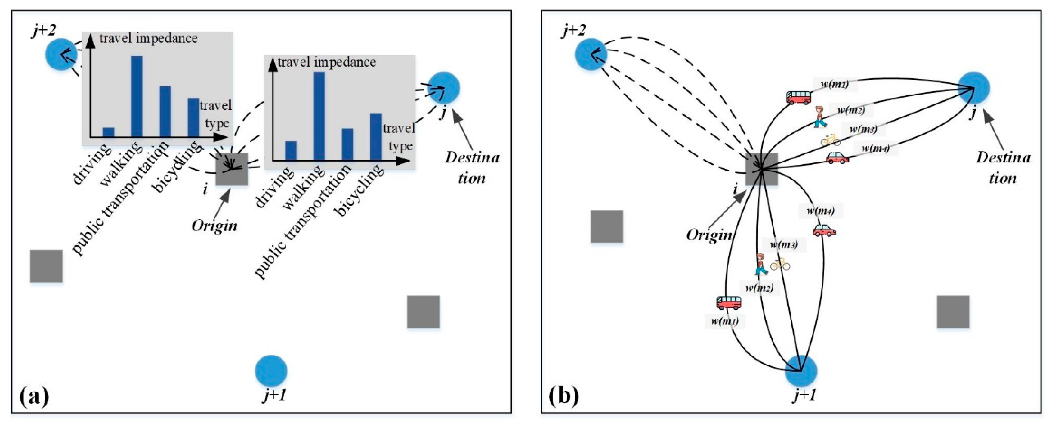
2.3. Designing the MTM G2SFCA Model
2.4. Designing the MTM-RTMC G2SFCA Model
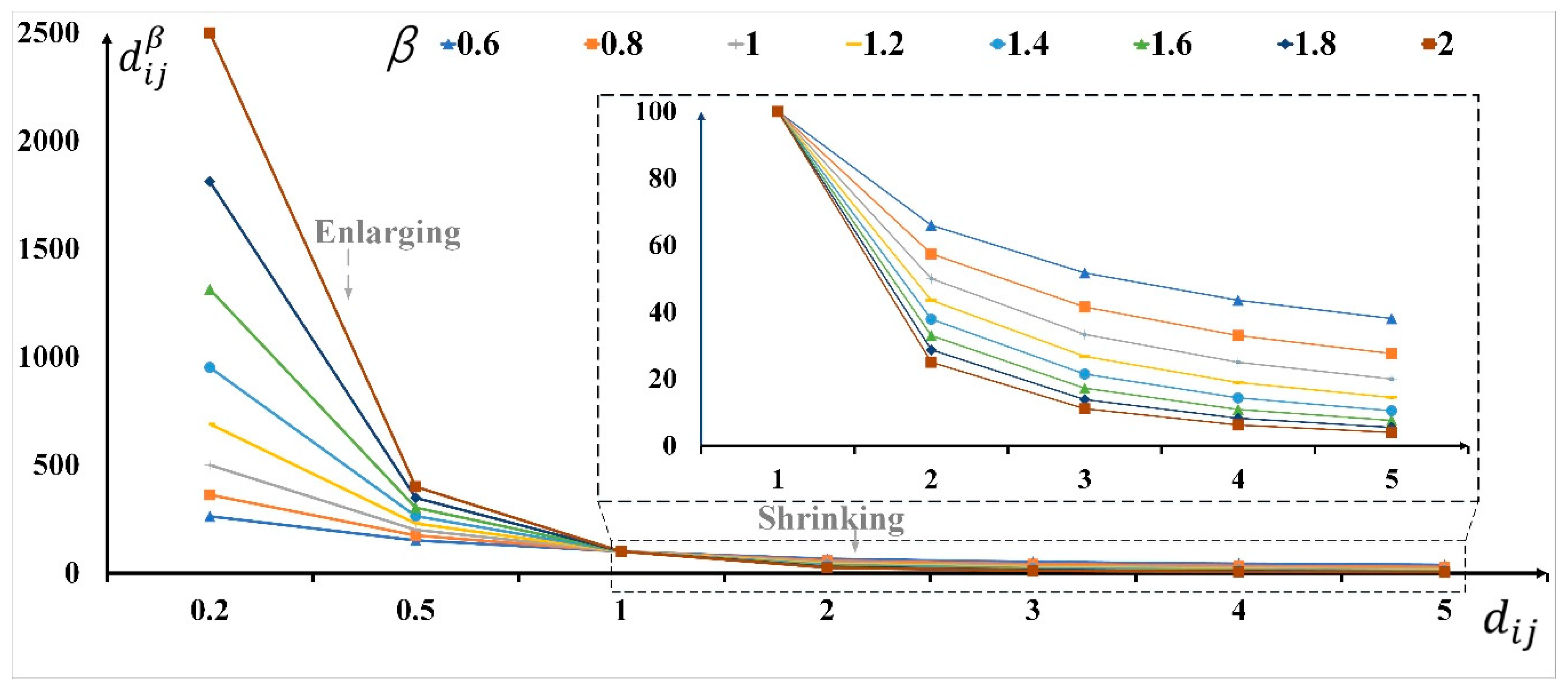
2.5. Travel Friction Coefficient β
- (1)
- In short-distance travel, the travel times of the four main transportation modes are similar. The residents tend to adopt low-cost transportation modes, such as walking or cycling, so the travel speed and the travel friction coefficient β have a negative correlation. In short-distance travel, the travel friction coefficient β in the high-speed transportation mode offers a relatively smaller enhancement of the travel impedance as the speed of the transportation mode increases. So, the travel friction coefficient β in the high-speed transportation mode is relatively low.
- (2)
- For long-distance travel, the travel time of the four main transportation modes varies greatly. The diversity of alternative transportation modes gradually decreases, and residents tend to choose faster transportation modes, which can ensure shorter transit times. As the speed of the transportation mode increases, the travel friction coefficient β of the high-speed transportation mode has a relatively smaller effect on suppressing the travel impedance, so the travel friction coefficient β of the high-speed transportation mode is relatively low.
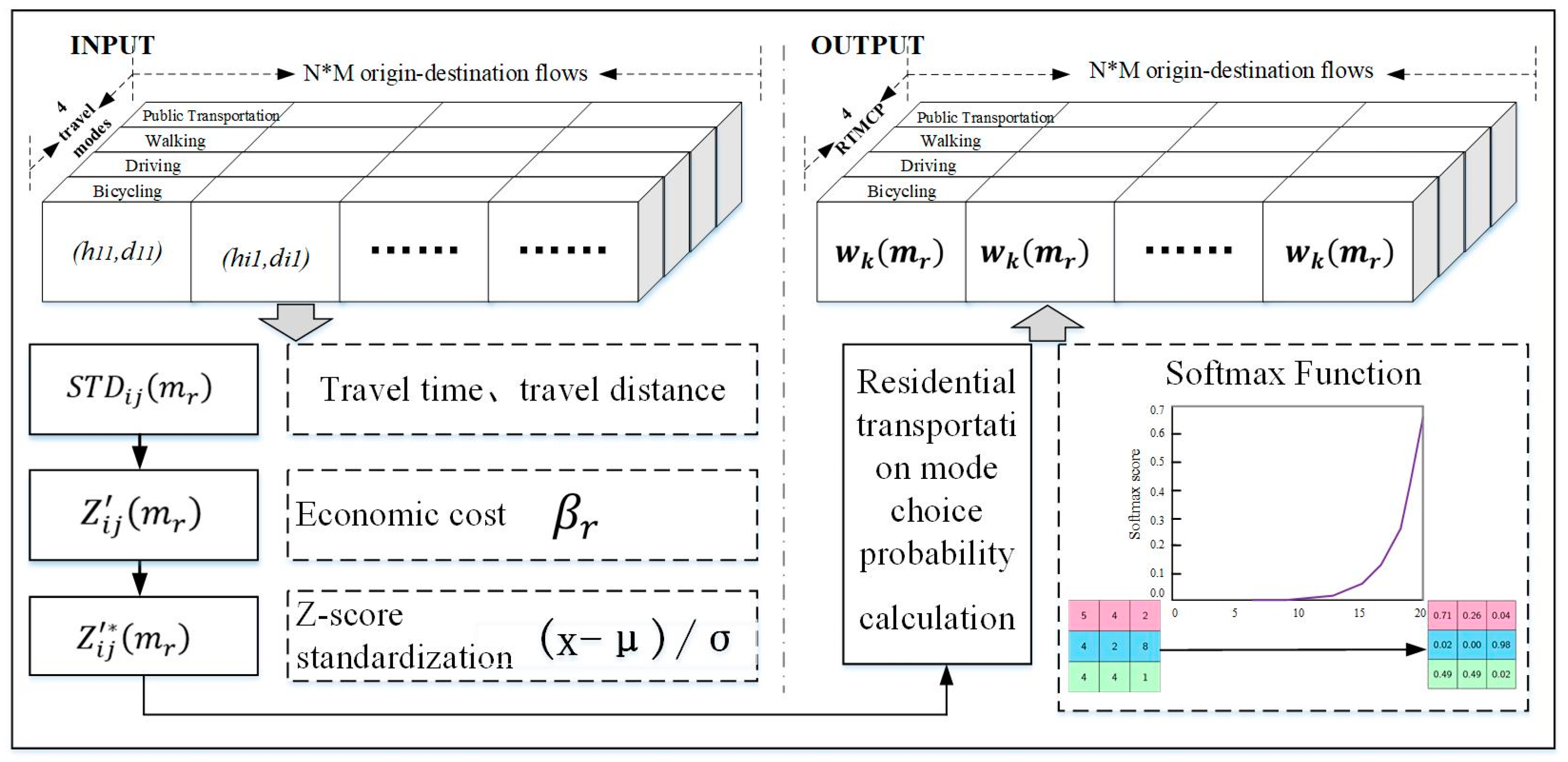
2.6. Residential Transportation Mode Choice Probabilities wk(mr)
3. Study Area and Data
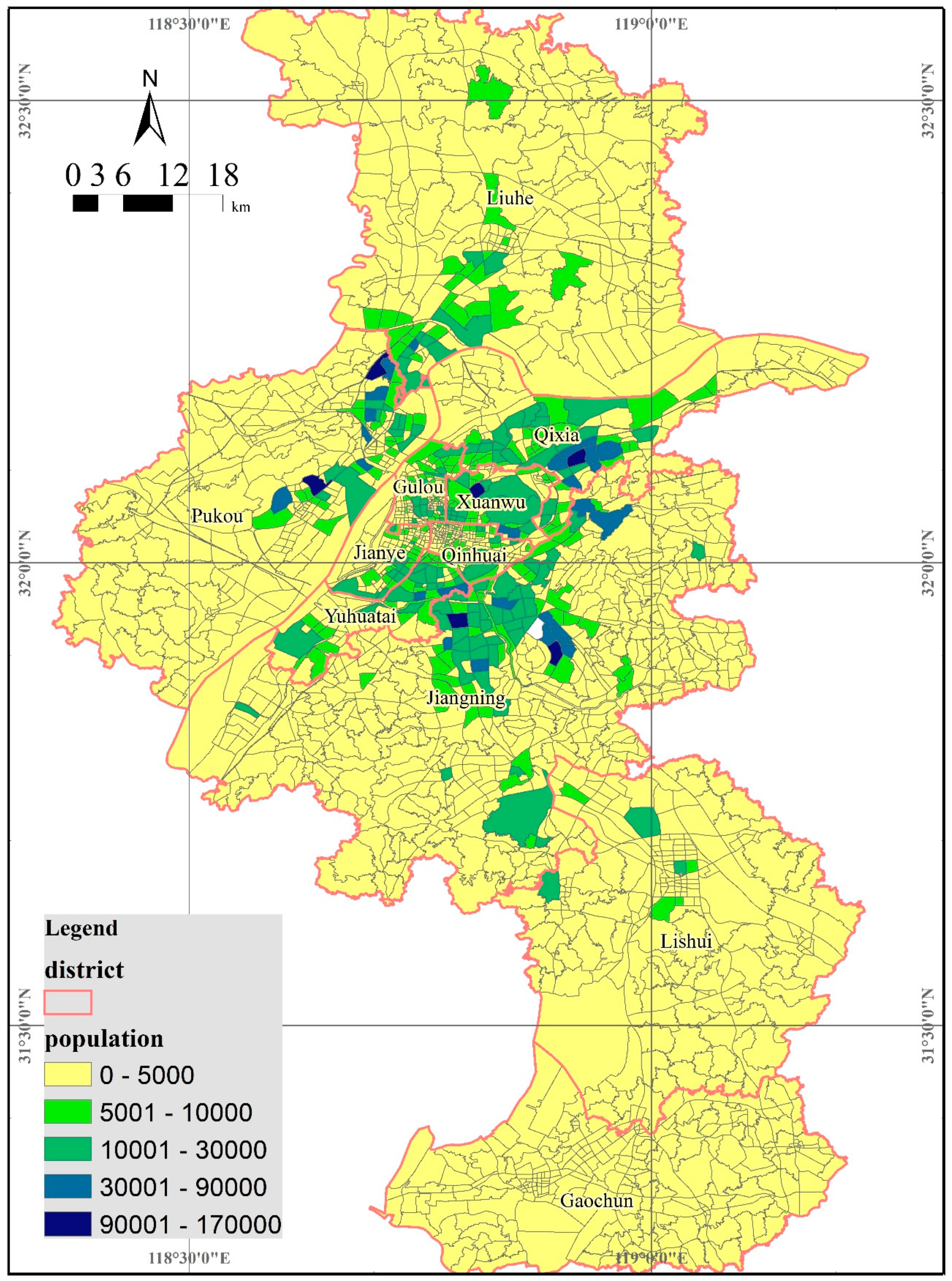
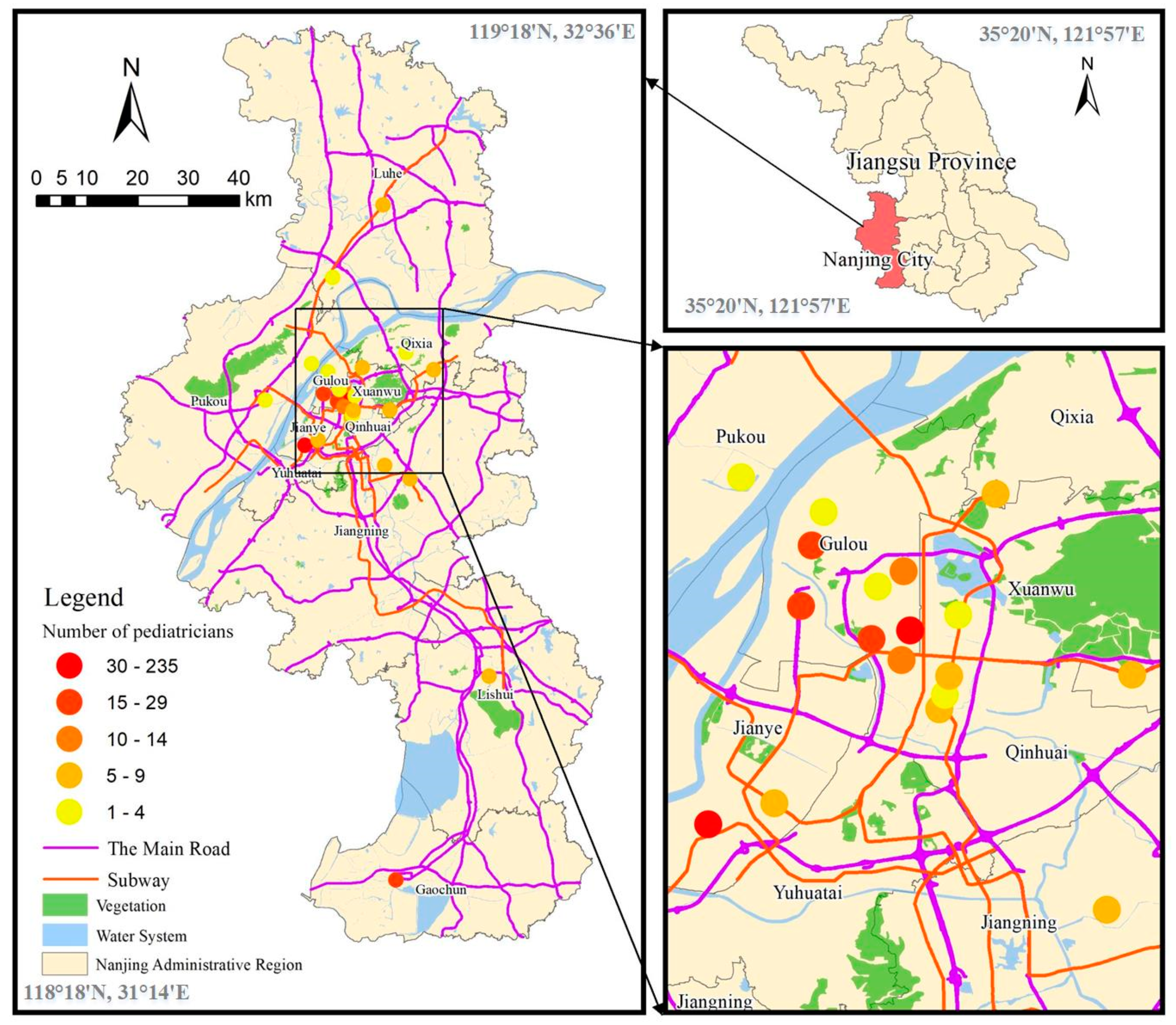
3.1. Study Area
3.2. Data
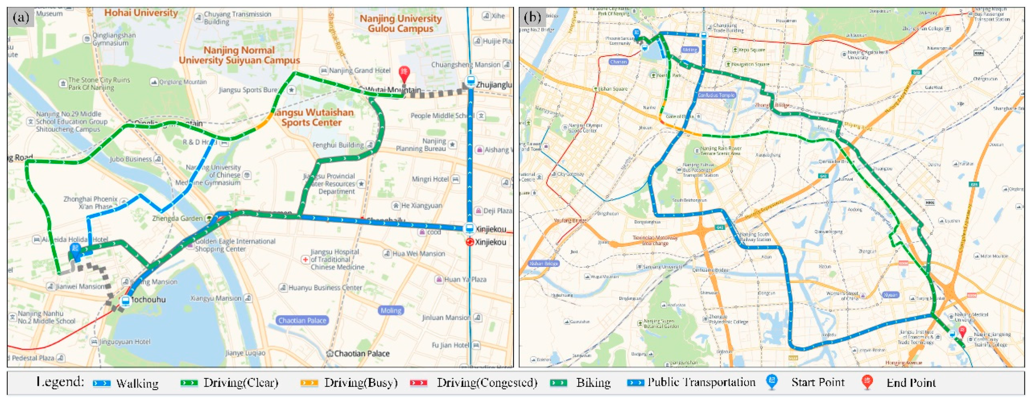
3.2.1. Route Planning Data of Multiple Transportation Modes
3.2.2. Child Population Spatial Distribution Data
3.2.3. Pediatric Clinic Services Data
3.3. Ethical Consideration
4. Results
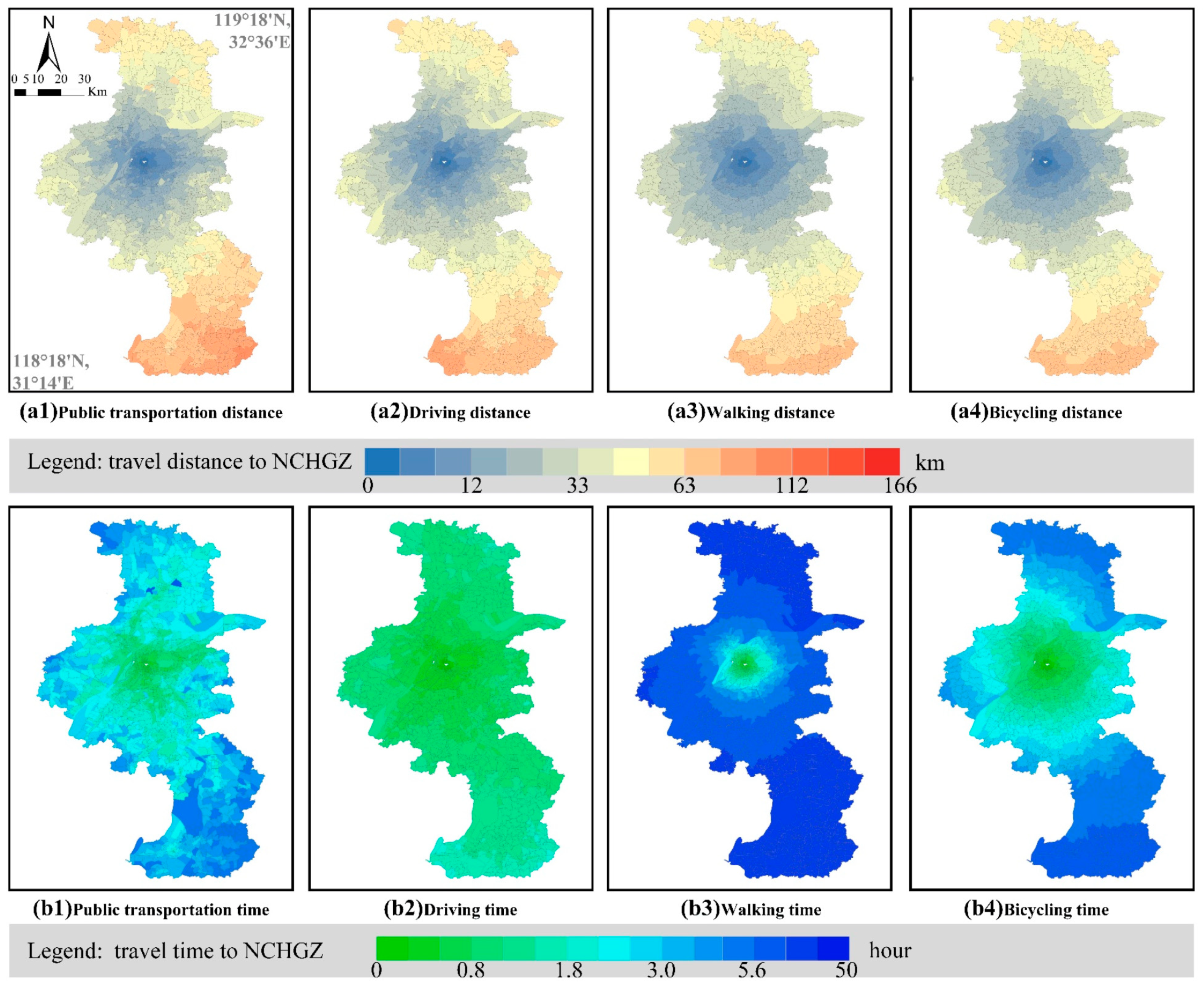
4.1. dij Establishment
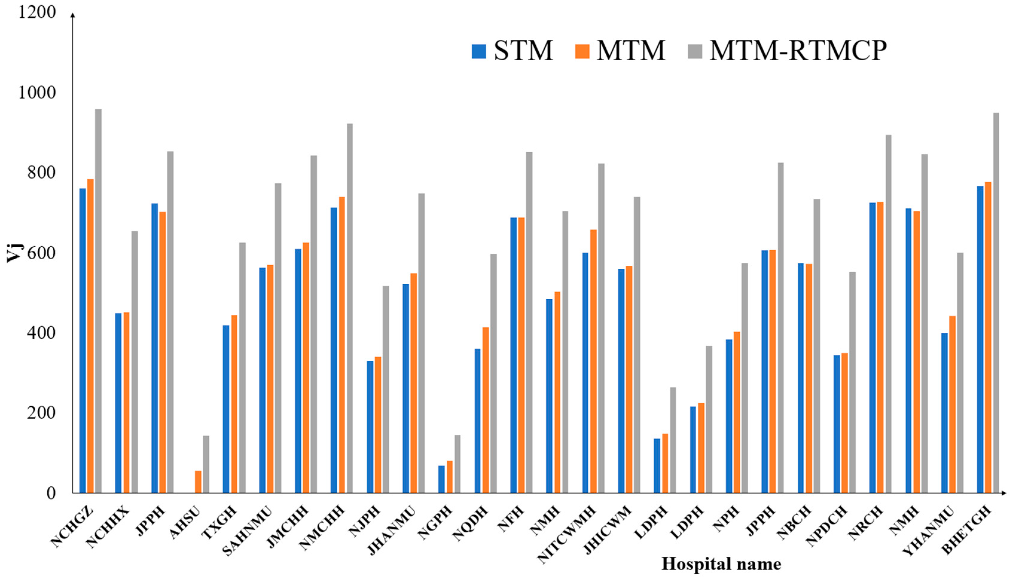
4.2. Comparison of the Vij Estimates with the Three G2SFCA Models
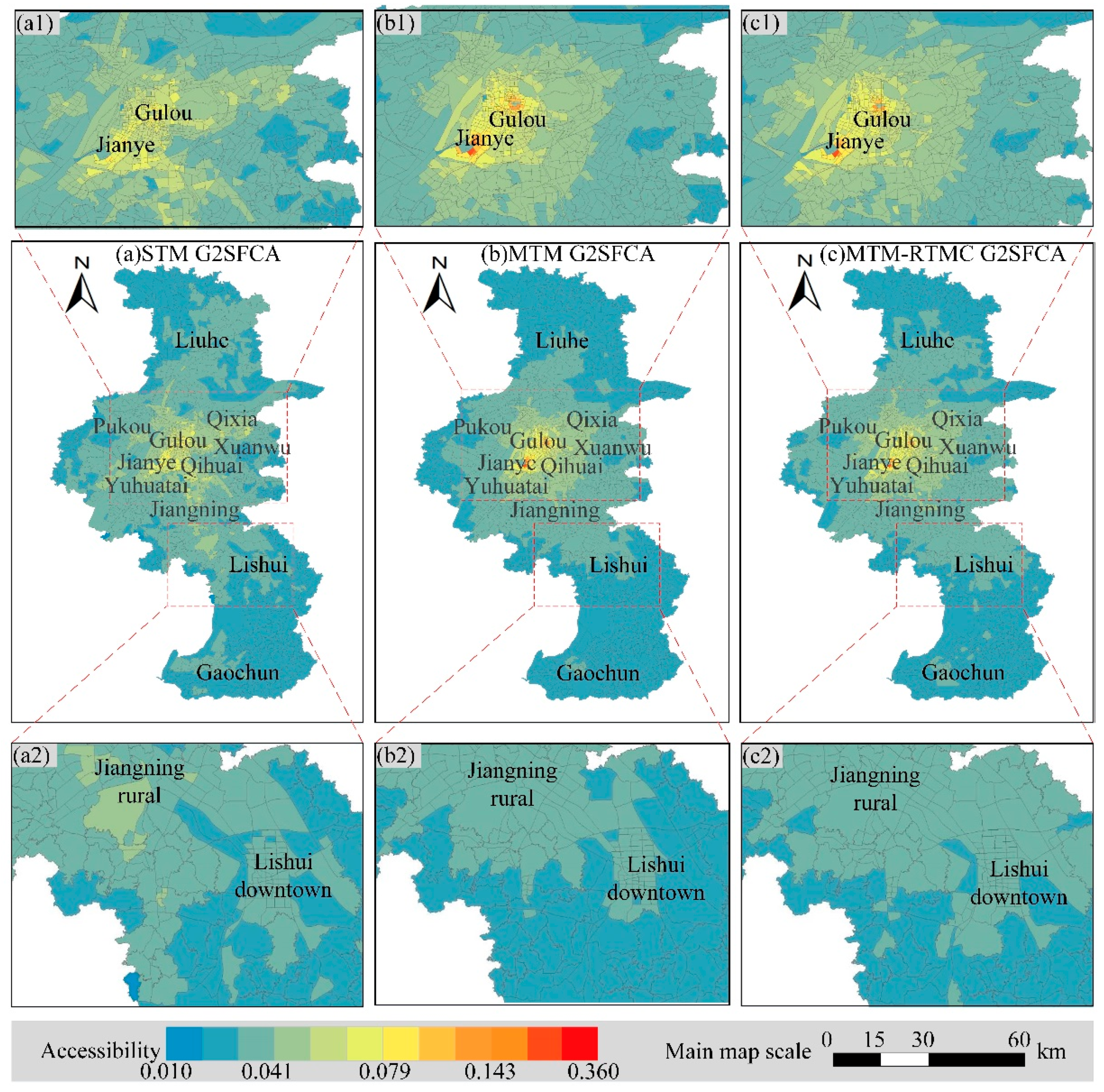
4.3. Comparison of the Accessibility Estimates from the Three G2SFCA Models
5. Discussion
5.1. The Potential Application of This MTM-RTCM Mechanism
5.2. Implications and Theoretical Thinking of the Proposed Method
6. Conclusions
Supplementary Materials
Author Contributions
Funding
Acknowledgments
Conflicts of Interest
Appendix A

| ID | Hospital Name | Abbreviation | Longitude | Latitude | Number of Pediatricians | Hospital Level |
|---|---|---|---|---|---|---|
| 1 | Nanjing Children’s Hospital Guangzhou Road Office | NCHGZ | 118.7742 | 32.0527 | 157 | 3 |
| 2 | Nanjing Children’s Hospital Hexi Office | NCHHX | 118.7026 | 31.9840 | 235 | 3 |
| 3 | Jiangsu Provincial People’s Hospital | JPPH | 118.7600 | 32.0500 | 26 | 3 |
| 4 | Affiliated Hospital of Southeast University | AHSU | 118.7720 | 32.7020 | 13 | 3 |
| 5 | Taikang Xianlin Gulou Hospital | TXGH | 118.9330 | 32.0950 | 6 | 3 |
| 6 | Second Affiliated Hospital of Nanjing Medical University | SAHNMU | 118.7390 | 32.0810 | 26 | 3 |
| 7 | Jiangsu Maternal and Child Healthcare Hospital | JMCHH | 118.7360 | 32.0600 | 23 | 3 |
| 8 | Nanjing Maternal and Child Healthcare Hospital | NMCHH | 118.7710 | 32.0410 | 14 | 3 |
| 9 | Nanjing Jiangbei People’s Hospital | NJPH | 118.7520 | 32.2370 | 3 | 3 |
| 10 | Jiangning Hospital affiliated to Nanjing Medical University | JHANMU | 118.8440 | 31.9500 | 8 | 3 |
| 11 | Nanjing Gaochun People’s Hospital | NGPH | 118.8650 | 31.3220 | 20 | 2 |
| 12 | Nanjing Qixia District Hospital | NQDH | 118.8820 | 32.1220 | 2 | 2 |
| 13 | Nanjing First Hospital | NFH | 118.7870 | 32.0220 | 8 | 3 |
| 14 | Nanjing Mingji Hospital | NMH | 118.7200 | 31.9810 | 6 | 3 |
| 15 | Nanjing Integrated Traditional Chinese and Western Medicine Hospital | NITCWMH | 118.8530 | 32.0350 | 9 | 3 |
| 16 | Jiangsu Hospital of Integrated Chinese and Western Medicine | JHICWM | 118.8040 | 32.0990 | 6 | 3 |
| 17 | Lishui District People’s Hospital | LDPH | 119.0270 | 31.6320 | 6 | 3 |
| 18 | Liuhe District People’s Hospital | LDPH | 118.8400 | 32.3420 | 9 | 2 |
| 19 | Nanjing Pukou Hospital | NPH | 118.7140 | 32.1060 | 4 | 2 |
| 20 | Jiangsu Province Provincial Hospital | JPPH | 118.7360 | 32.0670 | 2 | 3 |
| 21 | Nanjing Branch of Changzheng Hospital | NBCH | 118.7440 | 32.0930 | 1 | 3 |
| 22 | Nanjing Pukou District Central Hospital | NPDCH | 118.6320 | 32.0500 | 3 | 2 |
| 23 | Nanjing Red Cross Hospital | NRCH | 118.7870 | 32.0280 | 1 | 2 |
| 24 | Nanjing Municipal Hospital | NMH | 118.7890 | 32.0560 | 1 | 2 |
| 25 | Yifu Hospital Affiliated to Nanjing Medical University | YHANMU | 118.8880 | 31.9330 | 8 | 3 |
| 26 | Bayi Hospital of Eastern Theater General Hospital | BHETGH | 118.7880 | 32.0360 | 6 | 3 |
References
- Jin, Z.; Northridge, M.E.; Metcalf, S.S. Modeling the influence of social ties and transportation choice on access to oral healthcare for older adults. Appl. Geogr. 2018, 96, 66–76. [Google Scholar] [CrossRef] [PubMed]
- Tomasiello, D.B.; Giannotti, M.; Arbex, R.; Davis, C. Multi-temporal transport network models for accessibility studies. Trans. GIS 2019, 23, 203–223. [Google Scholar] [CrossRef]
- Mao, L.; Nekorchuk, D. Measuring spatial accessibility to healthcare for populations with multiple transportation modes. Health Place 2013, 24, 115–122. [Google Scholar] [CrossRef] [PubMed]
- Tenkanen, H.; Saarsalmi, P.; Jarv, O.; Salonen, M.; Toivonen, T. Health research needs more comprehensive accessibility measures: Integrating time and transport modes from open data. Int. J. Health Geogr. 2016, 15, 23. [Google Scholar] [CrossRef] [PubMed] [Green Version]
- Kwan, M.P. Space-time and integral measures of individual accessibility: A comparative analysis using a point-based framework. Geogr. Anal. 1998, 30, 191–216. [Google Scholar] [CrossRef]
- Neutens, T. Accessibility, equity and health care: Review and research directions for transport geographers. J. Transp. Geogr. 2015, 43, 14–27. [Google Scholar] [CrossRef]
- Tanser, F.; Gijsbertsen, B.; Herbst, K. Modelling and understanding primary health care accessibility and utilization in rural South Africa: An exploration using a geographical information system. Soc. Sci. Med. 2006, 63, 691–705. [Google Scholar] [CrossRef]
- Schoeps, A.; Gabrysch, S.; Niamba, L.; Sié, A.; Becher, H. The effect of distance to health-care facilities on childhood mortality in rural Burkina Faso. Am. J. Epidemiol. 2011, 173, 492–498. [Google Scholar] [CrossRef] [Green Version]
- Kanuganti, S.; Sarkar, A.K.; Singh, A.P. Evaluation of access to health care in rural areas using enhanced two-step floating catchment area (E2SFCA) method. J. Transp. Geogr. 2016, 56, 45–52. [Google Scholar] [CrossRef]
- Mathon, D.; Apparicio, P.; Lachapelle, U. Cross-border spatial accessibility of health care in the North-East Department of Haiti. Int. J. Health Geogr. 2018, 17, 36. [Google Scholar] [CrossRef]
- Zhang, S.; Song, X.; Wei, Y.; Deng, W. Spatial equity of multilevel healthcare in the metropolis of Chengdu, China: A new assessment approach. Int. J. Environ. Res. Public Health 2019, 16, 493. [Google Scholar] [CrossRef] [PubMed] [Green Version]
- Hu, W.; Tan, J.; Li, M.; Wang, J.; Wang, F. Impact of traffic on the spatiotemporal variations of spatial accessibility of emergency medical services in inner-city Shanghai. Environ. Plan. B Urban Anal. City Sci. 2018, 47, 841–854. [Google Scholar] [CrossRef]
- Xia, T.; Song, X.; Zhang, H.; Song, X.; Kanasugi, H.; Shibasaki, R. Measuring spatio-temporal accessibility to emergency medical services through big GPS data. Health Place 2019, 56, 53–62. [Google Scholar] [CrossRef] [PubMed]
- Nordbø, E.C.A.; Nordh, H.; Raanaas, R.K.; Aamodt, G. GIS-derived measures of the built environment determinants of mental health and activity participation in childhood and adolescence: A systematic review. Landsc. Urban Plan. 2018, 177, 19–37. [Google Scholar] [CrossRef]
- Chen, X.; Jia, P. A comparative analysis of accessibility measures by the two-step floating catchment area (2SFCA) method. Int. J. Geogr. Inf. Sci. 2019, 33, 1739–1758. [Google Scholar] [CrossRef]
- Wang, F. Measurement, optimization, and impact of health care accessibility: A methodological review. Ann. Assoc. Am. Geogr. 2012, 102, 1104–1112. [Google Scholar] [CrossRef] [PubMed] [Green Version]
- Dony, C.C.; Delmelle, E.M.; Delmelle, E.C. Re-conceptualizing accessibility to parks in multi-modal cities: A Variable-width Floating Catchment Area (VFCA) method. Landsc. Urban Plan. 2015, 143, 90–99. [Google Scholar] [CrossRef]
- Cavinato, J.L. Transportation-Logistics Dictionary; Springer Science & Business Media: Berlin, Germany, 2012. [Google Scholar]
- Lang, W.; Chen, T.; Chan, E.H.; Yung, E.H.; Lee, T.C. Understanding livable dense urban form for shaping the landscape of community facilities in Hong Kong using fine-scale measurements. Cities 2019, 84, 34–45. [Google Scholar] [CrossRef]
- Zhang, T.; Dong, S.; Zeng, Z.; Li, J. Quantifying multi-modal public transit accessibility for large metropolitan areas: A time-dependent reliability modeling approach. Int. J. Geogr. Inf. Sci. 2018, 32, 1649–1676. [Google Scholar] [CrossRef]
- Lin, Y.; Wan, N.; Sheets, S.; Gong, X.; Davies, A. A multi-modal relative spatial access assessment approach to measure spatial accessibility to primary care providers. Int. J. Health Geogr. 2018, 17, 33. [Google Scholar] [CrossRef]
- Tahmasbi, B.; Mansourianfar, M.H.; Haghshenas, H.; Kim, I. Multimodal accessibility-based equity assessment of urban public facilities distribution. Sustain. Cities Soc. 2019, 49, 101633. [Google Scholar] [CrossRef]
- Millward, H.; Spinney, J.; Scott, D. Active-transport walking behavior: Destinations, durations, distances. J. Transp. Geogr. 2013, 28, 101–110. [Google Scholar] [CrossRef]
- Xing, L.; Liu, Y.; Liu, X. Measuring spatial disparity in accessibility with a multi-mode method based on park green spaces classification in Wuhan, China. Appl. Geogr. 2018, 94, 251–261. [Google Scholar] [CrossRef]
- Xia, N.; Cheng, L.; Chen, S.; Wei, X.; Zong, W.; Li, M. Accessibility based on Gravity-Radiation model and Google Maps API: A case study in Australia. J. Transp. Geogr. 2018, 72, 178–190. [Google Scholar] [CrossRef]
- García-Albertos, P.; Picornell, M.; Salas-Olmedo, M.H.; Gutiérrez, J. Exploring the potential of mobile phone records and online route planners for dynamic accessibility analysis. Transp. Res. Part A Policy Pract. 2019, 125, 294–307. [Google Scholar] [CrossRef]
- Weiss, D.J.; Nelson, A.; Gibson, H.; Temperley, W.; Peedell, S.; Lieber, A.; Hancher, M.; Poyart, E.; Belchior, S.; Fullman, N. A global map of travel time to cities to assess inequalities in accessibility in 2015. Nature 2018, 553, 333. [Google Scholar] [CrossRef] [PubMed]
- Tao, Z.; Yao, Z.; Kong, H.; Duan, F.; Li, G. Spatial accessibility to healthcare services in Shenzhen, China: Improving the multi-modal two-step floating catchment area method by estimating travel time via online map APIs. BMC Health Serv. Res. 2018, 18, 345. [Google Scholar] [CrossRef]
- Zhou, X.; Ding, Y.; Wu, C.; Huang, J.; Hu, C. Measuring the Spatial Allocation Rationality of Service Facilities of Residential Areas Based on Internet Map and Location-Based Service Data. Sustainability 2019, 11, 1337. [Google Scholar] [CrossRef] [Green Version]
- Huang, J.; Levinson, D.; Wang, J.; Zhou, J.; Wang, Z.-J. Tracking job and housing dynamics with smartcard data. Proc. Natl. Acad. Sci. USA 2018, 115, 12710–12715. [Google Scholar] [CrossRef] [Green Version]
- Xu, Y.; Shaw, S.-L.; Zhao, Z.; Yin, L.; Lu, F.; Chen, J.; Fang, Z.; Li, Q. Another tale of two cities: Understanding human activity space using actively tracked cellphone location data. Ann. Am. Assoc. Geogr. 2016, 106, 489–502. [Google Scholar]
- Liu, Y.; Liu, X.; Gao, S.; Gong, L.; Kang, C.; Zhi, Y.; Chi, G.; Shi, L. Social sensing: A new approach to understanding our socioeconomic environments. Ann. Assoc. Am. Geogr. 2015, 105, 512–530. [Google Scholar] [CrossRef]
- Yang, C.; Clarke, K.; Shekhar, S.; Tao, C.V. Big Spatiotemporal Data Analytics: A Research and Innovation Frontier; Taylor & Francis: Abingdon, UK, 2019. [Google Scholar]
- Chorus, C.G.; Molin, E.J.; van Wee, B. Travel information as an instrument to change cardrivers’ travel choices: A literature review. Eur. J. Transp. Infrastruct. Res. 2006, 6, 335–364. [Google Scholar]
- Lappin, J.; Bottom, J. Understanding and Predicting Traveler Response to Information: A Literature Review; Dept. of Transportation, Research and Special Programs: Washington, DC, USA, 2001.
- Chorus, C.G.; Molin, E.J.; Van Wee, B. Use and effects of Advanced Traveller Information Services (ATIS): A review of the literature. Transp. Rev. 2006, 26, 127–149. [Google Scholar] [CrossRef]
- Farber, S.; Fu, L. Dynamic public transit accessibility using travel time cubes: Comparing the effects of infrastructure (dis) investments over time. Comput. Environ. Urban Syst. 2017, 62, 30–40. [Google Scholar] [CrossRef] [Green Version]
- Simon, H.A. Theories of bounded rationality. Decis. Organ. 1972, 1, 161–176. [Google Scholar]
- Litman, T. Transportation Cost and Benefit Analysis; Victoria Transport Policy Institute: Victoria, BC, Canada, 2009.
- Von Neumann, J.; Morgenstern, O. Theory of Games and Economic Behavior (Commemorative Edition); Princeton University Press: Princeton, NJ, USA, 2007. [Google Scholar]
- Hodgson, G.M. Reclaiming habit for institutional economics. J. Econ. Psychol. 2004, 25, 651–660. [Google Scholar] [CrossRef] [Green Version]
- Payne, J.W.; Bettman, J.R.; Luce, M.F. When time is money: Decision behavior under opportunity-cost time pressure. Organ. Behav. Hum. Decis. Process. 1996, 66, 131–152. [Google Scholar] [CrossRef] [Green Version]
- Langford, M.; Higgs, G.; Fry, R. Multi-modal two-step floating catchment area analysis of primary health care accessibility. Health Place 2016, 38, 70–81. [Google Scholar] [CrossRef] [PubMed]
- Wang, F.; Tang, Q. Planning toward equal accessibility to services: A quadratic programming approach. Environ. Plan. B Plan. Des. 2013, 40, 195–212. [Google Scholar] [CrossRef]
- Tao, Z.; Cheng, Y.; Dai, T.; Rosenberg, M.W. Spatial optimization of residential care facility locations in Beijing, China: Maximum equity in accessibility. Prog. Geogr. 2014, 13, 33. [Google Scholar] [CrossRef] [Green Version]
- Boschmann, E.E.; Kwan, M.-P. Metropolitan area job accessibility and the working poor: Exploring local spatial variations of geographic context. Urban Geogr. 2010, 31, 498–522. [Google Scholar] [CrossRef]
- Luo, W.; Wang, F. Measures of spatial accessibility to health care in a GIS environment: Synthesis and a case study in the Chicago region. Environ. Plan. B Plan. Des. 2003, 30, 865–884. [Google Scholar] [CrossRef] [Green Version]
- Neutens, T.; Schwanen, T.; Witlox, F.; De Maeyer, P. Equity of urban service delivery: A comparison of different accessibility measures. Environ. Plan. A 2010, 42, 1613–1635. [Google Scholar] [CrossRef]
- Radke, J.; Mu, L. Spatial Decompositions, Modeling and Mapping Service Regions to Predict Access to Social Programs. Geogr. Inf. Sci. 2000, 6, 105–112. [Google Scholar] [CrossRef]
- Shen, Q. Location characteristics of inner-city neighborhoods and employment accessibility of low-wage workers. Environ. Plan. B Plan. Des. 1998, 25, 345–365. [Google Scholar] [CrossRef]
- Hansen, W.G. How accessibility shapes land use. J. Am. Inst. Plan. 1959, 25, 73–76. [Google Scholar] [CrossRef]
- Krueckeberg, D.A.; Silvers, A.L. Urban Planning Analysis: Methods and Models; John Wiley & Sons: Hoboken, NJ, USA, 1974. [Google Scholar]
- 53 Zhang, W.; Cao, K.; Liu, S.; Huang, B. A multi-objective optimization approach for health-care facility location-allocation problems in highly developed cities such as Hong Kong. Comput. Environ. Urban Syst. 2016, 59, 220–230. [Google Scholar] [CrossRef]
- Zhu, D.; Huang, Z.; Shi, L.; Wu, L.; Liu, Y. Inferring spatial interaction patterns from sequential snapshots of spatial distributions. Int. J. Geogr. Inf. Sci. 2018, 32, 783–805. [Google Scholar] [CrossRef]
- Wang, Y.; Zhang, C. GIS and gravity polygon based service area analysis of public facility: Case study of hospitals in Pudong new area. Econ. Geogr. 2005, 25, 800–803. [Google Scholar]
- Zhengna, S.; Wen, C. Measuring spatial accessibility to health care facilities based on potential model. Prog. Geogr. 2009, 28, 848–854. [Google Scholar]
- Yao, J.; Murray, A.T.; Agadjanian, V. A geographical perspective on access to sexual and reproductive health care for women in rural Africa. Soc. Sci. Med. 2013, 96, 60–68. [Google Scholar] [CrossRef] [PubMed] [Green Version]
- Barona, P.C.; Blaschke, T. Healthcare accessibility and socio-economic deprivation: A case study in Quito, Ecuador. In Proceedings of the GI_Forum 2015, Berlin, Germany, 2015. [Google Scholar]
- Hu, Y.; Downs, J. Measuring and visualizing place-based space-time job accessibility. J. Transp. Geogr. 2019, 74, 278–288. [Google Scholar] [CrossRef]
- Wei, Z. Time value of passengers. J. Traffic Transp. Eng. 2003, 3, 7. [Google Scholar]
- Bouchard, G. Efficient bounds for the softmax function and applications to approximate inference in hybrid models. In Proceedings of the NIPS 2007 Workshop for Approximate Bayesian Inference in Continuous/Hybrid Systems, Whistler, CA, USA, 2007. [Google Scholar]
- Litman, T. Full Cost Accounting of Urban Transportation: Implications and Tools; Elsevier: Amsterdam, The Netherlands, 1997. [Google Scholar]
- Statistics, N.B.O. China City Statistical Yearbook 2016; China Statistics Press: Beijing, China, 2016. [Google Scholar]
- Cutter, S.L.; Holm, D.; Clark, L. The role of geographic scale in monitoring environmental justice. Risk Anal. 1996, 16, 517–526. [Google Scholar] [CrossRef]
- Yu, C.; Li, L.; He, B.; Zhao, Z.; Li, X. LADM-based modeling of the unified registration of immovable property in China. Land Use Policy 2017, 64, 292–306. [Google Scholar] [CrossRef]
- GoogleMaps. Guides for Directions API. Available online: https://developers.google.cn/maps/documentation/directions/ (accessed on 5 September 2018).
- Amap-Maps. Guides for Directions API. Available online: https://lbs.amap.com/api/webservice/guide/api/direction (accessed on 5 April 2019).
- Liu, X.; He, J.; Yao, Y.; Zhang, J.; Liang, H.; Wang, H.; Hong, Y. Classifying urban land use by integrating remote sensing and social media data. Int. J. Geogr. Inf. Sci. 2017, 31, 1675–1696. [Google Scholar] [CrossRef]
- De Smith, M.J.; Goodchild, M.F.; Longley, P. Geospatial Analysis: A Comprehensive Guide to Principles, Techniques and Software Tools; Troubador publishing ltd: Leicester, UK, 2007. [Google Scholar]
- Cohen, E.; Kuo, D.Z.; Agrawal, R.; Berry, J.G.; Bhagat, S.K.; Simon, T.D.; Srivastava, R. Children with medical complexity: An emerging population for clinical and research initiatives. Pediatrics 2011, 127, 529–538. [Google Scholar] [CrossRef] [Green Version]
- Glader, L.; Plews-Ogan, J.; Agrawal, R. Children with medical complexity: Creating a framework for care based on the International Classification of Functioning, Disability and Health. Dev. Med. Child Neurol. 2016, 58, 1116–1123. [Google Scholar] [CrossRef] [Green Version]
- Guagliardo, M.F.; Ronzio, C.R.; Cheung, I.; Chacko, E.; Joseph, J.G. Physician accessibility: An urban case study of pediatric providers. Health Place 2004, 10, 273–283. [Google Scholar] [CrossRef]
- Nieves, J.J. Combining Transportation Network Models with Kernel Density Methods to Measure the Relative Spatial Accessibility of Pediatric Primary Care Services in Jefferson County, Kentucky. Int. J. Appl. Geospat. Res. 2015, 6, 39–57. [Google Scholar] [CrossRef] [Green Version]
- Nobles, M.; Serban, N.; Swann, J. Spatial accessibility of pediatric primary healthcare: Measurement and inference. Ann. Appl. Stat. 2014, 8, 1922–1946. [Google Scholar] [CrossRef]
- Huang, H.; Gartner, G. Current Trends and Challenges in Location-Based Services; Multidisciplinary Digital Publishing Institute: Basel, Switzerland, 2018. [Google Scholar]
- Wang, L.; Roisman, D. Modeling Spatial Accessibility of Immigrants to Culturally Diverse Family Physicians. Prof. Geogr. 2011, 63, 73–91. [Google Scholar] [CrossRef]
- Luo, W.; Qi, Y. An enhanced two-step floating catchment area (E2SFCA) method for measuring spatial accessibility to primary care physicians. Health Place 2009, 15, 1100–1107. [Google Scholar] [CrossRef] [PubMed]
- Dai, D. Black residential segregation, disparities in spatial access to health care facilities, and late-stage breast cancer diagnosis in metropolitan Detroit. Health Place 2010, 16, 1038–1052. [Google Scholar] [CrossRef]
- Dai, D. Racial/ethnic and socioeconomic disparities in urban green space accessibility: Where to intervene? Landsc. Urban Plan. 2011, 102, 234–244. [Google Scholar] [CrossRef]
- Smith, C.M.; Fry, H.; Anderson, C.; Maguire, H.; Hayward, A.C. Optimising spatial accessibility to inform rationalisation of specialist health services. Int. J. Health Geogr. 2017, 16, 15. [Google Scholar] [CrossRef] [Green Version]
- Sia, C.; Tonniges, T.F.; Osterhus, E.; Taba, S. History of the medical home concept. Pediatrics 2004, 113, 1473–1478. [Google Scholar]
- Liu, G.G.; Vortherms, S.A.; Hong, X. China’s health reform update. Annu. Rev. Public Health 2017, 38, 431–448. [Google Scholar] [CrossRef] [Green Version]


| Researchers | Selected β Value | Transportation Mode | Travel Impedance | Research Area | Scientific Question |
|---|---|---|---|---|---|
| [55,56] | 2.0 | Driving | Travel time | Rudong County, Jiangsu Province, China | The accessibility of health care facilities |
| Wang and Tang [44] | 0.6 to 1.8 | Unqualified, simulation-based on GIS for obtaining the shortest travel distance | Travel distance | Chicago, America | The highest equality of accessibility |
| Yao et al. [57] | 1.0 | Unqualified | Travel time | four districts (Chibuto, Chokwè, Guíjà, and Mandlakaze) of Gaza Province in southern Mozambique | Utilization of sexual and reproductive health (SRH) services |
| Tao, Cheng, Dai, and Rosenberg [45] | 0.6 to 1.4 | Unqualified, simulation-based on GIS for obtaining the shortest travel time | Travel time | Beijing, China | Spatial optimization of residential care facility locations |
| Barona and Blaschke [58] | 1 | Unqualified, travel distance | Travel distance | Quito, Ecuador | Healthcare accessibility and socioeconomic deprivation |
| Zhang, Cao, Liu, and Huang [53] | 0.8 | Unqualified, simulation-based on GIS for obtaining the shortest travel distance | Travel distance | Hongkong SAR, China | A multi-objective optimization approach for healthcare facility location-allocation problems |
| Zhu, Huang, Shi, Wu, and Liu [54] | 1.0 | Unqualified, travel distance | Travel distance | China | Inferring spatial interaction patterns |
| Hu and Downs [59] | 0.602 | Unqualified, based on Google Maps Distance Matrix API | Travel time | Tampa Bay Region, Florida, America | Space-time job accessibility |
| Chen and Jia [15] | 1.5 and 2.0 | Unqualified, the shortest path O-D cost matrix between demand points and supply points using the Network Analysis module in ArcGIS 10.4. | Travel distance | Arkansas, America | Supplemental Nutrition Assistance Program (SNAP) authorized food retailers in the state |
| dij | Unit | Yujinli to NCHGZ | Yujinli to YHANMU | Coefficient of Variation | ||||||
|---|---|---|---|---|---|---|---|---|---|---|
| W | B | PT | D | W | B | PT | D | |||
| travel time | minute | 42 | 15 | 31 | 14 | 321 | 120 | 71 | 75 | 1.1769 |
| hour | 0.71 | 0.25 | 0.52 | 0.23 | 5.35 | 2.0 | 1.18 | 0.75 | 1.2418 | |
| travel distance | meter | 3200 | 3400 | 4500 | 3900 | 21,100 | 23,000 | 28,600 | 23,100 | 0.7949 |
| kilometer | 3.2 | 3.4 | 4.5 | 3.9 | 21.1 | 23 | 28.6 | 23.1 | 0.7949 | |
| β | 1.4 | 1.2 | 1.0 | 0.8 | 1.4 | 1.2 | 1.0 | 0.8 | ||
| f(dij) | minute | 0.0053 | 0.0388 | 0.0323 | 0.1211 | 0.0099 | 0.0217 | 0.0330 | 0.0316 | 0.9827 |
| hour | 1.6152 | 5.2780 | 1.9231 | 3.2405 | 0.2614 | 0.5743 | 0.8760 | 1.2588 | 0.8814 | |
| meter | 0.0000 | 0.0001 | 0.0002 | 0.0013 | 0.0003 | 0.0003 | 0.0003 | 0.0003 | 1.1437 | |
| kilometer | 0.1962 | 0.2303 | 0.2222 | 0.3366 | 0.0872 | 0.0814 | 0.0684 | 0.0811 | 0.6020 | |
| STM | MTM | MTM-RTMC | ||
|---|---|---|---|---|
| Minimum | 0 | 0.01243 | 0.00905 | |
| Maximum | 0.42209 | 0.48843 | 0.36014 | |
| Sum | 124.48 | 129.67 | 132.53 | |
| Mean | 0.055 | 0.057 | 0.059 | |
| Standard deviation | 0.049652 | 0.049644 | 0.041231 | |
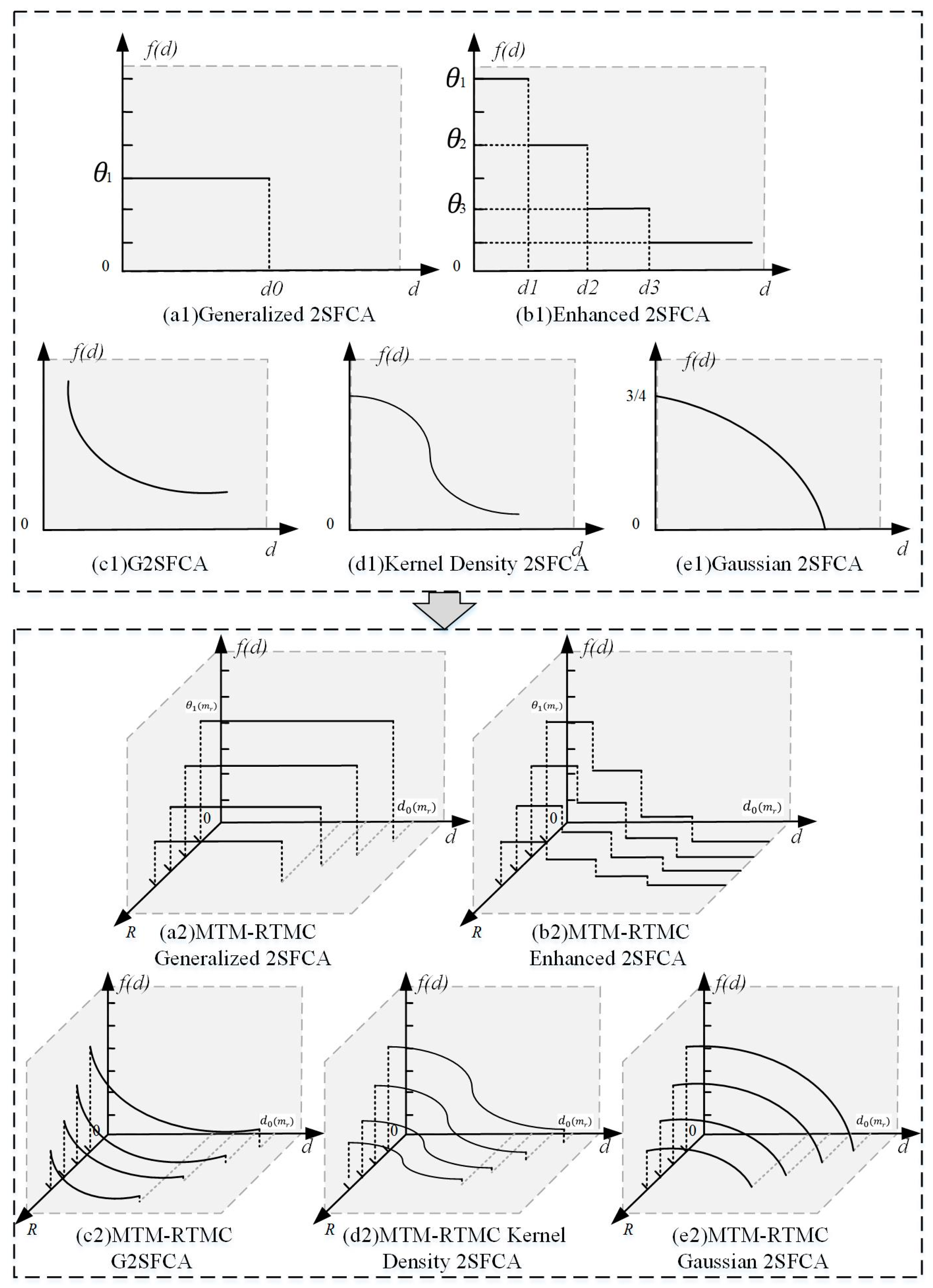
| Model Name | The Distance Decay Function | The Improved Distance Decay Function with MTM |
|---|---|---|
| Generalized 2SFCA | ||
| Enhanced 2SFCA | ||
| G2SFCA | ||
| Kernel Density 2SFCA | ||
| Gaussian 2SFCA |
© 2020 by the authors. Licensee MDPI, Basel, Switzerland. This article is an open access article distributed under the terms and conditions of the Creative Commons Attribution (CC BY) license (http://creativecommons.org/licenses/by/4.0/).
Share and Cite
Zhou, X.; Yu, Z.; Yuan, L.; Wang, L.; Wu, C. Measuring Accessibility of Healthcare Facilities for Populations with Multiple Transportation Modes Considering Residential Transportation Mode Choice. ISPRS Int. J. Geo-Inf. 2020, 9, 394. https://0-doi-org.brum.beds.ac.uk/10.3390/ijgi9060394
Zhou X, Yu Z, Yuan L, Wang L, Wu C. Measuring Accessibility of Healthcare Facilities for Populations with Multiple Transportation Modes Considering Residential Transportation Mode Choice. ISPRS International Journal of Geo-Information. 2020; 9(6):394. https://0-doi-org.brum.beds.ac.uk/10.3390/ijgi9060394
Chicago/Turabian StyleZhou, Xinxin, Zhaoyuan Yu, Linwang Yuan, Lei Wang, and Changbin Wu. 2020. "Measuring Accessibility of Healthcare Facilities for Populations with Multiple Transportation Modes Considering Residential Transportation Mode Choice" ISPRS International Journal of Geo-Information 9, no. 6: 394. https://0-doi-org.brum.beds.ac.uk/10.3390/ijgi9060394