1. Introduction
According to a report by the United Nations Department of Economic and Social Affairs [
1], the percentage of the global population that is urban is expected to increase from the current 55% to 68% by 2050, with the fastest growth in developing countries. This rapid urbanization has resulted in urban overcrowding, reduced green space, and changes in surface pavement, which has exacerbated the negative effects of the urban heat island (UHI) phenomenon [
2,
3]. Apart from the influence of land use and urbanization, extreme heat waves due to global climate change have caused not only higher temperatures but also a significant decline in urban areas’ ability to naturally cool down at night [
4]. This resulted in considerable burdens on cities in the summer or in tropical regions. Therefore, the stakeholders of cities around the world are committed to proposing strategies to effectively modulate the UHI effect.
The strategies proposed to modulate the UHI effect are quite diverse, with construction of a wind field serving as one of the most efficient methods. There is a close relationship between the urban wind field and the UHI effect, and good ventilation can effectively prevent thermal energy accumulation in an urban area [
5]. It can also improve the comfort level of urban street spaces [
6], therefore mitigating the UHI effect. Urban morphology plays an important role in effectively improving the urban wind field. Indicators for urban morphology including urban building density (BD), building height, and building shape [
7]. They are now widely used in relevant urban development regulations under urban plans and laws.
Existing studies on urban morphology and urban wind field construction are conducted at different spatial scales with different research objectives. For small buildings, studies are mainly focused on the interaction of the wind field with the morphology and scale of individual buildings or the layout pattern of neighborhood buildings. However, the scenarios constructed at such scales are mostly focused on the geographical range delineated by buildings themselves and fail to truly reflect the actual, complicated urban morphology. At large regional scales, studies are mainly focused on exploring how to construct a proper wind corridor for the whole city or region, rather than on the morphological setting of individual buildings. On the other hand, when exploring the value changes and their combination for urban morphological indicators during wind field simulation, existing studies lack a systematic scheme for scenario construction. This would make it difficult to attain deeper insights into the impacts of parameter variation on the construction of a wind field.
To fill the knowledge gap, this study selected a part of the overall development zone of the Mass Rapid Transit (MRT) Green Line G12~G13 of the aerotropolisas in Taoyuan City, Taiwan as the study region to simulate urban morphology with an ideal wind field. Scenario construction and data analysis were conducted at the larger scale of several blocks rather than at a building-level scale. In addition, various combinations of urban morphological indicators were used to construct different scenarios. In this study, the CFD method was adopted as an analysis tool. By analyzing the wind field in different simulation scenarios, this study aimed to propose the urban morphological model that would be beneficial to the construction of an ideal wind field and may serve as a reference tool for relevant plan decision-making.
2. Literature Review
2.1. UHI Effect
Continuous urbanization has led to larger urban areas and a higher concentration of urban development, a process accompanied by the disappearance of green spaces and changes in land surface. The influence of land cover types on UHI is significant, as change in land surface temperature would alter the distribution of atmospheric temperature [
3]. The environment of urban could be influenced high solar-radiation absorption rate, release ability and high heat capacity, causing higher accumulation of heat in urban centers than the rural areas [
3]. This phenomenon is referred to as the urban heat island (UHI) effect [
2,
3].
The UHI effect has a significant impact on human life in cities, but the impact of the UHI effect on cities in different climate regions is different. In high latitude regions, the UHI effect does not always produce a negative impact. In winter, it can be considered a positive effect that can reduce energy consumption from heating. However, in tropical regions, the UHI effect directly leads to the risk of heat-related diseases, decreased quality of life, and energy waste, with energy waste mainly attributed to a decrease in operational efficiency of air-conditioning systems [
8,
9]. Given that the UHI effect is an important component of the urban climate and has a direct relationship with the actual morphology of the city, the scientific community has now realized that the negative impact of the UHI effect should be mitigated by urban planning. Mirzaei [
10] conducted an integrated inference and analysis of reported research results on the UHI effect and classified the current main research fields into six categories, namely, changes in urban ventilation and surface physical environment, health and comfort level, spatiotemporal differences in the UHI effect, development of simulation technology, future temperature projection, and building energy conservation.
Changes in urban ventilation and surface physical environment are the research field most relevant to this study. This field is focused on exploring the role of the urban physical environment in mitigating the urban thermal environment. The urban physical environment includes urban morphology and land-use types. Wind circulation plays an important role in the mitigation process, as good ventilation can effectively reduce heat accumulation in a city. Therefore, how to construct a good wind field is an important issue to address in this research field.
2.2. Urban Morphology and Wind Fields
Urban morphological indicators are quite diverse. The most commonly used are floor area ratio (FAR) and building coverage ratio (BCR), which serve as regulatory metrics for building density (BD) and building masses in a city, respectively. The government uses relevant indicators to shape ideal urban morphology as planned. Therefore, if the shaping of urban morphology is to be used as a strategy to mitigate the wind field or the UHI effect, relevant urban morphological indicators would play a key role. Of the studies that consider both wind field and urban morphology, Chiu [
11] investigated the impact of street scale (a metric defined as the ratio of building height to street width, namely H/W) on wind fields. The results show that no matter what the street layout is, the smaller the street scale (H/W), the smaller the change in mean wind speed ratio (defined as the ratio of the wind speed at a location to the basic wind speed in that region, namely U/Ur). Li et al. [
12] conducted simulations of urban wind field using CFD model and detailed building geographical information data, and found that the characteristics of buildings are influential on simulated wind directions and speed in urban areas. Wang et al. [
7] investigated urban wind energy and performed CFD simulation to explore the correlation between 10 urban morphological indicators and wind fields for six real urban forms, trying to obtain the strength of correlation between various indicators and wind field construction. Edussuriya et al. [
13] adopted a large number of analysis indicators, using a total of 21 indicators to analyze the relationship between the diffusion of air pollutants and urban morphology in 20 Hong Kong neighborhoods. Doronzo et al. [
14] developed a method to effectively reproduce the time history of the dynamic pressure of the current and velocity at the flow front, and they found that current can be influenced by mass eruption rate and alimentation duration at the conduit exit. Doronzo [
15] found that pyroclastic density currents strongly interacts with building based on CFD simulations. In addition to the above, CFD model can also be used to study wind field a variety of environments. For example, Doronzo et al. [
16] studied the impact of vertical buildings collapse on currents by applying 3D engineering fluid dynamics. However, there is still limited research on a systematic evaluation of effects of planning factors on wind environment.
2.3. Wind Field Construction
The aforementioned studies on urban morphological indicators and wind fields are mostly focused on correlation analysis. Studies on wind fields, on the other hand, are focused on proposing strategies to improve wind fields through the improvement of building morphology and layout. Huang and Pham [
17] explored the efficiency of the adjustment of building arrangement for improving urban wind and thermal conditions at building-level scales in Thanh Hoa City, Vietnam in a hot, humid climate. They converted the original quadrilateral buildings to streamlined ones and found that by promoting the Venturi effect, wind speed could be increased in the streets, and moreover, the number of dead spaces where wind circulation was absent would be reduced. Rajagopalan et al. [
9] analyzed the urban morphology and wind field of Muar City, Malaysia, through scenario simulation of building height arrangement, finding that a step up configuration was the most effective geometry as it can distribute the wind evenly, allowing the wind to reach inside the city and thereby promoting the mitigation of the UHI effect.
Due to the computational power limitation of the numerical simulation, it is impossible to perform a detailed analysis on the various morphological settings of individual buildings across a large-scale region; therefore, studies at a regional scale are mainly focused on analyzing wind corridors in a large geographical range and proposing possible mitigation strategies. Moreover, such studies adopt more diverse methods than small-scale studies. In addition to the CFD simulation of wind fields, these studies also take advantage of the analytical function of geographic information system (GIS) to perform an overlay analysis of wind fields, urban morphology, and land-use types in a large region. Hsieh and Huang [
5] analyzed the wind field in Anping District, Tainan City, Taiwan, using the frontal area index (FAI) and the GIS-based metric least cost path (LCP), proposing a spatial transformation strategy that was beneficial to the construction of wind corridors.
2.4. CFD Method for Wind Fields
Computational fluid dynamics (CFD) has become one of the main tools for analyzing wind fields owing to the improvement of computer power and computational accuracy, as well as the recent popularization of related software applications [
18]. CFD is currently widely applied to engineering fluid analysis, building design, urban wind fields, and air pollution diffusion [
19,
20]. When performing a CFD simulation of an urban wind field, an urban morphology model or a building structure model should be established as the first step, followed by setting boundary conditions and inputting atmospheric parameters, and then by wind field simulation. Compared with actual measurements and wind tunnel experiments, the CFD method is operationally inexpensive, and CFD simulation results can simultaneously reflect the entire wind field in a given space [
19]. In addition, another major advantage of the CFD method is that it can simultaneously perform comparative analysis among different scenarios, which is impossible using actual measurements and wind tunnel experiments. Although the CFD method is subject to some limitations, such as inaccuracy and divergence in turbulence simulations, it generally can provide good simulation results as validated by wind tunnel experiments or related methods [
7]. ENVI-met software [
21] is used in this study to perform CFD simulation. Since 3D modeling requires the repeated adjustment of indicator parameters, ENVI-met provides built-in modules to allow high-efficiency computation. In addition, although this study was focused on urban geometry and wind field, a variety of land-use types existed in the study region, including farm ponds, parks and green spaces, and farmland. All of which could be well distinguished and properly handled by ENVI-met in the simulation so the results would reflect the overall microclimate.
2.5. Summary
Research on the UHI effect has been conducted from numerous aspects. Given that wind is an important factor of the UHI effect, wind field improvement is considered a very efficient method for mitigating the effect within a large range. The relief of buildings in the city and the urban morphology plays a key role in affecting the urban wind field. In recent research on urban morphologies and wind field construction, the CFD simulation of wind fields has become a prevailing method. However, most studies are focused on building-level scales and fail to reflect the effects of comprehensive planning. On the other hand, most of the mitigation strategies or urban morphological analysis in these studies rely on urban morphological design in a qualitative manner and lack the quantitative support for practical application. Therefore, by using urban morphological indicators to quantify the urban physical environment, it would be possible to address issues that cannot be accurately described in a qualitative manner. Based on this strategy, this study will construct different simulation scenarios using quantitative urban morphological indicators to analyze the wind field and the mitigation of the UHI effect.
3. Research Design
3.1. Study Region
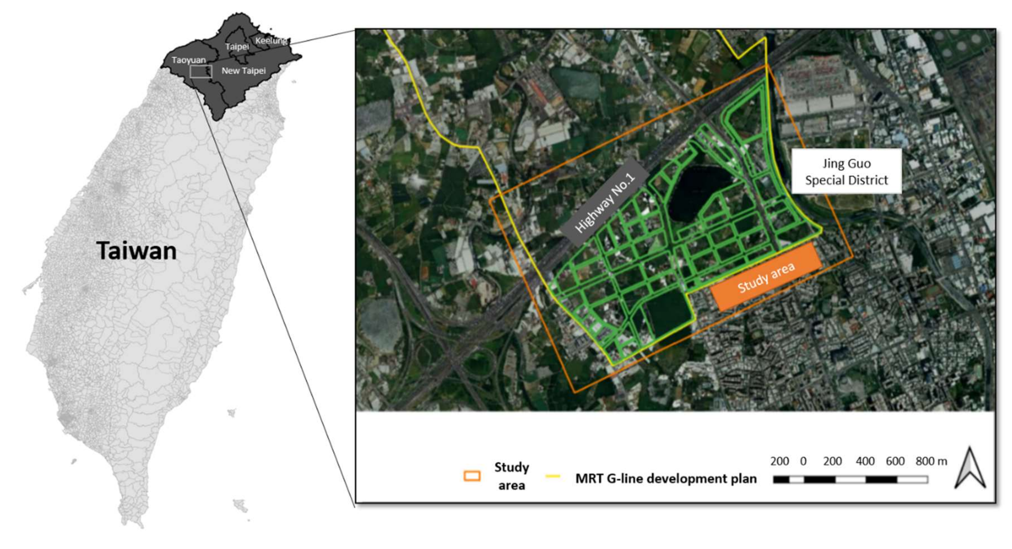
The study region was in Taoyuan City, Taiwan. The site is located south of National Highway No. 1 in the overall development zone of the MRT Green Line G12 ~ G13a, with a total area of approximately 2 km
2 (
Figure 1). In particular, the core study area was about 1.39 km
2 in size, which served as a test zone for establishing and adjusting simulation scenarios in this study. Given that the closer a simulation site is to the boundary, the more likely it is for the simulation to be unstable and have low accuracy [
22], an outer boundary zone is set surrounding the operation zone to ensure the simulation accuracy of the inner operation zone. The overall development zone is developed through zone expropriation. The purpose of the development is to match the development of the aerotropolis project in the North and the planning of transit-oriented development (TOD) around the MRT stations. The project was reviewed and approved by the Urban Planning Commission of the Ministry of the Interior in August 2018, and to date the land has not yet been substantially developed. This allows for considerable flexibility in the adjustment of spatial configuration, which is the main reason for selecting this region as the research region.
Land-use zoning in the operation zone is based on the land-use zoning regulations in the “Detailed Plan for the Nankan New Town Project (to coordinate the development plan for land around the stations of aerotropolis MRT Green Line G12, G13, and G13a of the MRT system in the Taoyuan Metropolitan Area and land around the North Airport)” developed by Taoyuan County in 2013. The detailed plan will be adopted as a baseline plan (plan 0) for the simulation scenario.
3.2. Research Method
3.2.1. Selection of Urban Morphological Indicators
When selecting urban morphological indicators, considerations must be made as to whether the indicators are related to the construction of the wind field. Other considerations include whether they are easy to use and operationally feasible, whether they are applicable at a proper scale, and whether they may be used to provide suggestions for the spatial planning of the study region. The indicators selected in this study were described separately as follows.
• Floor area ratio and building coverage ratio
Floor area ratio (FAR) and building coverage ratio (BCR) play a very important role in current urban planning laws and regulations, which directly control the development density, height, and open space size of urban buildings. These provide strong guidance for the evolution of urban morphology. Accordingly, this study used FAR and BCR as the tuning parameters for the simulation scenario construction, aiming to provide suggestions on the application of these two important indicators to the construction of wind fields and the mitigation of the UHI effect. In the meantime, this study also used these parameters to reveal the overall urban space changes along the horizontal and vertical dimensions or the changes in building masses through these two indicators as metrics of urban planning, thereby providing an important reference for urban morphological analysis. The two indicators are elaborated separately as follows.
FAR
FAR refers to the ratio of the total floor area of buildings in a district to the site area upon which the buildings are built, which can be calculated using Equation (1).
BCR
BCR refers to the ratio of the total area of the building footprints to the site area upon which the buildings are built, which can be calculated using Equation (2).
Ai represents the footprint area of the ith building, Ni the number of floors in the ith building, and S the site area in a district. The prerequisite for using this formula is that each floor of a given building has the same area.
• Building density (BD)
The concept of building density (BD) originates from landscape metrics in landscape ecology, which are constructed using a number of spatial elements, including patch, corridor, and matrix, in order to evaluate spatial and temporal changes of land cover in landscapes [
23]. Landscape metrics can be classified as metrics at four different analysis levels, namely cell-level metrics, patch-level metrics, class-level metrics, and landscape-level metrics, in order of increasing level. In particular, class-level metrics are intended for the overall analysis of certain types of patches with a focus on the mean properties of the patches, such as mean area and mean density [
24]. Such patches constitute a spatial framework similar to that used for analyzing the morphology and spatial layout of buildings in this study. However, the whole system of landscape metrics is quite complicated and not completely suited to this study. Due to technical constraints, this study includes only one class-level metric in the tuning parameters for constructing simulation scenarios.
Patch density (PD) refers to the number of the same type of patches per unit space, which measures the degree of fragmentation of a landscape pattern [
25]. In this study, patches refer to buildings, and accordingly, PD will be used to evaluate whether the building space layout is centralized or scattered. Given that this study focuses on buildings, PD will be referred to as BD hereafter. In the following calculation formula [
25], BN represents the number of buildings and A represents the unit area.
• Mean building height and its coefficient of variation
The building height of a city directly affects the appearance of the skyline, with different cities having different building-height patterns. Moreover, building height is of pivotal importance to the research issue of this study. Wang et al. [
7] conducted a correlation analysis between ten urban morphological indicators and the simulation results of wind fields at six test cities of dramatically different urban morphologies. The results show that building height-related urban morphological indicators showed relatively significant correlations with simulated wind field when compared with other types of urban morphological indicators, with the former indicators including mean building height and standard deviation of building height. This indicates that building height plays a significant role in the construction of an urban environment, and the two building height-related indicators suffice in presenting the vertical pattern of a city. The two indicators are addressed according to Wang et al. [
7], as follows.
In this study, five indicators are selected, which are classified as either horizontal parameters (BCR, BD) or vertical parameters (FAR, , coefficient of variation of mean building height) to facilitate parameter tuning in subsequent scenario simulation.
3.2.2. Establishment of Operation Scheme for Scenario Simulation
After selecting the tuning parameters for scenario simulation, the next step is to construct simulation scenarios according to an operation scheme and perform numerical simulation and analysis.
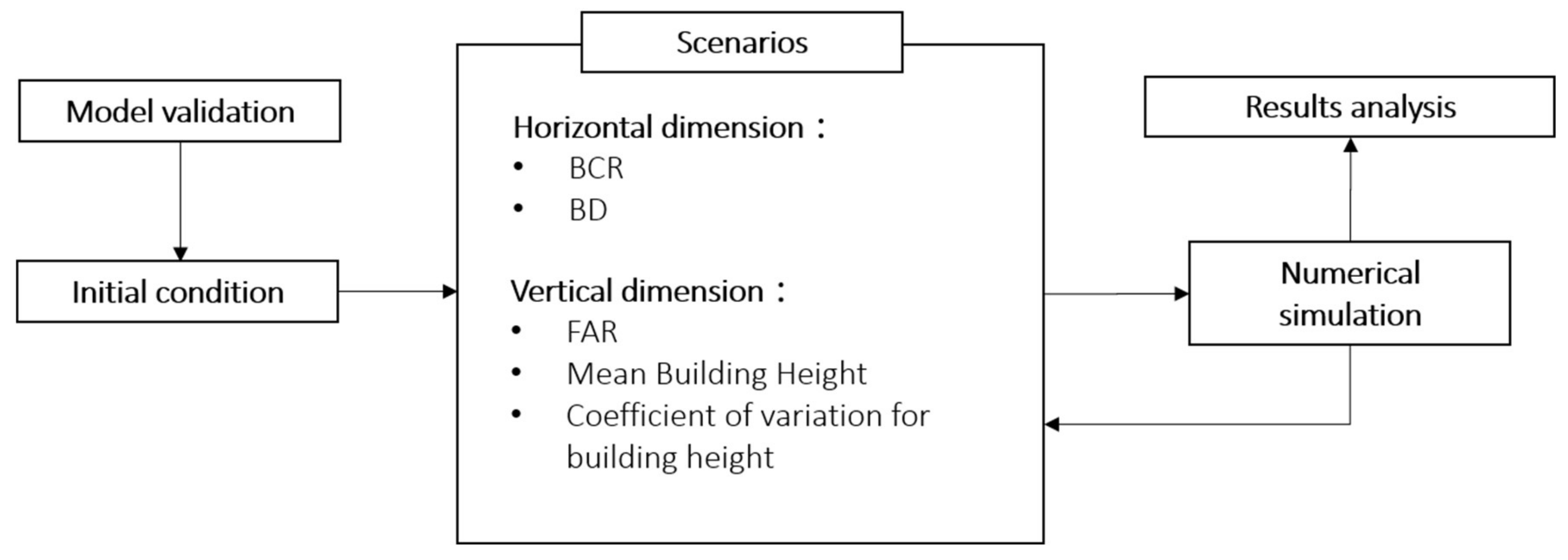
Figure 2 presents the operation scheme for constructing simulation scenarios. First, an initial plan-zero scenario was constructed according to the land-use zoning regulations (BCR and FAR) defined by the Taoyuan County government’s detailed plan for the zone in 2013. Other scenarios were constructed by tuning the parameters as appropriate.
The entire operation process forms a loop in which relevant parameters are modified according to the simulation results for a given scenario. Through iterative parameter tuning, this study aims to construct the urban morphology of a good wind field able to alleviate the UHI effect. In the meantime, to explore the possible significance of metrics relevant to the construction of a wind field.
3.2.3. Numerical Simulation (ENVI-Met)
ENVI-met is a software developed for the 3D CFD simulation of an urban microclimate and can handle the interaction of plants, water, and air. Its basic spatial resolution is 0.5–10 m with a time resolution of 1–5 s, and the simulation time can range from 24 h to 48 h [
26,
27]. ENVI-met version 4.4.1 was used in this study. The simulation space of ENVI-met was made up of three independent submodel grids (
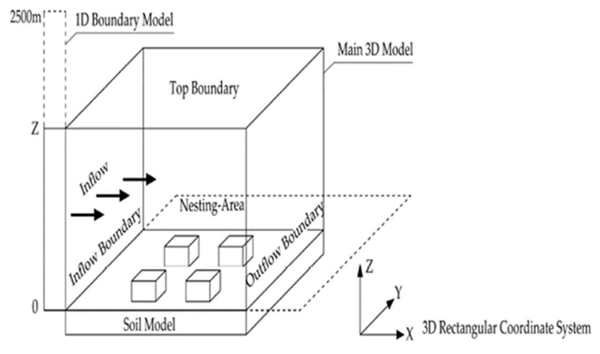
Figure 3) corresponding to a one-dimensional boundary submodel, a three-dimensional submodel of the main body, and a soil submodel. The one-dimensional boundary submodel was to ensure simulation accuracy at high-altitude boundaries. However, due to an overly large number of grid cells, the computational efficiency was low, so the one-dimensional submodel extended from the top boundary of the 3D main-body model to the height of 2500 m. The main-body 3D submodel was mainly used to simulate the spatial configuration of various elements, which included buildings, plants, and different surface pavements, and the main body is also the space for atmospheric simulation. In this space, all elements are presented in the form of grid cells, with the size of the grid cell ultimately determining the spatial resolution of the simulation results. The soil submodel is used to calculate the conversion of geothermal energy and the evapotranspiration from soils and plants. For detailed calculation formulas, please refer to the user manual of ENVI-met [
28].
4. Model Validation and Simulation Results
4.1. D Grid-Cell Setting
As previously mentioned, the characteristics of the ENVI-met software have resolution ranges from 0.5 to 10 m. In most studies performed at building and neighborhood scales, a highest resolution of 0.5 to 1 m is usually used. In this study, the simulation range is approximately a 2000 × 1000 m2 square, which is many times larger than the single streets in other studies at building and neighborhood scales. To ensure high-resolution simulation results while comprehensively considering the large-scale range, the number of grid cells, and the computer’s computing power, this study set the number of horizontal grid cells to X = 249 and Y = 164 with a horizontal resolution of 8 m while gradually increasing the size of vertical grid cells from the minimum 3 m in the bottom layer to greater values at higher layers to reduce the total number of grid cells.
4.2. ENVI-Met Model Validation
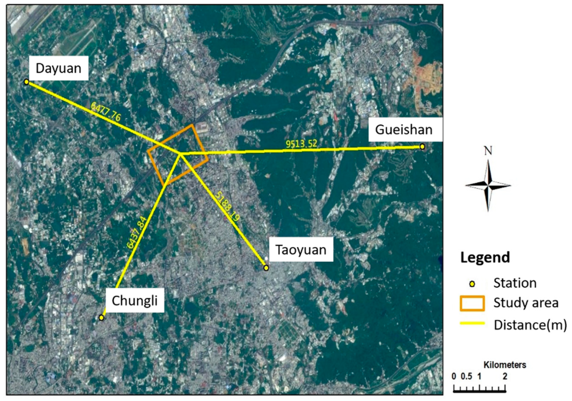
Before scenario simulation, the first step is to ensure the accuracy and reliability of the simulation tool, so the validation of simulation software is an important and necessary process. In this study, model validation is performed using wind speed, temperature and relative humidity data. The validation data were obtained using Kriging interpolation. The reason for doing so was that if observation data were obtained through on-site measurements, the time scale of the validation data would not be long enough and thus the validation data would be of low reference value [
29]. Before interpolation, the number and location of the stations must be determined. In this study, four stations within a 10-km radius of the study region were selected, namely Taoyuan, Chungli, Dayuan, and Gueishan (
Figure 4). The time series of the validation data are complete 24-h meteorological data from 8 July to 9 July, 2018, and the selection of these two days was based on the consideration that summer days with cloudy weather, rainfall, or typhoons should be excluded, as these types of weather are uncontrollable variables for the simulation software. The meteorological data for constructing the model were obtained from the Taoyuan station, which is the closest of all the four stations to the study region. The model validation data were generated by performing Kriging interpolation on monitoring data from the four stations. Given the relatively simple status of the study region and the limited differences in simulation results, systematic sampling was performed at intervals of 50 grid cells in horizontal and vertical directions (
Figure 5), and sampled cells that are outside the study region are excluded from further analysis.
Quantitative analysis was performed using root-mean-square error (RMSE), which is quite suitable for examining the degree of congruence between simulated and monitored data [
30,
31], as RMSE can present the overall mean error of simulated data with respect to observed data.
where
is the observed value at monitoring point
i, and
is the modeled value at point
i, and n is the number of sampling points.
However, such a mean error parameter cannot be used as an evaluation criterion of simulation accuracy alone, as RMSE calculated that using a given set of monitored data is only meaningful for this set of data and cannot be compared with RMSE derived from another set of data [
28]. In addition, the range of RMSE varies when applying to different datasets, making it difficult to set threshold criteria. To solve this problem, Willmott [
28] developed the Index of Agreement (
d), which takes a value between 0 and 1.
where
is modeled value,
is observed value, and
is the mean of observed value.
The more the value of
d approaches 1, the more similar the simulation results are to the monitored data; conversely, the more the value of
d approaches 0, the worse the simulation’s performance [
32].
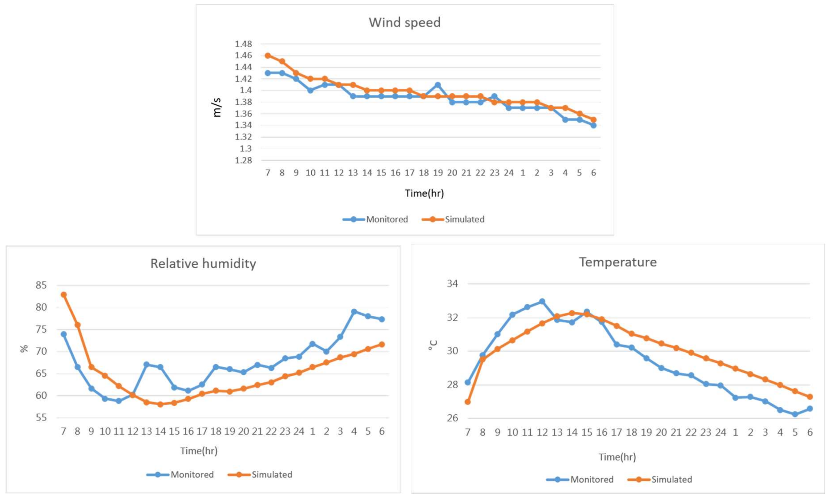
Table 1 presents the RMSE and d-values of model validation. When using
d as the evaluation criterion, studies [
30,
31] accept that
d-values greater than 0.8 are of reference significance for the evaluation of model validation results. According to this viewpoint, the model performed quite well for wind speed and temperature simulation in this study. For relative humidity, the
d-value was lower than 0.8, but it was still of reference significance. Time series of the validation data are shown in
Figure 6. On the whole, the simulation results were of reference significance for the trends of wind speed, temperature and relative humidity.
4.3. Simulation Scenario Setting
The construction of the initial scenario was based on the land-use zoning regulations provided in the detailed development plan for this region. Given that the current developers would often strive for additional FAR or FAR transfer on top of the baseline volume to maximize development benefits, the simulation scenarios that are constructed solely based on the baseline volume fail to truly reflect the actual situation. The third provision of Article 42 of the "Taoyuan City Implementation Rules of the Urban Planning Act" states that after transferring and adding building volumes to a building site, the total FAR should not exceed twice the original base FAR. Therefore, to mimic the true development situation as much as possible, the simulation scenario was set to have an initial FAR twice the upper limit of the base FAR, and the initial FAR may later be adjusted—mainly downsized. However, exceptions applied to some land-use types, such as school land, in the study area. Since such types of land fall into the category of public facilities, and accordingly the developers would be less likely to pursue additional building volumes, the base volume was adopted for such land types in this study. In contrast, the initial simulation scenario was set to have the legal upper limit of BCR. As there were no zoning regulations on the other two indicators, they were first set to certain values and then adjusted as appropriate. Considering that the coefficient of variation for building height measures the degree of height difference among buildings, a scenario without building height differences was first simulated, followed by simulation of a different scenario where building height differences were adjusted to be significant. The difference in UHI effect between the two scenarios can thus be revealed. BD reflects the degree of fragmentation of the spatial distribution of buildings. The setting of FAR and BCR in the initial scenario was intended to lead to the highest BD and the least amount of open space. To make the buildings the most crowded and minimize the ventilation space between buildings at the maximum permitted BCR, 2.5 buildings per hectare represented the largest BD given the current three-dimensional modeling ability of this study. In the case of a non-integer number of buildings in the calculations, the number would be rounded to the nearest integer. According to the above principles, parameters were set for simulation scenarios as outlined in
Table 2, with examples of building model settings illustrated in
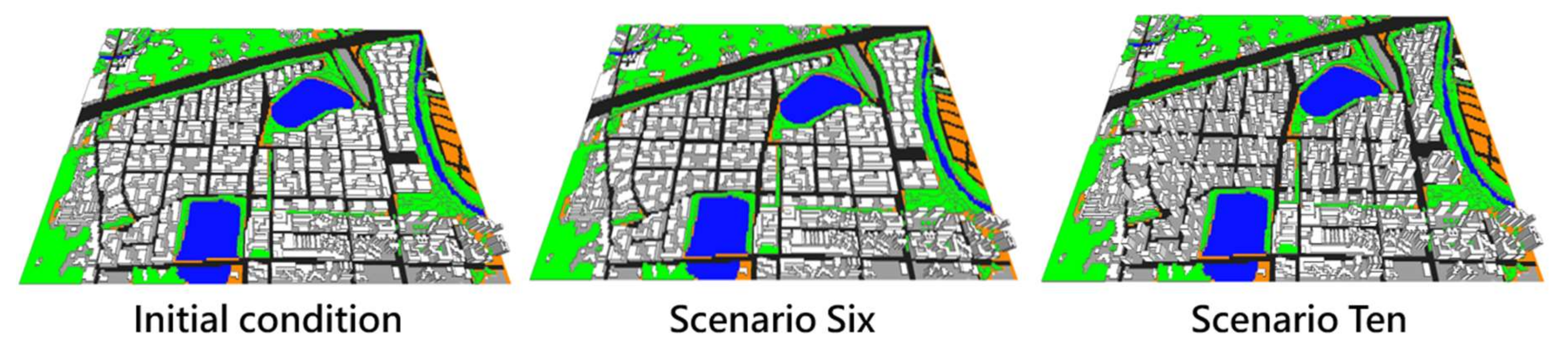
Figure 7. It could be seen in
Figure 7 that the in initial condition scenario, building coverage ratio is set to be the uppper limit of current planning regulation, resulting in much denser building footprints than the other two. Scenario 6 represents the condition where floor area ratio is set to be two times as the initial condition, thus resulting in higher buildings in the region. Scenario 10 repsents the case with lower building coverate ratio, 1.5 times FAR and higher coofficient of variation for building height, forming a much diversifed urban landscape than initial condition and scenario 6.
Before the modeling process, proper setting of the input boundary conditions are important for the purpose of making the simulated environment more consistent with the actual one. Data derived from the nearby monitoring stations were used to set the boundary conditions as shown in
Table 3.
4.4. Results of Scenario Simulation
In each of the 12 scenarios, 24-h time series (8 am to the next 8 am) of hourly wind speed were simulated using ENVI-met. As for data analysis, since this study was focused on scenario simulation for an undeveloped region, there were no specific points of interest to be comparatively analyzed. On the contrary, to present the overall situation of the entire region, all grid data within a certain range would be averaged. This range was selected to be 1.5 m in the vertical direction because this is the vertical range of the atmospheric environment that residents are exposed to in urban open spaces. In the horizontal direction, to avoid interference from less accurate grid cells near the boundary and given that the analysis was limited to within the operation zone, this study ignored the data of outer grid cells. Results of different scenarios are compared in the following sections.
4.4.1. Wind Field Analysis
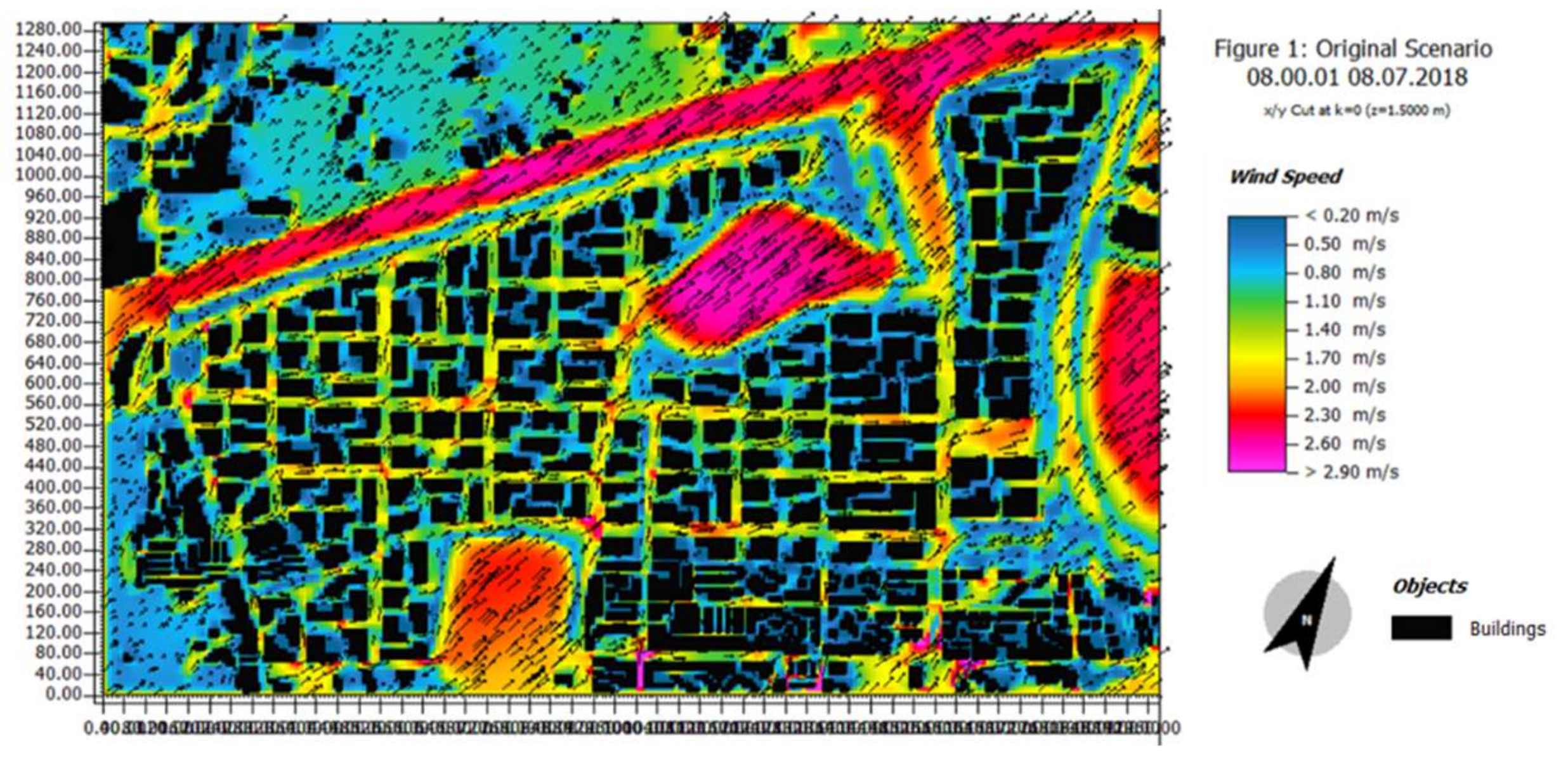
Figure 8 presents the simulated wind field at 8 am in the initial scenario. The black areas represent the distribution of buildings, and the color bar represents the strength of the wind speed, with the black arrow showing the wind direction. As shown in
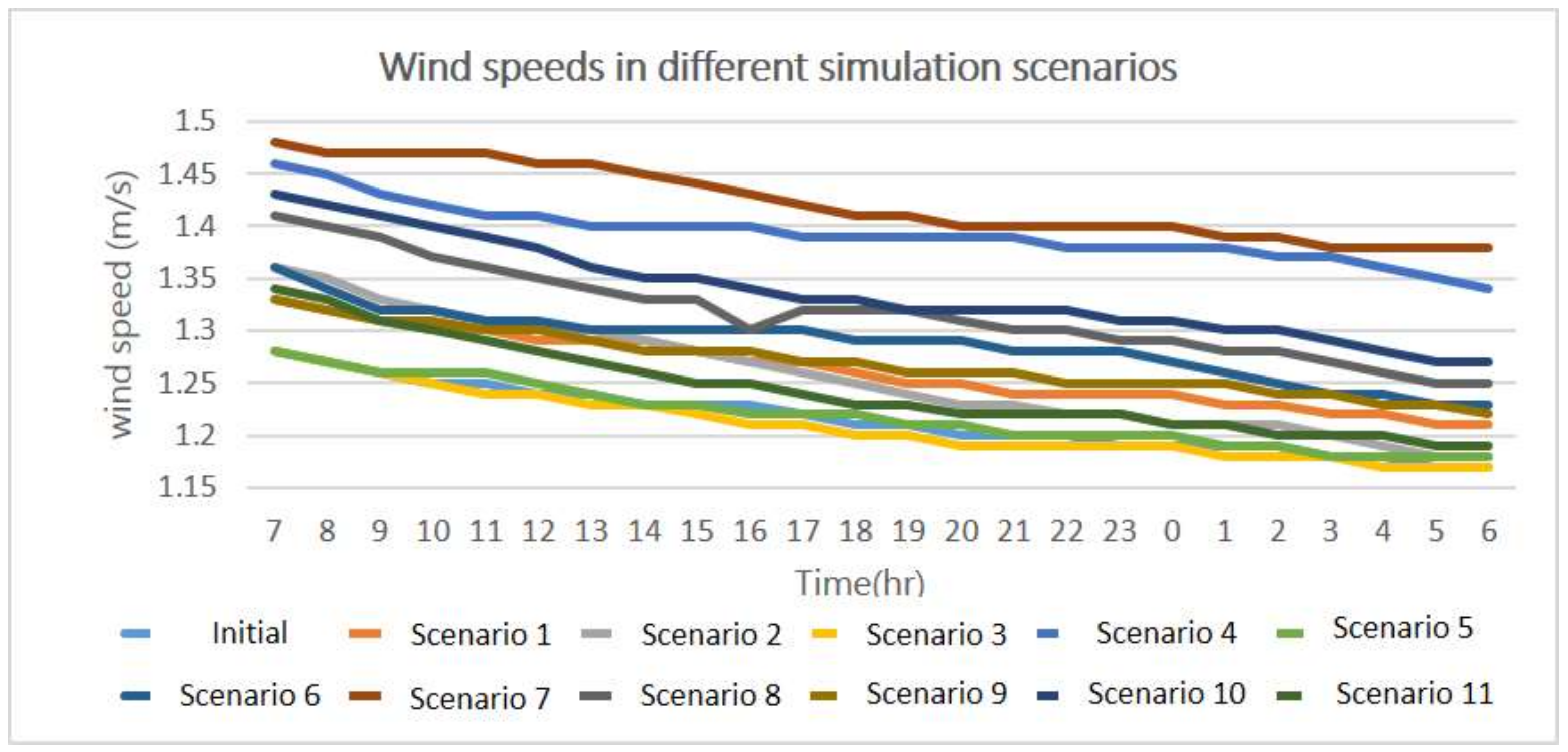
Figure 8, the highest wind speed was located at two farm ponds, a patch of bare land on the west border, and a north highway. The possible reason why wind speed at highway is relatively high is that the elevated highway created a wind corridor underneath without the blocking effect of buildings. The areas with slow wind speeds were mainly distributed outside the operation zone and the current land-use type is agricultural land. This indicates that short crops have a significant effect on the simulation of a wind field within a vertical 1.5-m-high range. In the operation range, the main road between two adjacent blocks is subject to a significant street canyon effect under significantly high wind speeds. Within a block, the space adjacent to buildings has low wind speeds. According to the aforementioned method for plane data acquisition, the mean hourly wind speed in each scenario during a 24-h period was obtained and illustrated in
Figure 9, which shows that the wind speed in each scenario slowly decreased with time and approached a stable level. On the whole, the changes in wind speed over a 24-h period were not obvious, but there were significant differences in mean wind speed among various simulation scenarios. The largest differences were found to be between Scenario 3 and Scenario 7, indicating varying the all of the 4 parameters at the same time did result in the greatest variation. The difference between Scenario 3 and Scenario 4 appears to be relatively small, suggesting that the influence of BD might not be as significant as the other parameters. In addition, the reason why there is no periodic change in wind speed overtime might be because that according to historical data, regional wind speed and direction in a day were relatively stable. The 24-h-averaged mean wind speed was used to further compare simulation results among various scenarios with different urban morphological indicators.
4.4.2. Simulation Results under Different FAR
For simulated wind speeds under a FAR 2 versus 1.5 times the base FAR, there were six pairs of simulation results to compare according to the aforementioned scenario settings (
Table 4). Overall, when the coefficient of variation for building height was 0, the decrease in mean building height due to a 25% decrease in FAR led to an increase in overall mean wind speed by about 5%.
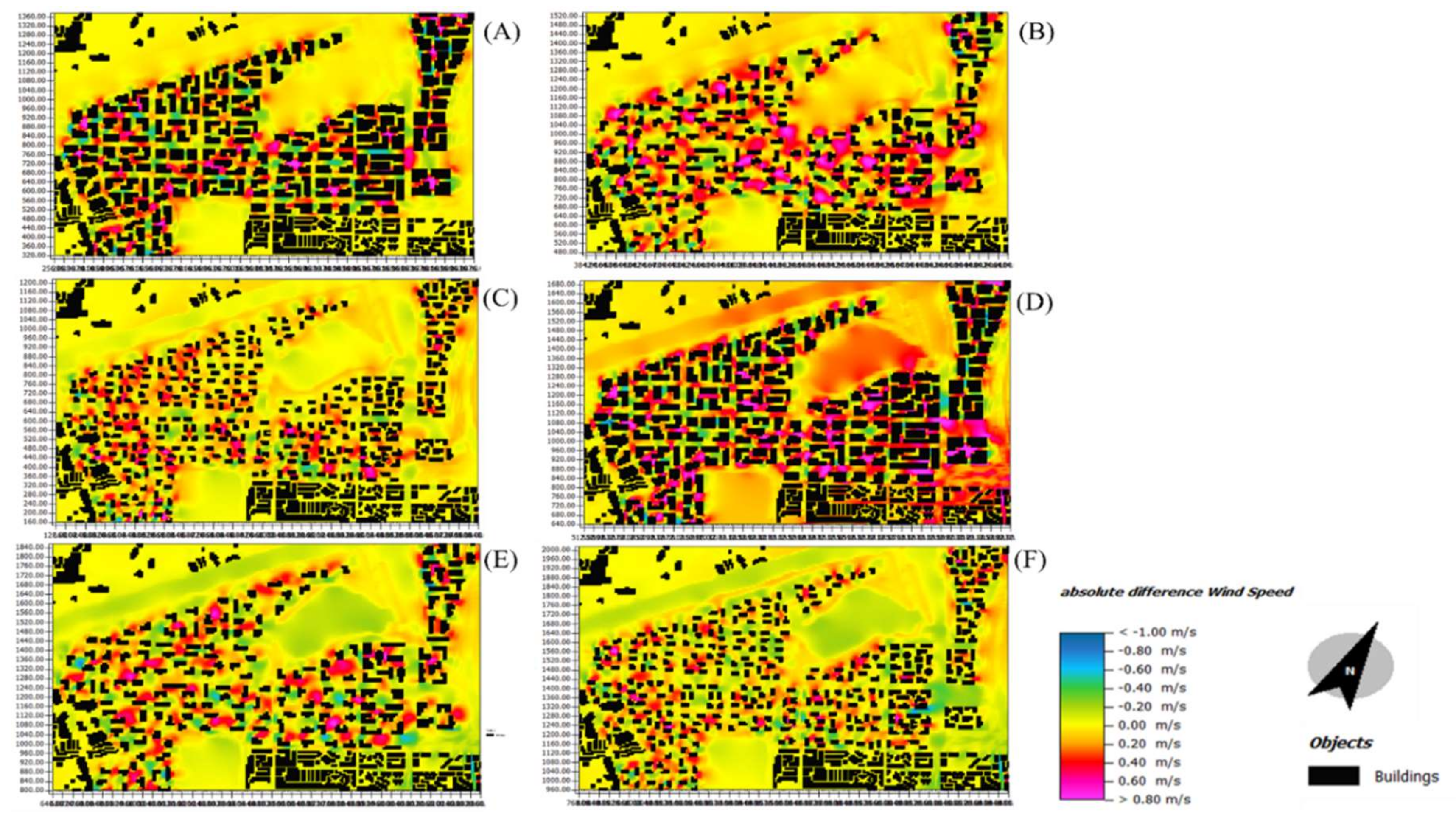
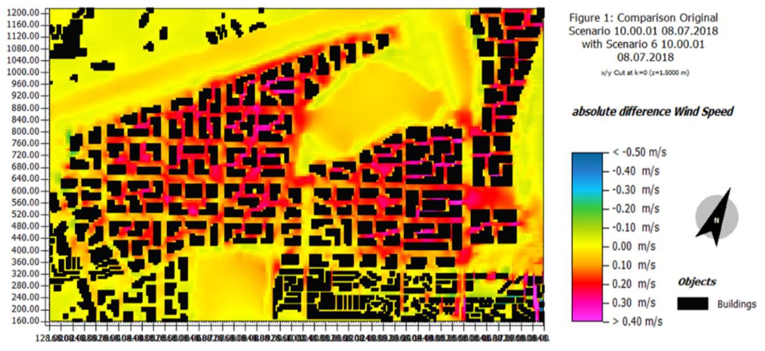
Figure 10 presents the spatial distribution of the wind speed differences between the initial scenario and Scenario 6. It can be seen that whether on streets or between adjacent buildings, there were significant differences in wind speed, indicative of a significant effect from FAR on the spatial distribution of wind speed in each district. This further confirms that it is feasible to adjust an urban wind field by adjusting FAR.
4.4.3. Simulation Results under Different BCR
Table 5 presents simulated wind speed in four pairs of scenarios with different BCR values. Comparison of the initial scenario (high BCR) versus Scenario 2 (low BCR), as well as Scenario 6 (high BCR) versus Scenario 8 (low BCR) indicated that simulated wind speed was higher by 2%–3% in the case of low BCR than in the case of high BCR. There was a large wind speed difference between Scenario 1 (high BCR) and Scenario 4 (low BCR), with the simulated wind speed being higher by nearly 10% in the case of low BCR than in the case of high BCR. In the pair of Scenarios 1 and 4, the coefficient of variation for building height was 60%, much higher than the comparative 0% in the above two pairs of scenarios.
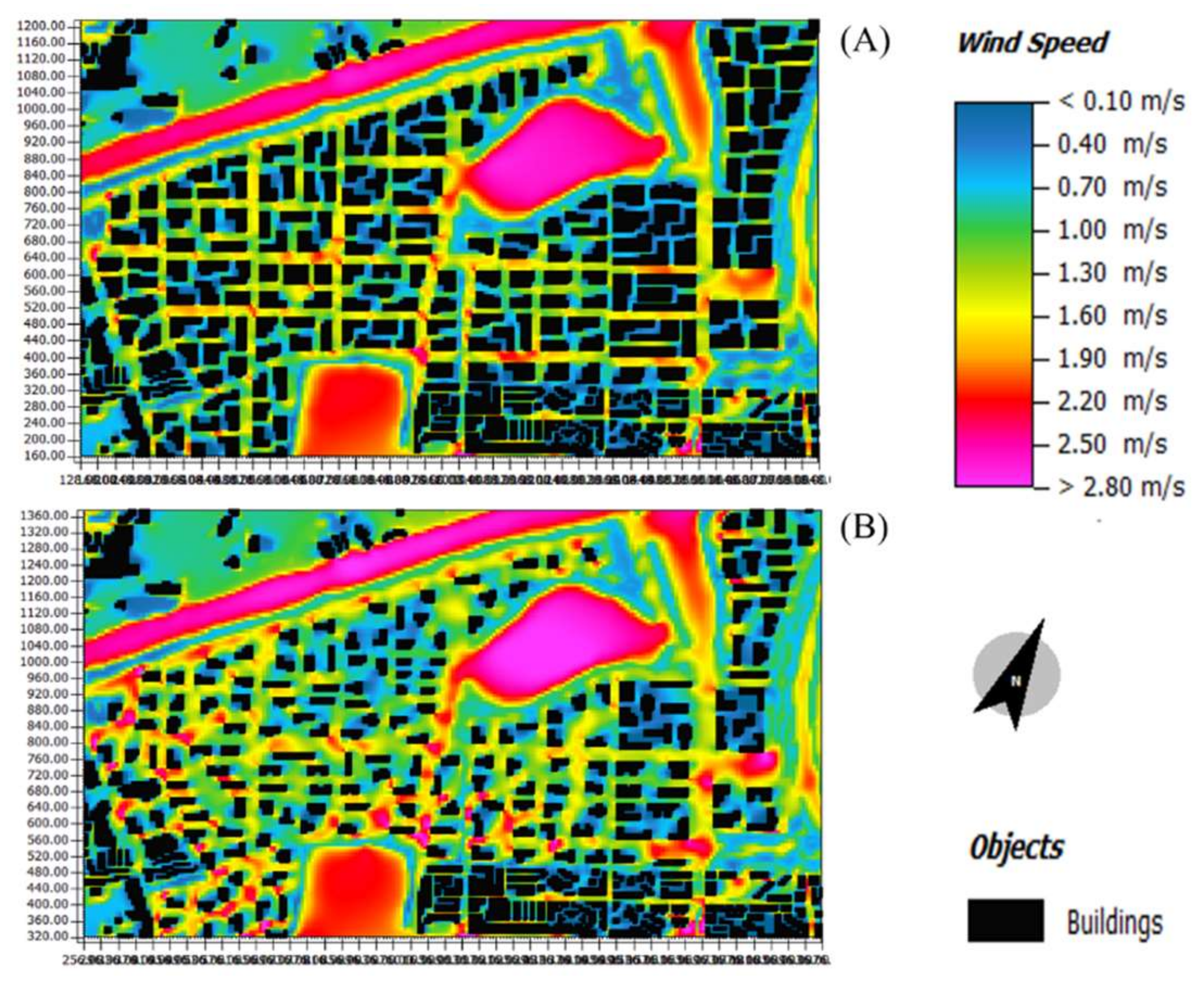
Figure 11 presents the distribution of simulated wind speed in the initial scenario versus Scenario 2, indicating that the overall impact of BCR on wind speeds was non-linear. The overall wind speed in some areas (such as some blocks in the southeast) increased due to the decrease of BCR. However, in the northwest of the base, some areas did not show significant changes in wind speed when BCR decreased. This observation indicates the importance of using CFD models to perform detailed simulation, which can provide deeper insights into the differences between areas.
4.4.4. Simulation Results under Different BD
BD reflects the concentration and dispersion of building masses. As shown by the data in
Table 6, simulated wind speeds were higher in the case of low BD than in the case of high BD. In terms of the magnitude of change, wind speed changes greater than 4% were observed between Scenario 2 and Scenario 3. Similar results were found between Scenario 8 and Scenario 9. While the change was as high as 13% between Scenario 4 and Scenario 5, and was lower (but still relatively high) at 6% between Scenario 10 and Scenario 11. The changes between the latter two pairs of scenarios were dramatically different from the changes of about 4% between the former two pairs of scenarios, which was attributed to the same reason as for the aforementioned wind speed changes under different FAR. That is, Scenarios 2 and 3 as well as Scenarios 8 and 9 had a high coefficient of variation of 60% for building height compared with other scenarios. This showed different and even extreme changes in wind speed compared with other scenarios.
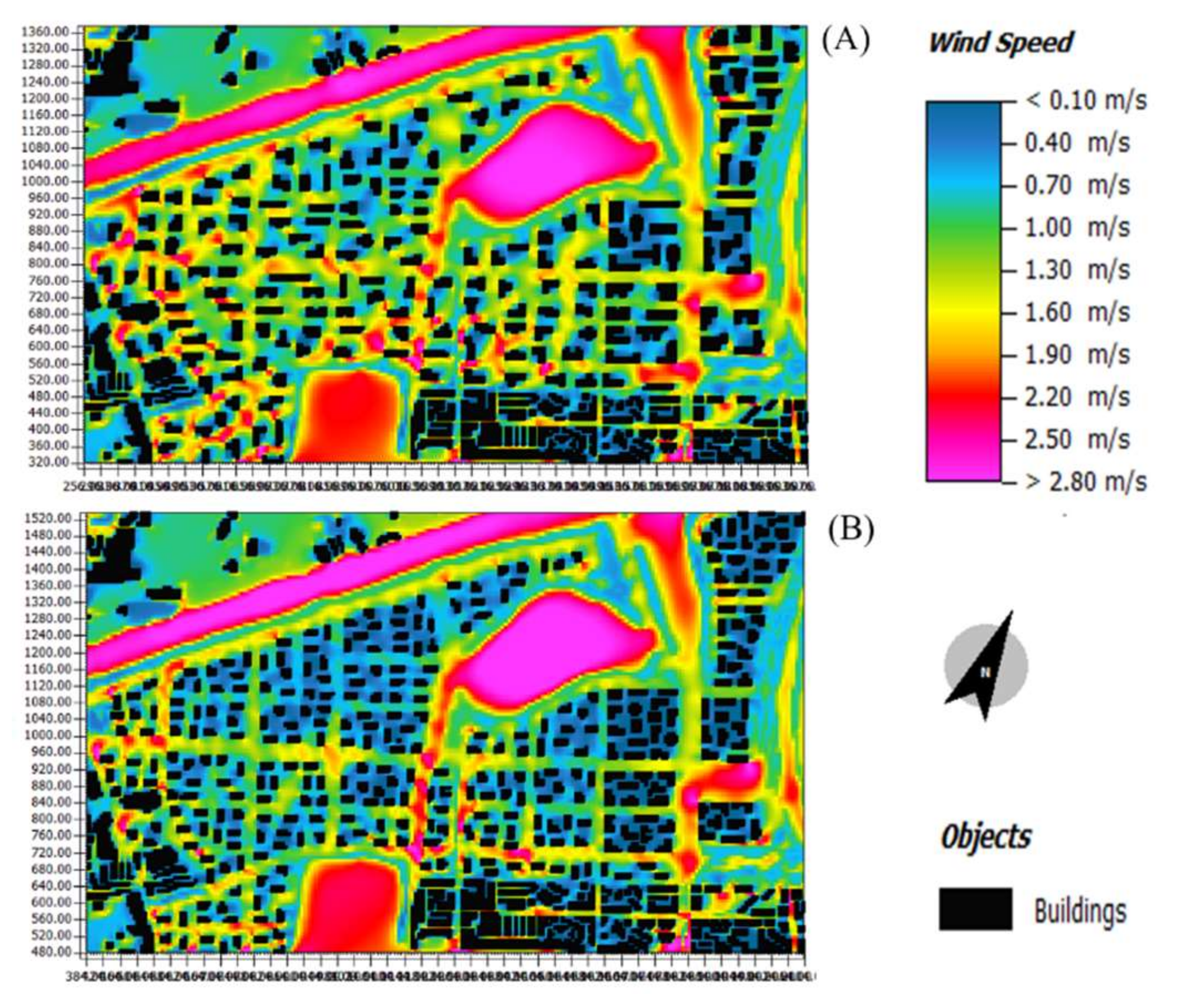
Figure 12 presents a comparison of simulated wind fields between Scenario 2 and Scenario 3. It clearly shows that BD had a significant impact on the spatial distribution of wind speed, especially in low-BD scenarios where the wind corridors formed by the spaces between buildings. This led to a certain degree of improvement in inter- and intra-block ventilation, confirming that BD is indeed an important factor to consider when planning the overall wind field of this development zone in the future.
4.4.5. Coefficient of Variation for Building Height
As shown in
Table 7, wind speeds in scenarios with a 60% coefficient of variation for building height showed dramatic changes compared with scenarios with a 0% coefficient of variation, with the changes being both positive and negative and randomly distributed in the space (
Figure 13). The comparison between the scenario with a building average height coefficient of variation of 0 and the scenario with a 60% building average height coefficient of variation is shown in
Table 6. It shows that the latter produces a fairly significant change in wind speed, and this change is to strengthen and weaken the staggered random distribution in space (
Figure 13). This spatial distribution pattern was attributed to the way of setting the simulation scenarios, namely maximizing the overall difference in building height while evenly distributing different building heights across the region. Although the scenario-averaged mean wind speed of the scenarios with a 60% coefficient of variation for building height was higher than that of scenarios with a 0% coefficient of variation, the mean wind speed per se showed large differences among the former scenarios. In addition, there was not a simple relationship between the differences and the scenario parameters. In particular, 50% of the buildings in Scenario 7 with a 60% coefficient of variation for building height were only two or three stories high, which allowed the wind to more efficiently flow into the ground floor environment compared to other scenarios, thus significantly increasing the wind speeds. This observation indicated that building height had no obvious and consistent effects on wind speeds, which may be attributed to the fact that wind speed sampling was mainly conducted near the ground surface in this study.
5. Discussions
As shown above, the scenario parameters of FAR, BCR, BD, and coefficient of variation for building height had different degrees of impact on wind speeds. First of all, as far as the impact of FAR on wind speeds is concerned, the decrease in mean building height due to a 25% decrease in FAR led to approximately a 5% increase in the 24-h-averaged mean wind speed of the whole region when the coefficient of variation for building height was 0%. Moreover, the increase in 24-h-averaged wind speed was evenly distributed in the region. As far as the impact of BCR on wind speeds is concerned, wind speeds in scenarios with a BCR 0.5 times the legal upper limit increased by about 2%-3% and by 10% compared with other scenarios with the legal upper limit of BCR when the coefficient of variation for building height was 0% and 60%, respectively. It shows that reducing BCR can effectively increase urban wind speeds and, in turn, may lead to urban cooling and improved comfort. In addition, as far as the impact of BD on wind speeds is concerned, this study revealed that the mean wind speed decreased by about 4% when BD increased from 2.5 buildings per hectare to 5 buildings per hectare when the coefficient of variation for building height was 0%. This suggests that a higher degree of block fragmentation leads to a greater obstacle to wind circulation even in an open space of the same size. Finally, when it comes to the impact of building height on wind speeds, wind speeds underwent dramatic changes from scenarios with a 0% coefficient of variation for building height to scenarios with a 60% coefficient of variation for building height, and the changes were both positive and negative, showing a random spatial distribution. This spatial distribution pattern was attributed to the way the simulation scenarios were set, namely maximizing the overall difference in building height while evenly distributing different building heights across the region. Although the scenario-averaged mean wind speed of the scenarios with a 60% coefficient of variation for building height was higher than that of scenarios with a 0% coefficient of variation, the mean wind speed per se showed large differences among the former scenarios. There was not a simple relationship between the differences and the scenario parameters. In particular, half of the buildings in Scenario 7 with a 60% coefficient of variation for building height were only 2 or 3 stories high, which allowed the wind to more efficiently flow into the ground floor environment compared with other scenarios, thus significantly increasing the wind speeds.
In addition, the simulation results revealed that the impact of any of the above factors on wind speeds was non-linear, and the impact varied significantly among different areas of the study region. These observations confirm the importance of using models to simulate the impacts of urban morphology on wind speeds, as such an approach can provide more accurate and detailed information about the impacts of building masses on wind speeds. Simulation of the differences in regional wind speeds among different planning scenarios can provide strong decision-making support for alleviating and adjusting the UHI effect or air pollution under the influence of the urban wind field.
6. Conclusions
In this study, simulation scenarios were constructed for a new development zone by using urban morphological indicators, and the impacts of these indicators on wind field and air temperature were analyzed using CFD simulation. As far as development factors are concerned, FAR and BCR were the two most important indicators in the zoning regulations for planned urban land use. Scenario simulation revealed that low FAR and BCR would promote the construction of a favorable wind field. However, these two indicators are of planning importance. For any new development zone, there is a pre-set goal for development intensity and density, with FAR and BCR serving as the most direct tools for regulating the development. Therefore, there is not much room for adjusting FAR and BCR. The other two indicators, BD and the coefficient of variation for building height, are currently not subject to direct legal regulations, and the simulation results showed that low BD would also promote the construction of a favorable wind field, while a high coefficient of variation for building height would lead to complicated fluctuations of the wind field, with wind speeds increasing in some areas and decreasing in others.
This study analyzed the wind field’s sensitivity to each indicator. However, when applying the analysis results to the construction of the wind field, the interplay of the indicators should be considered in addition to the aforementioned planning requirements for FAR and BCR. For example, a different BD would lead to significant differences in the wind field under the same BCR. Therefore, the construction of the wind field should not be solely based on a single factor. That is, when applying the four indicators to the construction of the wind field, it is necessary to first conform to the FAR and BCR regulations in order to meet the requirements for development intensity, and then adjust the factors to promote the construction of a favorable wind field. As far as BD and the coefficient of variation for building height are concerned, the former may be reduced under different combinations of FAR and BCR to make the open space more concentrated. The latter may be set to different values to change building height and make the changes perturb the wind field in a favorable manner, which would ultimately improve the wind field in areas where urban ventilation is desired, such as important pedestrian walkways. Implementation of the latter two indicators may be included in the criteria for urban design review. As regulated in the detailed development plan for the study region, the construction and development of building sites above a certain size and of public facility land such as parks and green spaces should be reviewed and approved by the urban planning commission.
The four urban morphological indicators were used to construct a total of 12 scenarios for the new development zone, and the sensitivity of the overall wind field to each indicator was analyzed. The results showed that in scenarios where the mean building height was 0 and coefficient of variation for building height is 0, a 25% decrease in FAR would lead to an increase of about 5% in overall mean wind speed. This wind speed increase was spatially uniform across the zone. A 50% decrease in BCR would lead to an increase of 2%-3% in mean wind speed. When BD was reduced from 5 buildings per hectare to 2.5 buildings per hectare, the mean wind speed increased by about 4%. Wind speeds in the scenarios with a 60% coefficient of variation for building height were significantly promoted or weakened compared with scenarios with a 0% coefficient of variation for building height, with the wind speed differences unevenly distributed across the zone.
Although the wind field in a scenario may not have a certain degree of mitigating effect on urban heat islands, an improvement in the wind field can still enhance the perceived thermal comfort of the external environment. Therefore, this study proposes that metrics relevant to the wind field should be included in the land-use zoning regulations or the criteria of the urban design review for a new development zone. Moreover, it is necessary to take into account the wind direction and wind speed when conducting land-use zoning. This is to ensure that the zoning of land-use types capable of adjusting air temperature, such as parks, green spaces, and bodies of water, will be harmonious with the wind field.
On the other hand, this study focuses on mitigating the UHI effect through wind field construction, since the UHI effect is an urban microclimatic phenomenon closely related to water, vegetation, and pavement. Therefore, it is desirable to analyze the joint impact of the above elements and urban morphologies on the UHI effect in follow-up research. In terms of the actual impact of wind speed on UHI, the desirable threshold of wind speed for mitigation vary from places to places due to various climatic and geographical conditions. For example, Hathway and Sharples [
33] found that temperature increased when wind speed increased in the study area in UK. However, Brandsma and Wolters [
34] found that low wind speed resulted in higher UHI temperature in Utrecht, the Netherland. According to these studies, it is suggested that more investigation into the complex relationship between the two could be carried out in future studies.
Finally, due to the limitation of our computer’s computing power, the 3D model in this study was subject to a limited horizontal cell resolution of 8 m × 8 m. As a result, some building specifications, such as the required building setback distance in relevant urban plans, were not accounted for in the model when the specifications involved a size less than 8 m × 8 m. In addition, the change in spatial resolution might also influence the simulation results, thus resulting in uncertainty for the actual relationship between wind speed and building patterns. In later studies, it might be necessary to conduct a sensitivity analysis for spatial resolution to investigate the actual uncertainty.


