Application of Image Segmentation in Surface Water Extraction of Freshwater Lakes using Radar Data

Abstract

Freshwater lakes supply a large amount of inland water resources to sustain local and regional developments. However, some lake systems depend upon great fluctuation in water surface area. Poyang lake, the largest freshwater lake in China, undergoes dramatic seasonal and interannual variations. Timely monitoring of Poyang lake surface provides essential information on variation of water occurrence for its ecosystem conservation. Application of histogram-based image segmentation in radar imagery has been widely used to detect water surface of lakes. Still, it is challenging to select the optimal threshold. Here, we analyze the advantages and disadvantages of a segmentation algorithm, the Otsu Method, from both mathematical and application perspectives. We implement the Otsu Method and provide reusable scripts to automatically select a threshold for surface water extraction using Sentinel-1 synthetic aperture radar (SAR) imagery on Google Earth Engine, a cloud-based platform that accelerates processing of Sentinel-1 data and auto-threshold computation. The optimal thresholds for each January from 2017 to 2020 are $-14.88$, $-16.93$, $-16.96$ and $-16.87$ respectively, and the overall accuracy achieves $92\%$ after rectification. Furthermore, our study contributes to the update of temporal and spatial variation of Poyang lake, confirming that its surface water area fluctuated annually and tended to shrink both in the center and boundary of the lake on each January from 2017 to 2020.

1. Introduction

Water is significant for all ecosystems on Earth. The presence of surface water on Earth mainly consists of oceans, lakes and rivers [1]. The extent of lakes accounts for nearly $3\%$ of the surface [2] and is endowed with irreplaceable functions to supply water [3], control flooding [4], sustain species [5] and provide ecosystem services to nations and regions [6] due to the unique role of water in climate [7], biological diversity [8] and human wellbeing [9]. Meanwhile, natural phenomena and human activities affect the variation of water occurrence in response, especially the water dynamics of inland freshwater lakes [10]. Timely monitoring of freshwater lake surface is indispensable for sustainable development [11] and regional and global ecosystem dynamics [12].

Remote sensing, the science and art of detecting objects from a distance, has been the most common approach to monitor and analyze land features for several decades [13]. In imagery, land features are typically represented as mixed classes of different vegetation cover and surface types. There are many satellite-based sensors that differ in terms of temporal and spatial resolution, corresponding to revisit time and ground area represented by a pixel, respectively. Medium resolution imagery is the most widely used for lake water surface detection, (with approximately 10 days revisit time and each pixel ranging from 10 to 30 m), due to its open access compared to the cost of acquiring higher resolution imagery [14] and are less prone to the mixed pixels problem of coarse resolution imagery [15]. Aside from temporal and spatial resolution, there are both passive sensors and active sensors. Passive sensors, known as optical systems, have been employed since the 1970s when the first satellite sensor, Landsat multispectral scanner (MSS), was launched into space [16]. However, lack of vertical information, issues with wetland vegetation overlapping canopy, and haze and cloud cover problems have largely impeded the accuracy of results [17]. Thus active sensors, particularly radar systems, have also contributed to remote sensing of water dominated systems, such as lakes. Radar backscatter is sensitive to moisture content and roughness of landscape, and the wavelength of C-band Sentinel-1 sensor enables penetration of both clouds and thick canopies to deal with the challenges of complicated weather and flora conditions [18].

Nevertheless, the procedure of processing Sentinel-1 radar data involving data acquisition, calibration, speckle filtering, geometry and terrain correction, classification and validation [19] is extremely time consuming with use of traditional image process platforms, even those with built-in toolboxes, such as ENVI and ERDAS software packages [20]. This cost can limit the timeliness and efficiency of research. 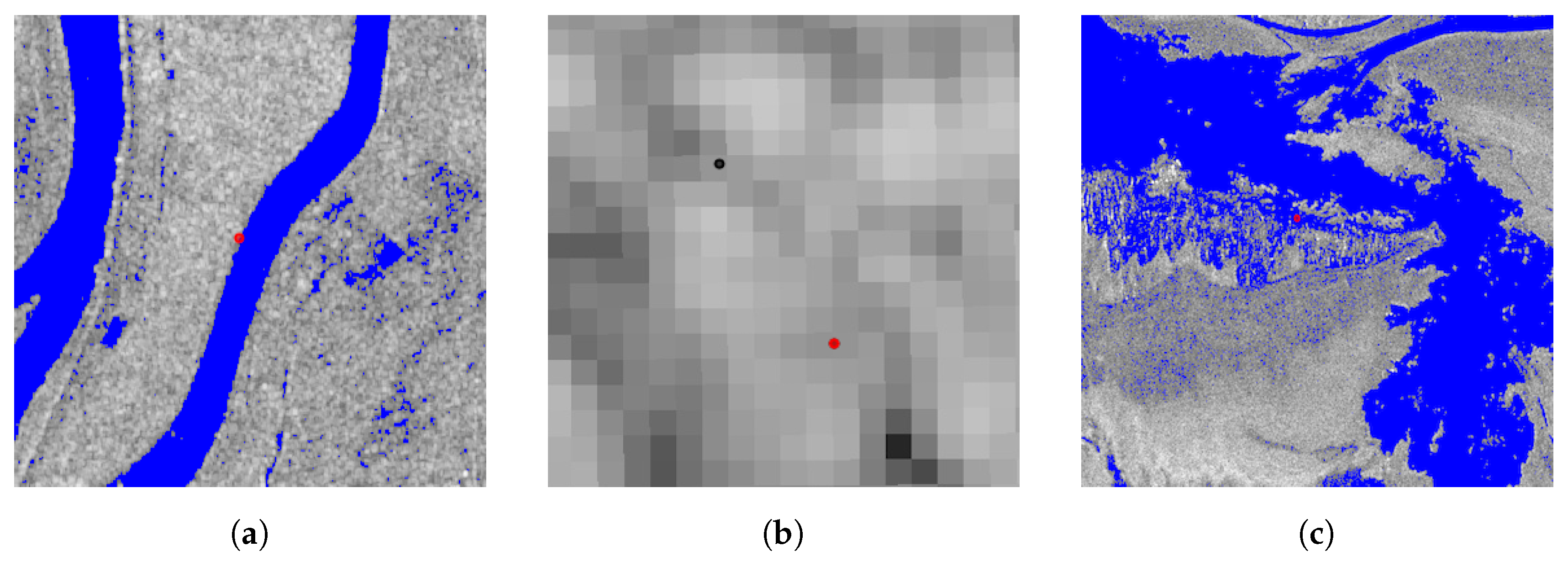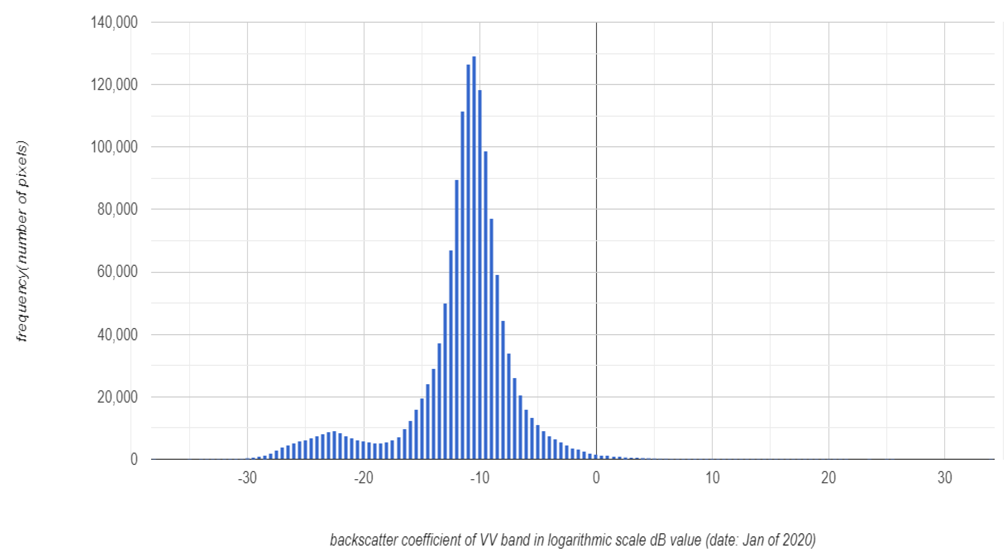With the help of high-performance computing and network systems, Google Earth Engine (GEE) allows online processing and analysis of radar imagery by writing light-weight scripts with a Google account, speeding the process in a cloud-based platform [21]. The plethora of data catalogs and innovative processing algorithms provided by GEE can effectively eliminate the barriers caused by the traditional platforms. The water detection algorithms based on radar sensors have emerged in several categories: thresholding, classification and object-based image analysis. In general, thresholding has commonly been adopted to discriminate water from nonwater surface in the logarithmic representation of the radar imagery, where the water and nonwater features are shown as two Gaussian distributions in the histogram of backscatter coefficient of radar data in dB scale. Although it is limited by double bounce scattering issues because waters beneath vegetation layers may cause extra radar backscatter [22], thresholding is still an efficient and simple method for water extraction of rural areas in winter season with less complicated vegetation coverage.

One classical method to select the threshold is to manually pick the smallest valley values between the two peaks of distributions based upon visual inspection by the researcher. The main issue of this method is the bias caused by each individual observer. The solution to offset the researcher’s observation bias is to apply computer programming to select a less biased lowest point in the valley, which can be computationally efficient in linear time. However, the intensity histogram presented by radar imaging may not necessarily provide a sharp valley but usually a flat region between the peaks. Thus, it will be less accurate or reasonable to pick the smallest valley value in this case, as the value of the selected point may deviate slightly from the value of its neighboring points in the open intervals next to the selected point. Furthermore, due to the noise in radar detection, the strict convex property is not guaranteed in the valley region between the two peaks. In other words, there may exist multiple local peaks and minimums which are close to each other. In this case, the method of picking the smallest valley value is badly influenced by the noise.

The Gaussian Mixture Model is another conventional method for binary classification based on distribution. The distribution of water and nonwater objects in the radar intensity (dB) histogram presents approximately as two Gaussian Distributions with separate means ${\mu }_1$ and ${\mu }_2$ and standard deviations ${\sigma }_1$ and ${\sigma }_2$ [23]. One of the distributions is the conditional probability of the dB value of the water pixels while the other is the conditional probability of the dB value of the nonwater pixels. The objective of this model is to maximize conditional probability of the prediction $\widehat{y}$ given any dB values (x). According to the Bayes Theorem, this equates to maximizing the multiplication of the conditional probability of x over $\widehat{y}$ and the marginal probability of $\widehat{y}$.

However, the issue with such formulation of the problem is based on the assumption of the prior distribution of water and land as a Gaussian Distribution. However, such an assumption cannot be directly assumed to be correct for universal cases. Moreover, the distribution parameters ${\mu }_1$, ${\sigma }_1$, ${\mu }_2$, ${\sigma }_2$ are unknowns. The researcher also needs to identify estimators for these four parameters through the density diagram. Possible solutions for estimation of these unknown parameters can be iterative methods such as Expectation Maximization Method [24], however, it is unstable for two reasons. First, the iteration process is time consuming to reach a satisfied accuracy. Second, it is also likely to be constrained in some local optimum points and thus never reaches global optimal solution [25].

Instead, we propose to use the Otsu Method to solve this thresholding problem. The Otsu Method is an unsupervised method and it was initially designed to select a threshold to separate an object out of its background, through the gray-level histogram of the image [25]. In application, the Otsu Method can be widely extended to work on other density histograms or distributions other than gray-level histogram from images and can also be applied for multi-thresholding problems. The Otsu Method is a better approach for this problem as compared to some conventional solutions because it automatically selects a threshold from two mixed distributions through the density histogram [25]. In addition, the Otsu Method does not require prior knowledge nor assumptions of the distribution of objects [25]. Furthermore, the Otsu Method is equivalent to the K-Means Method but the Otsu Method can provide the global optimal solution, while K - Means Method may be limited to the local optimum point [26]. Although it is computationally complex and heavy because of iterative searching [26], GEE can speed up the Otsu Method with its cloud computing platform. For instance, the Otsu Method has been applied on the cloud-free Landsat TM images for urban land cover detection, which focused on differentiating the urban land and nonurban land region in Haidian District of Beijing, China [27]. This research resulted in an accuracy of $84.83\%$ for the Otsu Method, which was larger than the accuracy of $74\%$ for the conventional postclassification change detection method [27]. Another study used the Otsu Method on the SAR data for the detection of oil spills over sea surfaces, which tried to find a threshold on the radar data to draw the edge of spilled oil film floating over the sea [28]. It examined the Penglai oil field and the Gulf of Dalian, resulting in an error rate of $3.0\%$ on the Penglai oil field and an error rate of $13.0\%$ on the Gulf of Dalian for the Otsu Method [28]. Even though the Otsu Method has already been widely applied in thresholding problems, it has been seldom used for surface water extraction. Furthermore, most previous studies do not provide algorithms and detailed scripts for implementation of the Otsu Method. Thus, we were interested in the application of the Otsu Method for surface water detection and providing reusable code for future implementation.

Therefore, the objectives of the present work are to:

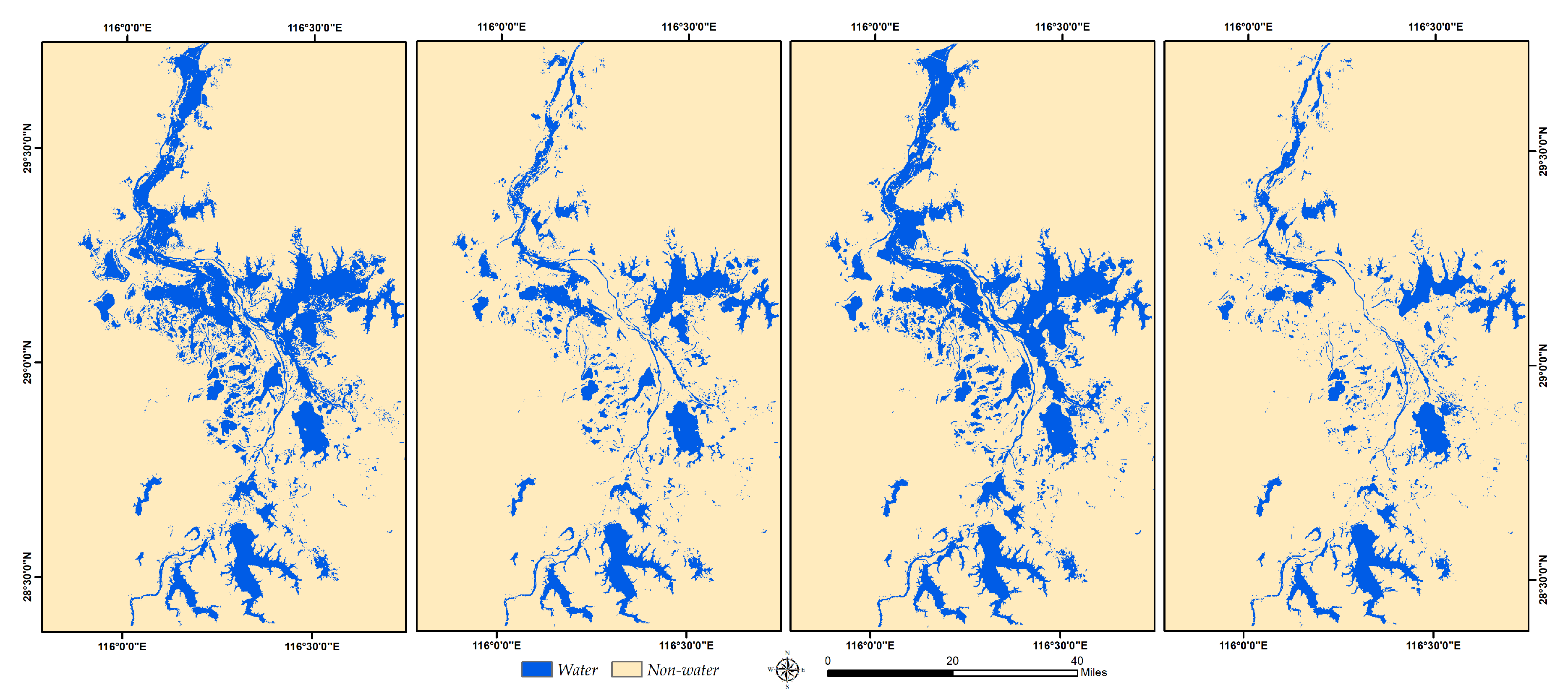
• Implement the Otsu Method and write reusable scripts to automatically select thresholds for surface water extraction using Sentinel-1 data on Google Earth Engine
• Analyze the advantages and disadvantages of an unsupervised classifier from both mathematical and application perspectives
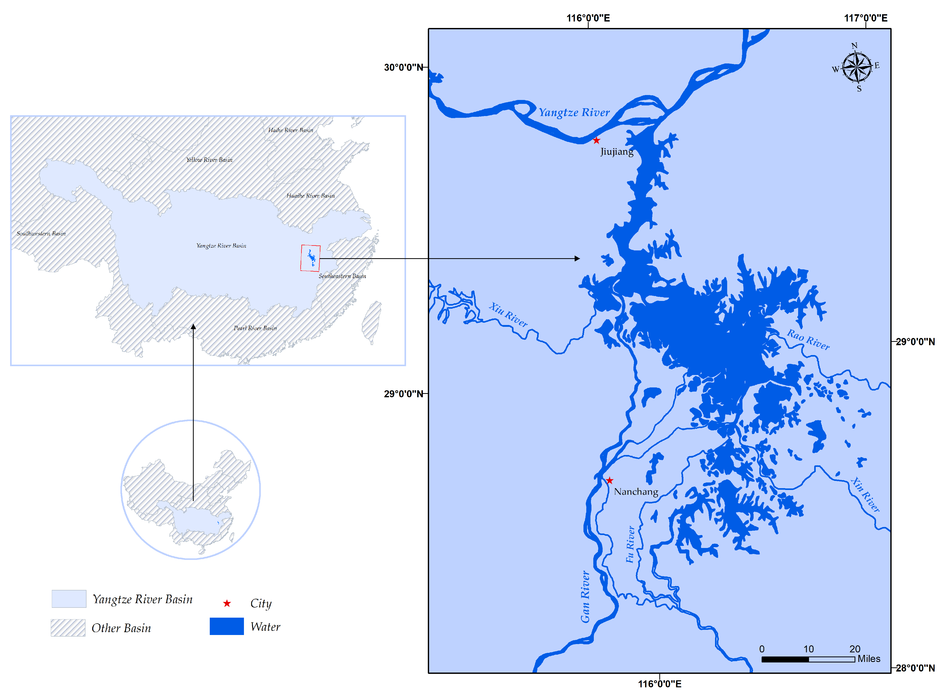
• Contribute to the knowledge base of hydrological variation at Poyang lake by mapping surface water extent of the lake in January 2017, 2018, 2019 and 2020

2. Materials and Methods

2.1. Study Area

Poyang lake, the largest freshwater lake in China, is located between Nanchang City and Jiujiang City, to the north of Jiangxi Province. The basin crosses from ${28}^{\circ }{22}^{\prime }$ to ${29}^{\circ }{45}^{\prime }$ N and ${115}^{\circ }{47}^{\prime }$ to ${116}^{\circ }{45}^{\prime }$ E, which belongs to a humid, subtropical monsoon climate zone, with an average annual temperature of 17.5 °C and average annual precipitation of 1665 mm [29]. Poyang lake basin is fed by the Xiu, Gan, Fu, Xin and Rao rivers, while the basin connects to the Yangtze river through an outflow channel at the north end of the lake (Figure 1). The lake has a surface area of approximately 4000 square kilometers at its summer high-water level [30,31]. Beyond its size, Poyang lake is also significant for several economic and ecological reasons. For instance, Poyang lake’s aquatic ecosystems are wintering home to thousands of migratory waterbirds, including the Siberian crane—a critically endangered species whose 4000 surviving individuals spend their winters almost solely in the wetlands around Poyang lake [32]. However, Poyang lake has undergone a series of significant transformations that threaten the variability and critical habitats in the region. While surface water areas have traditionally fluctuated on a seasonal scale—peaking in the summer and receding in the winter—large interannual declines in mean water level have been observed in recent years [33]. The substantial variations of the surface water area and dramatic seasonal water level fluctuations of 8 to 22 m each year are caused by the regional hydrological regime, which is controlled both by the five catchment rivers and the Yangtze River [34]. Additionally, groundwater dynamics are highly affected by the variations in the lake water level, rather than local precipitation, indicating a close hydraulic relationship between groundwater and the lake [35].

2.2. Platform and Data

Google Earth Engine (GEE, https://earthengine.google.com) consists of a multipetabyte satellite imagery data catalog colocated with a high-performance, intrinsically parallel cloud computation service. Users can access GEE through an Internet-accessible application programming interface (API) and an associated web-based interactive development environment (IDE) that enables rapid prototyping and visualization of results. This cloud computing platform not only makes it easy to access most of the geospatial datasets but also enables high throughput analysis. There are many examples where environmental scientists empowered their research with help of GEE, such as population mapping [36], cropland mapping [37], extraction of glacial lakes [38] and probabilistic wetland mapping [39].

Sentinel-1 is the first Copernicus Program satellite constellation deployed by the European Space Agency. This space mission is composed of two satellites, Sentinel-1A and Sentinel-1B, carrying a C-band synthetic-aperture radar instrument which collects data in all weather, day or night [40]. Since radar sensors have the advantage in detecting moisture and water because of their ability to penetrate clouds, Sentinel-1 is one of the most common datasets for surface water detection [41] and flood mapping [42].

The winter low-water season of Poyang lake provides important foraging habitat and wintering area for many waterbirds of special concern, including the critically endangered Siberian crane. Because of the importance of water level during this time, we looked at images taken in January over subsequent years. We loaded Sentinel-1 Level-1 IW GRD images from the data catalog of GEE from January 2017–2020 (

Table 1. Data Collection for Inundation Area Detection.

Platform	Type	Spatial Resolution	Date	Band	Instrument	Orbit
Sentinel 1 B	GRD	10 m	4 January 2020	VV	IW	19666
Sentinel 1 B	GRD	10 m	9 January 2019	VV	IW	14416
Sentinel 1 B	GRD	10 m	2 January 2018	VV	IW	8991
Sentinel 1 B	GRD	10 m	7 January 2017	VV	IW	3741

). The imagery acquired on January of 2020 was used to evaluate our Otsu Method implementation on GEE. The others were used to analyze the water area change in January across 4 years from 2017 to 2020.

2.3. Otsu Method

In this section, we firstly introduce the main idea of the Otsu Method [25,26] in a general framework and then we discuss how the Otsu Method is applied on this thresholding problem with a radar value density histogram.

Here we use the following notations:

• set C is the index set of all elements.
• i is the index of i-th element, where $i\in C$ refers to i-th element belonging to the whole set C we are considering. $x_i$ is the value for this i-th element and without loss of generality, we can assume that $x_i$ are sorted. Explicitly, $x_i<x_j$, if $i<j$, for $i,j\in C$.
• $p_i$ is the probability or density of the element i. It is clear that ${\displaystyle \sum _{i\in C}}{p}_i=1$.
• we try to split up the set C into two disjoint subclusters of index $C_0$, $C_1$, where $C_0,C_1\subset C$ and $C_0{\displaystyle \dot{\bigcup }}{C}_1=C$.
• ${\mu }_j$ is the center or the mean value of cluster $C_j$, for $j=0,1$:

  $${\mu }_j=\frac{{\displaystyle \sum _{i\in C_j}}{p}_i·x_i}{{\displaystyle \sum _{i\in C_j}}{p}_i}, \mathrm{for} j=0,1$$
• $\mu$ is the center or the mean value of the whole set C:

  $$\mu =\sum _{i\in C}{p}_i·x_i=\sum _{i\in C_0{\displaystyle \dot{\bigcup }}{C}_1}{p}_i·x_i$$
• $V_j$ is denoted as the inner-variance of the cluster $C_j$, which is defined as the weighted summation of the squared distance of cluster $C_j$’s each data point from its center ${\mu }_j$, for $j=0,1$:

  $$V_j=\sum _{i\in C_j}{p}_i·{(x_i-{\mu }_j)}^2, \mathrm{for} j=0,1$$
• $V_{0,1}$ is denoted as the interclass variance between the cluster $C_0$ and cluster $C_1$ [25], which is defined as the weighted summation of the squared distance of each cluster’s center ${\mu }_j$ from the center of the whole set $\mu$:

  $$V_{0,1}=\sum _{j=0,1}((\sum _{i\in C_j}{p}_i)·{({\mu }_j-\mu )}^2)$$
• V is denoted as the total-variance, which is defined as the weighted summation of the squared distance of all data points from the center of the whole set $\mu$. Furthermore, we can see that V is actually exactly the variance ${\sigma }_C^2$ of the set C:

  $$V=\sum _{i\in C}{p}_i·{(x_i-\mu )}^2$$

The main idea of the Otsu Method is to minimize the summation of the inner-variance $V_j$ of all clusters $C_j$, which is called intraclass variance [25]. The inner-variance of a cluster shows the summation of squared distance of each element to the center of the cluster as we defined, and the smaller value of the inner-variance presents the closer distance of each point toward the center of the cluster, which shows a closer relationship or higher similarity that the elements in this cluster share. Therefore, the best separation of the whole set of elements should group the similar elements in the same cluster as optimally as possible. In mathematics, this is equivalent to minimizing the summation of inner-variance inside each cluster. The objective function is formulated as follows:

$$\underset{C_0,C_1}{min}\sum _{j=0,1}{V}_j=\underset{C_0,C_1}{min}\sum _{j=0,1}\sum _{i\in C_j}{p}_i·{(x_i-{\mu }_j)}^2$$

(1)

Furthermore, the summation of each cluster’s inner-variance and the interclass variance should be equal to the total-variance of the whole set [25], which is a constant for a fixed data set.

$$V=\sum _{j=0,1}{V}_j+V_{0,1}$$

(2)

Therefore, the previous objective function Equation (1) is equivalent to maximizing the interclass variance $V_{0,1}$:

$$\underset{C_0,C_1}{max}\sum _{j=0,1}((\sum _{i\in C_j}{p}_i)·{({\mu }_j-\mu )}^2)$$

(3)

Now, in applying the Otsu Method on the density histogram, we can have:

• The set of all possible bin’s values on the density histogram as $\Theta$, which is also the hypothesis space for the estimation of the threshold.
• The density corresponding to the bin with value $\theta$ is denoted as $p_{\theta }$ and we should have $1={\displaystyle \sum _{\theta \in \Theta }}{p}_{\theta }$.
• For each bin value $\theta \in \Theta$, we can put a corresponding index $i_{\theta }$ into the indexed set C, where $i_{\theta }$-th bin on the density histogram has a bin value of $\theta$. Therefore, $x_{i_{\theta }}=\theta$ and $p_{i_{\theta }}$ is equal to the density $p_{\theta }$ of the bin with value $\theta$ from the density histogram.
• The final prediction of the threshold is denoted as $\widehat{\theta }\in \Theta$, which corresponds to the index $i_{\widehat{\theta }}\in C$.
• the two separate clusters formed by a threshold $\theta$ is $C_0=\{i:i<i_{\theta },i\in C\}$ and $C_1=\{i:i\ge i_{\theta },i\in C\}$.

The final estimation of the threshold $\widehat{\theta }$ should be the one based on which the subcluster $C_0^{*}$ and $C_1^{*}$ can reach the optimal value of the objective function in Equation (3). Then, we can have:

$$i_{\widehat{\theta }}={\displaystyle \underset{i\in C_1^{*}}{min}}i$$

(4)

$$\widehat{\theta }=x_{i_{\widehat{\theta }}}$$

(5)

This optimization problem can be solved in at most quadratic polynomial time of the size of the finite set $\Theta$, i.e., the time complexity will be $O(|\Theta {|}^2)$. One possible implementation as shown in Algorithm 1 is to iterate through the finite set and record the element in the set that provides the highest value for the objective function. Each inner iteration takes linear time to calculate the objective function.

Algorithm 1: OtsuMethodFindOptimalThresholding (Time: $O(|\Theta {|}^2)$)

We can further improve the time complexity of the Otsu Method into linear time complexity of $O(|\Theta |)$. If we store the value of ${\mu }_0$ and ${\mu }_1$ from previous outer loop iteration, then it will take constant time $O(1)$ for recomputing the objective function value based on the Equation (3) for the newly updated $C_0$ and $C_1$ in this current round.

Because the Otsu Method iterates through all the possible values for the threshold and compares the objective values with all these possible thresholds, the implementation of Otsu Method in Algorithm 1 provides a global optimal solution for the objective function in Equation (3).

2.4. Water Detection

Once the preprocessing procedure was completed by GEE, the histogram of VV band was generated, and the Otsu method was used to search over the thresholds that are represented by the bins in the histogram. The optimal threshold was computed to classify the data, where the partition whose values are smaller than the threshold are labeled as water while the partition whose values are larger than the threshold are labeled as nonwater. In order to reduce the effect of double bounce scattering issues, we defined the label of water as purely open water area, while the label of nonwater included the submerged and emergent aquatic vegetation and land features. The specific implementation of the Otsu Method can be found through the link: source code for the Otsu Method (by Sulong Zhou). The postprocessing procedure that removes noise and improves the quality of the classified output involving mask extraction, majority filtering and boundary clean was carried out in ArcGIS to remove the water bodies not geographically related to Poyang lake, small islands of pixels and odd edge of clusters.

2.5. Accuracy Assessment

We denote a point x with its true label y drawn from the true distribution $\mathcal{D}$ as $(x,y)\sim \mathcal{D}$, where the true distribution $\mathcal{D}$ is actually unknown. Specifically, x is the radar dB value for a pixel and defined as:

$$y=\left\{\begin{array}{cc}1\hfill & ,\mathrm{if} \mathrm{the} \mathrm{true} \mathrm{label} \mathrm{of} x \mathrm{is} \mathrm{Water}\hfill \\ 0\hfill & ,\mathrm{if} \mathrm{the} \mathrm{true} \mathrm{label} \mathrm{of} x \mathrm{is} \mathrm{Non}-\mathrm{Water}\hfill \end{array}\right.$$

Based on the estimation of the optimal threshold $\widehat{\theta }$ from the Otsu Method, we can provide the prediction of the label $\widehat{y}$ for point x as:

$$\widehat{y}=f_{\widehat{\theta }}(x)={𝟙}_{x<\widehat{\theta }}$$

(6)

where,

$${𝟙}_{x<\widehat{\theta }}=\left\{\begin{array}{cc}1\hfill & ,\mathrm{if} x<\widehat{\theta }\hfill \\ 0\hfill & ,\mathrm{otherwise}\hfill \end{array}\right.$$

Accuracy measures the agreement between a standard assumed to be correct and a classified image of unknown quality [43]. Classification errors occur when a pixel (or feature) belonging to one category is assigned to another category. Errors of omission occur when a feature is left out of the category being evaluated; errors of commission occur when a feature is incorrectly included in the category being evaluated [44]. An error of omission in one category will be counted as an error in commission in another category. Explicitly, for a pixel’s dB value x and its true label y from the unknown true distribution $\mathcal{D}$, the error happens when $\widehat{y}\ne y$. Therefore, accuracy can be mathematically defined as the follow:

$$Accuracy={\mathbb{E}}_{(x,y)\sim \mathcal{D}}{𝟙}_{\widehat{y}=y}$$

(7)

Since the true distribution $\mathcal{D}$ is unknown, it is not possible to calculate the accuracy through Equation (7). Therefore, we need an estimator to estimate such accuracy. One possible way to estimate is based on the Empirical Distribution [45]. A test set $T={\left\{(x_i,y_i)\right\}}_{i=1}^n$, which forms an empirical distribution $\widehat{D}$, is used to approximate the true distribution $\mathcal{D}$, where each element $(x_i,y_i)$ is independently and identically (i.i.d) drawn from the true distribution $\mathcal{D}$.

$${\left\{(x_i,y_i)\right\}}_{i=1}^n\stackrel{i.i.d}{\sim }\mathcal{D}$$

The empirical estimator of accuracy $\widehat{Accuracy}$ for classification function $f_{\widehat{\theta }}$ can be expressed as:

$$\widehat{Accuracy}=\frac{1}{n}·{\displaystyle \sum _{(x_i,y_i)\in T}}{𝟙}_{{\widehat{y}}_i=y_i},where{\widehat{y}}_i=f_{\widehat{\theta }}(x_i)$$

(8)

Since $(x_i,y_i)\in T$, for $\forall i=1,\dots ,n$, is $i.i.d$ drawn from the true distribution $\mathcal{D}$, this estimator $\widehat{Accuracy}$ in Equation (8) is an unbiased estimator of the true $Accuracy$ as defined in Equation (7) [46], proved as follows:

Proof of Unbias Estimator. 

$$\begin{array}{cc}\hfill \mathbb{E}[\widehat{Accuracy}]& =\mathbb{E}[\frac{1}{n}·{\displaystyle \sum _{(x_i,y_i)\in T}}{𝟙}_{{\widehat{y}}_i=y_i}]\hfill \\ \hfill & =\frac{1}{n}·{\displaystyle \sum _{(x_i,y_i)\in T}}\mathbb{E}[{𝟙}_{{\widehat{y}}_i=y_i}]\hfill \\ \hfill & \stackrel{i.i.d}{=}\frac{1}{n}·{\displaystyle \sum _{(x_i,y_i)\in T}}{\mathbb{E}}_{(x,y)\sim \mathcal{D}}[{𝟙}_{\widehat{y}=y}]\hfill \\ \hfill & =\frac{1}{n}·n·{\mathbb{E}}_{(x,y)\sim \mathcal{D}}[{𝟙}_{\widehat{y}=y}]\hfill \\ \hfill & ={\mathbb{E}}_{(x,y)\sim \mathcal{D}}[{𝟙}_{\widehat{y}=y}]\hfill \\ \hfill & =Accuracy\hfill \end{array}$$

 □

A modified double-blind visual assessment of a random sample of test sites was used to assess classification accuracy. Firstly, a random set of 304 test sites was generated across the region, and the algorithm can be found through the link: source code for random points (by Sulong Zhou). This random set corresponds to the test set T with $n=304$ and each element $(x_i,y_i)$ is $i.i.d$ drawn from the true distribution $\mathcal{D}$, which is the distribution of dB value and label of the locations in the study area as shown in Figure 1. Next, it was assigned to a team in Nanchang who visited all accessible points from the set of 304. Then based on their experience, knowledge, and observation in both real field settings and Google Earth, they distinguished the visited sites and labeled them as water and nonwater areas. We finally verified the ground truth data by comparison with false color composite Landsat 8 imagery, and rectified 19 labels. Explicitly, this step is to assess the true label $y_i$ as water or nonwater for each $x_i$ in the test set T. Finally, these labeled test sites ${\left\{(x_i,y_i,{\widehat{y}}_i)\right\}}_{i=1}^{n=304}$, where ${\widehat{y}}_i=f_{\widehat{\theta }}(x_i)$, were input as the ground truth information to generate a confusion matrix.

3. Results and Discussion

3.1. Confusion Matrix

The overall accuracy before test set rectification was $83.88\%$ (

Table 2. Confusion Matrix Before Test Set Rectification.

		Predicted Label
		Water	Nonwater	Total
Actual Label	Water	53	40	93
	Nonwater	9	202	211
	Total	62	242	304

) while the overall accuracy after test set rectification increased to $92.11\%$ (

Table 3. Confusion Matrix After Test Set Rectification.

		Predicted Label
		Water	Nonwater	Total
Actual Label	Water	75	18	93
	Nonwater	6	205	211
	Total	81	223	304

). The diagonal elements (left to right, top to bottom) in the matrix represent the number of correctly classified pixels of each class, for example, the number of ground truth pixels with a label of water that was actually predicted as water during classification.

In contrast, the cross-diagonal elements represent misclassified pixels. A large loss of accuracy (40 out of 93) occurs at the pixels that are water in ground truth data but are classified into nonwater (Figure 2a). This happens for two reasons. First, many of these points are located at boundary pixels between two classes. Second, most points are isolated from their neighbor clusters. The boundary area has the mixed pixels problem which means both water and nonwater contribute to the observed spectral response of the pixel. In addition, the penetrating ability of C-band is unable to detect water hidden below rocks or vegetation cover where the normalized difference vegetation index (NDVI) is greater than $0.7$ [47]. By contrast, there are only nine pixels that are misclassified into water while they are labeled as nonwater in ground truth data (Figure 2c). This is likely because the VV band can be affected by wind so that the wavy water surface will be classified into nonwater because of the diffuse refection. On the other hand, we examined each of those misclassified points and discovered that human errors in test data also compromise the overall accuracy. Twenty-two out of 40 nonwater test points and three out of nine water test points were rectified by using Landsat 8 imagery as a reference. As a result, the overall accuracy increased nearly $9\%$.

Note that the rectification of the test set T does not influence the training process nor the estimation of the optimal threshold $\widehat{\theta }$ provided by the Otsu Method. Since the Otsu Method is an unsupervised learning algorithm, it does not depend on the label y of data for its training process. This property presents the feature of data corruption tolerance of the Otsu Method. In other words, corruption in the input data’s label does not influence the actual training or performance of the Otsu Method. In addition, the test set T is only used for the statistical estimation or evaluation for the performance of the classification based on the estimation of optimal threshold $\widehat{\theta }$ from the Otsu Method.

Furthermore, for factors influencing the accuracy, it is worth noting that the radar dB value with its corresponding label is linear nonseparable data [48]. In other words, there does not exist a hyperplane to clearly separate the dB value corresponding to the label of Water and the dB value corresponding to Nonwater. Because there exists two different regions or pixels i and j, where $i\ne j$, such that they have the same dB value $x_i=x_j$, but they are actually having different label $y_i\ne y_j$, one region corresponds to water and another region corresponds to nonwater. Such linear nonseparability may decrease the accuracy of this learning algorithm, which is unavoidable because the Otsu Method is trying to use a linear threshold to separate the data. One possible example of such region i and j is shown in the Figure 2b.

3.2. Water Area

The optimal threshold for 2020 was selected as $-16.87$ through the histogram, where the low peak corresponded to water pixels while the high peak corresponded to nonwater pixels (see Figure 3). Similarly, the optimal thresholds for each year from 2017 to 2019 were $-14.88$, $-16.93$ and $-16.96$ respectively. Based on the auto-selected thresholds derived from the Otsu Method, the imagery was classified into water and nonwater regions. As a result, the surface water acreages of Poyang lake from 2017 to 2020 were obtained and are presented in

Table 4. Area (km${}^2$) of Poyang lake from 2017 to 2020.

Year	Area (km${}^2$)
2017	1959.50
2018	1308.67
2019	1948.72
2020	1092.82

and visualized from left to right in the Figure 4. The surface water area decreased by nearly 650 km${}^2$ between 2017 and 2018, then increased by nearly 640 km${}^2$ between 2018 and 2019 and finally decreased by nearly 856 km${}^2$ between 2019 and 2020. This shows that surface water area of Poyang lake decreased with fluctuation, which is consistent with other research on variation of the surface water of Poyang lake during the time period of 1988–2016 [49].

In addition to the significant interannual variation, our results also showed the spatial variation of surface water area. The dry or draw down areas mainly occurred in the center and the boundary of the lake at the same time. The water areas located to the north (connected to Yangtze River) and west (connected to Gan River) accounted for most of the variation, while the water areas located at the east and south maintained much less variation.

The water area variations typically are closely associated to water level variations in Poyang lake basin [50]. Both water area and water level are dominant factors for wetlands in Poyang lake, and thus affect habitat distribution and accessibility. In this case, our classification results that show the spatiotemporal water area variations can provide robust linkages to habitat availability and suggest future research to further quantify this relationship.

4. Conclusions

Through this research we mapped the spatio-temporal variation of Poyang lake in January from 2017 to 2020 and showed that the surface water area fluctuated annually and tended to shrink both in the center and boundary of the lake over the past four years. The variation was consistent with related Poyang lake research for earlier decades. Our mapping approach involved a novel implementation of the Otsu Method and processing of Sentinel-1 data in Google Earth Engine. GEE performed well as a powerful cloud computing platform to implement an exhaustive searching algorithm. We provided detailed mathematical explanation to enumerate the advantages and limitations of the Otsu Method that were not clearly indicated in previous remote sensing research. We also demonstrated that the Otsu Method can be an effective classifier for threshold auto-selected algorithms to extract water surface with use of Sentinel-1 data. As a result, the Otsu Method has potential to be applied to other water related studies, such as water extraction applications for other lake regions, water pollutant detection for environmental assessment and aquatic habitat mapping for ecological conservation, using the open access scripts of the threshold algorithm contributed here.

In the future, to reduce the influence of linear nonseparability nature of the data, the 2D Otsu Method [51] can be applied. However, since the Otsu Method is an unsupervised method, we have not compared its performance with supervised learning algorithms. The supervised learning algorithm requires training data that is unavailable for the January of 2020 at this time. In addition, the Otsu Method is affected by the penetration ability of single C-band radar signal so that it is difficult to capture water beneath the vegetation. To advance our research toward mapping aquatic habitat availability, we recommend the comparison between supervised and unsupervised methods by using different series of imagery to discriminate vegetation zones. This next step will allow us to identify and project the spatial distribution of available foraging habitat under varying hydrological conditions for species of concern like Siberian crane and other aquatic organisms.

References

1. Pekel, J.F.; Cottam, A.; Gorelick, N.; Belward, A.S. High-resolution mapping of global surface water and its long-term changes. Nature 2016, 540, 418–422. [Google Scholar] [CrossRef]
2. Downing, J.A.; Prairie, Y.; Cole, J.; Duarte, C.; Tranvik, L.; Striegl, R.G.; McDowell, W.; Kortelainen, P.; Caraco, N.; Melack, J.; et al. The global abundance and size distribution of lakes, ponds, and impoundments. Limnol. Oceanogr. 2006, 51, 2388–2397. [Google Scholar] [CrossRef] [Green Version]
3. Barrow, C.J. Water Resources and Agricultural Development in the Tropics; Routledge: London, UK; New York, NY, USA, 2016. [Google Scholar]
4. Song, J.H.; Kang, M.S.; Song, I.; Jun, S.M. Water balance in irrigation reservoirs considering flood control and irrigation efficiency variation. J. Irriga. Drain. Eng. 2016, 142, 04016003. [Google Scholar] [CrossRef]
5. Huang, Z.; Lu, L.; Jiao, G.; Jiang, J.; Ye, Q. Analysis of the correlations between environmental factors and rare cranes in the Poyang lake region of China. J. Great Lakes Res. 2018, 44, 140–148. [Google Scholar] [CrossRef]
6. Prigent, C.; Papa, F.; Aires, F.; Jimenez, C.; Rossow, W.; Matthews, E. Changes in land surface water dynamics since the 1990s and relation to population pressure. Geophys. Res. Lett. 2012, 39. [Google Scholar] [CrossRef] [Green Version]
7. Holgerson, M.A.; Raymond, P.A. Large contribution to inland water CO2 and CH4 emissions from very small ponds. Nat. Geosci. 2016, 9, 222–226. [Google Scholar] [CrossRef]
8. Gardner, R.C.; Barchiesi, S.; Beltrame, C.; Finlayson, C.; Galewski, T.; Harrison, I.; Paganini, M.; Perennou, C.; Pritchard, D.; Rosenqvist, A.; et al. State of the World’s Wetlands and Their Services to People: A Compilation of Recent Analyses; Ramsar Briefing Note No. 7; Ramsar Convention Secretariat: Gland, Switzerland, 2015. [Google Scholar] [CrossRef] [Green Version]
9. De Amorim, W.S.; Valduga, I.B.; Ribeiro, J.M.P.; Williamson, V.G.; Krauser, G.E.; Magtoto, M.K.; de Andrade, J.B.S.O. The nexus between water, energy, and food in the context of the global risks: An analysis of the interactions between food, water, and energy security. Environ. Impact Assess. Rev. 2018, 72, 1–11. [Google Scholar] [CrossRef]
10. Vörösmarty, C.J.; Green, P.; Salisbury, J.; Lammers, R.B. Global water resources: Vulnerability from climate change and population growth. Science 2000, 289, 284–288. [Google Scholar] [CrossRef] [PubMed] [Green Version]
11. Van Dijk, A.I.; Beck, H.E.; Crosbie, R.S.; de Jeu, R.A.; Liu, Y.Y.; Podger, G.M.; Timbal, B.; Viney, N.R. The Millennium Drought in southeast Australia (2001–2009): Natural and human causes and implications for water resources, ecosystems, economy, and society. Water Resour. Res. 2013, 49, 1040–1057. [Google Scholar] [CrossRef]
12. Hipsey, M.R.; Bruce, L.C.; Boon, C.; Busch, B.; Carey, C.C.; Hamilton, D.P.; Hanson, P.C.; Read, J.S.; De Sousa, E.; Weber, M.; et al. A General Lake Model (GLM 3.0) for linking with high-frequency sensor data from the Global Lake Ecological Observatory Network (GLEON). Geosci. Model Dev. 2019, 12, 473–523. [Google Scholar] [CrossRef] [Green Version]
13. Campbell, J.B.; Wynne, R.H. Introduction to Remote Sensing; Guilford Press: New York, NY, USA, 2011. [Google Scholar]
14. Sun, G.; Chen, X.; Ren, J.; Zhang, A.; Jia, X. Stratified spectral mixture analysis of medium resolution imagery for impervious surface mapping. Int. J. Appl. Earth Obs. Geoinf. 2017, 60, 38–48. [Google Scholar] [CrossRef] [Green Version]
15. Busetto, L.; Meroni, M.; Colombo, R. Combining medium and coarse spatial resolution satellite data to improve the estimation of sub-pixel NDVI time series. Remote Sens. Environ. 2008, 112, 118–131. [Google Scholar] [CrossRef]
16. Woodcock, C.E.; Allen, R.; Anderson, M.; Belward, A.; Bindschadler, R.; Cohen, W.; Gao, F.; Goward, S.N.; Helder, D.; Helmer, E.; et al. Free access to Landsat imagery. Science 2008, 320, 1011. [Google Scholar] [CrossRef]
17. Joshi, N.; Baumann, M.; Ehammer, A.; Fensholt, R.; Grogan, K.; Hostert, P.; Jepsen, M.R.; Kuemmerle, T.; Meyfroidt, P.; Mitchard, E.T.; et al. A review of the application of optical and radar remote sensing data fusion to land use mapping and monitoring. Remote Sens. 2016, 8, 70. [Google Scholar] [CrossRef] [Green Version]
18. Bioresita, F.; Puissant, A.; Stumpf, A.; Malet, J.P. A method for automatic and rapid mapping of water surfaces from sentinel-1 imagery. Remote Sens. 2018, 10, 217. [Google Scholar] [CrossRef] [Green Version]
19. Twele, A.; Cao, W.; Plank, S.; Martinis, S. Sentinel-1-based flood mapping: A fully automated processing chain. Int. J. Remote Sens. 2016, 37, 2990–3004. [Google Scholar] [CrossRef]
20. Ye, Y.; Bruzzone, L.; Shan, J.; Bovolo, F.; Zhu, Q. A Fast and Robust Matching Framework for Multimodal Remote Sensing Image Registration. arXiv 2018, arXiv:1808.06194. [Google Scholar]
21. Gorelick, N.; Hancher, M.; Dixon, M.; Ilyushchenko, S.; Thau, D.; Moore, R. Google Earth Engine: Planetary-scale geospatial analysis for everyone. Remote Sens. Environ. 2017, 202, 18–27. [Google Scholar] [CrossRef]
22. Schumann, G.J.P.; Moller, D.K. Microwave remote sensing of flood inundation. Phys. Chem. Earth Parts A B C 2015, 83, 84–95. [Google Scholar] [CrossRef]
23. Xing, L.; Tang, X.; Wang, H.; Fan, W.; Wang, G. Monitoring monthly surface water dynamics of Dongting Lake using Sentinel-1 data at 10 m. PeerJ 2018, 6, e4992. [Google Scholar] [CrossRef]
24. Wolynetz, M. Algorithm AS 138: Maximum likelihood estimation from confined and censored normal data. J. R. Stat. Soc. Ser. C Appl. Stat. 1979, 28, 185–195. [Google Scholar] [CrossRef]
25. Otsu, N. A threshold selection method from gray-level histograms. IEEE Trans. Syst. Man Cybern. 1979, 9, 62–66. [Google Scholar] [CrossRef] [Green Version]
26. Vala, H.J.; Baxi, A. A review on Otsu image segmentation algorithm. Int. J. Adv. Res. Comput. Eng. Technol. IJARCET 2013, 2, 387–389. [Google Scholar]
27. An, K.; Zhang, J.; Xiao, Y. Object-oriented urban dynamic monitoring—A case study of Haidian district of Beijing. Chin. Geogr. Sci. 2007, 17, 236–242. [Google Scholar] [CrossRef]
28. Yu, F.; Sun, W.; Li, J.; Zhao, Y.; Zhang, Y.; Chen, G. An improved Otsu method for oil spill detection from SAR images. Oceanologia 2017, 59, 311–317. [Google Scholar] [CrossRef]
29. Ye, X.; Li, X.; Xu, C.Y.; Zhang, Q. Similarity, difference and correlation of meteorological and hydrological drought indices in a humid climate region–the Poyang lake catchment in China. Hydrol. Res. 2016, 47, 1211–1223. [Google Scholar] [CrossRef]
30. Shankman, D.; Keim, B.D.; Song, J. Flood frequency in China’s Poyang lake region: Trends and teleconnections. Int. J. Climatol. A J. R. Meteorol. Soc. 2006, 26, 1255–1266. [Google Scholar] [CrossRef] [Green Version]
31. Burnham, J.; Barzen, J.; Pidgeon, A.M.; Sun, B.; Wu, J.; Liu, G.; Jiang, H. Novel foraging by wintering Siberian Cranes Leucogeranus leucogeranus at China’s Poyang lake indicates broader changes in the ecosystem and raises new challenges for a critically endangered species. Bird Conserv. Int. 2017, 27, 204–223. [Google Scholar] [CrossRef] [Green Version]
32. Mei, X.; Dai, Z.; Fagherazzi, S.; Chen, J. Dramatic variations in emergent wetland area in China’s largest freshwater lake, Poyang lake. Adv. Water Resour. 2016, 96, 1–10. [Google Scholar] [CrossRef] [Green Version]
33. Ye, X.; Zhang, Q.; Bai, L.; Hu, Q. A modeling study of catchment discharge to Poyang lake under future climate in China. Quat. Int. 2011, 244, 221–229. [Google Scholar] [CrossRef]
34. Gao, J.H.; Jia, J.; Kettner, A.J.; Xing, F.; Wang, Y.P.; Xu, X.N.; Yang, Y.; Zou, X.Q.; Gao, S.; Qi, S.; et al. Changes in water and sediment exchange between the Changjiang River and Poyang lake under natural and anthropogenic conditions, China. Sci. Total Environ. 2014, 481, 542–553. [Google Scholar] [CrossRef] [PubMed]
35. Li, Y.; Yao, J.; Zhao, G.; Zhang, Q. Evidences of hydraulic relationships between groundwater and lake water across the large floodplain wetland of Poyang lake, China. Water Scie. Technol. Water Supply 2018, 18, 698–712. [Google Scholar] [CrossRef]
36. Patel, N.N.; Angiuli, E.; Gamba, P.; Gaughan, A.; Lisini, G.; Stevens, F.R.; Tatem, A.J.; Trianni, G. Multitemporal settlement and population mapping from Landsat using Google Earth Engine. Int. J. Appl. Earth Obs. Geoinf. 2015, 35, 199–208. [Google Scholar] [CrossRef] [Green Version]
37. Shelestov, A.; Lavreniuk, M.; Kussul, N.; Novikov, A.; Skakun, S. Exploring Google earth engine platform for big data processing: Classification of multi-temporal satellite imagery for crop mapping. Front. Earth Sci. 2017, 5, 17. [Google Scholar] [CrossRef] [Green Version]
38. Chen, F.; Zhang, M.; Tian, B.; Li, Z. Extraction of glacial lake outlines in Tibet Plateau using Landsat 8 imagery and Google Earth Engine. IEEE J. Sel. Top. Appl. Earth Obs. Remote Sens. 2017, 10, 4002–4009. [Google Scholar] [CrossRef]
39. Hird, J.N.; DeLancey, E.R.; McDermid, G.J.; Kariyeva, J. Google Earth Engine, open-access satellite data, and machine learning in support of large-area probabilistic wetland mapping. Remote Sens. 2017, 9, 1315. [Google Scholar] [CrossRef] [Green Version]
40. Torres, R.; Snoeij, P.; Geudtner, D.; Bibby, D.; Davidson, M.; Attema, E.; Potin, P.; Rommen, B.; Floury, N.; Brown, M.; et al. GMES Sentinel-1 mission. Remote Sens. Environ. 2012, 120, 9–24. [Google Scholar] [CrossRef]
41. Pham-Duc, B.; Prigent, C.; Aires, F. Surface water monitoring within Cambodia and the Vietnamese Mekong Delta over a year, with Sentinel-1 SAR observations. Water 2017, 9, 366. [Google Scholar] [CrossRef] [Green Version]
42. Borah, S.B.; Sivasankar, T.; Ramya, M.; Raju, P. Flood inundation mapping and monitoring in Kaziranga National Park, Assam using Sentinel-1 SAR data. Environ. Monit. Assess. 2018, 190, 520. [Google Scholar] [CrossRef]
43. Story, M.; Congalton, R.G. Accuracy assessment: A user’s perspective. Photogramm. Eng. Remote Sens. 1986, 52, 397–399. [Google Scholar]
44. Foody, G.M. Status of land cover classification accuracy assessment. Remote Sens. Environ. 2002, 80, 185–201. [Google Scholar] [CrossRef]
45. Goodfellow, I.; Bengio, Y.; Courville, A. Deep Learning; MIT Press: Cambridge, MA, USA, 2016. [Google Scholar]
46. Devroye, L.; Györfi, L.; Lugosi, G. A Probabilistic Theory of Pattern Recognition; Springer Science & Business Media: Berlin, Germany, 2013; Volume 31. [Google Scholar]
47. El Hajj, M.; Baghdadi, N.; Bazzi, H.; Zribi, M. Penetration analysis of SAR signals in the C and L bands for wheat, maize, and grasslands. Remote Sens. 2019, 11, 31. [Google Scholar] [CrossRef] [Green Version]
48. Friedman, J.; Hastie, T.; Tibshirani, R. The Elements of Statistical Learning; Springer Series in Statistics: New York, NY, USA, 2001; Volume 1. [Google Scholar]
49. Wang, Y.; Ma, J.; Xiao, X.; Wang, X.; Dai, S.; Zhao, B. Long-Term Dynamic of Poyang lake Surface Water: A Mapping Work Based on the Google Earth Engine Cloud Platform. Remote Sens. 2019, 11, 313. [Google Scholar] [CrossRef] [Green Version]
50. Zhang, Z.; Chen, X.; Xu, C.Y.; Hong, Y.; Hardy, J.; Sun, Z. Examining the influence of river–lake interaction on the drought and water resources in the Poyang lake basin. J. Hydrol. 2015, 522, 510–521. [Google Scholar] [CrossRef]
51. Zhang, J.; Hu, J. Image segmentation based on 2D Otsu method with histogram analysis. In Proceedings of the 2008 International Conference on Computer Science and Software Engineering, Hubei, China, 12–14 December 2008; Volume 6, pp. 105–108. [Google Scholar]
Figure 1. Location of Poyang lake within the Yangtze River Basin (left) and at an average level (right).
Ijgi 09 00424 g001
Figure 2. Three Situations of Misclassification: (a) A pixel (116.4064 E, 28.8405 N) that was misclassified into nonwater. (b) Two pixels with equal dB values but different truth label y (116.2196 E, 28.9905 N) (116.2201 E, 28.9899 N). (c) A pixel (116.1584 E, 29.2136 N) that was misclassified into water.
Ijgi 09 00424 g002
Figure 3. An Example of Histogram of VV Band in dB value (4 January 2020), the x-axis represents that backscatter coefficient is calculated in dB scale, the y-axis represents that how many pixels have the same dB value in a bin and the interval of bins is 0.5.
Ijgi 09 00424 g003
Figure 4. Inundation Area of Poyang lake in Winter of 2017, 2018, 2019 and 2020 (from left to right).
Ijgi 09 00424 g004