Multidimensional Visualization and Processing of Big Open Urban Geospatial Data on the Web


Politecnico di Milano, Department of Civil and Environmental Engineering, Piazza Leonardo da Vinci 32, 20133 Milan, Italy
*
Author to whom correspondence should be addressed.
†
Current address: European Commission, Joint Research Centre, Via Enrico Fermi 2749, 21027 Ispra, Italy.
ISPRS Int. J. Geo-Inf. 2020, 9(7), 434; https://0-doi-org.brum.beds.ac.uk/10.3390/ijgi9070434
Submission received: 6 June 2020
/
Revised: 25 June 2020
/
Accepted: 7 July 2020
/
Published: 11 July 2020
(This article belongs to the Special Issue Geodata Science and Spatial Analysis in Urban Studies)
Abstract
:The focus of this research is addressing a subset of the geovisualization (i.e., geographic visualization) challenges identified in the literature, namely multidimensional vector and raster geospatial data visualization. Moreover, the work implements an approach for multidimensional raster geospatial data processing. The results of this research are provided through a geoportal comprised of multiple applications that are related to 3D visualization of cities, ground deformation, land use and land cover and mobility. In a subset of the applications, the datasets handled are considered to be large in volume. The geospatial data were visualized on dynamic and interactive virtual globes to enable visual exploration. The geoportal is available on the web to enable cross-platform access to it. Furthermore, the geoportal was developed employing open standards, free and open source software (FOSS) and open data, most importantly to ensure interoperability and reduce the barriers to access it. The geoportal brings together various datasets, different both in terms of context and format employing numerous technologies. As a result, the existing web technologies for geovisualization and geospatial data processing were examined and exemplary and innovative software was developed to extend the state of the art.
1. Introduction
Geographic visualization, often shortened as geovisualization, was born as a result of the tools emerged in the digital era, transforming cartography. Geovisualization integrates approaches from visualization in scientific computing, cartography, image analysis, information visualization, exploratory data analysis (EDA) and geographic information systems (GIS) to provide theory, methods and tools for visual exploration, analysis, synthesis and presentation of geospatial data [1]. Geovisualization techniques have extended the static 2D products and 3D models by introducing dynamic and interactive 3D and 4D data representation. Such representations are capable of incorporating augmented and virtual realities and geodatabases. Moreover, they are flexible in application, platform, scale and content and the data that they represent are possibly multivariate [2]. The most distinct feature of geovisualization compared to traditional cartography is its interactivity, which enables exploration and thus making inferences [3].
The potential of using virtual globes for visualization (i.e., 3D and realistic geospatial data visualization) is a paradigm that first emerged with the development of NASA WorldWind in 2003. Currently, there are inadequate applications designed to utilize the most recent free and open source technologies that respond to this paradigm for the realization of the Digital Earth [4,5,6,7,8,9].
Additionally, multidimensional data visualization is a well-defined challenge in the literature [1,10,11,12,13,14]. Among the multidimensional data, geospatial time series that depict processes over time are often big and challenging to analyze. Using various established methods and tools provide more information on such datasets, yet there is still a need for more [15]. Additionally, most of these methods and tools do not incorporate virtual globes for visualization. In this work, it is hypothesized that adding terrain to the visualization helps to interpret the geospatial data better. Likewise, Li, S. et al. [16] identified that the methods and tools that visualize data in three geographic dimensions and one time dimension need further development and research, as they are inadequate. There are various examples in the literature for multidimensional geospatial data visualization on a virtual globe [17,18,19]. Motivated by addressing these challenges, multidimensional data were visualized on virtual globes. In this work, both vector (x/y/z) and raster (x/y/t or spatio-temporal) data were visualized.
Big raster multidimensional geospatial data can be processed, besides visualized. Geoportals that enable users to run predefined queries using Web Coverage Processing Service (WCPS) remove the burden of writing queries for processing coverages from the users. Using a web service (i.e., WCPS) enables cross-platform access to the processing service. Moreover, the users do not need to download the geospatial data that potentially have big data characteristics for executing processing to their local storage, which saves storage space. Furthermore, data transfer is reduced, as users send a request to a remote server and receive only the processing result, instead of downloading the data from the remote server. WCPS has been used in various applications [20,21,22,23,24,25].
There has been significant momentum in creating geoportals, such as the Infrastructure for Spatial Information in Europe (INSPIRE) Geoportal (http://inspire-geoportal.ec.europa.eu/) [26,27], European Space Agency (ESA) Thematic Exploitation Platforms (TEPs) (https://eo4society.esa.int/thematic-exploitation-platforms-overview/) (the one most related to this work is Urban TEP (https://urban-tep.eu/) [28]), Advanced Geospatial Data Management (ADAM) platform (https://adamplatform.eu/) developed by Meteorological Environmental Earth Observation (MEEO) and EarthServer (http://www.earthserver.eu/) [23]. These geoportals demonstrate the trend towards making big open geospatial data available on the web for search, download, 2D or 3D visualization, query or processing.
The URBAN GEOmatics for Bulk Information Generation, Data Assessment and Technology Awareness (URBAN GEO BIG DATA) project (http://www.urbangeobigdata.it/) [29,30] aims to develop innovative GIS tools that employ various big geospatial datasets, built on the existing tools for handling big geospatial data, to understand several urban dynamics better and as a result, to manage natural resources in urban areas and urban infrastructures more effectively [31]. The datasets include the traditional datasets such as topographic databases, LIDAR data and statistical data, the data from Web 2.0 such as volunteered geographic information (VGI) and Earth observation (EO) data. The project focuses on five cities in Italy, which are Milan, Naples, Rome, Padua and Turin. The GIS tools developed within the project process and visualize these datasets, mainly within these cities. This work makes the datasets produced within the project available for visualization, query and processing via a geoportal that is available on the web.
The research objective of this work is to develop exemplary software using open standards, FOSS and open data with an optimized interface and performance that addresses big and multidimensional vector and raster geospatial data visualization and processing using virtual globe technologies on the web. It is important to note that some applications partially address the challenges addressed in this work [32]. This work improves the state of the art as it focuses on developing individual optimized applications, the integration of them, and, as a result, on diverse technologies and datasets, both in terms of context and format. Consequently, virtual globes that link various representation forms, such as maps, texts and plots were made available responding to all the challenges listed above. The source code of the geoportal is available on GitHub with version 3 of the GNU General Public License (GPL) (https://github.com/kilsedar/urban-geo-big-data-3d).
Furthermore, not restricted to the themes of the applications in this work, it is envisaged that a single system that brings together various important aspects of urban areas will be desirable and the datasets employed will likely to have multidimensional nature, as there is a trend towards both multidimensional vector data visualization (i.e., creating digital twins of cities) and having the time dimension in both visualization and processing of raster data as a result of the continuous production of EO data. The authors could have chosen to have all the applications in a single virtual globe application, but they created sections according to the themes to facilitate the navigation. Having a single entry point to a vast amount of data under various themes through the geoportal aims to both communicate the outputs of the research carried out in the URBAN GEO BIG DATA project and by doing so reduce the gap between science and society and aid scientists, public and private sector administrators and citizens in decision-making regarding various real-world phenomena through dynamic and interactive visual interfaces that provide an effective way for human reasoning. Overall, this work aims to contribute to the vision of Digital Earth.
2. An Overview of Technologies
The geospatial visual interface of the geoportal of the URBAN GEO BIG DATA project is composed of multiple dynamic and interactive virtual globes for different applications. The geoportal, besides visualization, enables the query and processing of certain datasets to incite human reasoning and aid in effective decision-making further. As research groups in different fields produced the datasets, bringing them together in the same geoportal poses technical challenges that were solved to produce the geoportal. More specifically, the datasets are multidimensional, challenging to handle due to their large sizes and both in vector and raster format.
The geoportal is available on the web so that access to it is independent of users’ operating system. Moreover, open standards were adopted to ensure the interoperability of the geoportal. Furthermore, free and open source software (FOSS) and open data were used for developing the geoportal most importantly to reduce the barriers to access it.
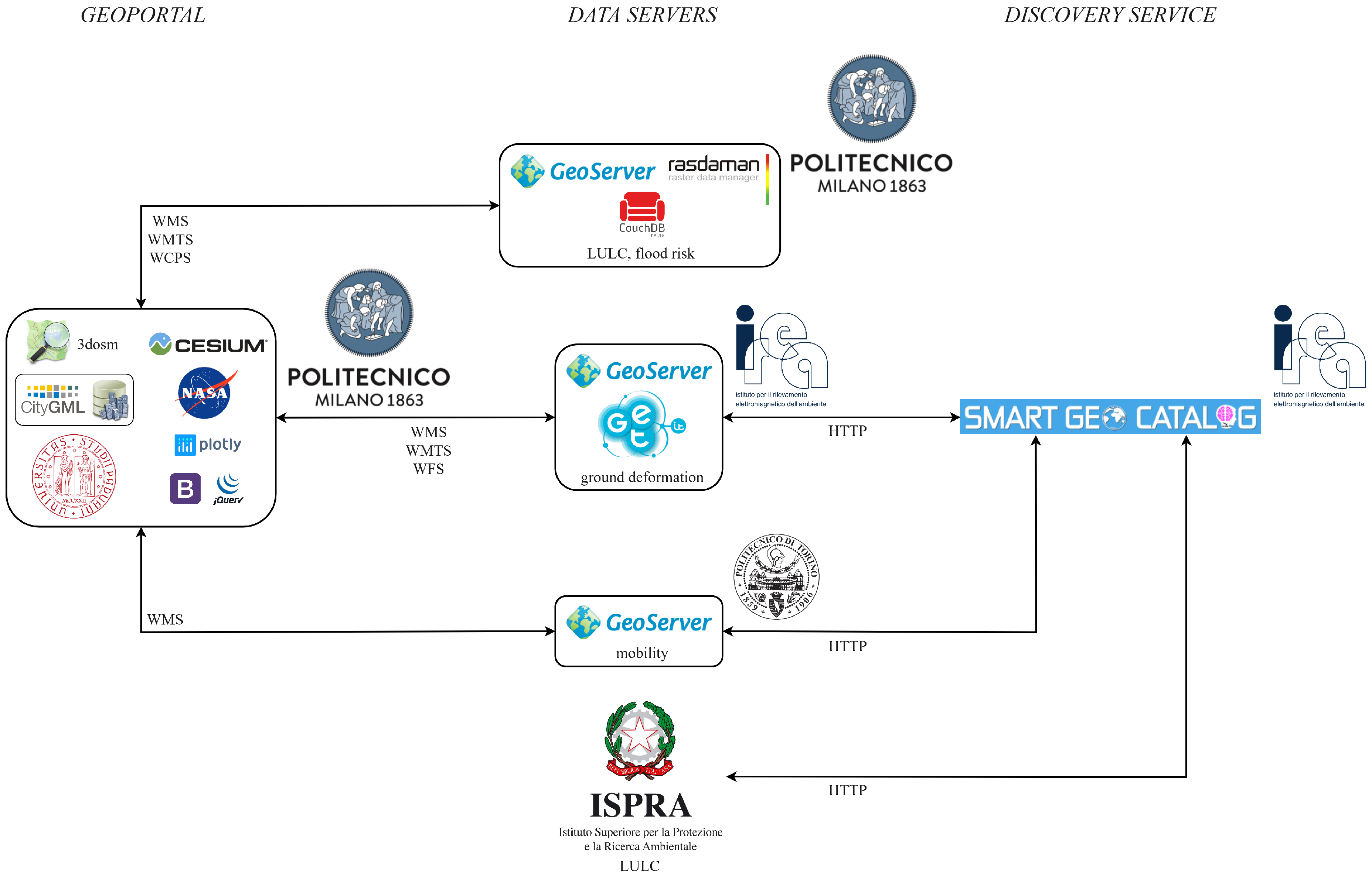
The open standards and FOSS that were used for tackling the challenges presented in the previous section through developing the geoportal of the URBAN GEO BIG DATA project are described in this section. The standards and software cover a wide range of functionalities, primarily storage, visualization, query and processing of big multidimensional geospatial data in vector or raster format. Their strategies for dealing with such data that were utilized include tiling and indexing to access data faster and parallel processing. The standards and software were chosen in a way to ensure interoperability of and cross-platform access to the geoportal. The overview of the project can be obtained from Figure 1.
2.1. Open Standards
The application programming interfaces (APIs) employed for geovisualization that are described in the Section 2.2 use Web Graphics Library (WebGL), a cross-platform and royalty-free web standard for a low-level graphics API, designed and maintained by the non-profit Khronos Group. The implementation of the standard is a JavaScript API for rendering interactive 2D and 3D graphics within a web browser without a plug-in as the API closely conforms to Open Graphics Library for Embedded Systems (OpenGL ES) that can be used in Hypertext Markup Language 5 (HTML5) canvas elements.
The geospatial data are retrieved by the client from several servers using the open web standards of Open Geospatial Consortium (OGC). The OGC standards deliver or process the raw geospatial data or deliver the portrayal of the raw geospatial data stored on a server or multiple servers. The OGC standards used are Web Map Service (WMS), Web Map Tile Service (WMTS), Web Feature Service (WFS), Web Coverage Service (WCS) and WCPS.
WMS produces maps of georeferenced data dynamically from geospatial data. A map is a portrayal of geospatial data as a digital image suitable for display on a computer screen, as a result, it is not the data. Styled Layer Descriptor (SLD) defines how a WMS can be extended to allow user-defined symbolization and colouring of geographic features and coverage data using Extensible Markup Language (XML) encoding. SLD is an OGC specification. WMTS provides a complementary approach to WMS. WMS generates a map dynamically, possibly using an SLD document for rendering with a custom style. WMTS trades the flexibility of custom map rendering for the scalability possible by serving predefined image tiles. Serving static data allows the implementation of a WMTS using a web server that simply returns existing files and the use of standard network mechanisms for scalability such as distributed cache systems. On the contrary, WFS offers access to geographic data at the feature and feature property level. It allows clients to retrieve, modify, replace and delete the data they are seeking, rather than a file that contains the data they are seeking.
The WCS has a mandatory Core, around which extensions can be implemented. WCS Core offers coverage access, subsetting and format encoding. Subsetting a coverage allows trimming and slicing. Trimming returns a coverage with the same number of dimensions as the input coverage. On the other hand, slicing returns a coverage with a reduced number of dimensions compared to the input coverage (see Figure 2).
The list of WCS Core extensions can be found in [33]. The one that is relevant to this is work is WCPS. WCPS defines a protocol-independent language for the extraction, processing and analysis of multidimensional coverages representing sensor, image or statistics data. It allows coverage analytics through appending a single parameter query to the WCS request, which contains a WCPS query string. Concisely, WCPS allows:
- Subsetting (downloading a subset of a coverage by trimming or slicing);
- Range subsetting (extracting a band or bands of a coverage);
- Condensing (consolidating cell values of a coverage along selected axes to a scalar value based on a condensing operation, such as calculating minimum, maximum, average or sum of the cell values);
- Constructing a coverage (creating a new coverage on the fly and filling it with values resulting from a processing expression evaluation);
- Applying induced operations (using a unary or binary function, that may include arithmetic, comparison, Boolean, trigonometric and logarithmic operations and case distinction that works on a single cell and applying it to all the cells of a coverage simultaneously).
As coverages are a superset of datacubes, the standards related to coverages are used to implement services for accessing and processing datacubes. Ref. [33] defined a datacube as:
A datacube is a massive multidimensional array, also called ’raster data’ or ’gridded data’; ’massive’ entails [...] sizes significantly beyond the main memory resources of the server hardware—otherwise, processing can be done satisfactorily with existing array tools like MATLAB or R.
The datacube concept heralds increased access to EO data, including additionally the time axis. Datacubes simplify access to multi-temporal geospatial data by constituting a 3D array (x/y/t) for raster time series. Moreover, datacubes may constitute 1D sensor time series, 2D imagery, 3D (x/y/z) subsurface voxel data, 4D (x/y/z/t) climate and ocean datacubes and even 5D atmospheric data with two time dimensions [33]. In this work, 2D imagery and 3D array (x/y/t) for raster time series were used. As a result, hereafter, whenever the term coverage is used in relation to the WCPS standard, the data are in raster format.
Moreover, in terms of open data standards, City Geography Markup Language (CityGML), JavaScript Object Notation (JSON), GeoJSON and Geographic Tagged Image File Format (GeoTIFF) were used. CityGML is an OGC encoding standard and represents an open data model and XML-based format for virtual 3D city models. Furthermore, GeoJSON is an open standard geospatial data format based on JSON.
2.2. Free and Open Source Software
There are various APIs for creating virtual globes on the web. Among them, the two most prominent ones are NASA Web WorldWind and CesiumJS. Both APIs offer high-performance, dynamic, interactive and cross-platform visualization and exploration of a virtual globe with terrain and 2D and 3D geospatial data layers on it. Both utilize WebGL, JavaScript, HTML5 and Cascading Style Sheets Level 3 (CSS3).
Today, many proprietary and open source tools support CityGML. An exhaustive list regarding these tools can be found in the wiki of CityGML (http://www.citygmlwiki.org/). The 3D City Database (3DCityDB) is one of these tools. It is a geodatabase for storing and managing virtual 3D city models on top of a standard spatial relational database (Oracle Spatial or Locator or PostgreSQL with PostGIS). The database schema fully implements the CityGML 1.0.0 and 2.0.0 standards. The database model contains semantically rich, hierarchically structured, multi-scale city objects facilitating complex GIS modelling and analysis tasks, beyond visualization. 3DCityDB Importer/Exporter is a Java-based application for importing data in CityGML format and exporting tiled data in Keyhole Markup Language (KML), Collaborative Design Activity (COLLADA), GL Transmission Format (glTF) or CityGML formats. 3DCityDB-Web-Map-Client extends CesiumJS for 3D visualization and interactive exploration of arbitrarily large semantic virtual 3D city models on the web. It allows visualizing large and tiled data in KML, COLLADA, glTF formats obtained using the 3DCityDB Importer/Exporter along with terrain and vector and raster layers.
GeoServer is a Java-based FOSS server for sharing geospatial data using open standards. It implements WMS, Transactional WFS and WCS. Additionally, WPS, WMTS and Catalogue Service for the web (CSW) implementations are provided as extensions. The clients that request the geospatial data published on GeoServer are typically web browsers and desktop GIS software. GeoServer has a management interface available on a web browser that connects to the data sources at the back-end. Moreover, GeoWebCache (GWC) is integrated into GeoServer. GWC is a Java-based free and open source web application for caching map tiles coming from various sources.
rasdaman (raster data manager) has been developed for more than two decades into a cross-domain datacube engine over a series of projects [34,35,36,37,38,39,40]. The raster query language of rasdaman, rasql extends Structured Query Language (SQL) with declarative nD array operators [41]. A separate layer adds geo semantics, such as information about regular and irregular grids and coordinate reference systems (CRSs), by implementing WMS 1.3, WCS 2.0 and WCPS 1.0. For OGC and INSPIRE WCS and OGC WCPS rasdaman is the reference implementation. rasdaman is the only available implementation for OGC WCPS.
3. Results
In the following sections, each application is explained in detail with the datasets they employed, their software development details and functionalities. When the background or literature diverges from the one given in the first two sections, they are given in a concise manner.
3.1. Multidimensional Vector Geospatial Data Visualization
3.1.1. OSM Data Visualization
OpenStreetMap (OSM) was founded in 2004 and has become a collaborative project that created a free and editable map of the world. OSM is one of the most prominent VGI projects. VGI, coined by [42], is a specific case of the more general phenomenon, user-generated content (UGC) from Web 2.0. VGI is geospatial UGC, i.e., geospatial data collected by individuals voluntarily [43]. OSM database contains crowdsourced geospatial data that are open, licensed under Open Database License (ODbL) [44].
Since 2008, people more and more often have collected data that can be used for creating 3D objects, such as height and roof geometry data [45]. Being able to constitute 3D objects from VGI sources is important, not only because we live in a 3D world, but also because 3D data allow the development and provision of many applications. The applications include providing a virtual 3D model of a city for demonstrating future city development plans to the public [46], visibility analysis [47], decision support for emergency [48,49,50], visualizing topological relations [51] and determining the environmental quality of public spaces [52]. Various applications use OSM data for building 3D objects. A comprehensive list is available in the wiki of OSM (https://wiki.openstreetmap.org/wiki/3D). Moreover, extensive research has been carried out related to this topic [45,53,54,55,56].
The 3D OSM Plugin API was developed for NASA Web WorldWind in the Google Summer of Code (GSoC) program in 2017. The source code of the API is available on GitHub (https://github.com/kilsedar/3dosm) with MIT License. The API provides a way to visualize OSM data in 2D and 3D on a virtual globe created using NASA Web WorldWind. Only buildings are visualized in 3D; the rest of the features are visualized in 2D. The spatial quality of OSM buildings was checked by comparing the OSM data of the Lombardy region of Italy whose capital is Milan with the region’s authoritative dataset. As a result, it was found that the positional accuracy of the OSM buildings is comparable with the quality of the authoritative dataset at scale 1:5000, as a result, they are suitable to use for the visualization developed in this work [57].
The 3D OSM Plugin API fetches the OSM data based on a tag and the bounding box of the area for which the user wants to retrieve elements. Overpass API was used for fetching the data. Overpass API is a read-only API that serves a selected part of the OSM database. A client sends a query to the API and gets the data that correspond to the query. It has two query languages: Overpass XML and Overpass Query Language (Overpass QL). The Overpass QL was used to construct the queries. Overpass API returns the data in JSON format. The data in JSON format were converted to GeoJSON format using the osmtogeojson API (https://github.com/tyrasd/osmtogeojson). Besides getting data using the Overpass API, it is possible to use a file in GeoJSON format or write the data in GeoJSON format inside JavaScript code. Only the GeoJSON data obtained in the way that the 3D OSM Plugin API does were tested and the results were as expected.
The height of the buildings that are visualized in 3D can be set using the OSM database, more specifically, the tags of features. First, the height key (https://wiki.openstreetmap.org/wiki/Key:height) that describes the height of a feature is used to set the height of a building, if a value is assigned to it for an element with the building key (https://wiki.openstreetmap.org/wiki/Key:building). If a value for such a height key is not defined, the building:levels key (https://wiki.openstreetmap.org/wiki/Key:building:levels) that describes the number of above-ground levels of a building or part of a building is used to set the height of a building, if a value is assigned to it. Each level is assumed to be 3 m. If a value is not assigned to either key, the building is assumed to have five levels, i.e., be 15 m long. A comprehensive list of OSM keys that can be used to render 3D buildings is available in the wiki of OSM (https://wiki.openstreetmap.org/wiki/Simple_3D_buildings). As these tags are not present most of the time, the API lets the user use a file in GeoJSON format obtained in the way described above, with an additional attribute that denotes the building heights. According to the publication [45], less than 1.5% of the elements with building key in the OSM database had the height key in November 2011. Moreover, it is possible to set an arbitrary value for all the buildings. It is also possible to visualize the buildings in 2D.
The style of the OSM elements can be set using the API that employs two classes of NASA Web WorldWind: PlacemarkAttributes and ShapeAttributes. PlacemarkAttributes class is used for Point and MultiPoint Geometry types of GeoJSON. ShapeAttributes class is used for the rest of the Geometry types of GeoJSON and triangle meshes. Using the PlacemarkAttributes class, it is possible to set the image and label of placemarks, among others. Using the ShapeAttributes class, it is possible to set the interior and outline colour, outline width, whether to draw an outline, among others. The user can choose to set varying colours for the 3D visualization of buildings. The colours depend on the height of the buildings in the dataset and the colour and thresholds defined by the user. As the height of the buildings increases, the red component in the colour in RGB gets a higher value. Moreover, the thresholds that are ordered hold the values for building heights, and single colour is assigned to all the buildings with a height between two consecutive thresholds. In this way, a 3D heatmap that represents building heights is generated.
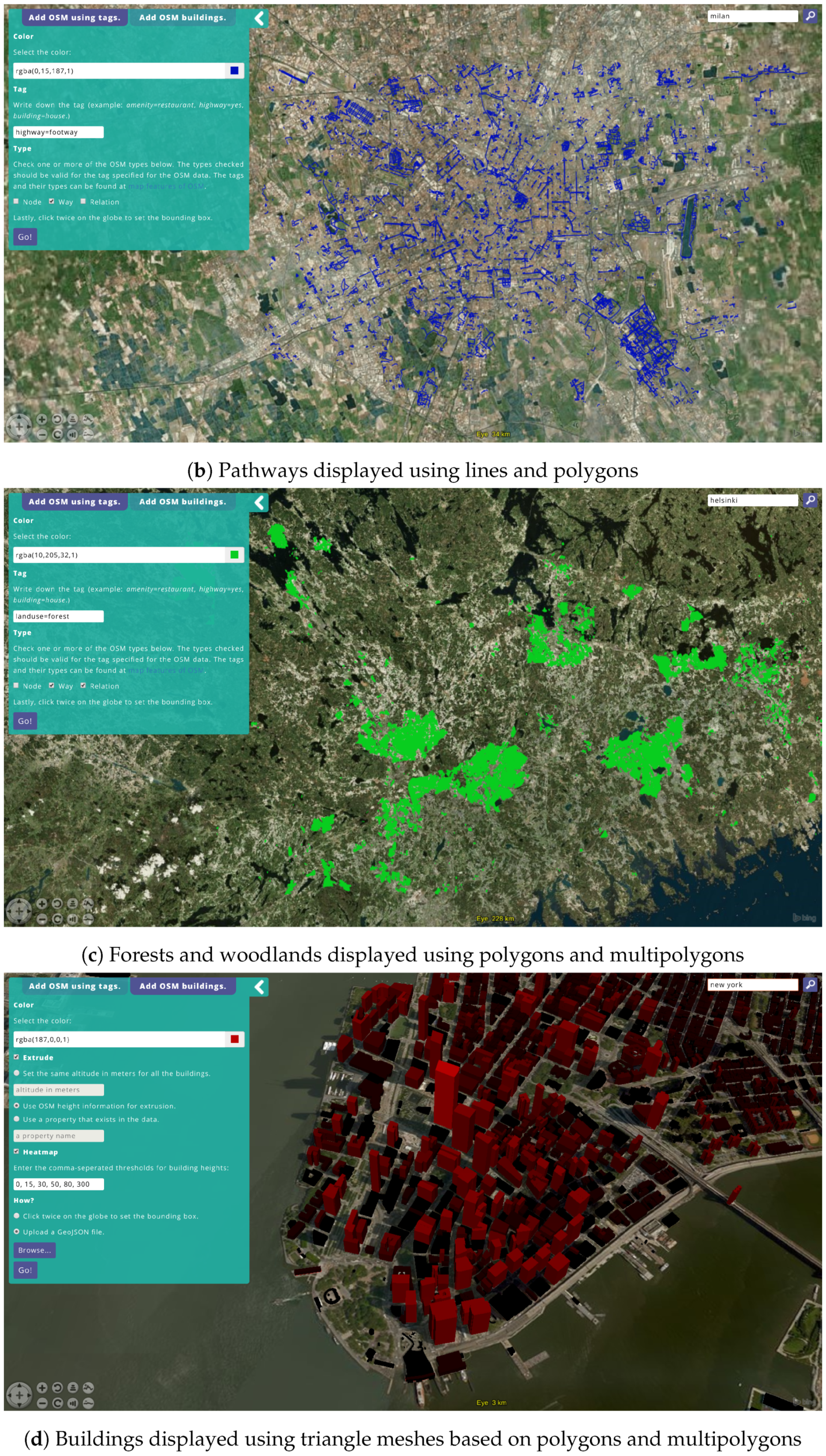
The authors participated in NASA Europa Challenge 2017 with an application that uses the 3D OSM Plugin API. Figure 3 displays screenshots from the application and exemplifies the capabilities of the API. The elements that are in the bounding box drawn on the virtual globe by the user can be retrieved from the OSM database. Moreover, the tag and colour of the elements can be defined by the user using the graphical user interface (GUI) of the application. Figure 3a shows the amenities in Istanbul displayed using placemarks. The nodes were retrieved from the OSM database using the amenity=yes tag (https://wiki.openstreetmap.org/wiki/Key:amenity). Figure 3b shows the pathways that are used exclusively or mainly by pedestrians in Milan displayed using lines and polygons. The ways were retrieved from the OSM database using the highway=footway tag (https://wiki.openstreetmap.org/wiki/Tag:highway=footway). Figure 3c shows the forests and woodlands in Helsinki displayed using polygons and multipolygons. The ways and relations were retrieved from the OSM database using the landuse=forest tag (https://wiki.openstreetmap.org/wiki/Tag:landuse=forest).
Figure 3d shows the buildings in New York displayed using triangle meshes based on polygons and multipolygons. The ways and relations were retrieved from the OSM database using the building=yes tag. This visualization uses the values of the keys height and building: levels associated with the elements that represent a building to set the height of the triangle meshes. This visualization clearly shows the varying height of the buildings, which is because for most of the elements that represent a building in New York the height or building:levels keys with an assigned value exist.
However, as most of the elements that have the building key do not have the height or building:levels key, when possible, an alternative way was used to set the building heights. First, LIDAR data that represent digital terrain model (DTM) and digital surface model (DSM) were used to extract the height of the buildings in Milan. LIDAR data were received from the Ministry for Environment, Land and Sea Protection of Italy using the contact information available at the national geoportal (http://www.pcn.minambiente.it/mattm/en/data-distribution-service-pst/). Then, they were converted to virtual datasets (VRTs) using the gdalbuildvrt program of Geospatial Data Abstraction Library (GDAL). Then, the VRTs of DTM and DSM were imported into GRASS GIS. The procedure involves subtracting DTM from DSM to get the height of the objects on the terrain using the r.mapcalc module of GRASS GIS. The OSM data that contain the building footprints in Milan were downloaded in GeoJSON format using Mapzen Metro Extracts and imported into GRASS GIS. Using the v.rast.stats module of GRASS GIS, some statistics were calculated for the footprints of the buildings. The calculated statistics were the minimum, maximum, average and median of the values of pixels inside each footprint. Among these statistics, the median was used to discard the outliers that may stem from the misalignment between the footprints in the OSM data and LIDAR measurements. Second, Urban Atlas Building Height 2012 dataset in GeoTIFF format provided by the Copernicus Programme (https://land.copernicus.eu/local/urban-atlas/building-height-2012) was used to extract the height of the buildings in Rome. The only difference between this procedure and the previous one is the removal of subtraction between DTM and DSM, as the raster data already represent the building heights. For the other three cities the URBAN GEO BIG DATA project focuses on (i.e., Padua, Turin and Naples), the height and building:levels keys associated with the elements that represent a building were used to set the building heights.
3.1.2. CityGML Data Visualization
Besides VGI (i.e., OSM data in GeoJSON format), 3D vector data visualization was achieved using the OGC standard for representing 3D vector data that pertain to urban areas, CityGML. The visualization of the data in CityGML format would ideally be achieved using the 3D Tiles standard, as it is designed for streaming and rendering massive 3D geospatial data and using an OGC standard is consistent with the goal of achieving interoperability. Moreover, CesiumJS supports the 3D Tiles format. It is important to note that there are other OGC standards for 3D geospatial data delivery, such as 3D Portrayal Service (3DPS) and Indexed 3D Scene Layers (I3S), yet they are not supported by CesiumJS. However, there is not FOSS for converting data in CityGML format to 3D Tiles format. As a result, 3DCityDB was used for the visualization of the data in CityGML format in the URBAN GEO BIG DATA project.
Virtual 3D city models in CityGML format have been created for many cities in the world, yet they are not available for the five cities that the URBAN GEO BIG DATA project focuses on. For this reason, the team from the University of Padua developed software called shp2city that converts data in Esri shapefile format to CityGML format [58]. In the URBAN GEO BIG DATA project, CityGML datasets that represent the buildings of Milan, Padua, Turin and Naples were generated using the shp2city software. Using 3DCityDB Importer/Exporter, the datasets were imported into a PostgreSQL database extended with PostGIS. Then, using the same software they were exported in KML, COLLADA, glTF formats tiled. The exported datasets were visualized using the 3DCityDB-Web-Map-Client. Since the buildings in the CityGML datasets have altitude values, it is possible to place them on the terrain. On the geoportal, it is also possible to simulate the sun, which enables to visualize shadows of the terrain and buildings at different times of the day and year. Moreover, six base maps were provided in the geoportal when CesiumJS was used to create the virtual globe, which are Bing Maps Aerial, Mapbox Satellite Streets, OSM, CARTO Dark, Stamen Terrain and Stamen Watercolor. The geoportal enables to switch between these six base maps.
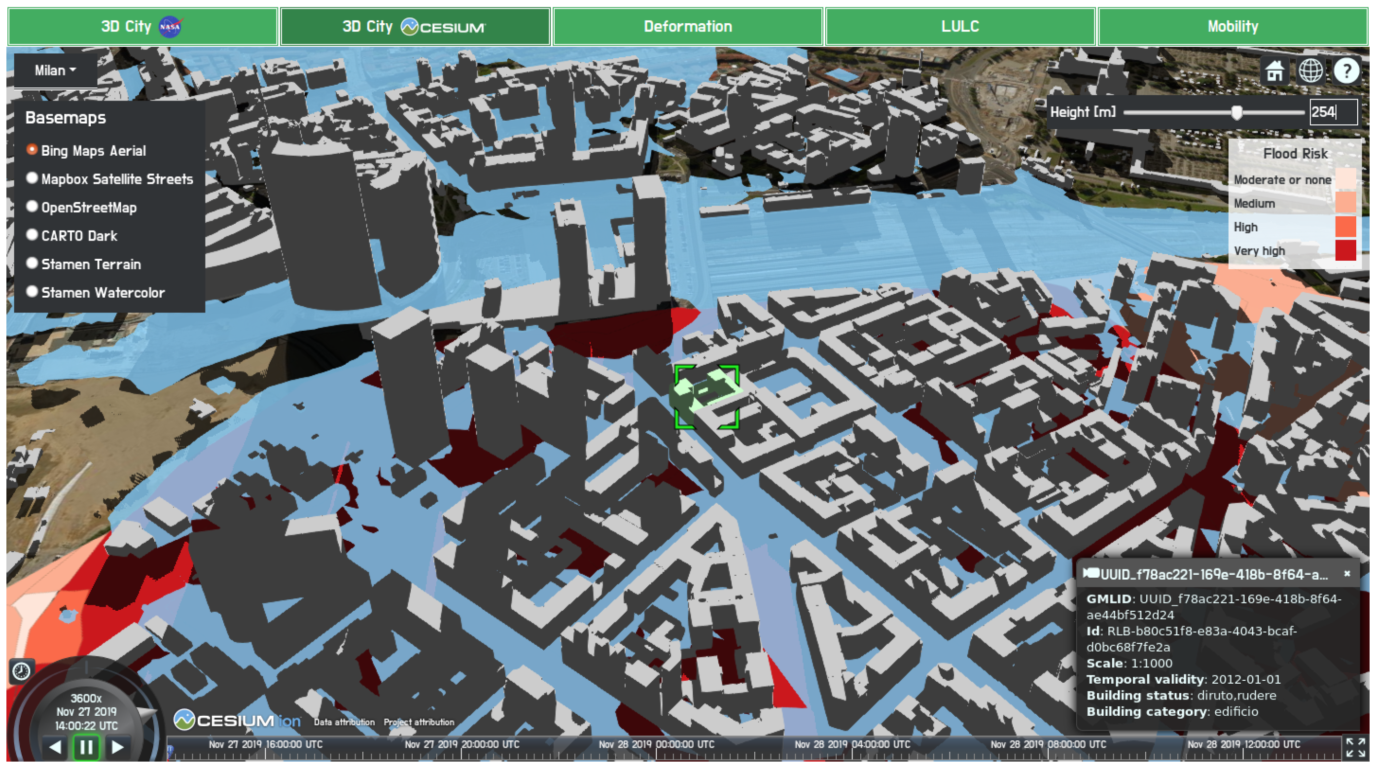
Virtual 3D city models in CityGML format have been used for various applications, such as noise propagation simulation and mapping, energy-related assessments of buildings, indoor navigation, disaster management and homeland security [59,60]. Disaster management applications include flood simulations for assessing the flood risk and potential damage at a micro-scale [61,62,63,64,65]. In this work, virtual 3D city models in CityGML format were used for flood simulation. A semi-transparent polygon was placed on the ellipsoid surface of the virtual globe that users can extrude in meters using a slider in the GUI of the geoportal. It is possible to use the VRTheWorldTerrainProvider class of CesiumJS to generate the terrain geometry by tessellating the digital elevation model (DEM) that includes both land topography and bathymetry with a 90-m resolution for the entire globe provided by the VR-TheWorld Server (https://www.mak.com/products/terrain/vr-theworld-server). Instead of using the DEM provided by the VR-TheWorld Server, a 5-m DTM of Milan in GeoTIFF format was used to construct the terrain of the virtual globe to increase the accuracy of the flood simulation. This dataset is published by the Lombardy region (http://www.geoportale.regione.lombardia.it/en/home) as open data. The first step for using the DTM of Milan to construct the terrain of the virtual globe was creating terrain tiles in quantized-mesh-1.0 format (https://github.com/AnalyticalGraphicsInc/quantized-mesh). The tiles were created using the Cesium Terrain Builder (https://github.com/ahuarte47/cesium-terrain-builder). Then, the Cesium Terrain Server (https://github.com/geo-data/cesium-terrain-server) was used to host the tiles. The geoportal refers to this server to retrieve the tiles. Following this approach, it is not possible to simulate floods anywhere else in the world as the DTM is only for Milan unless additional local DEM or DTM is used to construct the terrain of the virtual globe. Finally, the flood risk map of Milan published by the Lombardy region as open data was stored on GeoServer and tiled using GWC. The ImageryLayer and WebMapTileServiceImageryProvider classes of CesiumJS were used by the client to make requests to the WMTS implementation of GeoServer and place the retrieved tiled imagery on the virtual globe. More information was given by [66]. Figure 4 summarizes the software used and their interactions to clarify the content given above. Figure 5 displays a flood simulation in Milan with the flood risk map and the visualization of the CityGML data that represent buildings.
3.2. Multidimensional Raster Geospatial Data Visualization, Query and Processing
3.2.1. Ground Deformation Visualization and Query
Differential Synthetic Aperture Radar Interferometry (DInSAR) is a well-established technique for the mapping and continuous monitoring of the areas on Earth that are subject to ground deformation [67]. National Research Council of Italy (CNR) Institute for Electromagnetic Sensing of the Environment (IREA) used the Small BAseline Subset (SBAS) technique, which is a DInSAR algorithm [68], to generate the mean deformation velocity maps and deformation time series for Milan, Padua, Turin, Naples and Rome. The deformation data give information on the changes of the Earth’s surface with a direction and magnitude in a metric unit, which enables monitoring natural hazards and environmental alterations due to subsidence and agriculture, among others. This information facilitates determining the parts of the monitored areas that are susceptible to damage in case of natural hazards and the structures that are susceptible to damage or collapse as a result of or independent from natural hazards.
The SBAS algorithm was applied to the sequences of archived synthetic aperture radar (SAR) images collected by the European Remote Sensing (ERS) and Environmental Satellite (Envisat) satellites of ESA from 1992 to 2010. A maximum perpendicular baseline of 400 m and a maximum period of two years were used for the selection of the small baseline interferometric data pairs for the areas of interest in the five cities. Deformation data were produced at medium spatial resolution and for some parts of the residential and central regions of the areas of interest also at full spatial resolution.
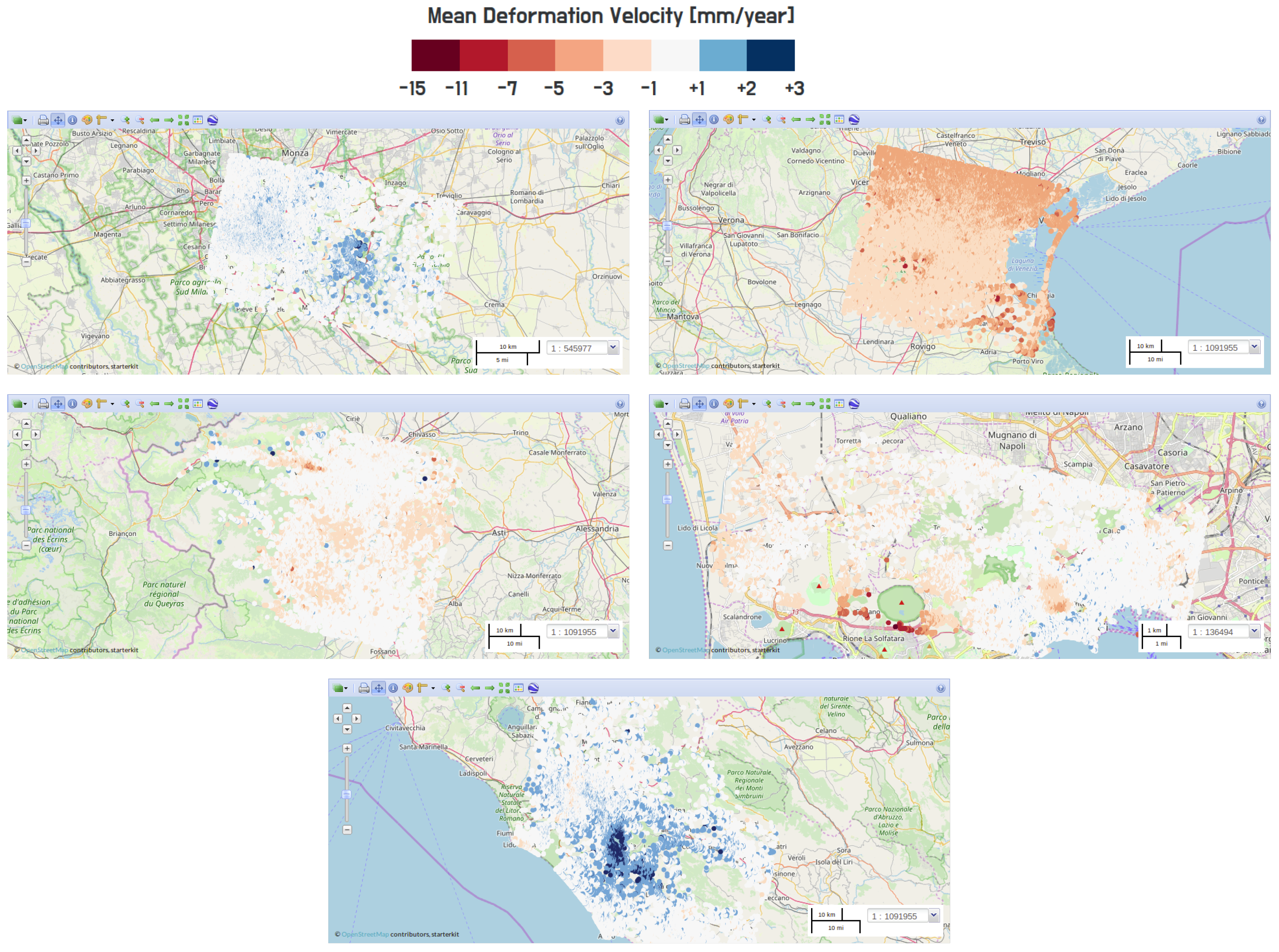
The mean deformation velocity maps and deformation time series of the five cities are available on a Geoinformation Enabling ToolkIT starterkit® (GET-IT) (http://www.get-it.it/) installation (https://ugbd.get-it.it/). GET-IT is developed at CNR IREA within the flagship project RITMARE (http://www.ritmare.it/en/) starting from a widely known geospatial content management system (CMS) GeoNode [69]. GET-IT can be used to visualize and download geospatial data. Moreover, it can be used to read and download the metadata of the geospatial data. The visualization of the mean deformation velocity maps for the five cities is given in Figure 6.
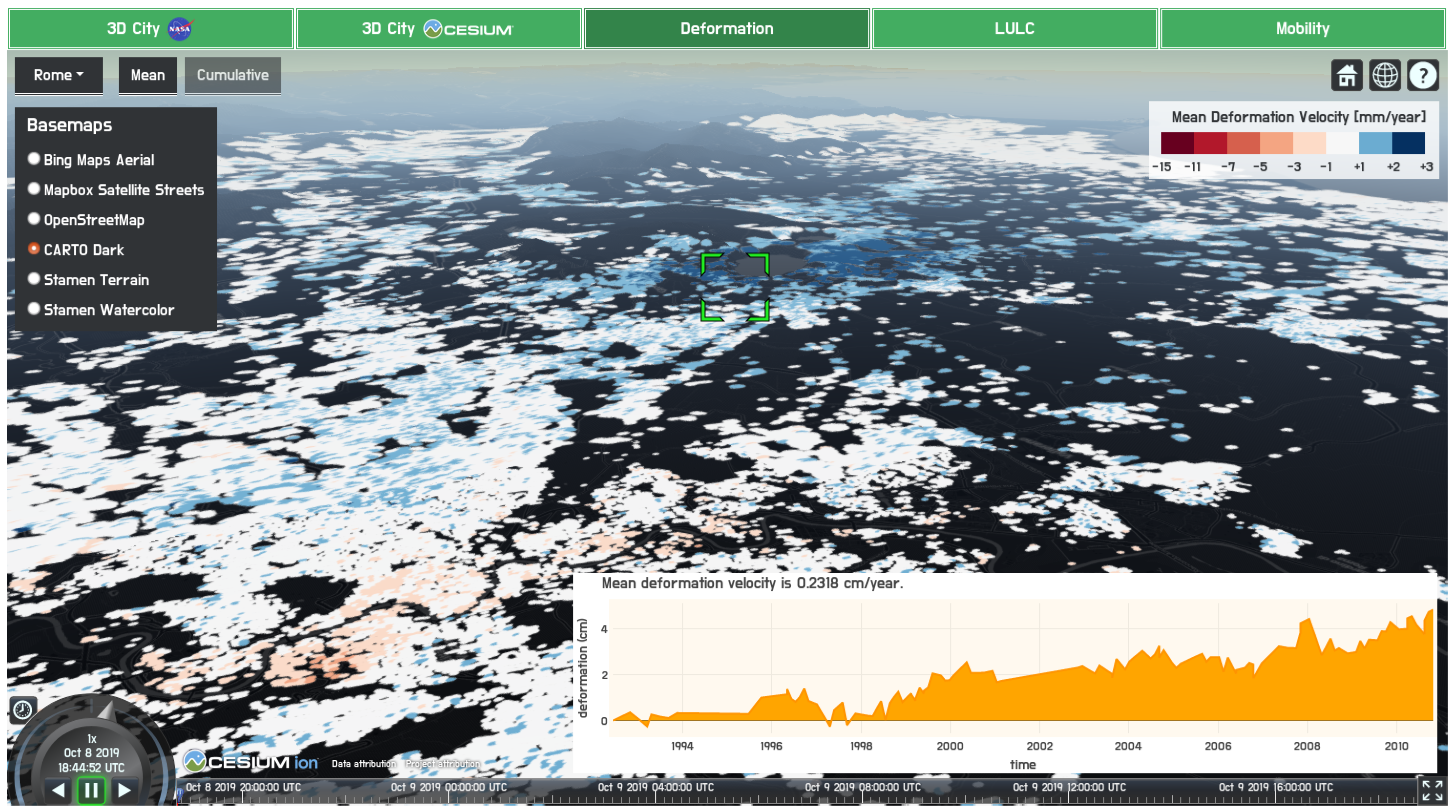
A mean deformation velocity map was retrieved by making a request to the GET-IT instance of the URBAN GEO BIG DATA project, using the WMS implementation of GeoServer. The ImageryLayer and WebMapServiceImageryProvider classes of CesiumJS were used by the client to make the request and place the retrieved image on the virtual globe. Each deformation point can be clicked on to display its cumulative deformation time series using a plot created employing a JavaScript API Plotly (https://github.com/plotly/plotly.js). The data used to create the plot were retrieved in JSON format by making a request to the GET-IT instance of the URBAN GEO BIG DATA project, using the WFS implementation of GeoServer. The style of the maps was defined using SLD encoding in GeoServer. The colour scheme for mean deformation velocity used in the URBAN GEO BIG DATA project is given in Figure 6. The visualization of the mean deformation velocity map of Rome and the plot of cumulative deformation time series of a deformation point is displayed in Figure 7. Plotting cumulative deformation time series is available for all the deformation points of the five cities.
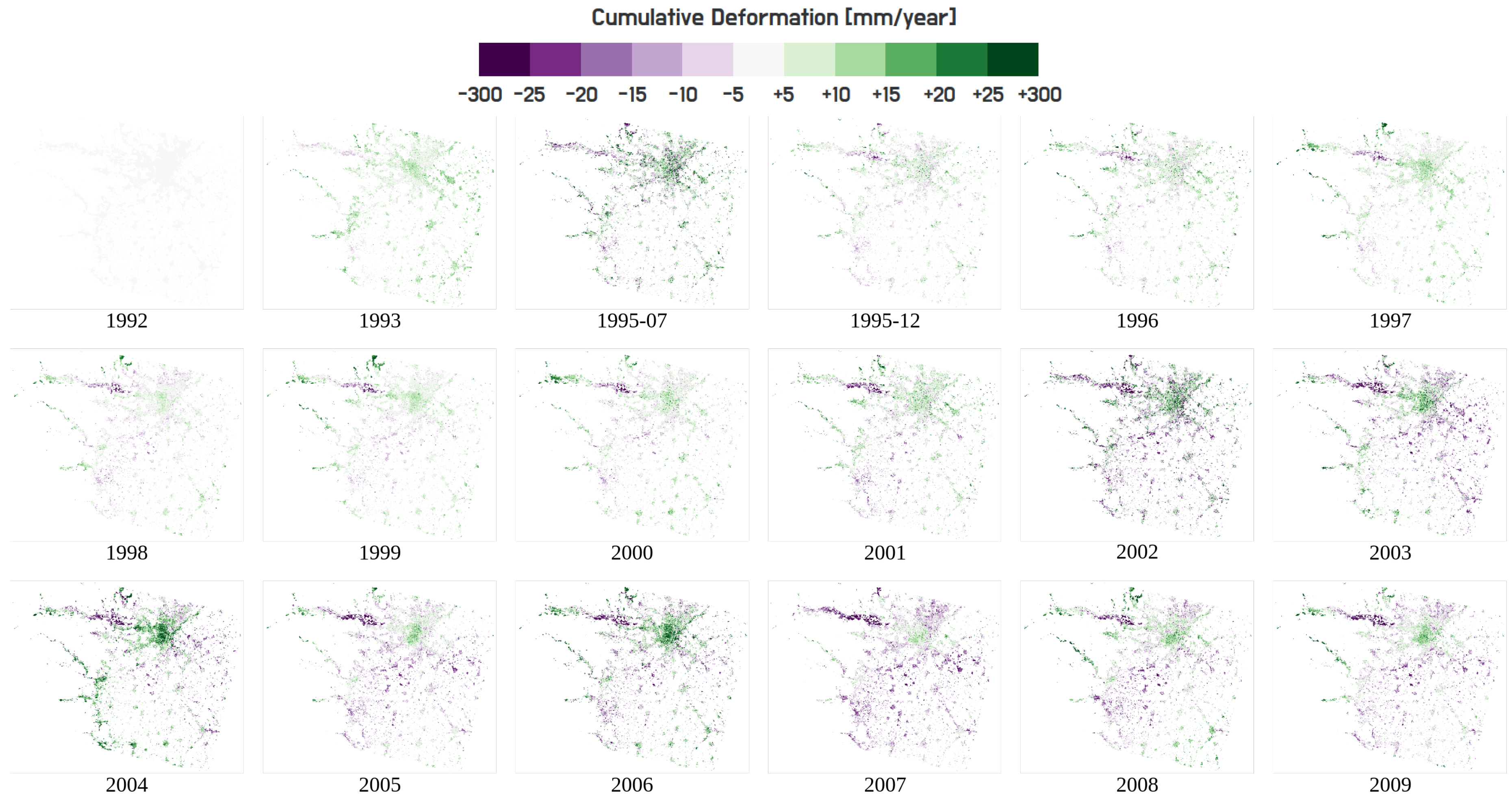
Furthermore, raster files that represent cumulative deformation were generated for almost every year and the five cities, so that an overview of deformation for eighteen years can be achieved by temporally animating raster images. The raster files in GeoTIFF format were derived from the deformation time series. Ref. [70] explained the method for creating the raster files, which have reduced spatial and temporal resolution; as a result, the deformation time series were summarized. The ImageMosaic data store of GeoServer was used for creating raster time series. An ImageMosaic was created for each of the five cities. The colour scheme for cumulative deformation used in the URBAN GEO BIG DATA project and the visualization of the raster deformation time series of Turin are given in Figure 8. The figures show the decreasing, increasing and periodic changes of deformation.
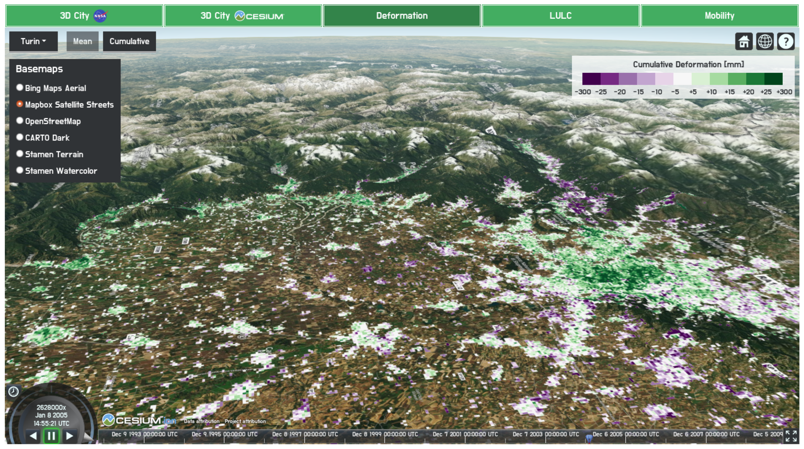
An animation is available for each ImageMosaic. An ImageMosaic was temporally animated employing the animation and timeline widgets of CesiumJS created using the library’s Animation and Timeline classes. The raster time series in ImageMosaic format comprises of multiple raster files, each having a timestamp. Thus, an animation is available for each ImageMosaic created in this work where each frame of the animation corresponds to a raster image with a timestamp. The animation can be initiated, paused and played forward and reverse using the animation widget. Moreover, using the timeline widget, it is possible to scroll through time manually. Animation and timeline widgets and the visualization of the raster file of 2005 from the raster deformation time series of Turin can be seen in Figure 9. The geoportal allows zooming to each of the five cities using a drop-down list. Once a city is selected using the list, either the mean deformation velocity map or the raster deformation time series of the selected city can be added to the virtual globe.
As the deformation data have both negative and positive values, the colour schemes adhere to the diverging schemes where equal emphasis is put on the mid-range and extremes at both ends of the data range. In diverging schemes, the break in the middle is emphasized with light colours, and the low and high extremes are emphasized with dark colours that have contrasting hues [71]. Diverging schemes with eleven classes were chosen using ColorBrewer 2.0 (http://colorbrewer2.org) [72]. The mid-range value was replaced with 0 in the colour schemes to define different colours for negative and positive values. Moreover, the intervals for colours in the colour scheme for mean deformation velocity do not exceed the standard deviation of about 1 mm/year for mean deformation velocity. Likewise, the intervals for colours in the colour scheme for cumulative deformation do not exceed the standard deviation of about 5 mm for deformation [73]. Considering the standard deviation and the diverging nature of the data, the colour schemes given in Figure 6 and Figure 8 were used. Both colour schemes were used for all the five cities to enable visual comparison among them. As the values for both mean deformation velocity and cumulative deformation concentrate around zero, the intervals become wider towards the low and high extremes.
3.2.2. LULC Visualization, Query and Processing
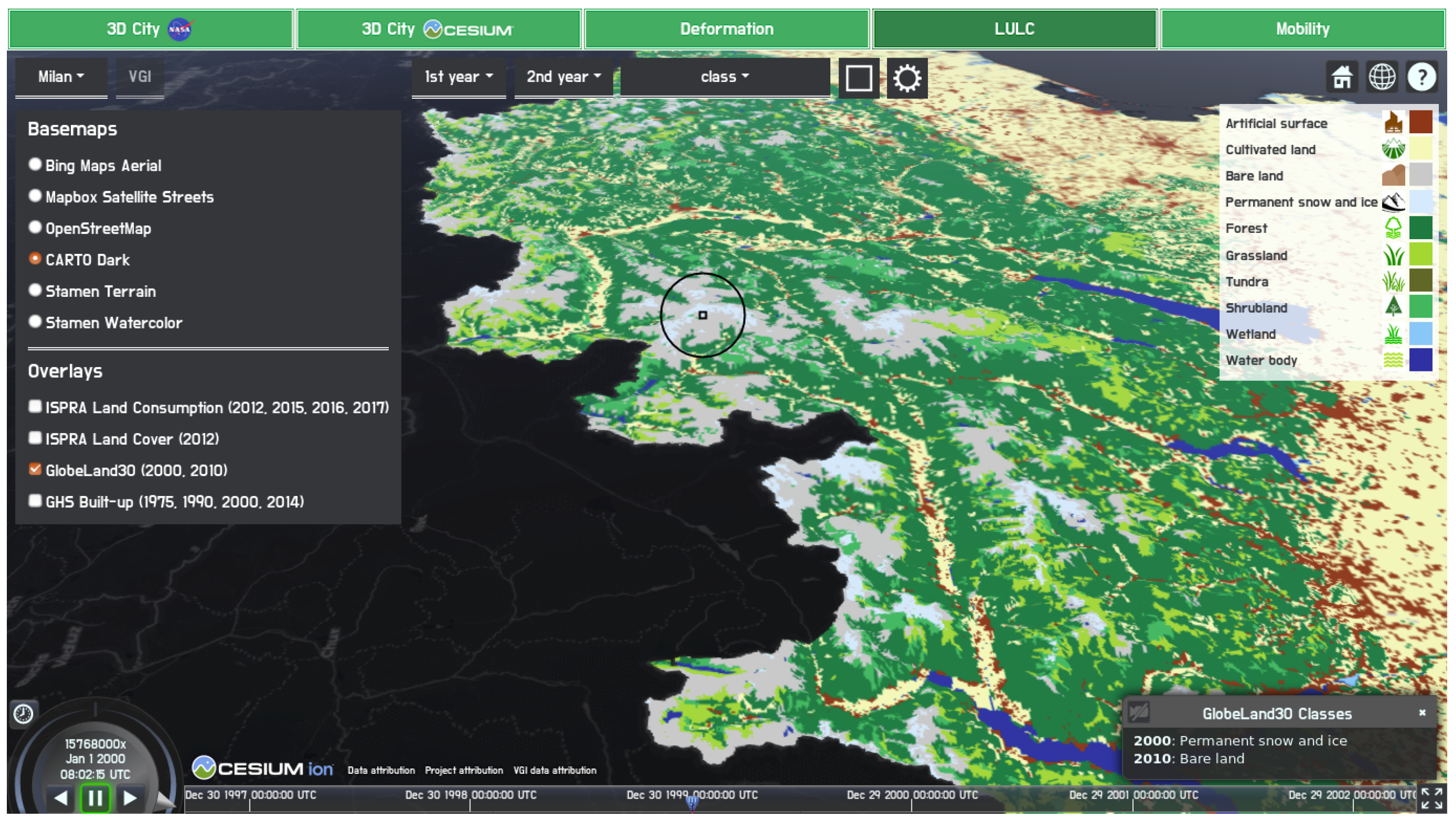
The growth of cities and as a result the increase of soil consumption [74] results in the decrease of life quality in the cities. One way it does so is by increasing the air temperature [75] which exacerbates health problems, especially for elders, during summertime. As a result, this work also focused on land use and land cover (LULC). EO-derived LULC datasets were visualized on a virtual globe on the web. Moreover, query and processing of the datasets can be initiated using the geoportal. The LULC datasets comprise of land consumption maps from the Italian Institute for Environmental Protection and Research (ISPRA) of 2012, 2015, 2016 and 2017 with 10-m resolution; land cover map from ISPRA of 2012 with 10-m resolution; GlobeLand30 of 2000 and 2010 with 30-m resolution and GHS built-up (GHS-BUILT) of 1975, 1990, 2000 and 2014 with 38-m resolution. GlobeLand30 and GHS-BUILT that are available globally were cropped to the boundary of Italy. The size of the land consumption maps from ISPRA is around 224 GB, the size of the land cover map from ISPRA is around 28 GB, the size of GlobeLand30 is around 2.94 GB and the size of GHS-BUILT is around 6.23 GB. The land consumption maps from ISPRA are considered to be land use maps, and the rest are considered to be land cover maps. The land consumption maps from ISPRA and GHS-BUILT have two classes that indicate if the area is consumed or not and is built-up or not, respectively. The land cover map from ISPRA and GlobeLand30 have more than two classes.
The style of all the LULC datasets was defined using SLD encoding in GeoServer. The geoportal allows zooming to each of the five cities using a drop-down list. The land cover map from ISPRA of 2012 was stored using the GeoTIFF data store, instead of the ImageMosaic data store of GeoServer as it is available for a single year. After publishing the dataset on GeoServer, it was tiled using GWC. The ImageryLayer and WebMapTileServiceImageryProvider classes of CesiumJS were used by the client to make requests to the WMTS implementation of GeoServer and place the retrieved tiled imagery on the virtual globe.
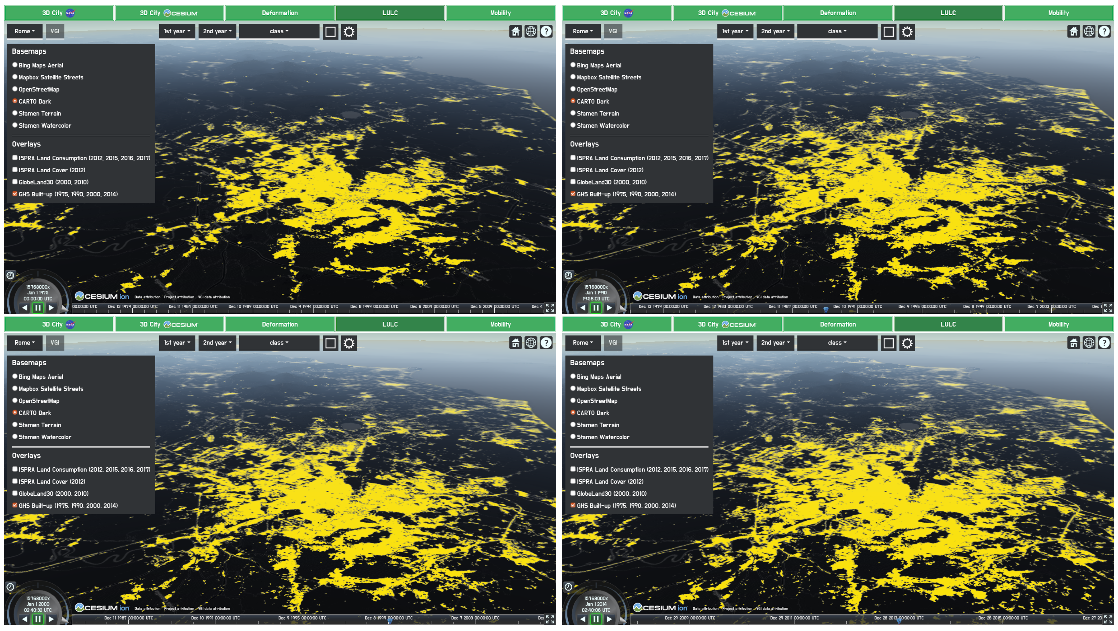
As already mentioned in the previous section, the ImageMosaic data store of GeoServer was used for creating raster time series. An ImageMosaic was created for the land consumption maps from ISPRA, GlobeLand30 and GHS-BUILT. An animation is available for each ImageMosaic, which was created using the method described in the previous section. GlobeLand30 and GHS-BUILT that are available globally were cropped to the boundary of Italy as the URBAN GEO BIG DATA project focuses on Italy and the limited storage capacity. Figure 10 shows that animation allows detecting the changes of land cover over time visually as it is visible that built-up areas increased steadily in Rome from 1975 to 2014 according to GHS-BUILT.
Furthermore, all the LULC datasets were imported into rasdaman so that they can be processed using WCPS. The datasets were imported using the web Coverage Service Transaction (WCS-T) implementation of rasdaman. As a result of the import of the sets of the datasets, a datacube was created that corresponds to each set of the datasets. Consequently, four datacubes were created. The datacube of the land cover map from ISPRA is 2D (x/y), while the rest of the datacubes are 3D (x/y/t).
Processing can be executed for both a set of coordinates and four sets of coordinates, i.e., a rectangle. When a user clicks on a pixel, the pixel coordinates of the canvas are translated into a set of coordinates in EPSG:3857 using CesiumJS. The processing, which represents a slicing operation, uses the set of coordinates and executes differently depending on the number of dimensions of the datacube. If the datacube is 2D, which is true for the land cover map from ISPRA, the processing returns the value of the pixel that is the land cover class. On the other hand, if the datacube is 3D, which is true for the land consumption maps from ISPRA, GlobeLand30 and GHS-BUILT, the processing returns the value of the pixel for all the times that the datasets are available, which corresponds to the land use or land cover classes. As a result, it is possible to get the change of land use or land cover classes over time for a pixel (see Figure 11).
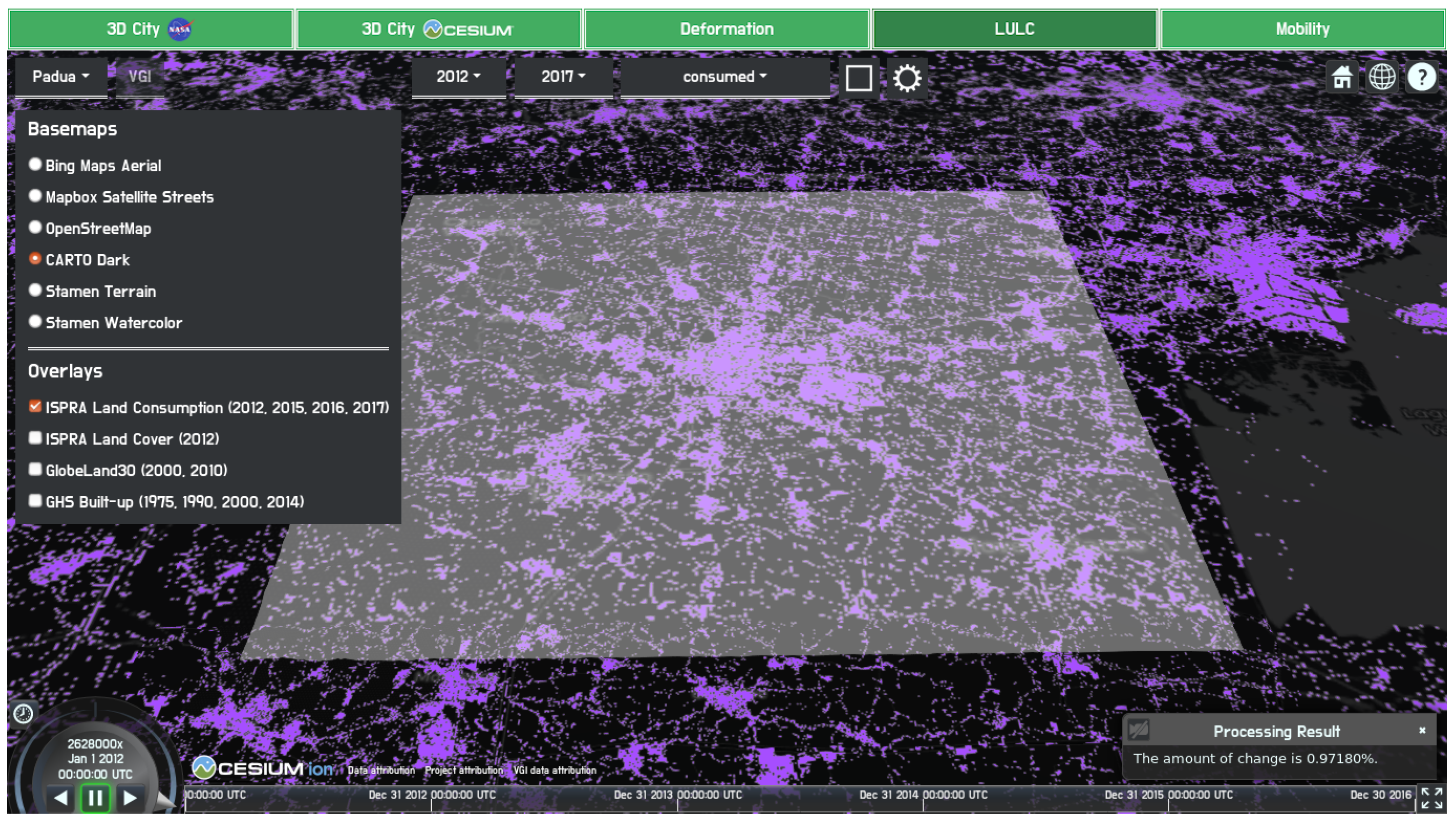
As mentioned earlier, the processing can also be executed for four sets of coordinates, besides a set of coordinates. The geoportal provides an interface for calculating the amount of change of a selected land use or land cover class inside a rectangle drawn by the user between two selected years. This operation is available only for 3D datacubes. The processing represents a combination of slicing and condensing operations. The four sets of pixel coordinates of the canvas that define the vertices of the rectangle are translated into four sets of coordinates in EPSG:3857 using CesiumJS.
The URLs executed (i.e., the requests made to the WCPS implementation of rasdaman) are http://urbangeobigdata.como.polimi.it:8081/rasdaman/ows?query=for$cin(ispra_lc_2012_2015_2016_2017)returnencode(count($c[X(xMin:xMax),Y(yMin:yMax),ansi(firstYear)]=classificationCode),“text/csv”) and http://urbangeobigdata.como.polimi.it:8081/rasdaman/ows?query=for$cin(ispra_lc_2012_2015_2016_2017)returnencode(count($c[X(xMin:xMax),Y(yMin:yMax),ansi(secondYear)]=classificationCode),“text/csv”) for processing the datacube of the land consumption maps from ISPRA for four sets of coordinates. The xMin variable stands for minimum longitude, xMax variable stands for maximum longitude, yMin variable stands for minimum latitude and yMax variable stands for maximum latitude. These variables have the values of the four sets of coordinates in EPSG:3857 that correspond to the vertices of the rectangle. The value of the firstYear variable is the first year and the value of the secondYear variable is the second year the user chooses using the drop-down lists in the GUI. The classificationCode variable has the value of the pixel in the raster file that corresponds to the class the user chooses using the drop-down list in the GUI. The query parameter’s value is a rasql query. For the other two datacubes, only the coverage id (i.e., ispra_lc_2012_2015_2016_2017) is different in the URLs. The requests calculate the number of pixels inside the rectangle drawn by the user that has the value of the classificationCode for the values of both the firstYear and secondYear. After getting the counts for both years, the percentage change is calculated and given to the user in a window created using the InfoBox class of CesiumJS (see Figure 12).
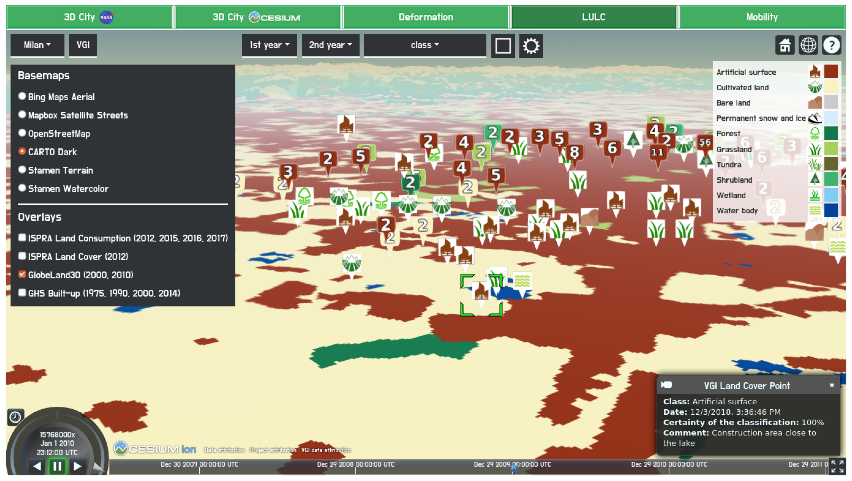
VGI was visualized on the LULC raster imagery on the virtual globe. There are plenty of other applications for the visualization of VGI on a 2D or 3D map [76,77,78]. In this work, the VGI is collected by an application called Land Cover Collector that enables the collection of land cover data according to GlobeLand30 nomenclature.
The VGI is retrieved from a CouchDB database in JSON format. Each object in the JSON data that corresponds to a single submission of VGI is represented by an object created using the Entity class of CesiumJS. The position of an Entity is determined by the values of the longitude and latitude properties of the JSON object that it corresponds to. For each Entity, BillboardGraphics class of CesiumJS was used to create a pin located at the position of the Entity. The icons of GlobeLand30 were adopted for creating the pins. When a user clicks on a pin, the values of the significant properties of the JSON object that corresponds to the clicked pin are displayed in a window created using the InfoBox class of CesiumJS. The significant properties are the land cover class, the date the land cover data were submitted, the certainty of the user regarding the land cover class they stated and if available the comment of the user.
All the JSON objects that have the same land cover class are represented by an object created using the CustomDataSource class of CesiumJS so that they can be clustered. Clustering enables to get a less cluttered visualization, which enables to get insights regarding the distribution of land cover classes on the virtual globe for each zoom level. Each cluster is displayed with a pin created using the PinBuilder class of CesiumJS. The pin of each cluster of a land cover class has the colour of the pixels in the raster imagery that represents the clustered land cover class. Moreover, the number of Entities in each cluster is displayed on the pin. The clusters that are represented by pins on the virtual globe are displayed in Figure 13. Besides, this visualization enables to identify the differences between the VGI collected according to GlobeLand30 nomenclature and GlobeLand30 raster imagery visually. The differences suggest errors in GlobeLand30, which call upon further investigation. The data collected using the Land Cover Collector application can be used as reference data to perform the validation of GlobeLand30 computationally [79,80,81].
3.2.3. Mobility Visualization
Datasets of public transportation networks and traffic (i.e., number of vehicles) for each of 24 h of a day (10 October 2018) were generated by the team from Politecnico di Torino and stored on a GeoServer installation. They were retrieved using the WMS implementation of GeoServer and the ImageryLayer and WebMapServiceImageryProvider classes of CesiumJS were used to make the requests and place the retrieved images on the virtual globe. As traffic datasets are available for multiple time ranges, they can be visualized using the animation and timeline widgets of CesiumJS, using the method used in the applications related to ground deformation and LULC. However, it is worth to note that, in this application instead of ImageMosaic data store of GeoServer, 24 datasets for each city stored in vector format on GeoServer were used. In Figure 14, the visualization of traffic in Rome between 12:00 and 13:00 UTC is given.
4. Conclusions
Cartography has traditionally produced 2D maps. Globes, even though they provide the advantage of undistorted representation of the Earth, are uncomfortable to use. On the other hand, virtual globes are comfortable to use and allow to contextualize the represented phenomena more effectively compared to 2D maps. Furthermore, their potential is currently not fully explored. As a result, virtual globes were used for geovisualization in this work. For creating the virtual globes, open source software was used mainly so that they could be customized more freely compared to closed source alternatives.
Open standards were used to ensure the interoperability of the geoportal. Moreover, FOSS and open data were used for developing the geoportal primarily for diminishing the barriers to access it. The majority of the standards and FOSS used have been developed to deal with big geospatial data. As geospatial data have been steadily used more on the web and less with desktop applications, this research focused on the technological aspects for publication of geospatial data on the web using international and most commonly used open standards and the highest performing FOSS.
This work brings together the most recent web technologies and develops new software for multidimensional vector and raster geospatial data visualization and multidimensional raster geospatial data processing. As the challenges focused on in this research were examined not just theoretically, but also through developing applications, the applications can be considered emblematic for designing and implementing optimized solutions for tackling the aforementioned challenges. Furthermore, it is important to note that the application for processing through WCPS is only an example. The same software architecture can be applied to other operations that the WCPS standard allows executing.
This research can be continued by integrating geovisual analytics techniques, such as multiple-linked views into the geoportal. Moreover, the recently emerged 3D massive geospatial data streaming and rendering standard 3D Tiles can be used in the future if a FOSS alternative is available for creating datasets in this format. Furthermore, it would be beneficial to let the users write and execute their rasql queries through the geoportal. Additionally, the results of processing through WCPS that are in raster format can be visualized on the virtual globe. Furthermore, the users can be enabled to download all the processing results through the geoportal. Finally, the existing open data repositories can be explored, and the data that they host can be used in the geoportal without republishing them.
Author Contributions
Conceptualization, Candan Eylül Kilsedar and Maria Antonia Brovelli; methodology, Candan Eylül Kilsedar and Maria Antonia Brovelli; software, Candan Eylül Kilsedar; validation, Candan Eylül Kilsedar; formal analysis, Candan Eylül Kilsedar; resources, Maria Antonia Brovelli; data curation, Candan Eylül Kilsedar; writing–original draft preparation, Candan Eylül Kilsedar; writing–review and editing, Candan Eylül Kilsedar and Maria Antonia Brovelli; visualization, Candan Eylül Kilsedar; supervision, Maria Antonia Brovelli; project administration, Maria Antonia Brovelli; funding acquisition, Maria Antonia Brovelli. All authors have read and agreed to the published version of the manuscript.
Funding
This research was supported by the URBAN GEO BIG DATA, a Project of National Interest (PRIN) funded by the Italian Ministry of Education, University and Research (MIUR)―id 20159CNLW8. Furthermore, it was supported by the Capacity Building for High-Resolution Land Cover Inter-comparison and Validation project funded by the ISPRS Education and Capacity Building Initiatives 2018. The units that collaborated in the URBAN GEO BIG DATA project are Politecnico di Milano, University of Padua, CNR IREA, ISPRA, Politecnico di Torino and Sapienza University of Rome.
Conflicts of Interest
The authors declare no conflict of interest.
References
- MacEachren, A.M.; Kraak, M.J. Research Challenges in Geovisualization. Cartogr. Geogr. Inf. Sci. 2001, 28, 3–12. [Google Scholar] [CrossRef]
- Virrantaus, K.; Fairbairn, D.; Kraak, M.J. ICA Research Agenda on Cartography and GIScience. Cartogr. Geogr. Inf. Sci. 2009, 36, 209–222. [Google Scholar] [CrossRef] [Green Version]
- Çöltekin, A.; Bleisch, S.; Andrienko, G.; Dykes, J. Persistent challenges in geovisualization—A community perspective. Int. J. Cartogr. 2017, 3, 115–139. [Google Scholar] [CrossRef] [Green Version]
- Gore, A. The Digital Earth: Understanding our planet in the 21st Century. Aust. Surv. 1998, 43, 89–91. [Google Scholar] [CrossRef]
- Craglia, M.; Goodchild, M.F.; Annoni, A.; Camara, G.; Gould, M.; Kuhn, W.; Mark, D.; Masser, I.; Maguire, D.; Liang, S.; et al. Next-Generation Digital Earth: A position paper from the Vespucci Initiative for the Advancement of Geographic Information Science. Int. J. Spat. Data Infrastruct. Res. 2008, 3, 146–167. [Google Scholar]
- Grossner, K.E.; Goodchild, M.F.; Clarke, K.C. Defining a Digital Earth System. Trans. GIS 2008, 12, 145–160. [Google Scholar] [CrossRef]
- Craglia, M.; de Bie, K.; Jackson, D.; Pesaresi, M.; Remetey-Fülöpp, G.; Wang, C.; Annoni, A.; Bian, L.; Campbell, F.; Ehlers, M.; et al. Digital Earth 2020: Towards the vision for the next decade. Int. J. Digit. Earth 2012, 5, 4–21. [Google Scholar] [CrossRef]
- Goodchild, M.F.; Guo, H.; Annoni, A.; Bian, L.; de Bie, K.; Campbell, F.; Craglia, M.; Ehlers, M.; van Genderen, J.; Jackson, D.; et al. Next-generation Digital Earth. Proc. Natl. Acad. Sci. USA 2012, 109, 11088–11094. [Google Scholar] [CrossRef] [Green Version]
- Veenendaal, B.; Brovelli, M.A.; Li, S. Review of Web Mapping: Eras, Trends and Directions. ISPRS Int. J. Geo-Inf. 2017, 6, 317. [Google Scholar] [CrossRef]
- Hibbard, B. Top Ten Visualization Problems. ACM SIGGRAPH Comput. Graph. 1999, 33, 21–22. [Google Scholar] [CrossRef]
- Johnson, C. Top Scientific Visualization Research Problems. IEEE Comput. Graph. Appl. 2004, 24, 13–17. [Google Scholar] [CrossRef] [PubMed]
- Laramee, R.S.; Kosara, R. Challenges and Unsolved Problems. In Human-Centered Visualization Environments; Kerren, A., Ebert, A., Meyer, J., Eds.; Springer: Heidelberg, Germany, 2007; pp. 231–254. [Google Scholar]
- Guo, D. Visual analytics of spatial interaction patterns for pandemic decision support. Int. J. Geogr. Inf. Sci. 2007, 21, 859–877. [Google Scholar] [CrossRef]
- Bertolotto, M.; Di Martino, S.; Ferrucci, F.; Kechadi, T. Towards a framework for mining and analysing spatio-temporal datasets. Int. J. Geogr. Inf. Sci. 2007, 21, 895–906. [Google Scholar] [CrossRef]
- Sips, M.; Schneidewind, J.; Keim, D.A. Highlighting space–time patterns: Effective visual encodings for interactive decision-making. Int. J. Geogr. Inf. Sci. 2007, 21, 879–893. [Google Scholar] [CrossRef]
- Li, S.; Dragicevic, S.; Castro, F.A.; Sester, M.; Winter, S.; Coltekin, A.; Pettit, C.; Jiang, B.; Haworth, J.; Stein, A.; et al. Geospatial big data handling theory and methods: A review and research challenges. ISPRS J. Photogramm. Remote Sens. 2016, 115, 119–133. [Google Scholar] [CrossRef] [Green Version]
- Ferraz, V.R.T.; Santos, M.T.P. GlobeOLAP: Improving the Geospatial Realism in Multidimensional Analysis Environment. In Proceedings of the 12th International Conference on Enterprise Information Systems, Funchal, Portugal, 8–12 June 2010; Filipe, J., Cordeiro, J., Eds.; SciTePress: Setúbal, Portugal, 2010. [Google Scholar]
- Blower, J.D.; Gemmell, A.L.; Griffiths, G.H.; Haines, K.; Santokhee, A.; Yang, X. A Web Map Service implementation for the visualization of multidimensional gridded environmental data. Environ. Model. Softw. 2013, 47, 218–224. [Google Scholar] [CrossRef] [Green Version]
- Li, W.; Wang, S. PolarGlobe: A web-wide virtual globe system for visualizing multidimensional, time-varying, big climate data. Int. J. Geogr. Inf. Sci. 2017, 31, 1562–1582. [Google Scholar] [CrossRef]
- Cappelaere, P.; Sánchez, S.; Bernabé, S.; Scuri, A.; Mandl, D.; Plaza, A. Cloud Implementation of a Full Hyperspectral Unmixing Chain within the NASA Web Coverage Processing Service for EO-1. IEEE J. Sel. Top. Appl. Earth Obs. Remote Sens. 2013, 6, 408–418. [Google Scholar] [CrossRef]
- Karmas, A.; Tzotsos, A.; Karantzalos, K. Scalable Geospatial Web Services through Efficient, Online and Near Real-time Processing of Earth Observation Data. In Proceedings of the 2015 IEEE First International Conference on Big Data Computing Service and Applications, San Francisco, CA, USA, 30 March–3 April 2015; pp. 194–201. [Google Scholar]
- Karmas, A.; Karantzalos, K. Benchmarking Server-Side Software Modules for Handling and Processing Remote Sensing Data Through Rasdaman. In Proceedings of the 2015 7th Workshop on Hyperspectral Image and Signal Processing: Evolution in Remote Sensing (WHISPERS), Tokyo, Japan, 2–5 June 2015; pp. 1–4. [Google Scholar]
- Baumann, P.; Mazzetti, P.; Ungar, J.; Barbera, R.; Barboni, D.; Beccati, A.; Bigagli, L.; Boldrini, E.; Bruno, R.; Calanducci, A.; et al. Big Data Analytics for Earth Sciences: The EarthServer approach. Int. J. Digit. Earth 2016, 9, 3–29. [Google Scholar] [CrossRef]
- Tzotsos, A.; Karmas, A.; Merticariu, V.; Misev, D.; Baumann, P.A. Datacube Approach to Agro-Geoinformatics. In Proceedings of the 2017 6th International Conference on Agro-Geoinformatics, Fairfax, VA, USA, 7–10 August 2017; pp. 1–6. [Google Scholar]
- Baumann, P.; Kohler, K.; Merticariu, V.; Isroilov, I. Using Datacube Technology for In-Situ-Enhanced Precision Farming. In Proceedings of the 7th ACM SIGSPATIAL International Workshop on Analytics for Big Geospatial Data (BigSpatial 2018), Seattle, WA, USA, 6 November 2018; pp. 10–15. [Google Scholar]
- Bernard, L.; Kanellopoulos, I.; Annoni, A.; Smits, P. The European geoportal—One step towards the establishment of a European Spatial Data Infrastructure. Comput. Environ. Urban Syst. 2005, 29, 15–31. [Google Scholar] [CrossRef]
- Bartha, G.; Kocsis, S. Standardization of Geographic Data: The European INSPIRE Directive. Eur. J. Geogr. 2011, 2, 79–89. [Google Scholar]
- Esch, T.; Asamer, H.; Bachofer, F.; Balhar, J.; Boettcher, M.; Boissier, E.; d’Angelo, P.; Gevaert, C.M.; Hirner, A.; Jupova, K.; et al. Digital world meets urban planet–new prospects for evidence-based urban studies arising from joint exploitation of big earth data, information technology and shared knowledge. Int. J. Digit. Earth 2020, 13, 136–157. [Google Scholar] [CrossRef]
- Pepe, A.; Bonano, M.; Bordogna, G.; Brovelli, M.; Calo, F.; Carrara, P.; Congedo, L.; Frigerio, L.; Imperatore, P.; Lanari, R.; et al. The “URBAN GEOmatics for Bulk Information Generation, Data Assessment and Technology Awareness” Project: Detection, Representation and Analysis of the Urban Scenario Changes. In Proceedings of the 2018 IEEE International Geoscience and Remote Sensing Symposium, Valencia, Spain, 22–27 July 2018; pp. 2902–2905. [Google Scholar]
- Brovelli, M.A.; Boccardo, P.; Bordogna, G.; Pepe, A.; Crespi, M.; Munafò, M.; Pirotti, F. Urban Geo Big Data. In The International Archives of the Photogrammetry, Remote Sensing and Spatial Information Sciences, Proceedings of the FOSS4G 2019—Academic Track, Bucharest, Romania, 26–30 August 2019; Brovelli, M.A., Marin, A.F., Eds.; Copernicus Publications: Göttingen, Germany, 2019; pp. 23–30. [Google Scholar]
- Oxoli, D.; Sabri, S.; Rajabifard, A.; Brovelli, M.A. A classification technique for local multivariate clusters and outliers of spatial association. Trans. GIS 2020, 1–21. [Google Scholar] [CrossRef]
- Doraiswamy, H.; Freire, J.; Lage, M.; Miranda, F.; Silva, C. Spatio-Temporal Urban Data Analysis: A Visual Analytics Perspective. IEEE Comput. Graph. Appl. 2018, 38, 26–35. [Google Scholar] [CrossRef] [PubMed]
- Baumann, P.; Misev, D.; Merticariu, V.; Huu, B.P. Datacubes: Towards Space/Time Analysis-Ready Data. In Service-Oriented Mapping; Döllner, J., Jobst, M., Schmitz, P., Eds.; Springer: Cham, Switzerland, 2019; pp. 269–299. [Google Scholar]
- Baumann, P. Management of Multidimensional Discrete Data. VLDB J. 1994, 3, 401–444. [Google Scholar] [CrossRef] [Green Version]
- Baumann, P.; Dehmel, A.; Furtado, P.; Ritsch, R.; Widmann, N. The Multidimensional Database System RasDaMan. In Proceedings of the ACM SIGMOD International Conference on Management of Data, Seattle, WA, USA, 2–4 June 1998; Tiwary, A., Franklin, M., Eds.; ACM Press: New York, NY, USA, 1998; pp. 575–577. [Google Scholar]
- Baumann, P.; Dehmel, A.; Furtado, P.; Ritsch, R.; Widmann, N. Spatio-Temporal Retrieval with RasDaMan. In Proceedings of the 25th International Conference on Very Large Data Bases, Edinburgh, Scotland, UK, 7–10 September 1999; Atkinson, M.P., Orlowska, M.E., Valduriez, P., Zdonik, S.B., Brodie, M.L., Eds.; Morgan Kaufmann Publishers: San Francisco, CA, USA, 1999; pp. 746–749. [Google Scholar]
- Furtado, P.; Baumann, P. Storage of Multidimensional Arrays Based on Arbitrary Tiling. In Proceedings of the 15th International Conference on Data Engineering, Sydney, Australia, 23–26 March 1999; Kitsuregawa, M., Maciaszek, L., Papazoglou, M., Pu, C., Eds.; IEEE Computer Society: Washington, DC, USA, 1999; pp. 480–489. [Google Scholar]
- Baumann, P.; Dumitru, A.M.; Merticariu, V. The Array Database That Is Not a Database: File Based Array Query Answering in Rasdaman. In Advances in Spatial and Temporal Databases; Nascimento, M.A., Sellis, T., Cheng, R., Sander, J., Zheng, Y., Kriegel, H.P., Renz, M., Sengstock, C., Eds.; Springer: Heidelberg, Germany, 2013; pp. 478–483. [Google Scholar]
- Baumann, P.; Merticariu, V. On the Efficient Evaluation of Array Joins. In Proceedings of the 2015 IEEE International Conference on Big Data (Big Data), Santa Clara, CA, USA, 29 October–1 November 2015; Ho, H., Chin Ooi, B., Zaki, M.J., Hu, X., Haas, L., Kumar, V., Rachuri, S., Yu, S., Hui-I Hsiao, M., Li, J., et al., Eds.; IEEE: Piscataway, NJ, USA, 2015; pp. 2046–2055. [Google Scholar]
- Dumitru, A.M.; Merticariu, V.; Baumann, P. Array Database Scalability: Intercontinental Queries on Petabyte Datasets. In Proceedings of the 28th International Conference on Scientific and Statistical Database Management, Budapest, Hungary, 18–20 July 2016; Baumann, P., Manolescu-Goujot, I., Trani, L., Ioannidis, Y., Barnaföldi, G.G., Dobos, L., Bányai, E., Eds.; ACM Press: New York, NY, USA, 2016; pp. 1–5. [Google Scholar]
- Dumitru, A.; Merticariu, V.; Baumann, P. Exploring Cloud Opportunities from an Array Database Perspective. In Proceedings of the ACM SIGMOD/PODS Conference, Snowbird, UT, USA, 22–27 June 2014; Katsifodimos, A., Tzoumas, K., Babu, S., Eds.; ACM Press: New York, NY, USA, 2014; pp. 1–4. [Google Scholar]
- Goodchild, M.F. Citizens as sensors: The world of volunteered geography. GeoJournal 2007, 69, 211–221. [Google Scholar] [CrossRef] [Green Version]
- See, L.; Estima, J.; Podör, A.; Arsanjani, J.J.; Bayas, J.C.L.; Vatseva, R. Sources of VGI for Mapping. In Mapping and the Citizen Sensor; Foody, G., See, L., Fritz, S., Mooney, P., Olteanu-Raimond, A., Fonte, C., Antoniou, V., Eds.; Ubiquity Press: London, UK, 2017; pp. 13–35. [Google Scholar]
- Mooney, P.; Minghini, M. A Review of OpenStreetMap Data. In Mapping and the Citizen Sensor; Foody, G., See, L., Fritz, S., Mooney, P., Olteanu-Raimond, A., Fonte, C., Antoniou, V., Eds.; Ubiquity Press: London, UK, 2017; pp. 37–59. [Google Scholar]
- Goetz, M.; Zipf, A. The Evolution of Geo-Crowdsourcing: Bringing Volunteered Geographic Information to the Third Dimension. In Crowdsourcing Geographic Knowledge; Sui, D., Elwood, S., Goodchild, M., Eds.; Springer: Dordrecht, The Netherlands, 2013; pp. 139–159. [Google Scholar]
- Sarjakoski, T. Networked GIS for Public Participation—Emphasis on Utilizing Image Data. Comput. Environ. Urban Syst. 1998, 22, 381–392. [Google Scholar] [CrossRef]
- Yang, P.P.J.; Putra, S.Y.; Li, W. Viewsphere: A GIS-based 3D visibility analysis for urban design evaluation. Environ. Plan. B Plan. Des. 2007, 34, 971–992. [Google Scholar] [CrossRef] [Green Version]
- Lee, J. A Three-Dimensional Navigable Data Model to Support Emergency Response in Microspatial Built-Environments. Ann. Assoc. Am. Geogr. 2007, 97, 512–529. [Google Scholar] [CrossRef]
- Lee, J.; Zlatanova, S. A 3D data model and topological analyses for emergency response in urban areas. In Geospatial Information Technology for Emergency Response; Zlatanova, S., Lee, J., Eds.; Taylor & Francis Group: London, UK, 2008; pp. 159–184. [Google Scholar]
- Kolbe, T.H.; Gröger, G.; Plümer, L. CityGML–3D city models and their potential for emergency response. In Geospatial Information Technology for Emergency Response; Zlatanova, S., Lee, J., Eds.; Taylor & Francis Group: London, UK, 2008; pp. 257–274. [Google Scholar]
- Lee, J. 3D Data Model for Representing Topological Relations of Urban Features. In Proceedings of the 21st Annual Esri International User Conference, San Diego, CA, USA, 9–13 July 2001. [Google Scholar]
- Miranda, F.; Doraiswamy, H.; Lage, M.; Wilson, L.; Hsieh, M.; Silva, C.T. Shadow Accrual Maps: Efficient Accumulation of City-Scale Shadows Over Time. IEEE Trans. Vis. Comput. Graph. 2019, 25, 1559–1574. [Google Scholar] [CrossRef] [Green Version]
- Over, M.; Schilling, A.; Neubauer, S.; Zipf, A. Generating web-based 3D City Models from OpenStreetMap: The current situation in Germany. Comput. Environ. Urban Syst. 2010, 34, 496–507. [Google Scholar] [CrossRef]
- Goetz, M. Towards generating highly detailed 3D CityGML models from OpenStreetMap. Int. J. Geogr. Inf. Sci. 2013, 27, 845–865. [Google Scholar] [CrossRef]
- Goetz, M.; Zipf, A. Extending OpenStreetMap to Indoor Environments: Bringing Volunteered Geographic Information to the Next Level. In Urban and Regional Data Management; Zlatanova, S., Ledoux, H., Fendel, E.M., Rumor, M., Eds.; Taylor & Francis Group: London, UK, 2011; pp. 47–58. [Google Scholar]
- Wang, Z.; Zipf, A. Using OpenStreetMap Data to Generate Building Models with Their Inner Structures for 3D Maps. In ISPRS Annals of Photogrammetry, Remote Sensing & Spatial Information Sciences, Proceedings of the ISPRS Geospatial Week, Wuhan, China, 18–22 September 2017; Li, D., Gong, J., Yang, B., Wu, H., Lindenbergh, R., Boehm, J., Rutzinger, M., Yao, W., Weinmann, M., Zhang, Y., et al., Eds.; Copernicus Publications: Göttingen, Germany, 2017; pp. 411–416. [Google Scholar]
- Brovelli, M.A.; Zamboni, G. A New Method for the Assessment of Spatial Accuracy and Completeness of OpenStreetMap Building Footprints. ISPRS Int. J. Geo-Inf. 2018, 7, 289. [Google Scholar] [CrossRef] [Green Version]
- Fissore, F.; Pirotti, F. Migration of Digital Cartography to CityGML; a Web-Based Tool for Supporting Simple ETL Procedures. In International Archives of the Photogrammetry, Remote Sensing and Spatial Information Sciences, Proceedings of the ISPRS TC IV Mid-term Symposium “3D Spatial Information Science—The Engine of Change”, Delft, The Netherlands, 1–5 October 2018; Zlatanova, S., Dragicevic, S., Sithole, G., Eds.; Copernicus Publications: Göttingen, Germany, 2018; pp. 193–200. [Google Scholar]
- Gröger, G.; Plümer, L. CityGML—Interoperable semantic 3D city models. ISPRS J. Photogramm. Remote Sens. 2012, 71, 12–33. [Google Scholar] [CrossRef]
- Biljecki, F.; Stoter, J.; Ledoux, H.; Zlatanova, S.; Çöltekin, A. Applications of 3D City Models: State of the Art Review. ISPRS Int. J. Geo-Inf. 2015, 4, 2842–2889. [Google Scholar] [CrossRef] [Green Version]
- Schulte, C.; Coors, V. Development of a CityGML ADE for Dynamic 3D Flood Information. In Proceedings of the Joint ISCRAM-CHINA and GI4DM Conference on Information Systems for Crisis Management, Heilongjiang, China, 4–6 August 2008. [Google Scholar]
- Varduhn, V.; Mundani, R.P.; Rank, E. Multi-Resolution Models: Recent Progress in Coupling 3D Geometry to Environmental Numerical Simulation. In 3D Geoinformation Science; Breunig, M., Al-Doori, M., Butwilowski, E., Kuper, P.V., Benner, J., Haefele, K.H., Eds.; Springer: Cham, Switzerland, 2015; pp. 55–69. [Google Scholar]
- Amirebrahimi, S.; Rajabifard, A.; Mendis, P.; Ngo, T. A BIM-GIS integration method in support of the assessment and 3D visualisation of flood damage to a building. J. Spat. Sci. 2016, 61, 317–350. [Google Scholar] [CrossRef]
- Amirebrahimi, S.; Rajabifard, A.; Mendis, P.; Ngo, T. A framework for a microscale flood damage assessment and visualization for a building using BIM–GIS integration. Int. J. Digit. Earth 2016, 9, 363–386. [Google Scholar] [CrossRef]
- Tymkow, P.; Karpina, M.; Borkowski, A. 3D GIS for Flood Modelling in River Valleys. In International Archives of the Photogrammetry, Remote Sensing and Spatial Information Sciences, Proceedings of the XXIII ISPRS Congress, Prague, Czech Republic, 12–19 July 2016; Halounova, L., Šafář, V., Raju, P.L.N., Plánka, L., Ždímal, V., Srinivasa Kumar, T., Faruque, F.S., Kerr, Y., Ramasamy, S.M., Comiso, J., et al., Eds.; Copernicus Publications: Göttingen, Germany, 2016; pp. 175–178. [Google Scholar]
- Kilsedar, C.E.; Fissore, F.; Pirotti, F.; Brovelli, M.A. Extraction and Visualization of 3D Building Models in Urban Areas for Flood Simulation. In The International Archives of the Photogrammetry, Remote Sensing and Spatial Information Sciences, Proceedings of the GEORES 2019—2nd International Conference of Geomatics and Restoration, Milan, Italy, 8–10 May 2019; Brumana, R., Pracchi, V., Rinaudo, F., Grimoldi, A., Scaioni, M., Previtali, M., Cantini, L., Eds.; Copernicus Publications: Göttingen, Germany, 2019; pp. 669–673. [Google Scholar]
- Massonnet, D.; Feigl, K.L. Radar Interferometry and Its Application to Changes in the Earth’s Surface. Rev. Geophys. 1998, 36, 441–500. [Google Scholar] [CrossRef] [Green Version]
- Lanari, R.; Casu, F.; Manzo, M.; Zeni, G.; Berardino, P.; Manunta, M.; Pepe, A. An Overview of the Small BAseline Subset Algorithm: A DInSAR Technique for Surface Deformation Analysis. In Deformation and Gravity Change: Indicators of Isostasy, Tectonics, Volcanism, and Climate Change; Wolf, D., Fernández, J., Eds.; Springer: Basel, Switzerland, 2007; pp. 637–661. [Google Scholar]
- Lanucara, S.; Oggioni, A.; Modica, G.; Carrara, P. Interoperable Sharing and Visualization of Geological Data and Instruments: A Proof of Concept. In Computational Science and Its Applications—ICCSA 2017; Gervasi, O., Murgante, B., Misra, S., Borruso, G., Torre, C.M., Rocha, A.M.A.C., Taniar, D., Apduhan, B.O., Stankova, E., Cuzzocrea, A., Eds.; Springer: Cham, Switzerland, 2017; pp. 584–599. [Google Scholar]
- Kilsedar, C.E.; Frigerio, L.; Bonano, M.; Bordogna, G.; Carrara, P.; Imperatore, P.; Lanari, R.; Manzo, M.; Pepe, A.; Brovelli, M.A. Visualization of Big Geodata: An Experiment with DInSAR Deformation Time Series. In The International Archives of the Photogrammetry, Remote Sensing and Spatial Information Sciences, Proceedings of the FOSS4G 2019—Academic Track, Bucharest, Romania, 26–30 August 2019; Brovelli, M.A., Marin, A.F., Eds.; Copernicus Publications: Göttingen, Germany, 2019; pp. 135–141. [Google Scholar]
- Brewer, C.A. Color Use Guidelines for Mapping and Visualization. In Visualization in Modern Cartography; MacEachren, A.M., Taylor, D.R.F., Eds.; Elsevier: Oxford, UK, 1994; pp. 123–147. [Google Scholar]
- Harrower, M.; Brewer, C.A. ColorBrewer.org: An Online Tool for Selecting Colour Schemes for Maps. Cartogr. J. 2003, 40, 27–37. [Google Scholar] [CrossRef]
- Casu, F.; Manzo, M.; Lanari, R. A quantitative assessment of the SBAS algorithm performance for surface deformation retrieval from DInSAR data. Remote Sens. Environ. 2006, 102, 195–210. [Google Scholar] [CrossRef]
- Oxoli, D.; Molinari, M.E.; Brovelli, M.A. Hotspot Analysis, an open source GIS tool for exploratory spatial data analysis: Application to the study of soil consumption in Italy. Rend. Online Della Soc. Geol. Ital. 2018, 46, 82–87. [Google Scholar] [CrossRef]
- Oxoli, D.; Ronchetti, G.; Minghini, M.; Molinari, M.E.; Lotfian, M.; Sona, G.; Brovelli, M.A. Measuring Urban Land Cover Influence on Air Temperature through Multiple Geo-Data—The Case of Milan, Italy. ISPRS Int. J. Geo-Inf. 2018, 7, 421. [Google Scholar] [CrossRef] [Green Version]
- Deparday, V. Enhancing Volunteered Geographical Information (VGI) Visualization with Open Source Web-Based Software. Master’s Thesis, University of Waterloo, Waterloo, ON, Canada, 2011. [Google Scholar]
- Antonovic, M.; Brovelli, M.A.; Cannata, M.; Cardoso, M.; Kilsedar, C.E.; Minghini, M.; Zamboni, G. Promoting slow tourism through FOSS4G Web Mapping: An Italian-Swiss case study. In Geomatics Workbooks, Proceedings of the FOSS4G Europe 2015, Como, Italy, 14–17 July 2015; Brovelli, M.A., Minghini, M., Negretti, M., Eds.; Politecnico di Milano: Como, Italy, 2015; pp. 99–104. [Google Scholar]
- Brovelli, M.A.; Kilsedar, C.E.; Zamboni, G. Visualization of VGI Data Through the New NASA Web World Wind Virtual Globe. In The International Archives of the Photogrammetry, Remote Sensing and Spatial Information Sciences, Proceedings of the XXIII ISPRS Congress, Prague, Czech Republic, 12–19 July 2016; Halounova, L., Šafář, V., Raju, P.L.N., Plánka, L., Ždímal, V., Srinivasa Kumar, T., Faruque, F.S., Kerr, Y., Ramasamy, S.M., Comiso, J., et al., Eds.; Copernicus Publications: Göttingen, Germany, 2016; pp. 205–209. [Google Scholar]
- Kilsedar, C.E.; Bratic, G.; Molinari, M.E.; Minghini, M.; Brovelli, M.A. Open Educational Resources for Validation of Global High-Resolution Land Cover Maps. In PeerJ Preprints, Proceedings of the Open Source Geospatial Research & Education Symposium, Lugano, Switzerland, 9–11 October 2018; PeerJ: San Diego, CA, USA; London, UK, 2019; pp. 1–6. [Google Scholar]
- Brovelli, M.A.; Wu, H.; Minghini, M.; Molinari, M.E.; Kilsedar, C.E.; Zheng, X.; Shu, P.; Chen, J. Open Source Software and Open Educational Material on Land Cover Maps Intercomparison and Validation. In The International Archives of the Photogrammetry, Remote Sensing and Spatial Information Sciences, Proceedings of the ISPRS TC IV Mid-term Symposium “3D Spatial Information Science—The Engine of Change”, Delft, The Netherlands, 1–5 October 2018; Zlatanova, S., Dragicevic, S., Sithole, G., Eds.; Copernicus Publications: Göttingen, Germany, 2018; pp. 61–68. [Google Scholar]
- Oxoli, D.; Bratic, G.; Wu, H.; Brovelli, M.A. Extending Accuracy Assessment Procedures of Global Coverage Land Cover Maps Through Spatial Association Analysis. In The International Archives of the Photogrammetry, Remote Sensing and Spatial Information Sciences, Proceedings of the ISPRS Geospatial Week 2019, Enschede, The Netherlands, 10–14 June 2019; Vosselman, G., Oude Elberink, S.J., Yang, M.Y., Eds.; Copernicus Publications: Göttingen, Germany, 2019; pp. 1601–1607. [Google Scholar]
Figure 1.
Software architecture of the URBAN GEOmatics for Bulk Information Generation, Data Assessment and Technology Awareness (URBAN GEO BIG DATA) project that is composed of a geoportal for geospatial data visualization, query and processing, a discovery service for enabling the search of geospatial data based on various parameters and data servers that host the geospatial data used by the geoportal and the discovery service.

Figure 2.
Trimming (left) and slicing (right) (source: OGC).
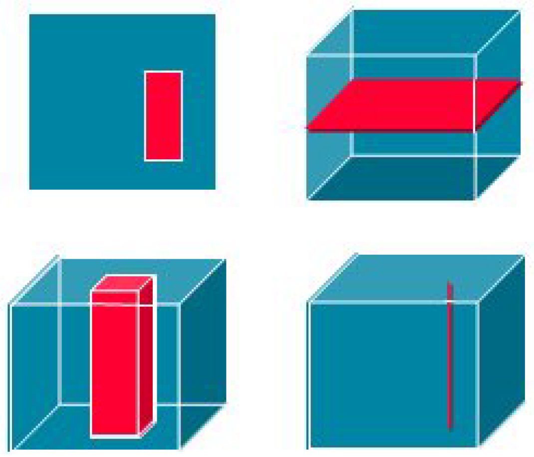
Figure 3.
A 2D and 3D visualization of OpenStreetMap (OSM) elements on a virtual globe created using NASA Web WorldWind and 3D OSM Plugin API.
Figure 3.
A 2D and 3D visualization of OpenStreetMap (OSM) elements on a virtual globe created using NASA Web WorldWind and 3D OSM Plugin API.
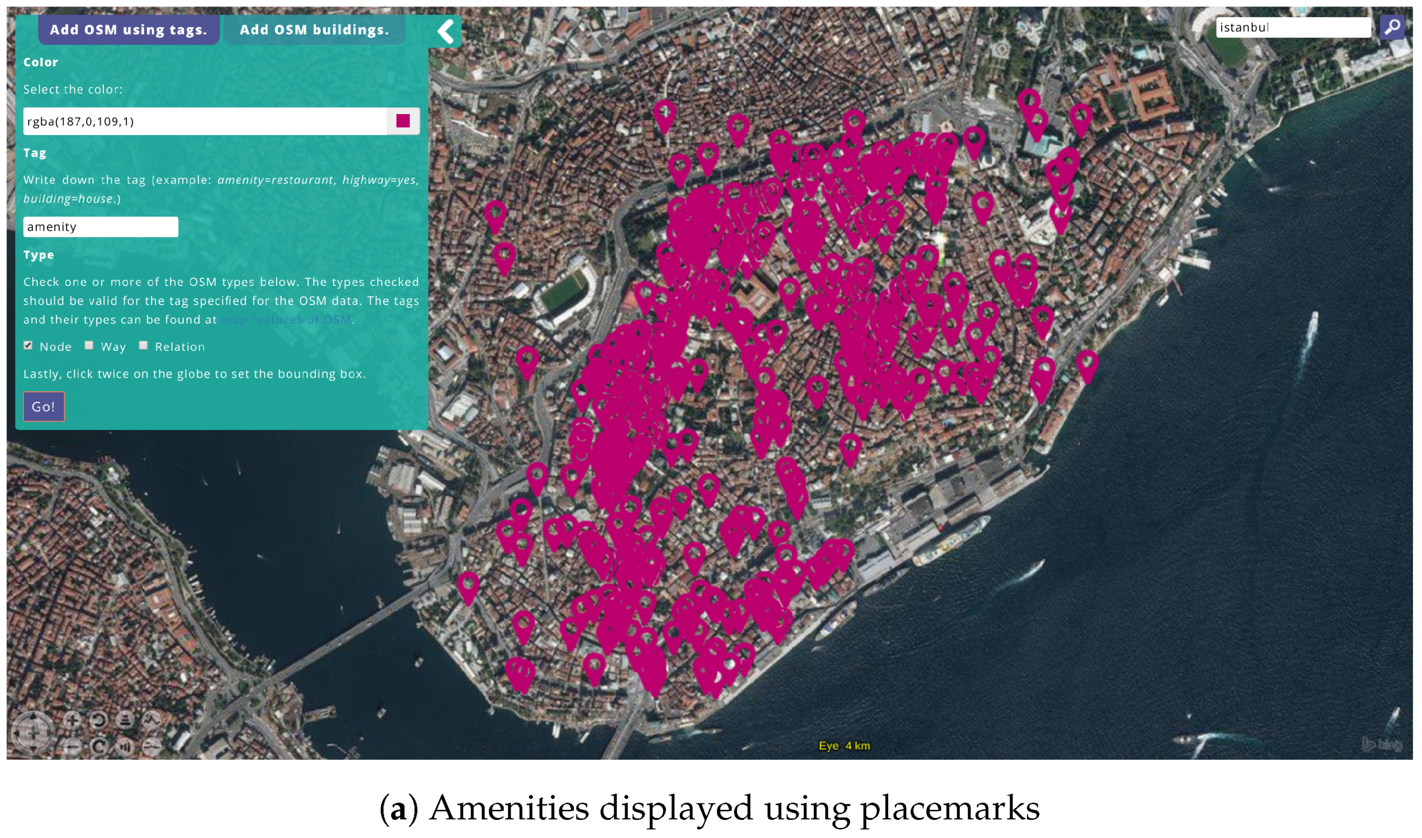

Figure 4.
Workflow for the visualization of CityGML data on a virtual globe created using CesiumJS.
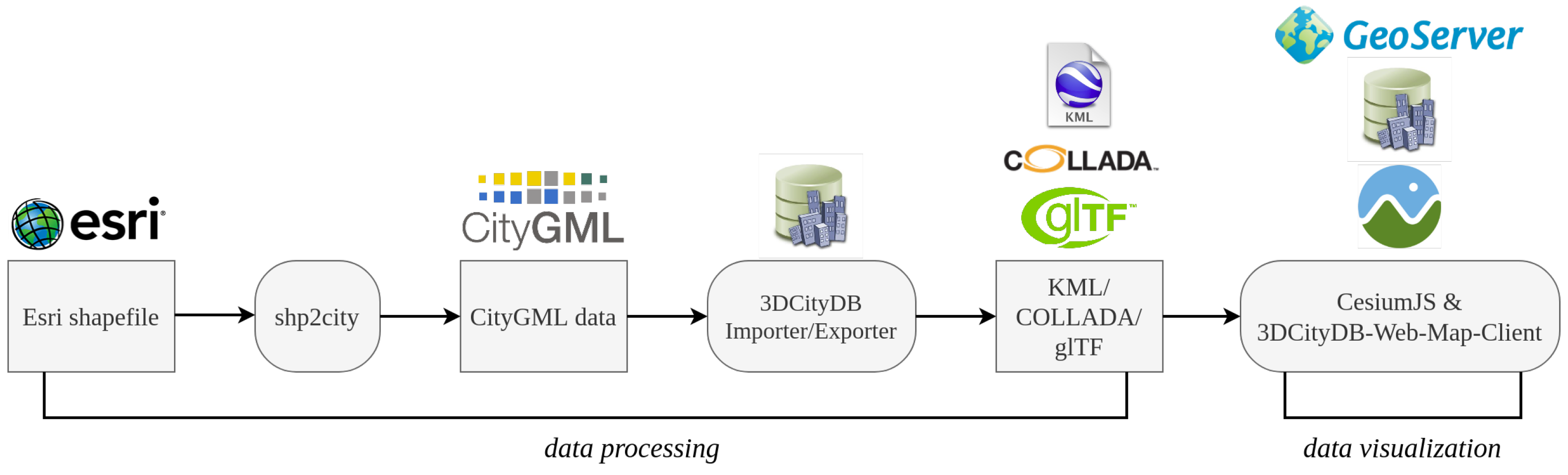
Figure 5.
Flood simulation in Milan with flood risk map and the visualization of CityGML data on a virtual globe created using CesiumJS.
Figure 5.
Flood simulation in Milan with flood risk map and the visualization of CityGML data on a virtual globe created using CesiumJS.

Figure 6.
Visualization of mean deformation velocity maps of Milan, Padua, Turin, Naples and Rome, in order from top-left to bottom, on GET-IT.
Figure 6.
Visualization of mean deformation velocity maps of Milan, Padua, Turin, Naples and Rome, in order from top-left to bottom, on GET-IT.

Figure 7.
Visualization of mean deformation velocity map of Rome and plot of cumulative deformation time series of a deformation point on a virtual globe created using CesiumJS.
Figure 7.
Visualization of mean deformation velocity map of Rome and plot of cumulative deformation time series of a deformation point on a virtual globe created using CesiumJS.

Figure 8.
Visualization of the raster deformation time series of Turin on GeoServer.

Figure 9.
Visualization of the raster file of 2005 from the raster deformation time series of Turin on a virtual globe created using CesiumJS.
Figure 9.
Visualization of the raster file of 2005 from the raster deformation time series of Turin on a virtual globe created using CesiumJS.

Figure 10.
Visualization of GHS-BUILT zoomed on Rome of 1975, 1990, 2000 and 2014, in order from top-left to bottom-right, on a virtual globe created using CesiumJS.
Figure 10.
Visualization of GHS-BUILT zoomed on Rome of 1975, 1990, 2000 and 2014, in order from top-left to bottom-right, on a virtual globe created using CesiumJS.

Figure 11.
Query of a pixel of GlobeLand30 for 2000 and 2010 on a virtual globe created using CesiumJS.
Figure 11.
Query of a pixel of GlobeLand30 for 2000 and 2010 on a virtual globe created using CesiumJS.

Figure 12.
Display of the result of the processing of the drawn area of the land consumption maps from the Italian Institute for Environmental Protection and Research (ISPRA) that calculates the amount of change of consumed areas from 2012 to 2017 on a virtual globe created using CesiumJS.
Figure 12.
Display of the result of the processing of the drawn area of the land consumption maps from the Italian Institute for Environmental Protection and Research (ISPRA) that calculates the amount of change of consumed areas from 2012 to 2017 on a virtual globe created using CesiumJS.

Figure 13.
Clusters of volunteered geographic information (VGI) on a virtual globe created using CesiumJS.
Figure 13.
Clusters of volunteered geographic information (VGI) on a virtual globe created using CesiumJS.

Figure 14.
Visualization of traffic in Rome between 12:00 and 13:00 UTC on a virtual globe created using CesiumJS.
Figure 14.
Visualization of traffic in Rome between 12:00 and 13:00 UTC on a virtual globe created using CesiumJS.
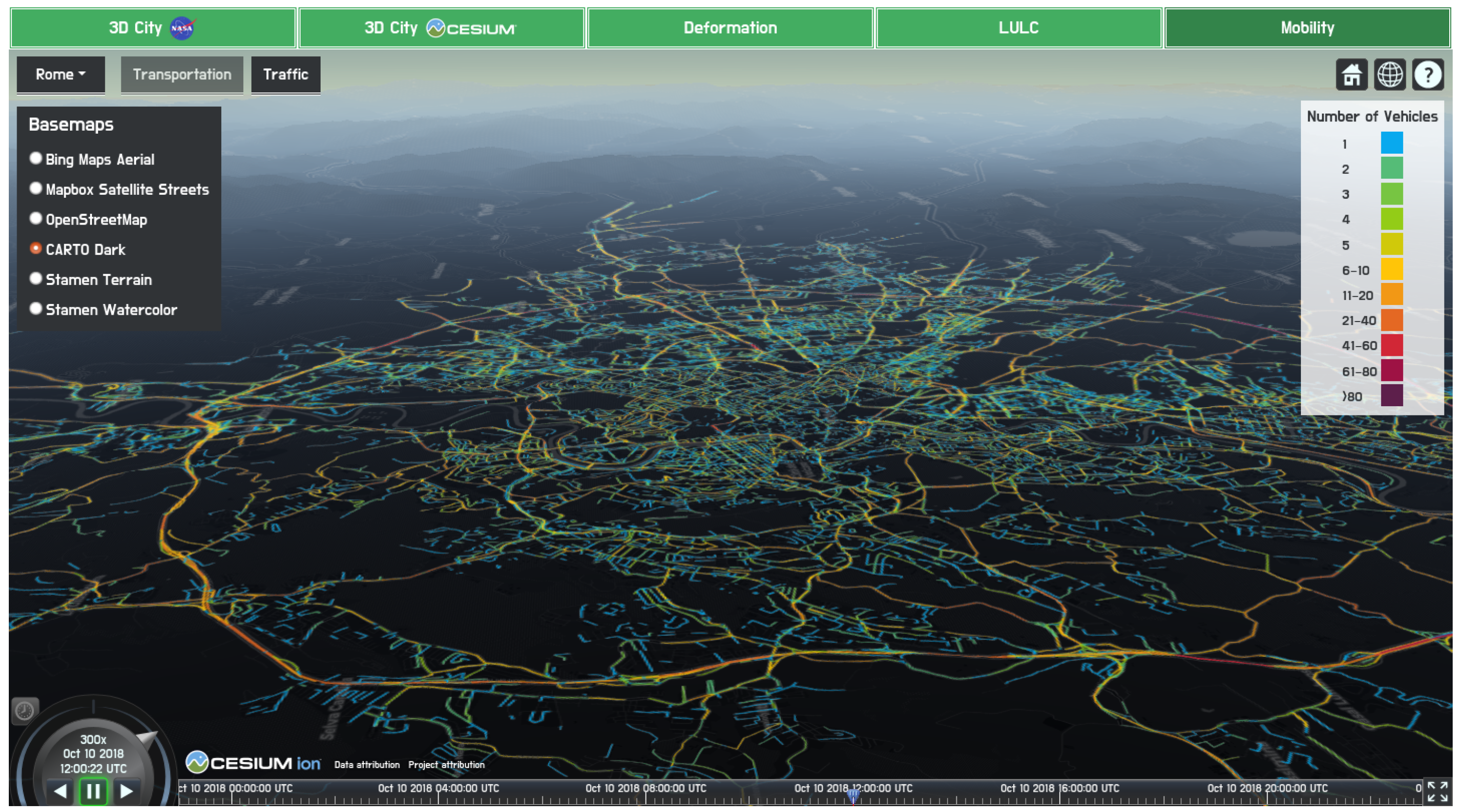
© 2020 by the authors. Licensee MDPI, Basel, Switzerland. This article is an open access article distributed under the terms and conditions of the Creative Commons Attribution (CC BY) license (http://creativecommons.org/licenses/by/4.0/).
Share and Cite
MDPI and ACS Style
Kilsedar, C.E.; Brovelli, M.A. Multidimensional Visualization and Processing of Big Open Urban Geospatial Data on the Web. ISPRS Int. J. Geo-Inf. 2020, 9, 434. https://0-doi-org.brum.beds.ac.uk/10.3390/ijgi9070434
AMA Style
Kilsedar CE, Brovelli MA. Multidimensional Visualization and Processing of Big Open Urban Geospatial Data on the Web. ISPRS International Journal of Geo-Information. 2020; 9(7):434. https://0-doi-org.brum.beds.ac.uk/10.3390/ijgi9070434
Chicago/Turabian StyleKilsedar, Candan Eylül, and Maria Antonia Brovelli. 2020. "Multidimensional Visualization and Processing of Big Open Urban Geospatial Data on the Web" ISPRS International Journal of Geo-Information 9, no. 7: 434. https://0-doi-org.brum.beds.ac.uk/10.3390/ijgi9070434
Note that from the first issue of 2016, this journal uses article numbers instead of page numbers. See further details here.