Toward Measuring the Level of Spatiotemporal Clustering of Multi-Categorical Geographic Events

Abstract

Human activity events are often recorded with their geographic locations and temporal stamps, which form spatial patterns of the events during individual time periods. Temporal attributes of these events help us understand the evolution of spatial processes over time. A challenge that researchers still face is that existing methods tend to treat all events as the same when evaluating the spatiotemporal pattern of events that have different properties. This article suggests a method for assessing the level of spatiotemporal clustering or spatiotemporal autocorrelation that may exist in a set of human activity events when they are associated with different categorical attributes. This method extends the Voronoi structure from 2D to 3D and integrates a sliding-window model as an approach to spatiotemporal tessellations of a space-time volume defined by a study area and time period. Furthermore, an index was developed to evaluate the partial spatiotemporal clustering level of one of the two event categories against the other category. The proposed method was applied to simulated data and a real-world dataset as a case study. Experimental results show that the method effectively measures the level of spatiotemporal clustering patterns among human activity events of multiple categories. The method can be applied to the analysis of large volumes of human activity events because of its computational efficiency.

1. Introduction

Events of human activities are mostly associated with definable locations and time stamps of occurrence. Collected spatial and temporal information of these events may form not only spatial patterns of activities at different periods, but also the evolution of spatial processes over time [1]. Human activity events can be recorded as point data with space and time information, which have also become increasingly available due to cost-effective sensors, widely accessible Internet, and constantly advancing geospatial technology. Data on human activity events are obtained from multiple sources that are available and are waiting for new ways to analyze and interpret [2].

Spatial and spatiotemporal statistics, a family of non-graphical indicators, are commonly used to characterize spatial/spatiotemporal autocorrelation by measuring the degrees to which the objects are inter-correlated or clustered in space and over time. The spatiotemporal autocorrelation of human activity events can be used as a fundamental reference for monitoring the evolution of events to facilitate environmental impact assessment. Human activity events, which have been studied for their levels of spatiotemporal autocorrelation, include sightings of endangered/threatened animal habitats or plant communities, crimes, inter-regional or international trades, or even recent phenomena such as social media posts and many other forms of human behavioral dynamics [3,4,5,6,7].

In most existing studies, these methods mostly focus on evaluating the spatiotemporal autocorrelation of a single type of human activity events. Working with events with more than one type, however, has two main challenges. First, as events are often assumed to be closely related to their geographical environments, all categories of events are often considered to have similar levels of spatiotemporal clustering. However, in some cases, considering that all events are the same overlooks the connection and interactive influences between different categories of activity events. Thus, key factors affecting the spatiotemporal autocorrelation of a particular type of event may not be identified. Second, spatial and temporal aspects should be considered different from a physical perspective because space and time are often measured in different units. The two dimensions should not be combined into one equation directly similar to many existing methods. These issues have severely limited the development and use of spatiotemporal autocorrelation measures of human activity events.

To fill this methodological gap, a method is proposed to measure the level of spatiotemporal clustering or the spatiotemporal autocorrelation in the distribution of a set of human activity events with binary or multiple categories. We modeled the spatiotemporal relationship among events by using the Voronoi model (for spatial dimension) and a sliding-window model (for temporal dimension). This developed index characterizes the spatiotemporal distribution autocorrelation of binary or multi-categorical events. The proposed method was applied to simulated and real-world data to show its feasibility and usage.

The contributions of this article are twofold. First, a Voronoi-based sliding-window model is proposed to support spatiotemporal analysis of geographic events with multiple categorical attribute information. The model assesses the spatiotemporal autocorrelation among human activity events represented as discrete points. It can be applied to measure the levels of spatiotemporal clustering to support subsequent analysis. Second, the importance of the relationships between categories of events in the dataset is highlighted. To the best of our knowledge, it is the first index to characterize the spatiotemporal distribution autocorrelation for point data of multiple categories.

2. Literature Review

Many events have been shown to have spatial/spatiotemporal autocorrelation that may be influenced by socio-economic and/or physical environment factors at these locations [8,9,10]. We discuss previous works on spatial autocorrelation and spatiotemporal autocorrelation. As a general practice, analysis of geographic events often starts from evaluating if a certain level of spatial/spatiotemporal clustering exists among them. If such clustering is found, then we assumed that certain factors at or nearby these locations may have influenced the distribution of events to obtain such clustering patterns. If the clustering is desirable, then the next logical step would be to identify the influencing factors to promote clustering. Alternatively, if such clustering is undesired, then the identification of influencing factors requires policy-making or appropriate actions to demote the clustering level.

2.1. Spatial Pattern of Events

Methods are available for measuring the spatial autocorrelation levels among geographic events with the interval- and ratio-scale attribute information. Many studies using such methods have been conducted to find hotspots/coldspots of geographic phenomena [11,12,13,14,15,16,17,18]; thus, appropriate actions can be taken at these locations. These methods are based on spatial statistics such as Moran’s I, nearest neighbor ratio (NNR) [19], and G-statistics. In recent years, new methods have been developed to deal with large data such as estimating spatial autocorrelation with large network data [20].

These methods were designed to work with datasets, in which all data have the same category or all events are considered the same. While capable of measuring the level of spatial clustering in a set of point data that are of the same category/type, these methods are not useful when working with point data of binary or multiple categories [21].

2.2. Spatiotemporal Pattern of Events

Spatiotemporal autocorrelation refers to the correlation of events within themselves over space and through time. It reflects the degree to which events of similar properties cluster or disperse. Some recently published studies have begun to extend spatial statistics to spatiotemporal statistics. These studies include research that measured spatiotemporal autocorrelation by developing specific space–time statistics, using space–time cubes or using space–time scans [8,9,10]. These works have extended our ability from assessing the degree to which events cluster in space to measuring how events cluster in space and over time. This advancement is important because it provides a way to analyze dynamic processes that human activity events may have evolved in space and over time.

To measure the level of spatiotemporal autocorrelation in a set of geographic events, some studies have grouped events in a temporal span to calculate the spatial autocorrelation for each time period. The results are then analyzed by time series analysis [22,23,24,25]. Other studies have aggregated points into regions and used polygons as spatial analytic units to construct a spatial adjacency structure of polygons associated with the frequencies of points in the polygons. For example, [26] used this approach to design a spatial autoregressive model for ecological studies. Other examples used housing prices as a spatiotemporal attribute associated with a set of house locations to examine spatiotemporal changes in housing prices [3,27,28]. In these and many other cases, events were clustered spatiotemporally because their characteristics were assumed to be influenced by the local conditions of their environment. Evidently, the temporal effects of influential factors are unaccounted when using only methods for measuring spatial autocorrelation. Analytical results would likely be considered and valid only as spatial events [29].

Some works have attempted to identify spatiotemporal autocorrelation of human activity events on the basis of multivariate analysis methods such as the development and application of global spatiotemporal Moran’s I by using separately structured spatial weights and temporal weights [30,31,32,33,34,35,36,37] or space–time calendar [38]. These indices have been used to measure the level of spatiotemporal autocorrelation in some geographic phenomena [32,39,40,41]. However, space and time integration should be considered more carefully.

From a physical perspective, it would make no sense to consider spatial and temporal properties of events in the same way. This is because there are significant differences between how events are related to each other in space and in time [42]. For example, two events may have a mutually influencing association in space as described in spatial interaction models. However, previous events may influence current events, but not vice versa. Therefore, the direct integration of spatial and temporal dimensions of geographic data should be carefully reconsidered. For example, the level of spatiotemporal clustering in a set of events may be considered as being created by stochastic processes [28,43], if the occurrences are assumed to have certain levels of randomness. R-tree is utilized to define spatiotemporally neighboring points and evaluate spatiotemporal Ripley’s K index [44]. In another study on the spatiotemporal trends of events, spatial autoregressive models were used for data with spatial and temporal attributes [26].

These studies evaluated the levels of spatiotemporal autocorrelation of single category of events. Our study aimed to examine and measure the levels of spatiotemporal distribution autocorrelation of one category of events when they coexist with events of other categories.

3. Method

To better understand and measure the level of spatiotemporal distribution autocorrelation of human activity events, a new method, distribution autocorrelation of human activity events (DAE) is proposed. This method is particularly useful when, for example, the studied events have multiple types or categories. As an example, criminal events in a region over a certain time period are different, for example, they can be business or residential burglaries, murders, or theft. The DAE of burglary cases is an index that measures the autocorrelation level of distribution of the burglary cases by considering all other types of crime cases as other types of crime events.

In most spatial statistics, measuring spatiotemporal autocorrelation among a set of events can be tested against a null hypothesis that assumes that events are not clustered. If an index that measures the level of spatiotemporal autocorrelation is statistically significantly different from a level representing random spatiotemporal distribution, it is said that the measured level of spatiotemporal autocorrelation is statistically significant to support the rejection of this null hypothesis.

3.1. Voronoi-Based Sliding Window Model

One way to partition a space occupied by a set of points (events) is to construct Thiessen polygons [45,46,47,48] (also known as Voronoi polygons) using points as polygon centroids. Each polygon has one point that serves as the polygon’s centroid. Any location within a Thiessen polygon is closer to the polygon’s centroid than to those of any other polygons. Spatially, Thiessen neighbors can be determined by constructing a Delaunay triangulation that connects all points into a mesh of triangles whose internal angles are maximized. If two points (centroids) are linked by an edge of a Delaunay triangle, the two points are considered Thiessen neighbors, indicating that they are centroids of two adjacent Thiessen polygons (they share at least a segment of polygon boundaries). Edges of Thiessen polygons can be drawn by perpendicular bisectors of Delaunay triangle edges. Such bisectors are then reassembled to form Thiessen polygons. The diagram of Thiessen polygons is known as a Voronoi diagram, and the way a space is partitioned into Thiessen polygons is referred to as Thiessen tessellation. In most spatial statistics that analyze points, Thiessen tessellation is used for building the spatial neighborhood structure among events that are represented as points.

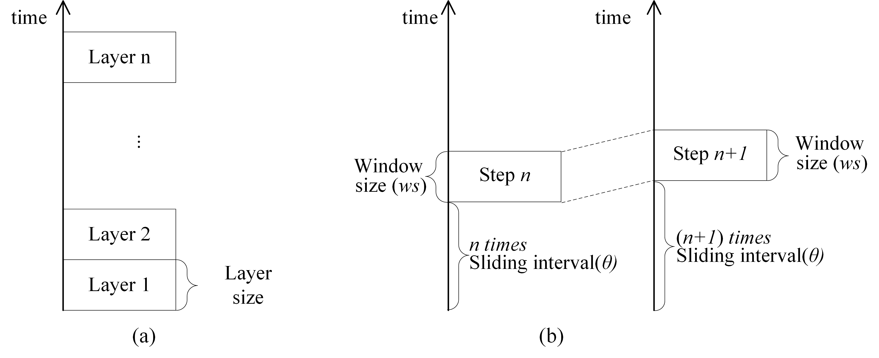
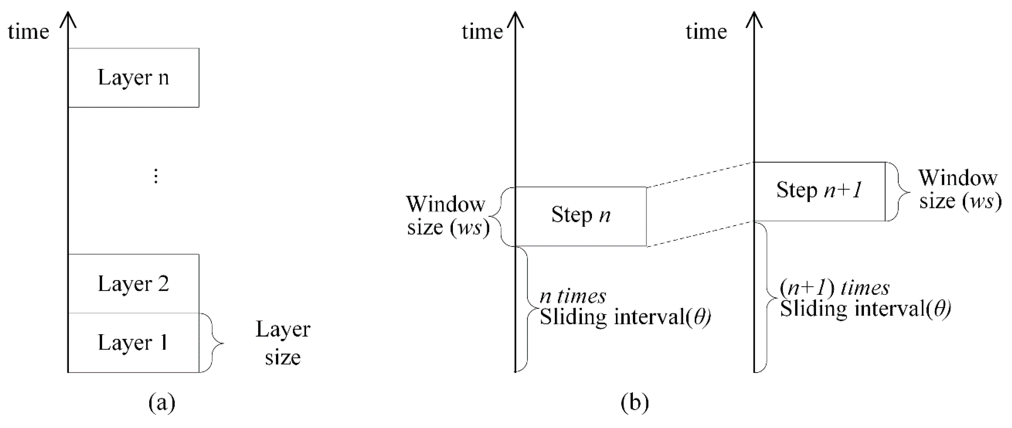
Given the properties and analytical units, where spatial and temporal relationships among event points are different, the direct integration of spatial and temporal weights by simply multiplying the spatial weights matrix and the temporal weights matrix leaves much room for debate [42]. Therefore, we cannot determine if any given pair of events are spatiotemporal neighbors by simply extending the Voronoi diagram for all events from 2D to 3D directly (for example, temporal neighborhood relationships are not mutually true while spatial neighborhood relationships may be). One possible solution to the issue of existing studies is to split events into a series of continuing time spans referred to as a layered model (Figure 1a), with each span of time considered a temporal layer.

The layered model experiences a potential difficulty, as follows: if grouping events by months and two events occurred right around the end of a month (for example, on 31 January 2019 and 1 February 2019), then they would be in different layers. Evidently, the two events should be temporally adjacent, but the layered model would separate them into two different layers. To avoid this problem, we defined a sliding-window model, as shown in Figure 1b, by dynamically itemizing the event in a layer. Given a span of time such as one week as the size of the sliding window ws, and a layer structure as described in Figure 1b, the sliding of the time window, with a sliding interval θ, starts from the bottom and proceeds upward.

We developed a new model, namely, the Voronoi-based sliding window model by combining the sliding window model and the Voronoi model. It is used to construct a spatiotemporal neighborhood structure. In the model, window sliding is repeated over the entire time duration to find spatiotemporally adjacent events on the basis of a spatial Voronoi structure. The complete algorithm is shown in Algorithm 1:

Algorithm 1. Building spatiotemporal weight matrix by sliding window algorithm.

INPUT: n = number of events, coords = locations of events, ts = occurrence time of events, ws = window size, θ = sliding step size OUTPUT: Spatiotemporal weight matrix 1: create spatiotemporal weight matrix with size of n*n and set all elements to 0 2: while the time of the latest events>= update edge of current windows 3: xs = [ ], ys = [ ] 4: for each event located in current windows 5: add x and y coordinates of event to xs and ys 6: end for 7: tri = Delaunay(xs, ys) 8: for simplices in tri: 9: for each two vertices in simplices 10: set to 1 for adjacent of the two vertices into spatiotemporal matrix 11: end for 12: end for 13: slide window with a step size θ 14: end while 15: return matrix

3.2. Evaluating the Distribution Autocorrelation of Human Activity Events (DAE) of Events

After building the structure of the spatiotemporal association among human activity events, we calculated the DAE by extending Joint Count statistics [49], a spatial statistics applicable for polygonal data with binary or multi-categorical attributes.

Let the targeted category of events be “black” and the other category of events “red”. With such marking, we can directly evaluate their DAE on the basis of Joint Count statistics. Joint Count statistics is perhaps the simplest statistical measure of spatial autocorrelation of a set of binary or multi-categorical polygons, especially when only categorical; attribute information is available to describe the characteristics of events and when the numbers of polygons in each category vary greatly. Joint Count statistics can be an excellent tool for solving the problem of measuring autocorrelation between two categories of events. Considering spatiotemporal events with a categorical attribute (such as being marked as black and red), an extended Joint Count statistic can be calculated using the number of joins between spatiotemporally neighboring events. Please note that the polygons in spatial Joint Count statistics are extended to space–time volumes in spatiotemporal Joint Count statistics. Specifically, the boundary segment between two spatially adjacent polygons is called a join. A join can be the boundary between two black polygons, between two red polygons, or between a black polygon and a red polygon. To keep things simple, we still refer to the boundary facet between two spatiotemporally adjacent volumes as a join.

The possible categories of joins, in the case of binary categories of black and red, are Black–Black, Black–Red or Red–Black, and Red–Red (where Black or Red refers to a volume of black property or a volume of red property).

Let J be the number of Black–Black joins. An index R is defined to identify the DAE for ‘Black’ events, as in Equation (1):

$$\mathrm{R}=\frac{\mathrm{J}-{\mathrm{kp}}^2}{\mathrm{S}}$$

(1)

where k is the number of all events (i.e., volumes); p is the ratio of J to k; and S is the standard errors of such expected numbers of Black–Black joins. If following the normality assumption, which assumes that the probability of any given volume being Red or Black follows a random process, then the value of the standard errors can be calculated following a probability density function with properties of a normal distribution, as follows:

$$\mathrm{S}=\sqrt{{\mathrm{kp}}^2+2{\mathrm{mp}}^3-\left(\mathrm{k}+2\mathrm{m}\right){\mathrm{p}}^2}$$

(2)

m denotes the following:

$$\mathrm{m}=\frac{1}{2}{\displaystyle \sum }_{\mathrm{i}=1}^{\mathrm{n}}{\mathrm{k}}_{\mathrm{i}}\left({\mathrm{k}}_{\mathrm{i}}-1\right)$$

(3)

The distribution autocorrelation and its statistical significance of the distribution of one category of events are determined by the value of R. If R is positive, then the assessed activity category is more spatiotemporally clustered than that of the events of other categories. Similar to most spatial statistics, the index value of R alone is not useful. A level of statistical significance should accompany this index value. In this case, the statistical significance of R is calculated using the Z-score formulation, and the associated probability density function follows a normal distribution. For example, the distribution autocorrelation is significantly clustered at the 0.05 level when the value of R is greater than 1.96, and the distribution autocorrelation is dispersed at the 0.05 level when the value of R is less than −1.96.

Finally, the level of significance test is a two-tailed test of the null hypothesis (without spatiotemporal autocorrelation) given that R can be either positive or negative.

4. Experiments and Results

4.1. Data

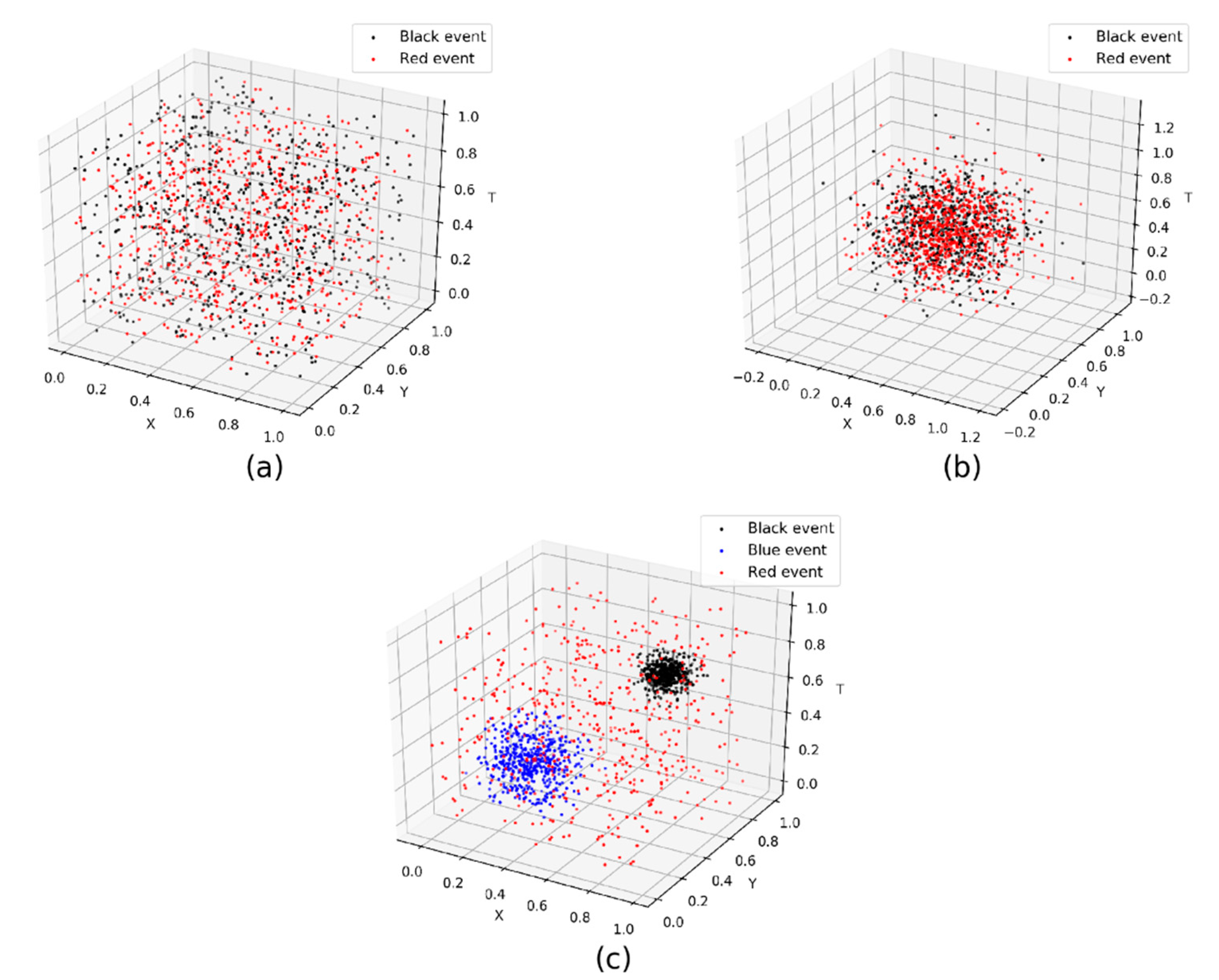
To fully evaluate the proposed method (DAE), we designed three groups of simulated data. Each data group had 1500 events. The positions of each event were defined by their x, y, and t coordinates, where (x, y) defines a spatial location, and t defines a time stamp.

In group 1, the events were created based on randomization assumption whose x, y, and t coordinates were randomly distributed between 0 and 1. The activity events were assigned to be “black” or “red” by a random process. In group 2, the events were created based on normalization assumption centered on (0.5, 0.5, 0.5) with standard deviations of coordinates set to 0.2. The events were assigned to “black” or “red” by a random process. In group 3, the events consisted of three categories, which were created based on binomial distribution assumption. The first category of events marked with “black” were distributed around (0.7, 0.7, 0.7) with a standard deviation of 0.05. The second category of events marked with “blue” were distributed around (0.3, 0.3, 0.3) with a standard deviation of 0.1, and the third category events, whose x, y, and t were randomly distributed between 0 and 1, were marked “red.” To enable comparative examinations, the number of events of each category in each group was kept the same. A set of examples for the spatiotemporal distribution of events in each group is illustrated in Figure 2a–c.

4.2. Experiment Setting

The experiments adopted Moran’s I [11,41] and nearest neighbor ratio (NNR) [50] as baseline methods to be compared with the DAE. Moran’s I is a widely used coefficient that measures the overall spatial autocorrelation of a dataset. The higher value of the coefficient means a higher spatial autocorrelation among the events in the region. NNR is calculated as the ratio of the observed average distance between nearest neighboring events to the expected average distance based on a hypothetical random distribution with the same number of features covering the same total area. It is a basic tool to examine clustering of a set of discrete points. The value of NNR varies from 0 (completely clustered) to 1 (random) to 2.149 (completely dispersed). In this paper, the two models and the proposed method (DAE) made up six indices to examine the effectiveness of the proposed method.

For the classic Moran’s I that measured the level of spatial autocorrelation among data points, the experiment initially excluded the temporal attribution of activity events. It initially divided the space into a 10 by 10 grid of 100 same sized (0.1 × 0.1) cells. The number of events inside each grid cell was considered an attribute of the grid cell. Subsequently, we considered each grid cell as a region and calculated Moran’s I value of the grid.

For spatiotemporal Moran’s I [41] that measured the spatiotemporal autocorrelation of the time–space cubic, the experiment divided the activity space into a 10 by 10 by 10 cubic volume of 1000 same size (0.1 × 0.1 × 0.1) cubes. Similarly, the number of events falling in each cube was used as its attribute. Finally, we considered each cube a volume and examined the Moran’s I of each cube.

For the classic NNR, the experiment set the parameter of the study “area” to 1, and then the ratio was calculated in accordance with the x and y coordinates of those events.

For the spatiotemporal NNR, this was derived from the classical NNR by extending spatial distance in the model to space–time distance. The distance between event a(x1, y1, t1) and event b(x2, y2, t2) was calculated using the Euclidean distance (i.e., distance(a,b) = sqrt((x2 − x1)² + (y2 − y1)² + (t2 − t1)²). Subsequently, the ratio was calculated by setting the size of the study area to 1.

For the proposed DAE method, we conducted the experiments after setting the parameter ws (windows size) into 1 and 0.2 in each of the two experiments. When ws was set to 1, all the events were located in the same time window, and the index was inclined to evaluate the spatial distribution autocorrelation of events than the spatiotemporal distribution autocorrelation.

We performed a 100-permutation test to evaluate the accuracy values of the six indices, and the median value of R and p-value in each group were recorded as the group’s result.

4.3. Results

As mentioned in Section 4.1, the “black” events in group 2 and group 3 and “blue” events in group 3 were three cases, whose distributions were simulated with the normalization assumption. The result of Moran’s I and ST Moran’s I of the three cases showed that those events were autocorrelated at the 0.001 significance level. All values of NNR and ST NNR of the three cases were greater than 0 and were statistically significant at the 0.05 level. In other words, the four indices had successfully identified the normalization autocorrelation, whereas the “black” event in group 1 and the “red” events in group 3 were two cases that were simulated with the randomization assumption. The four indices, Moran’s I, ST Moran’s, NNR, and ST NNR were very close to 0, indicating that they measured the levels of autocorrelation among the events effectively. In summary, the four indices had obtained reasonable values when measuring the levels of spatial/spatiotemporal autocorrelation. However, their shortcoming was that they could not identify the difference of distribution autocorrelation between two category events, called partial autocorrelation. The concept of partial autocorrelation is similar to the partial regression coefficient in a multivariate regression model; it measures the autocorrelation of events of a particular category while considering all events of other categories as the second type. The lack of means to calculate partial autocorrelation could be a limitation of the classical methods; thus, we were motivated to carry out this study.

It should be noted that even in evaluating absolute (as opposed to partial) spatiotemporal autocorrelation, the spatiotemporal NNR has some limitations. Its R values should be approximately 1 for the “black” events subgroup in group 1 and for the “red” events subgroup in group 3 because the “black” events were simulated to be randomly distributed. The R’s should be less than 1 for the “black” subgroup events in group 2 because the distribution of data was simulated with the normalization assumption. Furthermore, they should have a p-value of at least 0.05 in the three subgroups because the distribution autocorrelation of the events in three subgroups was not statistically significant.

According to

Table 1. Results in three group data (the ST in the table denotes spatiotemporal).

Index	“Black” in Group 1		“Black” in Group 2		“Black” in Group 3		“Blue” in Group 3		“Red” in Group 3
	R	p-Value	R	p-Value	R	p-Value	R	p-Value	R	p-Value
Moran’s I	−0.00	0.44	0.76	0.00	0.38	0.00	0.64	0.00	−0.01	0.83
ST Moran’s I	0.00	0.50	0.60	0.00	0.29	0.00	0.55	0.00	−0.00	0.47
NNR	1.00	0.30	0.96	0.01	0.23	0.00	0.48	0.00	1.02	0.17
ST NNR	0.19	0.00	1.67	0.00	0.34	0.00	0.70	0.00	1.62	0.00
R(ws = 1)	0.14	0.44	0.18	0.42	22.24	0.00	17.69	0.00	15.01	0.00
R(ws = 0.2)	−0.11	0.54	0.05	0.47	24.75	0.00	21.46	0.00	15.64	0.00

, the proposed DAE method successfully evaluated the distribution of the target category of events against other categories of events. When the target events had similar distributions in different groups, the spatiotemporal R was extremely low, with approximately 0.5 p-value on the “black” event subgroups in group 1 and group 2. The events of three subgroups in group 3 had different levels of distribution autocorrelation: a high R value indicated that the target category was distributed differently from those of other categories. In addition, the three R’s decreased gradually along with the decrease in the degrees of aggregation of three categories of events.

5. Discussion

5.1. Impact of the Target Activity Ratio

To examine whether the ratio of target events against others would affect the calculated index values, we assumed that the data were under three different distributions: random, standard normal distribution, and binormal distribution, and repeated the experiments with ratios of “black” being set from 0.1 to 0.9 (i.e., 10% and 90% of all event points in a simulated dataset). For each experiment, the size of the sliding window (ws) was set to 0.1, the sliding interval θ was set to 0.01, and the number of permutations was set to 100. The median of the obtained index values and their corresponding p-values are listed in

Table 2. Impact of black ratio with Voronoi-based sliding window model.

% Black	Random Distribution		Normal Distribution		Binomial Distribution
	R	p-Value	R	p-Value	R	p-Value
0.1	−0.05	0.52	−0.14	0.55	32.04	0.00
0.2	0.13	0.44	0.09	0.46	27.35	0.00
0.3	−0.07	0.52	0.03	0.48	22.68	0.00
0.4	−0.02	0.51	−0.02	0.51	19.71	0.00
0.5	−0.05	0.52	−0.00	0.50	16.39	0.00
0.6	−0.00	0.50	−0.04	0.51	13.60	0.00
0.7	−0.01	0.50	−0.06	0.52	10.97	0.00
0.8	0.02	0.49	−0.02	0.50	8.62	0.00
0.9	−0.00	0.50	0.01	0.49	5.72	0.00

.

Table 2 shows that all R values were very close to 0, but none were significantly different in the proportions of “black” events in data under either randomization or normalization assumptions. In group 3, binomial distribution, the R values decreased from 15.664 to 4.037, whereas the proportions of “black” events increased from 0.1 (10%) to 0.9 (90%) in the simulated datasets. This finding is due to the number of events marked “black” being greater than half of the total numbers of all events. This was not the case, however, when the number of one category was less than the total number of other categories of activities.

5.2. Impact of the Size Sliding Window Size and Step Size

Using the DAE model, the size of the sliding windows (ws) and step size (θ) should have some impacts on R values. Considering that the distribution of “black” data in group 3 was significant with all six indices, we used the same simulated data of group 3 in Section 4 to conduct more experiments to verify the influence of window size and step size. The values of ws used in the experiments started from 0.05 to 0.5 with increment θ from 0.005 to 0.05. The median R values of each 100 permutations are listed in

Table 3. (a) The R values with different windows sizes (ws) and different step sizes (θ) for the group 3 data, where R_0.005 denotes the obtained values of Rs when θ is set to 0.005. (b) The deviation matrix compared to the baseline result.

a
ws	R0.005	R0.010	R0.015		R0.020	R0.025	R0.030	R0.035	R0.040	R0.045	R0.050	Avg.
0.05	21.17	21.23	20.96		20.67	20.67	20.28	19.65	19.56	19.84	20.20	20.67
0.10	21.09	21.21	21.09		21.19	21.13	21.13	21.09	21.07	21.01	21.19	21.13
0.15	21.19	21.08	21.32		21.10	21.30	21.21	20.99	21.10	21.16	21.10	21.10
0.20	21.12	21.20	21.18		21.27	21.17	20.84	21.12	21.00	20.76	21.08	21.12
0.25	20.61	20.66	20.80		20.84	20.82	20.70	20.93	20.93	20.70	20.92	20.80
0.30	19.70	19.71	19.89		20.00	19.99	20.04	20.07	20.25	20.16	20.21	20.00
0.35	18.55	18.68	18.88		18.87	18.83	18.90	19.09	19.50	19.38	19.03	18.88
0.40	17.69	17.77	17.83		18.00	18.04	18.13	18.38	18.20	18.41	18.17	18.04
0.45	16.86	16.88	17.05		16.99	17.16	17.12	17.43	17.40	17.56	17.59	17.12
0.50	16.55	16.55	16.73		16.72	16.71	16.66	16.66	16.88	16.88	16.99	16.71
Avg.	19.45	19.50	19.57		19.56	19.58	19.50	19.54	19.59	19.59	19.65	19.50
b
ws	R0.001	D0.005	D0.010	D0.015	D0.020	D0.025	D0.030	D0.035	D0.040	D0.045	D0.050	Avg.
0.05	21.07	0.10	0.16	0.11	0.40	0.41	0.79	1.42	1.52	1.23	0.87	0.41
0.10	21.24	0.15	0.03	0.15	0.04	0.11	0.11	0.15	0.17	0.23	0.04	0.11
0.15	21.07	0.13	0.01	0.25	0.03	0.23	0.14	0.07	0.04	0.10	0.04	0.04
0.20	20.54	0.58	0.66	0.64	0.73	0.63	0.30	0.57	0.46	0.22	0.54	0.57
0.25	19.75	0.86	0.91	1.05	1.10	1.08	0.96	1.19	1.18	0.96	1.18	1.05
0.30	18.60	1.10	1.10	1.28	1.39	1.39	1.44	1.46	1.65	1.55	1.60	1.39
0.35	17.75	0.79	0.92	1.12	1.11	1.07	1.14	1.34	1.75	1.63	1.27	1.12
0.40	17.05	0.63	0.72	0.78	0.94	0.98	1.08	1.33	1.15	1.36	1.11	0.98
0.45	16.37	0.49	0.51	0.67	0.61	0.79	0.75	1.05	1.02	1.18	1.21	0.75
0.50	16.55	0.00	0.00	0.18	0.17	0.16	0.12	0.11	0.34	0.33	0.44	0.16
Avg.	19.00	0.48	0.50	0.62	0.65	0.69	0.68	0.87	0.93	0.88	0.83	0.66

a.

Table 3a shows that the window size was significantly correlated to the results. It should be noted that bias could exist because the spatial distribution of x, y and temporal distribution t were very similarly controlled and generated by the same assumption and parameters.

However, there was no clear evidence showing that the results were connected to step size. Ideally, θ should be as small as possible so that the window moves smoothly and therefore would better capture the temporal and spatial relationships between events. To better examine the impact of step size, we took a very small θ, 0.001, as a baseline θ. Then, we took D_x to present the deviation between the values of R in the baseline and of R_x, which was obtained when θ was set to x. The D_x was calculated by |R_0.001 − R_x|, as listed in Table 3b.

As shown in Table 3b, as the θ increased, so did the average of D_θ. A smaller D_θ means that the values of R had less deviation with the theoretical results, and was thought to be better. It suggests that the proposed index prefers that θ should be as small as possible. However, a smaller θ requires repeating the Delaunay process more, which is time consuming.

We believe that ws will cause an MTUP (modifiable temporal unit problem). For events from the real world, natural units of time such as a year, month, week, day, would be good choices for ws. In addition, the time span of all events should cross dozens of ws for fine capturing the temporal impact. For θ, the smaller the better.

5.3. Performance Analysis

Since event data are increasingly generated and made available, new models and methods are required to handle large volumes of event data. To investigate the relationship between the cost of computation time and the volumes of event data, we conducted experiments using four sample datasets of different sizes consisting of 1000 events, 10,000 events, 100,000 events, and 1,000,000 events, respectively. The times used in calculating the three indices of ST Moran’s I, ST NNR, and the proposed index (R) were recorded and presented in

Table 4. The computation time (seconds) of different sample size for three ST models, where NA represents the computation process is not finished within 10 h (36,000 s).

Index	n = 1000	n = 10,000	n = 100,000	n = 1,000,000
ST Moran’s I	0.24	229.69	20387.89	NA
ST NNR	0.03	0.70	191.26	NA
R(ws = 0.2, θ = 0.01)	1.44	13.66	140.00	1497.30
R(ws = 0.2, θ = 0.02)	0.71	6.98	75.45	704.94
R(ws = 0.1, θ = 0.01)	0.76	7.48	71.51	704.18
R(ws = 0.1, θ = 0.02)	0.34	3.16	32.41	349.99

.

As shown in Table 4, the computation times for the ST Moran’s I and ST NNR index increased rapidly as the sample size increased. In contrast, our method was more efficient at handling large amounts of data. The required time of the proposed index increased when the sample size increased, showing a linear relationship with the sample size. Moreover, the time overhead was related to the two parameters, ws and θ:

(1)

When ws was greater, more events fell into each temporal window and were involved in each Delaunay model, thus requiring more calculation time.

(2)

When the value of θ was smaller, more time for constructing the Delaunay triangulation was required, resulting in more overall computation time.

5.4. Real World Application—A Case of Call-for-Service Records

A call-for-service dataset in Portland, Oregon, with geographic coordinates and time stamps, was used in this case study. The data was downloaded from the official website of Real-Time Crime Forecasting Challenge (https://nij.gov/funding/Pages/fy16-crime-forecasting-challenge.aspx, accessed on 19 May 2017). A total of 95 categories of events were recorded in the downloaded call-for-service data, which represented 208,083 event cases located in Portland during that time.

Considering that the population may be closely related to the numbers of calls [51], the density of population and calls of per square kilometer by census tracts are mapped, as shown in Figure 3a,b, respectively. From these figures, some levels of spatial clustering in the distributions of population and calls can be observed visually.

We focused on the top 10 tracts whose call numbers were the highest among all tracts. As shown in

Table 5. Frequencies of Top-10 call categories.

Category	Case Description	Number	Percent
UNWNT	UNWANTED PERSON	24,747	11.89%
DISTP	DISTURBANCE	21,715	10.44%
SUSP	SUSPICIOUS SUBJ, VEH, OR CIRCUMSTANCE	13,481	6.48%
WELCKP	WELFARE CHECK—PRIORITY	12,673	6.09%
THEFT	THEFT—COLD	12,036	5.78%
WELCK	WELFARE CHECK—COLD	11,616	5.58%
AREACK	AREA CHECK	6444	3.10%
ASSIST	ASSIST—CITIZEN OR AGENCY	6284	3.02%
ACCNON	ACCIDENT—NON INJURY	6050	2.91%
HAZARD	HAZARD—HAZARDOUS CONDITION	5926	2.85%
		120,972	58.14

, the accumulated number of calls of the top 10 call-for-service categories was more than 50% of the total number of calls from all categories.

To examine the spatial patterns by call categories, we evaluated them by using the Moran’s I with two spatial units, namely, tracts and census block groups. In addition, nearest neighbor ratio (NNR) values were calculated using default parameters for each of the top 10 call categories. Results are shown in

Table 6. (a) Classical spatial pattern of call for service record (Znorm is the Z-score calculated under normality assumption). (b) Classical spatial pattern of call for service record (Zrand is the Z-score calculated under randomness assumption).

a
Case Type	Moran’s I Tract			Moran’s I Block Group			NNR
	Moran’s I	Znorm	p-Value	Moran’s I	Znorm	P-Value	Z	p-Value
UNWNT	0.46	9.70	0.00	0.51	19.02	0.00	−212.36	0.00
DISTP	0.32	6.84	0.00	0.47	17.54	0.00	−180.92	0.00
SUSP	0.38	8.01	0.00	0.42	15.56	0.00	−97.61	0.00
WELCKP	0.41	8.59	0.00	0.56	20.76	0.00	−120.46	0.00
THEFT	0.37	7.81	0.00	0.41	15.27	0.00	−105.45	0.00
WELCK	0.39	8.20	0.00	0.53	19.86	0.00	−112.43	0.00
AREACK	0.36	7.57	0.00	0.45	16.54	0.00	−63.02	0.00
ASSIST	0.34	7.17	0.00	0.48	17.94	0.00	−71.05	0.00
ACCNON	0.32	6.82	0.00	0.32	12.04	0.00	−87.90	0.00
HAZARD	0.30	6.36	0.00	0.31	11.67	0.00	−89.97	0.00
b
Case Type	Moran’s I Tract			Moran’s I Block Group
	Moran’s I	Zrand	p-Value	Moran’s I	Zrand	p-Value
UNWNT	0.46	10.57	0.00	0.51	20.28	0.00
DISTP	0.32	7.51	0.00	0.47	17.86	0.00
SUSP	0.38	8.42	0.00	0.42	15.52	0.00
WELCKP	0.41	9.52	0.00	0.56	22.29	0.00
THEFT	0.37	7.84	0.00	0.41	15.93	0.00
WELCK	0.39	9.05	0.00	0.53	20.27	0.00
AREACK	0.36	7.79	0.00	0.45	17.41	0.00
ASSIST	0.34	7.46	0.00	0.48	18.15	0.00
ACCNON	0.32	7.10	0.00	0.32	12.40	0.00
HAZARD	0.30	6.33	0.00	0.31	11.64	0.00

a,b.

Table 6a,b show the certainly statistically significant levels of spatial clustering with respect to all call categories. However, identifying which call category showed a spatial pattern that is significantly different from that of all call categories was difficult because all spatial patterns are statistically significantly clustered for this dataset. Therefore, analyzing these events to identify the autocorrelation distribution pattern over different call categories is necessary. We evaluated the partial spatiotemporal autocorrelation for each category of events using the proposed method, and the results are shown in

Table 7. Distribution autocorrelation of human activity events (DAE) of call for service records.

Case Type	ws = 365 Days		ws = 7 Days
	R	p-Value	R	p-Value
UNWNT	−8.69	0.00	11.43	0.00
DISTP	18.93	0.00	9.49	0.00
SUSP	28.92	0.00	12.49	0.00
WELCKP	−7.35	0.00	4.08	0.00
THEFT	6.45	0.00	5.19	0.00
WELCK	−4.62	0.00	4.46	0.00
AREACK	11.24	0.00	4.51	0.00
ASSIST	1.66	0.09	5.8	0.00
ACCNON	−1.63	0.10	12.45	0.00
HAZARD	4.26	0.00	47.41	0.00

.

Table 7 shows the remarkable difference among different call categories. The R’s of the UNWNT, WELCKP, and WELCK categories were less than 1.96. Although they were significantly clustered in space and time, they seem to be significantly dispersed when compared with those of other call categories. Such an outcome suggests that call categories with small absolute R values may not have special spatial factors that can influence the source of these calls. Alternatively, the DISTP, SUSP, THEFT, AREACK, and HAZARD categories have evident spatiotemporal relative aggregation characteristics, as shown by their partial autocorrelation measures. This finding indicates that they could be closely related to specific spatial environments and other factors. This condition is only possible when partial autocorrelation levels are calculated.

Table 6 also shows that the levels of the DAE (when ws was set to seven days) of all call categories were more statistically significant than the spatial pattern (when ws was set to 365 days) of any given call category. This finding suggests that the temporal patterns in these call events must not be overlooked.

6. Concluding Remarks

To better distinguish the distribution autocorrelation of human activity events, a new method for measuring the levels of autocorrelation in a set of events was proposed. With this method, we built a Voronoi-based sliding window model to solve the problem of finding spatiotemporal neighbors among human activity events. The model is based on integrating space and time dimensions while maintaining spatiotemporal heterogeneity among spatiotemporal events. We also analyzed and demonstrated the properties and usage of this method by applying it to simulated data and a case study of real-world data. The experimental results showed that the proposed method can examine and measure the level of spatiotemporal autocorrelation in a set of events. The results of this study are expected to enrich the spatiotemporal analysis methods of categorical events and provide a new approach for the applications of spatiotemporal analysis methods/data when working with large volumes of data on human activities.

However, this study still has some limitations that may require further research. First, using only one case study may be biased because different outcomes may be obtained when the proposed method is used in different case studies. The call-for-service records used here are only for the purpose of illustrating the methodological procedures and checking the effectiveness of the methods. More works on classifying call-for-service records to different categories may be needed by applying the proposed method to more datasets of different characteristics. Furthermore, the sliding window model lacks a means to define an optimal universal window size. In practical uses, such window sizes may depend upon the way a particular category of events being analyzed is distributed.

Along the temporal dimension, geographical events can affect other events in ways that are different from those in spatial dimensions. For example, past events may affect how current events evolve, but not vice versa. Similarly, the effects that some events may have on others may have time-delayed impacts. The current format of the method discussed in the paper does not consider these effects. Additionally, the frequencies of events should be assessed to see if they have any temporal cycles, which are important when defining an appropriate temporal window size in the analysis.

Finally, as in almost all spatial statistics, the boundary issue should also be recognized here. Conventionally, a buffer zone can be constructed to include geographic events from the neighboring areas into the dataset for analysis. That, of course, is feasible only when such data are available.

References

- Noonan, M.J.; Tucker, M.A.; Fleming, C.H.; Akre, T.S.; Alberts, S.C.; Ali, A.H.; Altmann, J.; Antunes, P.C.; Belant, J.L.; Beyer, D. A comprehensive analysis of autocorrelation and bias in home range estimation. Ecol. Monogr. 2019, 89, e01344. [Google Scholar] [CrossRef]
- Arribas-Bel, D.; Tranos, E. Big urban data: Challenges and opportunities for geographical analysis. Geogr. Anal. 2018, 50, 123–124. [Google Scholar] [CrossRef]
- Ma, W.; Ji, J.; Chen, P.; Zhao, T. Spatial-temporal patterns analysis of property crime in urban district based on Moran’s I and GIS. In Proceedings of the Information Technology and Computer Application Engineering (ITCAE 2013), Hong Kong, China, 27–28 August 2013; pp. 253–258. [Google Scholar]
- Bao, P.-M.; JI, G.-L.; Wang, C.-L.; Zhu, Y.-B. Algorithms for mining human spatial-temporal behavior pattern from mobile phone trajectories. DEStech Trans. Comput. Sci. Eng. 2017. [Google Scholar] [CrossRef] [Green Version]
- Huang, C.; Wang, D. Exploiting Spatial-Temporal-Social Constraints for Localness Inference Using Online Social Media. In Proceedings of the Advances in Social Networks Analysis and Mining (ASONAM), 2016 IEEE/ACM International Conference on, San Francisco, CA, USA, 18–21 August 2016; pp. 287–294. [Google Scholar]
- Liu, Z.; Yu, J.; Xiong, W.; Lu, J.; Yang, J.; Wang, Q. Using Mobile Phone Data to Explore Spatial-Temporal Evolution of Home-Based Daily Mobility Patterns in Shanghai. In Proceedings of the Behavioral, Economic and Socio-cultural Computing (BESC), 2016 International Conference on, Durham, NC, USA, 11–13 November 2016; pp. 1–6. [Google Scholar]
- Zhang, Y.; Fu, Y.; Wang, P.; Li, X.; Zheng, Y. Unifying Inter-region Autocorrelation and Intra-region Structures for Spatial Embedding via Collective Adversarial Learning. In Proceedings of the 25th ACM SIGKDD International Conference on Knowledge Discovery & Data Mining, Anchorage, AK, USA, 4–9 August 2019; pp. 1700–1708. [Google Scholar]
- Nakaya, T.; Yano, K. Visualising crime clusters in a space-time cube: An exploratory data-analysis approach using space-time kernel density estimation and scan statistics. Trans. GIS 2010, 14, 223–239. [Google Scholar] [CrossRef]
- Lee, J.; Gong, J.; Li, S. Exploring spatiotemporal clusters based on extended kernel estimation methods. Int. J. Geogr. Inf. Sci. 2017, 31, 1154–1177. [Google Scholar] [CrossRef]
- Tango, T. Space-time scan statistics. In Statistical Methods for Disease Clustering; Springer: Berlin/Heidelberg, Germany, 2010; pp. 211–233. [Google Scholar]
- Anselin, L. The Moran scatterplot as an ESDA tool to assess local instability in spatial association. Spat. Anal. Perspect. GIS 1996, 111, 111–125. [Google Scholar]
- Li, S.; Ye, X.; Lee, J.; Gong, J.; Qin, C. Spatiotemporal analysis of housing prices in China: A big data perspective. Appl. Spat. Anal. Policy 2017, 10, 421–433. [Google Scholar] [CrossRef]
- Lay, J.G.; Lin, Z.H.; Yap, K.H.; Wu, P.C.; Su, H.J. Temperature variability and spatial hotspots of dengue fever occurrence in Taiwan. Epidemiology 2006, 17, S485. [Google Scholar] [CrossRef]
- Manne, L.L.; Williams, P.H.; Midgley, G.F.; Thuiller, W.; Rebelo, T.; Hannah, L. Spatial and temporal variation in species-area relationships in the Fynbos biological hotspot. Ecography 2007, 30, 852–861. [Google Scholar] [CrossRef]
- Chen, Q.; Liu, G.; Ma, X.; Zhang, J.; Zhang, X. Conditional multiple-point geostatistical simulation for unevenly distributed sample data. Stoch. Environ. Res. Risk Assess. 2019, 33, 973–987. [Google Scholar] [CrossRef]
- Fu, W.; Zhao, K.; Zhang, C.; Tunney, H. Using Moran’s I and geostatistics to identify spatial patterns of soil nutrients in two different long-term phosphorus-application plots. J. Plant Nutr. Soil Sci. 2011, 174, 785–798. [Google Scholar] [CrossRef]
- Ratcliffe, J.H.; Taniguchi, T.; Groff, E.R.; Wood, J.D. The Philadelphia foot patrol experiment: A randomized controlled trial of police patrol effectiveness in violent crime hotspots. Criminology 2011, 49, 795–831. [Google Scholar] [CrossRef]
- Chaikaew, N.; Tripathi, N.K.; Souris, M. Exploring spatial patterns and hotspots of diarrhea in Chiang Mai, Thailand. Int. J. Health Geogr. 2009, 8, 36. [Google Scholar] [CrossRef] [PubMed] [Green Version]
- Clark, P.J.; Evans, F.C. Distance to nearest neighbor as a measure of spatial relationships in populations. Ecology 1954, 35, 445–453. [Google Scholar] [CrossRef]
- Zhou, J.; Tu, Y.; Chen, Y.; Wang, H. Estimating spatial autocorrelation with sampled network data. J. Bus. Econ. Stat. 2017, 35, 130–138. [Google Scholar] [CrossRef]
- Cao, G.; Kyriakidis, P.; Goodchild, M. A geostatistical framework for categorical spatial data modeling. SIGSPATIAL Spec. 2011, 3, 4–9. [Google Scholar] [CrossRef]
- Townsley, M. Visualising space time patterns in crime: The hotspot plot. Crime Patterns Anal. 2008, 1, 61–74. [Google Scholar]
- Gómez, C.; White, J.C.; Wulder, M.A. Characterizing the state and processes of change in a dynamic forest environment using hierarchical spatio-temporal segmentation. Remote Sens. Environ. 2011, 115, 1665–1679. [Google Scholar] [CrossRef]
- Cheng, T.; Haworth, J.; Wang, J. Spatio-temporal autocorrelation of road network data. J. Geogr. Syst. 2012, 14, 389–413. [Google Scholar] [CrossRef]
- Saizen, I.; Maekawa, A.; Yamamura, N. Spatial analysis of time-series changes in livestock distribution by detection of local spatial associations in Mongolia. Appl. Geogr. 2010, 30, 639–649. [Google Scholar] [CrossRef]
- Ver Hoef, J.M.; Peterson, E.E.; Hooten, M.B.; Hanks, E.M.; Fortin, M.J. Spatial autoregressive models for statistical inference from ecological data. Ecol. Monogr. 2018, 88, 36–59. [Google Scholar] [CrossRef] [Green Version]
- Dubé, J.; Legros, D. A spatio-temporal measure of spatial dependence: An example using real estate data. Pap. Reg. Sci. 2013, 92, 19–30. [Google Scholar] [CrossRef]
- Shen, C.; Li, C.; Si, Y. Spatio-temporal autocorrelation measures for nonstationary series: A new temporally detrended spatio-temporal Moran’s index. Phys. Lett. A 2016, 380, 106–116. [Google Scholar] [CrossRef]
- Griffith, D.A.; Paelinck, J.H. The Relative Importance of Spatial and Temporal Autocorrelation. In Morphisms for Quantitative Spatial Analysis; Springer: Berlin/Heidelberg, Germany, 2018; pp. 35–47. [Google Scholar]
- López, F.A.; Matilla-García, M.; Mur, J.; Marín, M.R. Four tests of independence in spatiotemporal data. Pap. Reg. Sci. 2011, 90, 663–685. [Google Scholar] [CrossRef]
- Griffith, D. Interdependence in space and time: Numerical and interpretative considerations. Dyn. Spat. models 1981, 1, 258–287. [Google Scholar]
- Cliff, A.D.; Ord, J.K. Spatial and temporal analysis: Autocorrelation in space and time. Quant. Geogr. Br. View 1981, 1, 104–110. [Google Scholar]
- Pebesma, E. Spacetime: Spatio-temporal data in r. J. Stat. Softw. 2012, 51, 1–30. [Google Scholar] [CrossRef] [Green Version]
- Cressie, N.; Wikle, C.K. Statistics for Spatio-Temporal Data; John Wiley & Sons: Hoboken, NJ, USA, 2015. [Google Scholar]
- Chen, Y. An analytical process of spatial autocorrelation functions based on Moran’s Index. arXiv 2020, arXiv:2001.06750. [Google Scholar]
- Gao, Y.; Cheng, J.; Meng, H.; Liu, Y. Measuring spatio-temporal autocorrelation in time series data of collective human mobility. Geo Spat. Inf. Sci. 2019, 22, 166–173. [Google Scholar] [CrossRef] [Green Version]
- Souris, M.; Demoraes, F. Improvement of spatial autocorrelation, kernel estimation, and modeling methods by spatial standardization on distance. ISPRS Int. J. Geo Inf. 2019, 8, 199. [Google Scholar] [CrossRef] [Green Version]
- Arribas-Bel, D.; Tranos, E. Characterizing the spatial structure(s) of cities “on the fly”: The space-time calendar. Geogr. Anal. 2018, 50, 162–181. [Google Scholar] [CrossRef]
- Nakhapakorn, K.; Jirakajohnkool, S. Temporal and spatial autocorrelation statistics of dengue fever. Dengue Bull. 2006, 30, 177–183. [Google Scholar]
- Gottwald, T.; Reynolds, K.; Campbell, C.; Timmer, L. Spatial and spatiotemporal autocorrelation analysis of citrus canker epidemics in citrus nurseries and groves in Argentina. Phytopathology 1992, 82, 843–851. [Google Scholar] [CrossRef]
- Lee, J.; Li, S. Extending Moran’s Index for measuring spatiotemporal clustering of geographic events. Geogr. Anal. 2017, 49, 36–57. [Google Scholar] [CrossRef]
- Mateu, J.; Müller, W.G. Spatio-Temporal Design: Advances in Efficient Data Acquisition; John Wiley & Sons: Hoboken, NJ, USA, 2013. [Google Scholar]
- Geniaux, G.; Martinetti, D. A new method for dealing simultaneously with spatial autocorrelation and spatial heterogeneity in regression models. Reg. Sci. Urban Econ. 2017. [Google Scholar] [CrossRef]
- Wang, Y.; Gui, Z.; Wu, H.; Peng, D.; Wu, J.; Cui, Z. Optimizing and accelerating space–time Ripley’s K function based on Apache Spark for distributed spatiotemporal point pattern analysis. Future Gener. Comput. Syst. 2020, 105, 96–118. [Google Scholar] [CrossRef]
- Boots, B.N. Weighting thiessen polygons. Econ. Geogr. 1980, 56, 248–259. [Google Scholar] [CrossRef]
- Andújar, D.; Rueda-Ayala, V.; Jackenkroll, M.; Dorado, J.; Gerhards, R.; Fernández-Quintanilla, C. The nature of sorghum halepense (L.) pers. spatial distribution patterns in tomato cropping fields. Gesunde Pflanz. 2013, 65, 85–91. [Google Scholar] [CrossRef]
- Zhang, X.; Ai, T.; Stoter, J.E. A Voronoi-like model of spatial autocorrelation for characterizing spatial patterns in vector data. In Proceedings of the Voronoi Diagrams, 2009. ISVD’09. Sixth International Symposium on, Copenhagen, Denmark, 23–26 June 2009; pp. 118–126. [Google Scholar]
- Bermingham, L.; Lee, K.; Lee, I. Spatio-Temporal Trajectory Region-of-Interest Mining Using Delaunay Triangulation. In Proceedings of the Data Mining Workshop (ICDMW), 2014 IEEE International Conference on, Shenzhen, China, 14 December 2014; pp. 1–8. [Google Scholar]
- Anselin, L.; Li, X. Operational local join count statistics for cluster detection. J. Geogr. Syst. 2019, 21, 189–210. [Google Scholar] [CrossRef]
- Cliff, A.D.; Ord, K. Spatial autocorrelation: A review of existing and new measures with applications. Econ. Geogr. 1970, 46, 269–292. [Google Scholar] [CrossRef]
- Federal Bureau of Investigation. Crime in the United States 1998: Uniform Crime Reports; US Government Printing Office: Washington, DC, USA, 1992.
Figure 1.
(a) Classical layer model. (b) Sliding window model.
Figure 2.
Examples of simulated data in (a) group 1, (b) group 2, and (c) group 3.
Figure 3.
Density of (a) population and (b) crime cases of per square kilometers by census tracts. The U.S. Census Bureau divides each state into counties, each county into a number of census tracts, each census tract into a number of census block groups, and each block group into a number of census blocks.