Article

Mining Evolution Patterns from Complex Trajectory Structures—A Case Study of Mesoscale Eddies in the South China Sea

1
State Key Laboratory of Resources and Environmental Information System, Institute of Geographic Science and Natural Resources Research, Chinese Academy of Sciences, Beijing 100101, China
2
University of Chinese Academy of Sciences, Beijing 100049, China
3
Department of Earth, Atmospheric, and Geographic Information Sciences, Western Illinois University, Macomb, IL 61455, USA
*
Author to whom correspondence should be addressed.
ISPRS Int. J. Geo-Inf. 2020, 9(7), 441; https://0-doi-org.brum.beds.ac.uk/10.3390/ijgi9070441
Submission received: 4 June 2020 / Revised: 28 June 2020 / Accepted: 15 July 2020 / Published: 16 July 2020
(This article belongs to the Special Issue Spatio-Temporal Models and Geo-Technologies)

Abstract

:
Real-word phenomena, such as ocean eddies and clouds, tend to split and merge while they are moving around within a space. Their trajectories usually bear one or more branches and are accordingly defined as complex trajectories in this study. The trajectories may show significant spatiotemporal variations in terms of their structures and some of them may be more prominent than the others. The identification of prominent structures in the complex trajectories of such real-world phenomena could better reveal their evolution processes and even shed new light on the driving factors behind them. Methods have been proposed for the extraction of periodic patterns from simple trajectories (i.e., those with linear structure and without any branches) with a focus on mining the related temporal, spatial or semantic information. Unfortunately, it is not appropriate to directly use such methods to examine complex trajectories. This study proposes a novel method to study the periodic patterns of complex trajectories by considering the inherent spatial, temporal and topological information. First, we use a sequence of symbols to represent the various structures of a complex trajectory over its lifespan. We then, on the basis of the PrefixSpan algorithm, propose a periodic pattern mining of structural evolution (PPSE) algorithm and use it to identify the largest and most frequent patterns (LFPs) from the symbol sequence. We also identify potential periodic behaviors. The PPSE method is then used to examine the complex trajectories of the mesoscale eddy in the South China Sea (SCS) from 1993 to 2016. The complex trajectories of ocean eddies in the southeast of Vietnam show are different from other regions in the SCS in terms of their structural evolution processes, as indicated by the LFPs with the longest lifespan, the widest active range, the highest complexity, and the most active behaviors. The LFP in the southeast of Vietnam has the longest lifespan, the widest active range, the highest complexity, and the most active behaviors. Across the SCS, we found seven migration channels. The LFPs of the eddies that migrate through these channels have a temporal cycle of 17–24 years. These channels are also the regions where eddies frequently emerge, as revealed by flow field data.

Graphical Abstract

1. Introduction

The periodic pattern of a trajectory could be defined as cycle of the behaviors of an object that is moving at a regular time interval at specific locations [1]. The periodic patterns can show the repetitive behaviors of a moving object and can be used to predict future events [2,3,4]. However, the existing research of trajectory periodic pattern mining mainly focuses on a simple trajectory with a linear structure, such as people, animals, vehicles and so on (Figure 1a). Today, high quality spatial data (including satellite observation data, field observation data, and model outputs) make it possible to reconstruct and study the complex trajectories of objects that split and/or merge while they are moving around [5,6,7] (Figure 1b). Moreover, there is a glaring lack of pattern mining methods that could be applied to complex trajectories and most existing pattern mining methods are for simple trajectories. Therefore, this paper mainly studies the complex trajectories periodic pattern mining problem.
A couple of classic algorithms such as the Apriori algorithm [8], the FP (Frequent Pattern) growth algorithm [9], and the PrefixSpan (prefix projected pattern growth) [10] are widely used to extract frequent sequence patterns from simple trajectories. Among them, the PrefixSpan algorithm probably is the most popular algorithm due to its high computation efficiency and relative stable memory consumption. There is no need for the PrefixSpan algorithm to generate candidate sequences and its projection database shrinks quickly [11]. However, the PrefixSpan algorithm mainly relies on the sequence frequency without considering the temporal changes in the sequences.
The existing methods utilized in current trajectory periodic pattern studies can be loosely divided into four categories. The first category, the temporal periodic pattern mining method, usually transforms trajectories of interest into one-dimension symbols or event sequences in a chronological order, from which periodic patterns of event sequences are identified [9,12]. The second category, the region of interest-based periodic pattern mining method breaks a trajectory into a sequence of segments within the regions of interest and uses the frequent sequence pattern mining method to find the yearly, monthly, and/or weekly periodic patterns [13,14]. The third category assumes objects frequently move along the same or similar paths with a fixed time interval and the periodic patterns are then identified from the spatiotemporal characteristics of the trajectories [2,3]. For example, Cao et al. [2] addressed the problems of circular pattern mining from spatiotemporal data and proposed a density clustering algorithm (DBSCAN) for periodic pattern mining. The last category method identifies trajectories’ semantic periodic patterns by integrating their spatiotemporal semantic information and the geographic background semantic information [4,15]. For example, Ying et al. [15] inferred the next location of mobile phone users based on the frequent behavior patterns of similar users in the same cluster, which are determined by the geographical and semantic characteristics of users’ trajectories. Zhang et al. [4] represented a spatiotemporal trajectory with a series of semantic fragments that match the related geographic background information and proposed a new method to extract semantic frequent periodic patterns from spatiotemporal trajectories.
The aforementioned methods were all mainly developed for extraction of periodic patterns [4,8,9,10,11,12,13,14,15] from simple trajectories instead of complex trajectories. Such methods cannot be directly applied to complex trajectories with branches, such as those formed by of mesoscale eddies with frequent splitting and merging behaviors [5,16]. Complex trajectories have a nonlinear topological structure and it is challenging, if not impossible, to examine the changes in their internal topological structures and identify the periodic patterns using the methods developed for simple trajectories.
Previous studies have shown that some real-world phenomena such as mesoscale eddies may split and merge during their lifespans [5,6,16] and generate complex trajectories. Previous studies have examined the splitting and merging behaviors and their spatiotemporal distribution patterns. For example, Nan et al. [5] discovered three long-lived anticyclone eddies in 2007 from the sea level anomaly (SLA) and field observation data in the north of the SCS. Yi et al. [6] identified and tracked the states and processes of the splitting and merging activities of mesoscale eddies in the SCS from the SLA data, and they also analyzed the spatial distribution patterns of different eddy states and behaviors (including generation, disappearance, recurrence, splitting and merging). Cui et al. [17] examined the 23-year altimetry data and identified multi-core structures of ocean eddies and summarized their splitting and merging events. Such behaviors have shown their impacts on energy transfer and variations of temperature, salinity and microbes in the marine ecosystem [17,18,19].
The aforementioned studies have revealed the temporal and spatial distribution characteristics of eddies’ splitting and merging behaviors. There is still a lack of in-depth knowledge about the variations in the structures of eddies’ complex trajectories. For example, it is not clear whether a certain periodic pattern exists over an eddy’s evolution process. Intuitively, a periodic pattern, if exists, would help unravel the complex evolution behaviors of an eddy and potentially show the factors that impact the eddies’ emergence, demise, splitting, and merging behaviors.
In this paper, we proposed a periodic pattern mining of structural evolution (PPSE) method to extract periodic patterns from complex trajectories. The method is developed based on the frequent sequence pattern mining algorithm PrefixSpan [10] and it fully considers complex trajectories’ spatiotemporal characteristics and their topological structures. It first transforms a complex trajectory into a symbol sequence, which represents the evolution of topological structures. The PrefixSpan algorithm was then expanded and used to identify the largest and most frequent sequence patterns (LFPs) from the structural evolution sequences. The potential yearly, monthly, and/or weekly periodic patterns were then identified from the LFPs. In the end, we applied the PPSE method to examine the complex trajectories of mesoscale eddies in the SCS from 1993 to 2016 and identified their frequent periodic patterns.
The paper is organized as follows. Section 2 introduces the data sets and methods used in this study. Section 3 shows the mesoscale eddies in the SCS from 1993 to 2016 and their trajectories’ periodic patterns. Section 4 discusses the important findings and the verification results using flow field data. In the end, we summarize this study and outline our future work in Section 5.

2. Materials and Methods

2.1. The Data Sets

This study used the complex trajectories of mesoscale eddies in the SCS from January 1993 to December 2016. Our research group identified the mesoscale ocean eddies from the sea level anomaly (SLA) data and reconstructed their trajectories [6,20,21]. The trajectory data set has a daily temporal resolution and a ¼ degree spatial resolution [22]. A brief introduction to the data processing methods and accuracy assessment results is provided below and more details are available in [6,20,21].
Our research group used a hybrid detection (HD) method to identify the mesoscale ocean eddies in the SCS [20]. The HD method was developed by integrating the two widely used eddy identification methods: the Okubo–Weiss (OW) [23,24] and the Sea Surface Height (SSH) [25] methods. An eddy exists only if it meets the OW criterion and includes either a local maximum or minimum SLA value. The OW criterion is defined as below:
W = S n 2 + S s 2 ω   < 0.2 σ w
where Sn, Ss, and ω are the straining deformation rate, the shearing deformation rate, and the vorticity, respectively; σw is the spatial standard deviation of W. We compared the eddy identification results and found that the HD method outperformed the OW and the SSH method in correctly identifying mesoscale ocean eddies in the SCS [20].
The eddies were then concatenated using the global nearest neighbor filter (GNNF) method proposed by Yi et al. [21]. The method integrates the Kalman filter and optimal data association technologies to recursively recover the predecessor and successor of a specific eddy. The GNNF method was applied to the eddies in the SCS and results were compared against the distance-based search [26] and the overlap-based search [27] methods. The GNNF method showed the lowest mismatching rates (0.19%) and thus outperformed the other two methods in eddy concatenation.
There are two types of mesoscale eddies. The anticyclonic eddies (AE) refer to those that rotate clockwise in the northern hemisphere. The water in their centers moves downward and has a higher temperature than their flanks. By contrast, the cyclonic eddies (CE) rotate counterclockwise in the northern hemisphere. The water in their centers moves upward and is cooler than that of the flanks. Previous studies have shown that the mesoscale eddies in the SCS have a life cycle at least 28 days [28]. Accordingly, the complex trajectories of the mesoscale eddies selected in our data set all last 28 days or more. Among them, there are 626 complex AE and 730 complex CE trajectories, respectively.
We also downloaded the 1993 to 2006 flow field data from the global ocean satellite altimeter Archiving, Validation, and Interpretation of Satellite Oceanography (AVISO). The dataset has a 1/4 °× 1/4 ° spatial resolution and a daily temporal resolution [29].

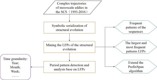
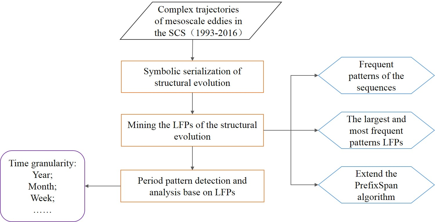
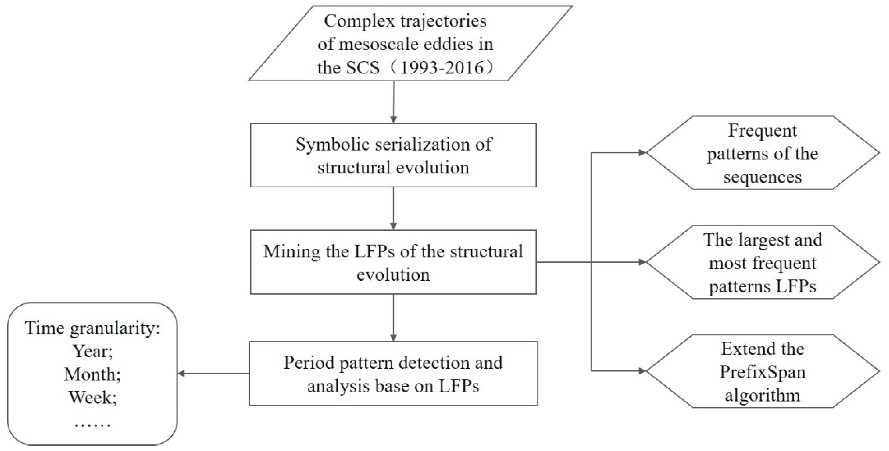
2.2. Mining Periodic Pattern from Complex Trajectories

Figure 2 shows that the proposed PPSE method includes three components. The trajectories were first simplified and represented as a symbol sequence. The PrefixSpan algorithm [10] was expanded and then used to extract the LFPs, from which the yearly, monthly, and weekly periodic patterns were then identified. Each component is illustrated further below.

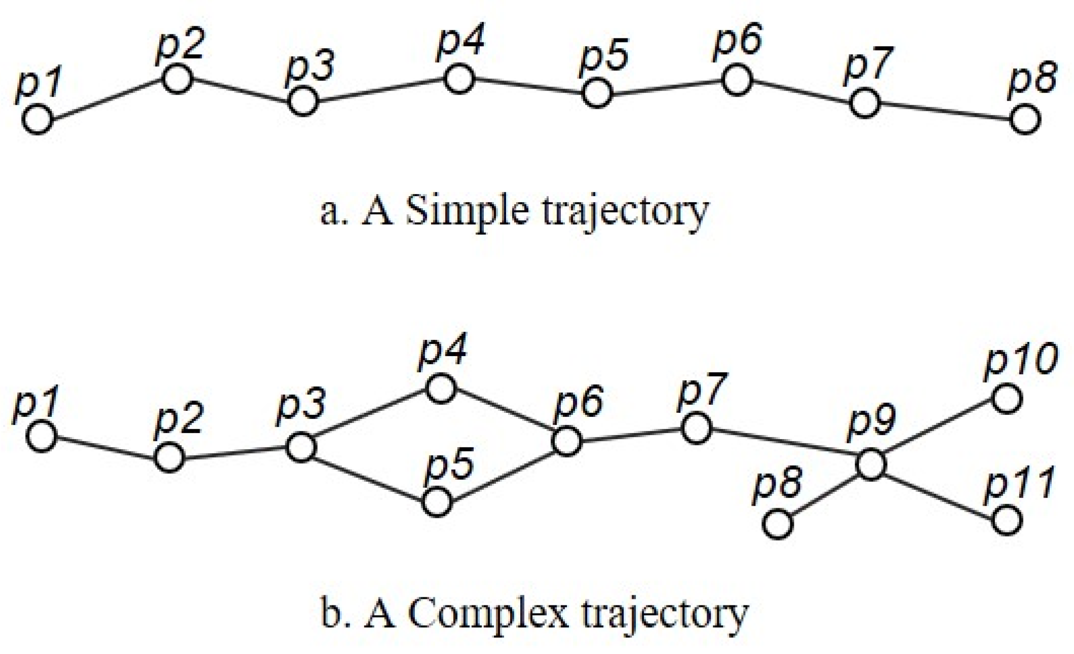
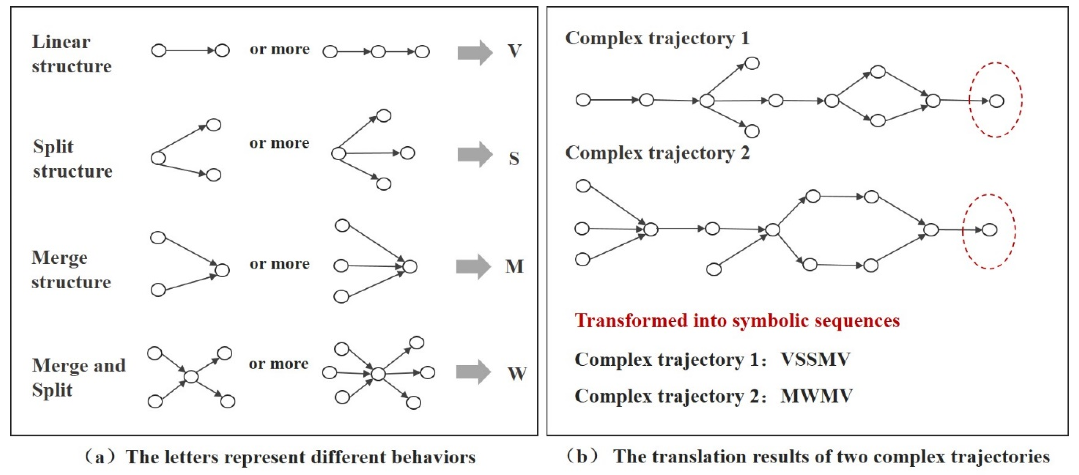
2.2.1. Translation of a Complex Trajectory to a Symbol Sequence

A complex trajectory such as a mesoscale eddy has a linear structure with a different number of branches (Figure 1b). Its complexity could be quantitatively measured by a complexity index η (0 < η ≤ 1), which is the ratio between the number of points along the branch(es) and the points along the whole trajectory. Figure 1b exemplifies a typical complex trajectory, which includes branches formed by both splitting and merging processes. This trajectory has a η of 0.82. The eddy evolves as a whole, as represented from points p1 to p3. After that, it starts to split (p3 splits into p4 and p5 hence p3 is defined as a splitting point). Points p3, p4, and P5 together form a splitting process structure.
Points p4 and p5 then merge into p6, accordingly is defined as a merging point in this study. Points p4, p5, and p6 together form a merging process structure. The eddy then migrates as a whole, as represented by points p6, p7, and p9. Then another eddy (p8) joins p9, which splits into p10 and p11 right away. In this study, a point like p9 is defined as a merging and splitting point as it is simultaneously involved in both merging and splitting processes. Points p7, p8, p9, p10 and p11 form a merging and splitting process structure.
The types of trajectory points (splitting, merging, merging and splitting) mark the structural changes along a complex trajectory. Accordingly, we can translate a complex trajectory into a sequence of symbols, each of which represents an eddy’s specific behavior/stage over its evolution process (Figure 3). Specifically, the letter v was used to represent a linear structure in which all points are not involved in any splitting or merging events. The letter s was used to represent a splitting structure in which an eddy splits into two or even more structures. The letter m was used to represent a merging structure in which two or more eddies merge. Lastly, the letter w was used to represent a structure in which multiple points join together and then split right away.
Depending on the complexity of an eddy trajectory, a sequence of various symbols could be used to illustrate an eddy’s evolution process. For example, the two complex trajectories in Figure 3b could be represented with a sequence of symbols vssmv and mwmv, respectively.
Different priorities would be assigned to the structural changes when they occur in parallel. In this study, higher priority would be given to structure w, then s, then m, and the linear structure v would be given the lowest priority.

2.2.2. The Largest and Most Frequent Pattern (LFP)

A complex trajectory database (CTD) stores multiple trajectory data set CTD:
CTD = { C T R 1 , C T R 2 ,   C T R n }
where CTRi represents the i-th trajectory, which consists of m points.
C T R i = { P 1 , P 2 , ,   P j , , P m }
where Pj represents the jth point along a trajectory. A trajectory point is represented as:
P J = X J , Y J , T J , P t y p e
where Xj and Yj represent its spatial position, Tj the time of motion, and Ptype represents the type of a point which represents an eddy’s specific behavior at Tj over its evolution progress. Ptype could be a(an) starting, ending, splitting, merging, merge–split point, or common point. Any non-starting, ending, splitting, merging, split–merge points are defined as common points in this study.
Once a complex trajectory CTRi is translated into a sequence of symbols, it can be expressed as
C T S i = { P t 1 , P t 2 , , P t k }
where Ptk represents the type of structural change (i.e., those represented with v, s, m, and w in Figure 3a) and the data items in the sequence. The data items are arranged in a chronological order and accordingly the complex trajectories set CTD is translated into a CTS data set, which was stored in the sequence database CTSD.
Definition 1.
The frequent sequence (pattern)
For two complex trajectory structure sequences
A = { P t a 1 , P t a 2 , , P t a n }   and   B = { P t b 1 , P t b 2 , , P t b m }
where n b m   a n d 1 j 1 j 2 j n b m . If P t a 1 P t j 1 , P t a 2 P t j 2 , ,   a n d   P t a n P t j n , A is a subsequence of B and B is the super sequence of A.
The total number of sequence A or B in aCTSDis called the support degree. When it is equal to or greater than a given threshold (usually the minimum support degree (α)), sequence A or B is called the frequent sequence with a length ofan or bm. Frequent sequential pattern mining is essentially utilized to find all subsequence sets with a support degree no less than α in the CTSD. These subsequences are also known as frequent sequential patterns [30].
Definition 2.
The largest and the most frequent sequence pattern LFP
In this study, we first identified the sequences (T) with a length and a support degree over a predefined threshold in the CTSD. From T, we extracted the maximal sequences (L) [30]. The maximal frequent sequences in L with the largest support degree were extracted and stored in S (S = < Pt1, Pt2Pta>). The LFP was defined as the sequence in S with a sequence length LT and the frequency (f), as expressed below:
LFP = S , L T , f
where LT represents the length of the active period of the largest and most frequent sequences S, and f refers to the number of S in the CTSD.

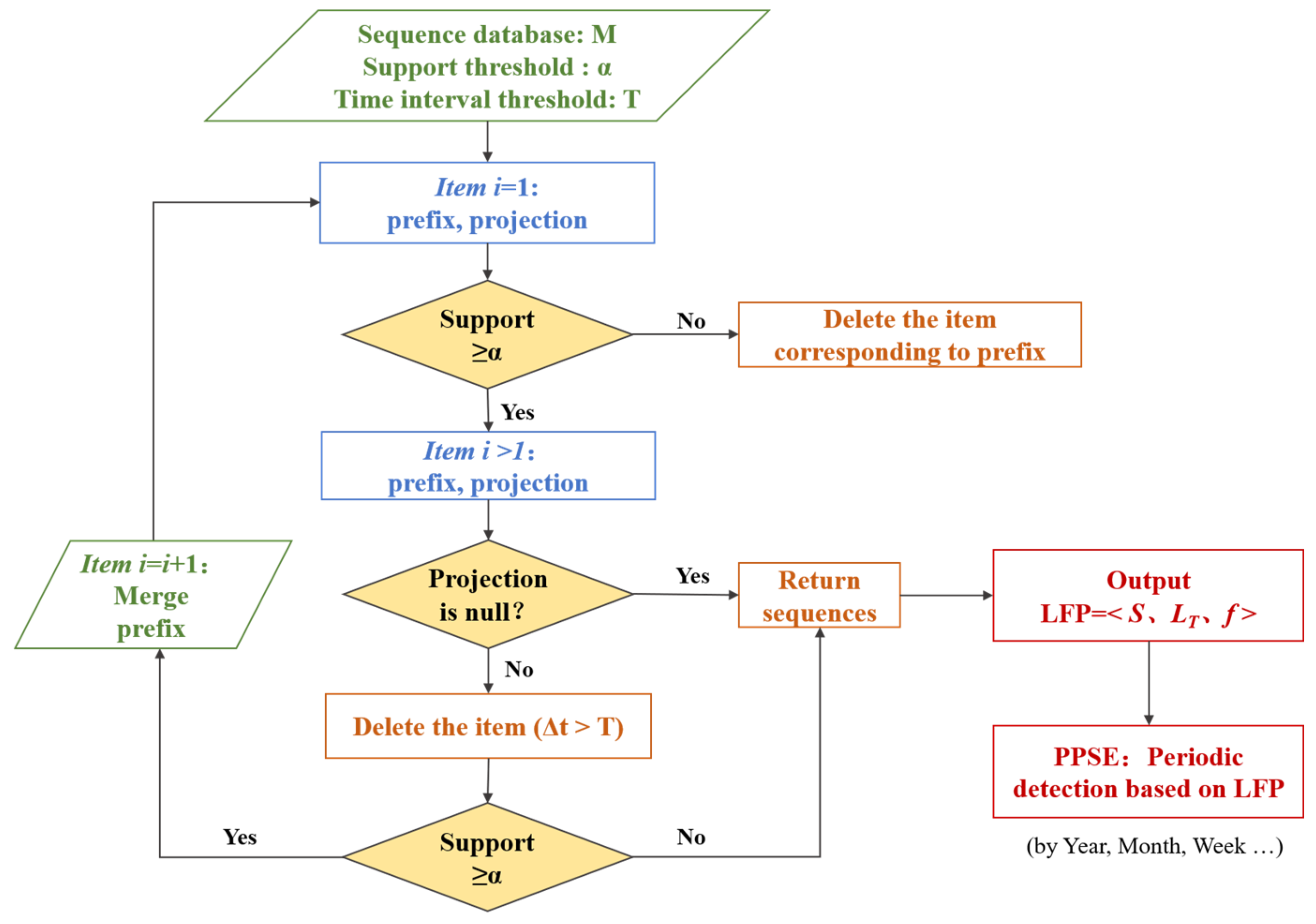
2.2.3. Mining the LFPs Using the PPSE Method

We then used the PPSE method to extract the LFPs. The core idea of the PrefixSpan algorithm is that after each iteration, the subsequent fragments grow until the frequent patterns that meet the minimum support are identified. The algorithm generates a small number of projection libraries, from which the frequent patterns could be more rapidly identified than the Apriori and FP growth algorithms [10]. One of the drawbacks of the PrefixSpan algorithm is that it mainly focuses on the frequency of the sequences and has no consideration of the time change in the events corresponding to the sequence.
Like the PrefixSpan, the PPSE also constructs a projection library of frequent sequences. However, the PPSE sets up a time threshold T and two sequences are paired and compared only when their timing difference is less than the pre-set threshold. The threshold T could be any time granularity. Figure 4 shows how the PPSE was used to identify the LFPs and the major steps are elaborated upon below.
The PrefixSpan algorithm uses two keywords in the predefined step. The first is the prefix, which refers to the subsequence in the front part of the sequence. For instance, when sequences A=<vmvwm> and B= <vmv> are compared, sequence B would be the prefix of sequence A. Furthermore, sequence A could have multiple prefixes such as the sequences consisting of <v>, <vm>, or <vmvw>. The second keyword is the prefix projection, which is also known as suffix. It refers to all non-prefix portions of the sequence. For example, if sequence A =<vmvwm> has a prefix <vmv>, its projection prefix would be <wm>.
In Step 2, a complex trajectory structure sequence set M with n sequences is input to the PPSE. A support degree threshold α and a time threshold T were also set. In step 3, the PPSE constructs a projection library corresponding to prefix and suffix sequences with a length of 1.
Next, the PPSE identifies the prefixes with a length of 1 and counts the total number. If a prefix has a support degree less than the threshold α, the PPSE would delete the item that corresponds to the prefix. The remaining items (i.e., their sequence patterns) would be stored with a length of 1.
The PPSE then recursively identifies the prefixes with a length i and a support degree greater than or equal to the threshold α as shown in the steps below. (1) All projections corresponding to the prefixes are identified. If no projection is found, the PPSE returns the prefixes. (2) The support degree of each subsequence in the projection library is then calculated and the algorithm returns all subsequences with a support degree less than α. (3) The PPSE then deletes the items with a time difference Δt between the time interval of each sub sequence and the average time interval of all sequences greater than T. New prefixes are obtained by combining the single items with the current prefixes. With a new prefix, i = i + 1, the PPSE recursively executes Step (3) until the projection library becomes empty.
All identified frequency patterns are stored in dataset M, from which the LFP was identified as explained in Section 2.2.2. Finally, periodic patterns were found from the LFPs and then analyzed with yearly, monthly, weekly, or daily time granularity. Multiple LFPs, if there are, would be extracted from S.

3. Results

We used the PPSE method to extract LFPs from the ocean eddy clusters in the SCS. A hierarchical clustering method based on a global similarity measuring algorithm for complex trajectories (GSMCT) proposed by Wang et al. [31] was first used to group the complex trajectories of mesoscale eddies in the SCS from January 1993 to December 2016. Figure 5 shows that the AE and CE complex trajectories can be grouped into four clusters, respectively. The numbers of the AE complex trajectories are 84, 385, 44, and 113 in Clusters 1, 2, 3, and 4, respectively. The 730 CE complex trajectories were also grouped into four clusters, with 133, 418, 46, and 133 trajectories in Clusters 1, 2, 3, and 4, respectively.
Spatially, Clusters 1, 2, 3, and 4 are mainly located in the northern SCS, the central SCS, the southeast of Vietnam, and the southern SCS, respectively. The AE and CE complex trajectories in the four abovementioned clusters are then translated into symbol sequences, from which the LFPs are extracted using the PPSE method.
We set two threshold values for the PPSE. The first threshold, the minimum support degree α, is set to 50% or more in this study. According to Pei et al. [10], a pattern with a support degree of over 50% could be deemed as a frequent pattern given that the pattern mining results are affected by a variety of factors. The second threshold, the time interval threshold T, is set to 30 days. Previous researchers such as Chen et al. [28] and Lin et al. [32] have suggested that the number of active days of mesoscale eddies in the SCS is at least 30 and 28 days, respectively.

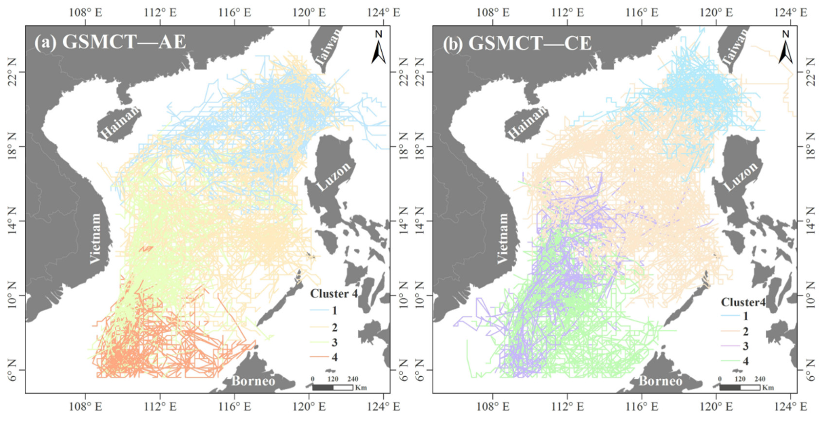
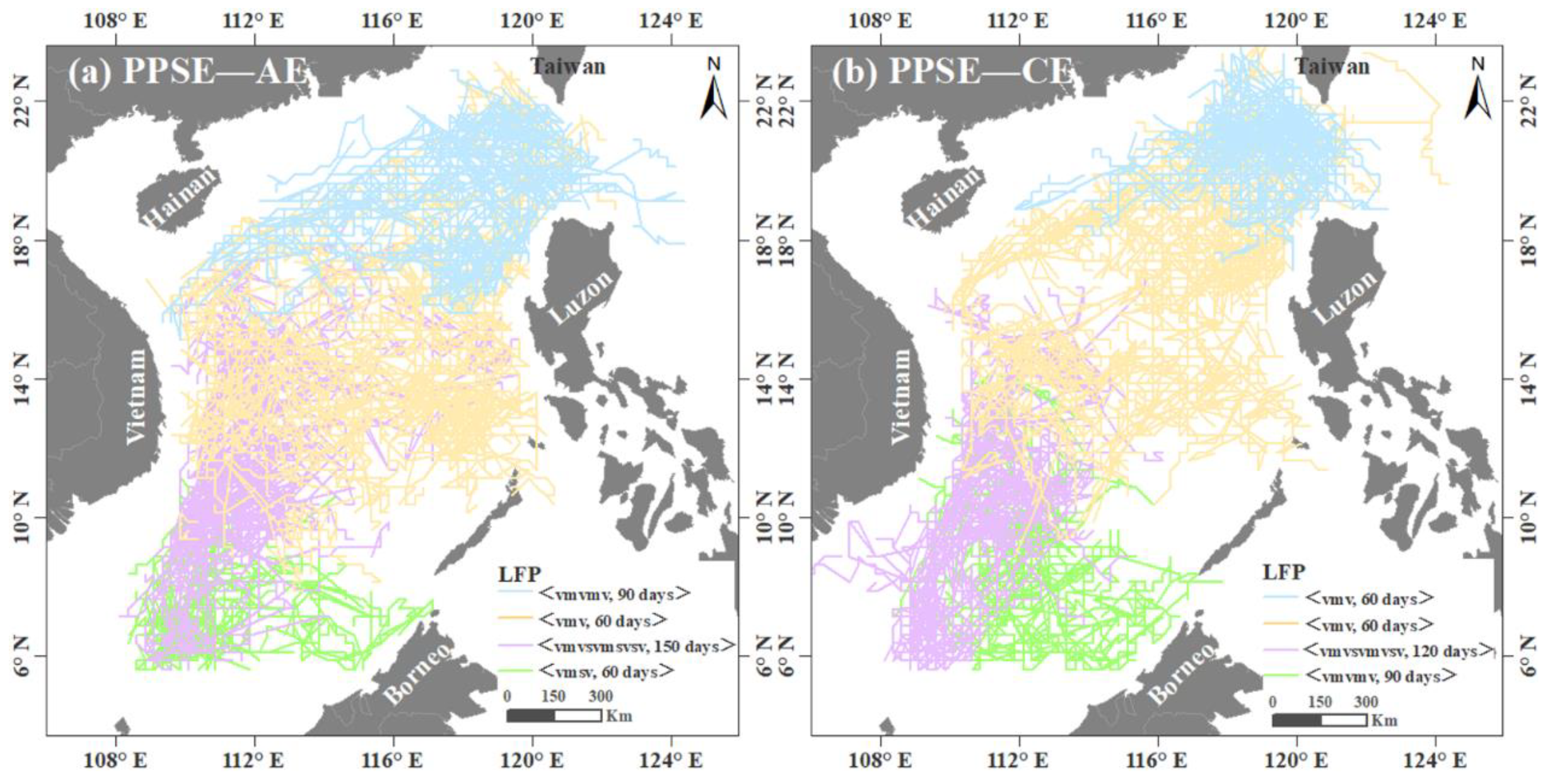
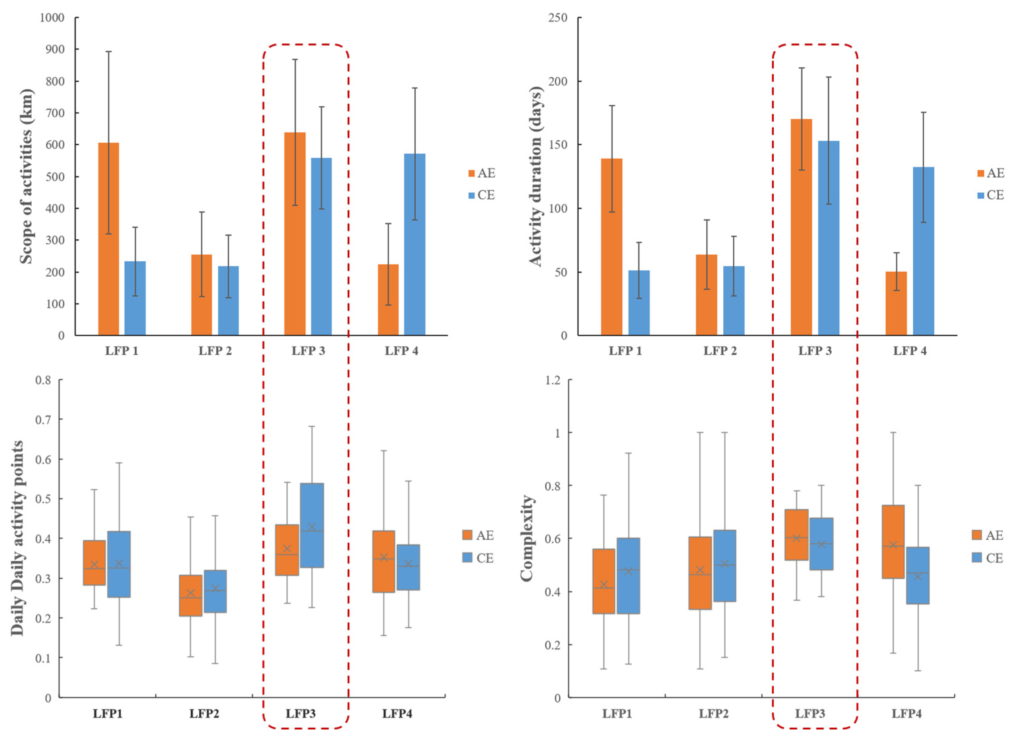
3.1. The LFP Analysis

Table 1 lists the LFPs of the trajectory structures of AE and CE, respectively. Each LFP is represented with its largest and most frequent sequence S, the length of the active cycle LT for the sequence S, the number of trajectories, as well as the percentage of trajectories. The percentage is calculated as the proportion of the trajectories in the sequence S in relation to the total number of trajectories within that specific cluster.
Very similar LFPs were found for the four AE(a) and CE(b) clusters (Figure 6). On average, more than 60% of the complex AE and CE trajectories are dominated by the merge structural change in the northern (orange trajectories), the central (blue trajectories) and the southern (green trajectories) SCS. These LFPs (LFP 1, LFP 2, LFP 3) have a 60- or 90-day activity period of structural changes.
In contrast, the LFP3 of AE and CE in the southeast of Vietnam have a much longer active period of 150 days and 120 days, respectively. Furthermore, the LFP3 also shows a more complex structure formed by the constantly merging and splitting behaviors of the eddies. It is also interesting to note that the LFP3 of AE is very similar to the LFP3 of CE, with a similarity indicator of 90%. Specifically, the AE LFP 3 has a structure of <vmvsvmsvsvsv>, whereas the CE LFP 3 structure is <vmvsvmvsv>, i.e., the AE has only one more splitting behavior than the CE.
Figure 7 shows the statistical analysis results of the AE and CE LFPs regarding their scope of activities (the maximum distance between any two points along a specific trajectory), active period (the lifespan of the trajectory), number of daily active points (the number of different positions that an eddy may occupy per day), and trajectory complexity. LFP 3 in the southeast of Vietnam is significantly different from the other LFPs as it has the widest moving range (AE is 638.72km, CE is 559.25km), the longest active period (AE is 170 days, CE is 153 days), the highest number of active points per day (AE is 0.38, CE is 0.43), and the highest complexity (AE is 0.61, CE is 0.59) in the SCS.

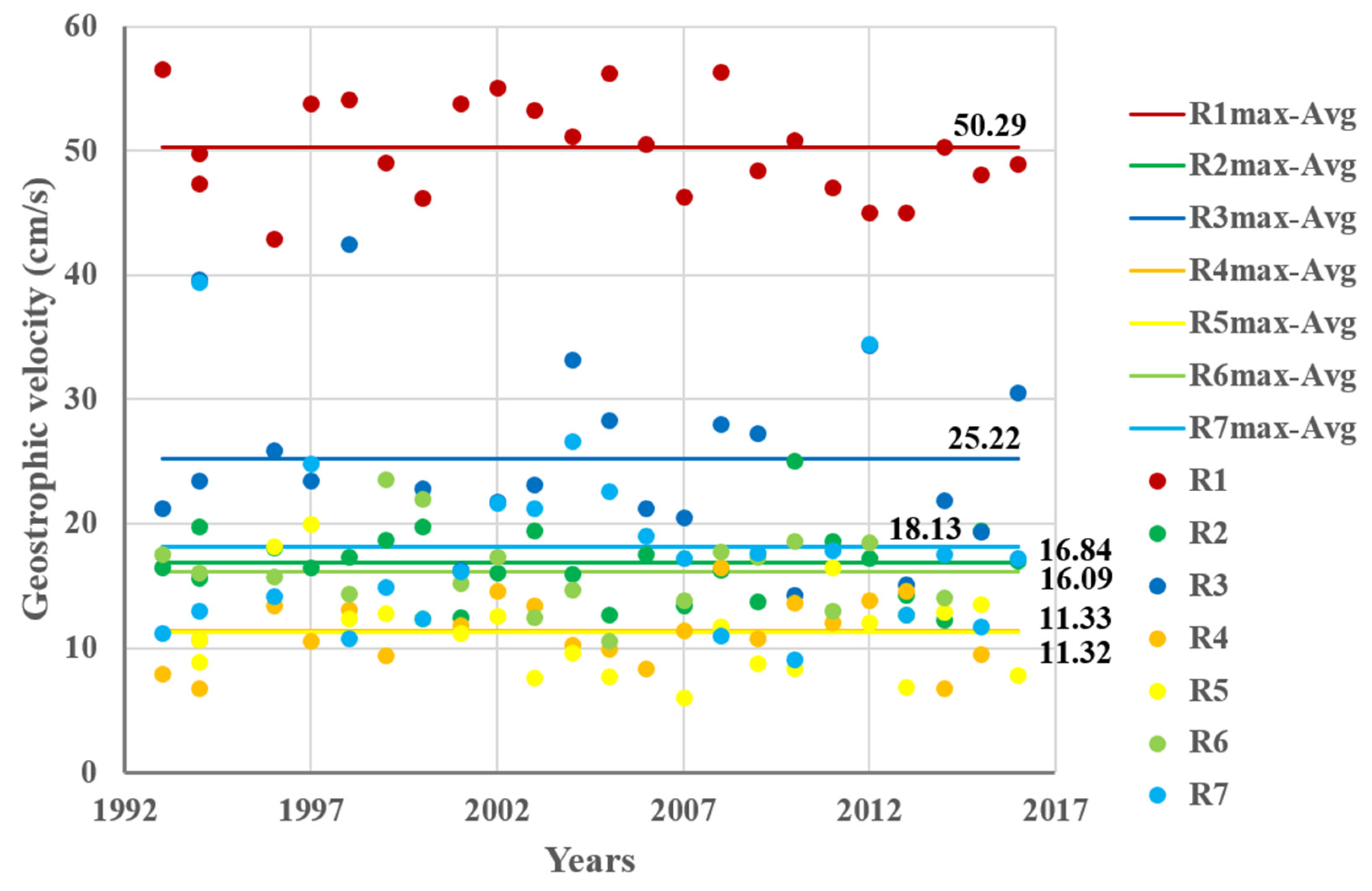
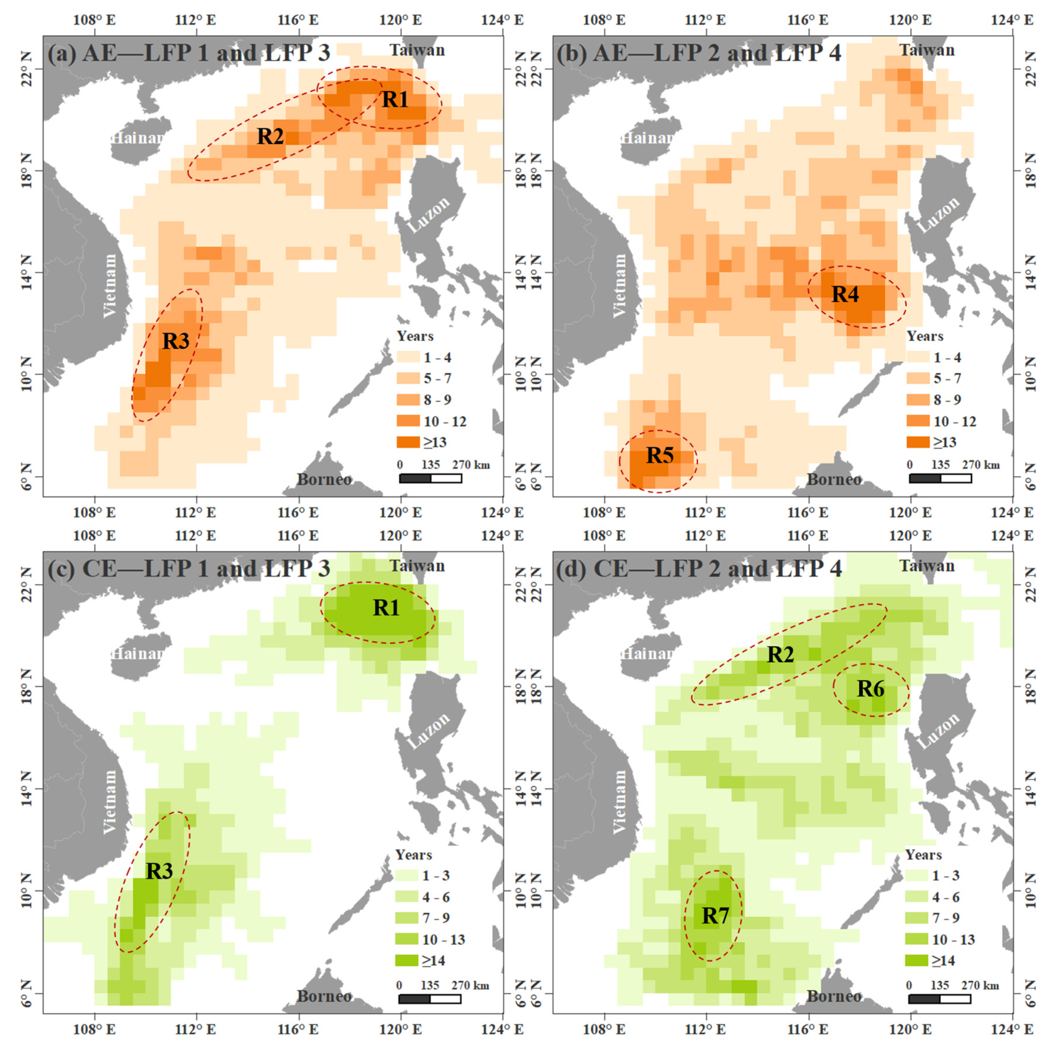
3.2. Periodic Pattern Discovery

Figure 8 shows the interannual migration channels of AE and CE LFPs per 0.5° × 0.5° (about 55km x 55km), which is close to the migration range of eddies in the SCS [28]. The number of years per grid refers to the different years when the trajectories appear in that grid. The oval regions represent the migration channels (R1-R7) that are close to the LFPs with significant interannual periodic pattern (17–24 years, accounting for 70–100% of the 24 years). Table 2 shows the statistical characteristics of these channels.
The seven migration channels close to the AE and CE LFPs are located in the southwest of Taiwan Island (R1), the northern shelf slope of SCS (R2), the southeast of Vietnam (R3), the southwest and northwest of Luzon Island (R4, R6), and the southernmost part of the SCS (R5, R7). Along these migration channels, the LFPs show an annual periodic pattern (Table 2).
Previous studies have shown that R2 is a typical eddy migration channel and the other migration channels (R1, R3-R6) are the major places where most eddies emerge [28,32,33]. The consistency between the previous results and this study regarding the migration channels confirms the PPSE is effective in identifying the LFPs from complex trajectories of mesoscale ocean eddies in the SCS.

4. Discussion

The LFPs identified in this study provide new insights regarding the evolution of the mesoscale ocean eddies in the SCS. The most structurally complicated LFP is found in the southeast of Vietnam, suggesting that the eddies in this region show more complicated evolution behaviors. The AE and CE LFPs in the southeast of Vietnam are very similar and both have the longest active cycle, the widest range of activities, the highest complexity, and are the most active among all LFPs found in the SCS.
The singular characteristics of the LFPs in the southeast of Vietnam show that the ocean eddies in this region are quite different from those in other regions in the SCS. Previous studies mainly attribute the emergence of eddies in the southeast of Vietnam to the offshore flow driven by the southwest monsoon [34]. Water vorticity energy in this region is also high [35]. The strong interaction between the offshore flow and the high vorticity energy in this region may force eddies to split and merge more frequently. Accordingly, a more structurally complicated LFP could be found with a longer active cycle and a wider range of activities.
The AE and CE LFPs in the migration channels show a cycle ranging from 17 to 24 years in the southwest of Taiwan Island (R1), northern shelf slope of SCS (R2), the southeast of Vietnam (R3, R5, R7), the southwest and northwest of Luzon Island (R4, R6), respectively. These migration channels are basically consistent with what previous studies have shown and different driving forces have been cited to explain these migration channels. For example, the frequent generation and movement of eddies in Channel R1 are mainly attributed to the black tide invasion [28], the baroclinic instability of the background currents [28] and the change in local wind stress [36]. The topography in the northern slope of the SCS drives eddies to migrate westward through Channel R2 [33]. Channels R3, R5 and R7 in the southeast of Vietnam are formed by the easterly jet flow [28,37], whereas Channels R4, R6 in southwest and northwest of Luzon are attributed to the strong wind stress curl caused by the interaction of wind and topography [36,37].
The geostrophic flow velocity is also frequently used to study the generation of a mesoscale ocean eddy and it is defined as:
V = u g 2 + v g 2
where u g and v g is the zonal and meridional geostrophic currents, respectively.
The 1993 to 2006 flow field data from the AVISO (Figure 9) show that the maximum yearly average flow velocity within channel R1 is 50.29 cm/s. The maximum yearly average flow velocity in the other channels (R2-R7) ranges from 11.32 to 25.2 cm/s, which is higher than that reported in a previous study (10 cm/s) [28]. The larger flow velocity within a migration channel could be associated with a stronger shear force, which may cause the eddies to split and merge more.

5. Conclusions

We proposed a method to identify the LFPs from the AE and CE complex trajectories of mesoscale eddies in the SCS. We first grouped the eddies into different clusters, from which the LFP was identified. Our results show that the LFP in the southeast of Vietnam is the most complicated and the most active one among all LFPs in the SCS. In the southeast of Vietnam, the AE and CE LFPs share over a 90% similarity and both have the longest period of activity and the widest range of activity. The LFPs show a cycle ranging from 17 to 24 years. Additionally, the LFPs revealed seven eddy migration channels, within which the maximum yearly average current velocity is over 11 cm/s. The high shear forces associated with the faster currents within the channels may cause more eddy generation, spitting, and merging activities.
This study reveals the migration patterns of the mesoscale ocean eddies in the SCS from the perspective of their trajectory structures and adds new knowledge to the field. However, the PPSE could be improved by coupling the time dimension, space dimension, and structure relationship more tightly, which is on the agenda for our future studies.

Author Contributions

Conceptualization, Huimeng Wang and Yunyan Du; methodology, Huimeng Wang; software, Nan Wang; validation, Huimeng Wang, Yunyan Du and Fuyuan Liang; formal analysis, Nan Wang; investigation, Huimeng Wang; resources, Jiawei Yi; data curation, Jiawei Yi; writing—original draft preparation, Huimeng Wang; writing—review and editing, Fuyuan Liang; visualization, Huimeng Wang; supervision, Yunyan Du; project administration, Yunyan Du; funding acquisition, Yunyan Du. All authors have read and agreed to the published version of the manuscript.

Funding

This work was supported in part by a grant from the National Science Foundation of China (41671445).

Conflicts of Interest

The authors declare no conflict of interest.

References

  1. Mamoulis, N.; Cao, H.; Kollios, G. Mining, Indexing, and Querying Historical Spatiotemporal Data. In Proceedings of the Tenth ACM SIGKDD International Conference on Knowledge Discovery and Data Mining, Seattle, WA, USA, 25–25 August 2004; pp. 236–245. [Google Scholar]
  2. Cao, H.; Mamoulis, N.; Cheung, D.W. Discovery of Periodic Patterns in Spatiotemporal Sequences. IEEE Trans. Knowl. Data Eng. 2007, 19, 453–467. [Google Scholar] [CrossRef] [Green Version]
  3. Jindal, T.; Giridhar, P.; Tang, L.A. Spatiotemporal Periodical Pattern Mining in Traffic Data. In Proceedings of the 2nd ACM SIGKDD International Workshop on Urban Computing, Chicago, IL, USA, 11–14 August 2013. [Google Scholar]
  4. Zhang, D.; Lee, K.; Lee, I. Semantic periodic pattern mining from spatio-temporal trajectories. Inf. Sci. 2019, 502, 164–189. [Google Scholar] [CrossRef]
  5. Nan, F.; He, Z.; Zhou, H.; Wang, N. Three long-lived anticyclonic eddies in the northern South China Sea. J. Geophys. Res. Space Phys. 2011, 116. [Google Scholar] [CrossRef]
  6. Yi, J.; Du, Y.; Liang, F.; Zhou, C.; Wu, D.; Mo, Y. A representation framework for studying spatiotemporal changes and interactions of dynamic geographic phenomena. Int. J. Geogr. Inf. Sci. 2014, 28, 1010–1027. [Google Scholar] [CrossRef]
  7. Wang, H.; Du, Y.; Yi, J.; Sun, Y.; Liang, F. A New Method for Measuring Topological Structure Similarity between Complex Trajectories. IEEE Trans. Knowl. Data Eng. 2019, 31, 1836–1848. [Google Scholar] [CrossRef]
  8. Agrawal, R.; Srikant, R. Mining Sequential Patterns. In Proceedings of the Eleventh International Conference on Data Engineering, Taipei, Taiwan, 6–10 March 1995. [Google Scholar]
  9. Han, J.W.; Gong, W.; Yin, Y.W. Mining Segment-Wise Periodic Patterns in Time-Related Databases. In Proceedings of the 4th International Conference on Knowledge Discovery and Data Mining, New York, NY, USA, 27 August 1998. [Google Scholar]
  10. Pei, J.; Han, J.; Mortazavi-Asl, B.; Wang, J.; Pinto, H.; Chen, Q.; Dayal, U.; Hsu, M.-C. Mining sequential patterns by pattern-growth: The PrefixSpan approach. IEEE Trans. Knowl. Data Eng. 2004, 16, 1424–1440. [Google Scholar] [CrossRef] [Green Version]
  11. Nurulhaq, N.Z.; Sitanggang, I.S. Sequential Pattern Mining on hotspot data in Riau province using the PrefixSpan algorithm. In Proceedings of the International Conference on Adaptive & Intelligent Agroindustry, Bogor, Indonesia, 3–4 August 2015. [Google Scholar]
  12. Yang, K.-J.; Hong, T.-P.; Chen, Y.-M.; Lan, G.-C. Projection-based partial periodic pattern mining for event sequences. Expert Syst. Appl. 2013, 40, 4232–4240. [Google Scholar] [CrossRef]
  13. He, Z.; Wang, X.S.; Lee, B.S.; Ling, A.C.H. Mining partial periodic correlations in time series. Knowl. Inf. Syst. 2006, 15, 31–54. [Google Scholar] [CrossRef]
  14. Yuan, G.; Zhao, J.; Xia, S.; Zhang, Y.; Li, W. Multi-granularity periodic activity discovery for moving objects. Int. J. Geogr. Inf. Sci. 2016, 31, 435–462. [Google Scholar] [CrossRef]
  15. Ying, J.J.-C.; Lee, W.-C.; Tseng, V.S. Mining geographic-temporal-semantic patterns in trajectories for location prediction. ACM Trans. Intell. Syst. Technol. 2013, 5, 1–33. [Google Scholar] [CrossRef]
  16. Cui, W.; Wang, W.; Zhang, J.; Yang, J. Multicore structures and the splitting and merging of eddies in global oceans from satellite altimeter data. Ocean Sci. 2019, 15, 413–430. [Google Scholar] [CrossRef] [Green Version]
  17. Zhang, Z.; Wang, W.; Qiu, B. Oceanic mass transport by mesoscale eddies. Science 2014, 345, 322–324. [Google Scholar] [CrossRef] [PubMed]
  18. Rodríguez-Marroyo, R.; Viúdez, Á; Ruiz, S. Vortex Merger in Oceanic Tripoles. J. Phys. Oceanogr. 2011, 41, 1239–1251. [Google Scholar] [CrossRef] [Green Version]
  19. Li, Q.-Y.; Sun, L.; Lin, S.-F. GEM: A dynamic tracking model for mesoscale eddies in the ocean. Ocean Sci. 2016, 12, 1249–1267. [Google Scholar] [CrossRef] [Green Version]
  20. Yi, J.; Du, Y.; He, Z.; Zhou, C. Enhancing the accuracy of automatic eddy detection and the capability of recognizing the multi-core structures from maps of sea level anomaly. Ocean Sci. 2014, 10, 39–48. [Google Scholar] [CrossRef] [Green Version]
  21. Yi, J.; Du, Y.; Liang, F.; Zhou, C. An auto-tracking algorithm for mesoscale eddies using global nearest neighbor filter. Limnol. Oceanogr. Methods 2017, 15, 276–290. [Google Scholar] [CrossRef]
  22. Pujol, M.; Faugère, Y.; Taburet, G.; Dupuy, S.; Pelloquin, C.; Ablain, M.; Picot, N. DUACS DT2014: The new multi-mission altimeter data set reprocessed over 20 years. Ocean Sci. 2016, 12, 1067–1090. [Google Scholar] [CrossRef] [Green Version]
  23. Okubo, A. Horizontal dispersion of floatable particles in the vicinity of velocity singularities such as convergences. Deep Sea Res. Oceanogr. Abstr. 1970, 17, 445–454. [Google Scholar] [CrossRef]
  24. Weiss, J. The dynamics of enstrophy transfer in two-dimensional hydrodynamics. Phys. D Nonlinear Phenom. 1991, 48, 273–294. [Google Scholar] [CrossRef]
  25. Chelton, D.B.; Schlax, M.G.; Samelson, R.M. Global observations of nonlinear mesoscale eddies. Progr. Oceanogr. 2011, 91, 167–216. [Google Scholar] [CrossRef]
  26. Morrow, R.; Birol, F.; Griffin, D.; Sudre, J. Divergent pathways of cyclonic and anti-cyclonic ocean eddies. Geophys. Res. Lett. 2004, 31, 24311. [Google Scholar] [CrossRef]
  27. Henson, S.; Thomas, A.C. A census of oceanic anticyclonic eddies in the Gulf of Alaska. Deep Sea Res. Part I Oceanogr. Res. Pap. 2008, 55, 163–176. [Google Scholar] [CrossRef]
  28. Chen, G.; Hou, Y.; Chu, X. Mesoscale eddies in the South China Sea: Mean properties, spatiotemporal variability, and impact on thermohaline structure. J. Geophys. Res. Space Phys. 2011, 116, 1–20. [Google Scholar] [CrossRef]
  29. Sudre, J.; Maes, C.; Garçon, V. On the global estimates of geostrophic and Ekman surface currents. Limnol. Oceanogr. Fluids Environ. 2013, 3, 1–20. [Google Scholar] [CrossRef] [Green Version]
  30. Luo, C.; Chung, S.M. A scalable algorithm for mining maximal frequent sequences using a sample. Knowl. Inf. Syst. 2007, 15, 149–179. [Google Scholar] [CrossRef]
  31. Wang, H.; Du, Y.; Sun, Y.; Liang, F.; Yi, J.; Wang, N. Clustering Complex Trajectories Based on Topologic Similarity and Spatial Proximity: A Case Study of the Mesoscale Ocean Eddies in the South China Sea. ISPRS Int. J. Geo-Inf. 2019, 8, 574. [Google Scholar] [CrossRef] [Green Version]
  32. Lin, P.F.; Fan, W.; Chen, Y.L. Temporal and spatial variation characteristics on eddies in the South China Sea I. Statistical analyses. Acta Oceanol. Sin. 2008, 29, 14–22. [Google Scholar]
  33. Nan, F.; Xue, H.; Yu, F. Kuroshio intrusion into the South China Sea: A review. Prog. Oceanogr. 2015, 137, 314–333. [Google Scholar] [CrossRef] [Green Version]
  34. Chen, G.; Hou, Y.; Zhang, Q.; Chu, X. The eddy pair off eastern Vietnam: Interannual variability and impact on thermohaline structure. Cont. Shelf Res. 2010, 30, 715–723. [Google Scholar] [CrossRef]
  35. Yang, H.; Wu, L.; Liu, H.; Yu, Y. Eddy energy sources and sinks in the South China Sea. J. Geophys. Res. Oceans 2013, 118, 4716–4726. [Google Scholar] [CrossRef]
  36. Wang, G. Mesoscale eddies in the South China Sea observed with altimeter data. Geophys. Res. Lett. 2003, 30, 2121. [Google Scholar] [CrossRef] [Green Version]
  37. Gan, J.; Qu, T. Coastal jet separation and associated flow variability in the southwest South China Sea. Deep Sea Res. Part. I Oceanogr. Res. Pap. 2008, 55, 1–19. [Google Scholar] [CrossRef]
Figure 1. (a) A simple trajectory and (b) a complex trajectory.
Ijgi 09 00441 g001
Figure 2. A flow chart showing the major components of the periodic pattern mining of structural evolution (PPSE) method.
Ijgi 09 00441 g002
Figure 3. The letters represent different behaviors of an eddy (a) and the translation results (sequence of symbols) of two complex trajectories (b).
Ijgi 09 00441 g003
Figure 4. A flow chart showing how the PPSE works.
Ijgi 09 00441 g004
Figure 5. Clustering results of complex trajectories of anticyclonic eddies (AE) (a) and cyclonic eddies (CE) (b) in the South China Sea (SCS) using the global similarity measuring algorithm for complex trajectories (GSMCT) proposed by Wang et al. [31].
Ijgi 09 00441 g005
Figure 6. The LFPs for the structural evolution of AE (a) and CE (b) in the SCS based on the PPSE algorithm.
Ijgi 09 00441 g006
Figure 7. Statistical characteristics of the AE and CE LFPs.
Ijgi 09 00441 g007
Figure 8. The migration channels as revealed by the AE and CE complex trajectory LFPs.
Ijgi 09 00441 g008
Figure 9. The maximum (represented with circles) and annual average velocity (represented with lines) of the currents in the migration channels (R1-R7).
Ijgi 09 00441 g009
Table 1. The largest and most frequent patterns (LFPs) of the trajectory structures of AE and CE in the SCS.
Space area
(Pattern)
AECE
Northern cluster:
LFP 1
<vmvmv, 90, 52(62%)><vmv, 60, 84(63%)>
Central cluster:
LFP 2
<vmv, 60, 228(59%)><vmv, 60, 250(60%)>
Southeast of Vietnam:
LFP 3
<vmvsvmsvsv, 150, 33(75%)><vmvsvmvsv, 120, 26(57%)>
Southern cluster:
LFP 4
<vmsv, 60, 70(55%)><vmvmv, 90, 78(59%)>
Table 2. The AE and CE LFPs show an annual periodic pattern LFPs in the seven migration channels.
LFPAE
Mobile channel R: cycle years
CE
Mobile channel R: cycle years
LFP 1R1 (21 years): 1993, 1994, 1995, 1996, 1997, 1998, 1999, 2000, 2001, 2002, 2003, 2004, 2005, 2006, 2007, 2008, 2011, 2012, 2013, 2015, 2016
R2 (20 years): 1993, 1995, 1996, 1997, 1998, 1999, 2000, 2001, 2002, 2003, 2005, 2006, 2007, 2008, 2011, 2012, 2013, 2014, 2015, 2016
R1 (23 years): 1993, 1994, 1995, 1996, 1997, 1998, 1999, 2000, 2001, 2002, 2003, 2004, 2005, 2006, 2007, 2009, 2010, 2011, 2012, 2013, 2014, 2015, 2016
LFP 2R4 (22 years): 1993, 1994, 1995, 1996, 1997, 1998, 1999, 2001, 2002, 2003, 2004, 2005, 2006, 2007, 2008, 2009, 2010, 2011, 2012, 2013, 2014, 2015,R2 (20 years): 1993, 1994, 1995, 1997, 1998, 1999, 2000, 2001, 2002, 2003, 2004, 2005, 2007, 2008, 2009, 2010, 2011, 2012, 2013, 2016
R6 (19 years): 1993, 1994, 1996, 1998, 1999, 2000, 2001, 2002, 2003, 2004, 2005, 2007, 2008, 2009, 2010, 2011, 2012, 2013, 2014,
LFP 3R3 (17 years): 1994, 1995, 1996, 1997, 1998, 2000, 2001, 2004, 2005, 2007, 2008, 2009, 2012, 2013, 2014, 2015, 2016R3 (17 years): 1993, 1994, 1995, 1996, 1997, 2000, 2001, 2002, 2003, 2006, 2008, 2009, 2010, 2012, 2013, 2014, 2016
LFP 4R5 (22 years): 1994, 1995, 1996, 1997, 1998, 1999, 2000, 2001, 2002, 2003, 2004, 2005, 2007, 2008, 2009, 2010, 2011, 2012, 2013, 2014, 2015, 2016R7 (24 years): 1993, 1994, 1995, 1996, 1997, 1998, 1999, 2000, 2001, 2002, 2003, 2004, 2005, 2006, 2007, 2008, 2009, 2010, 2011, 2012, 2013, 2014, 2015, 2016

