LASDU: A Large-Scale Aerial LiDAR Dataset for Semantic Labeling in Dense Urban Areas

Abstract

The semantic labeling of the urban area is an essential but challenging task for a wide variety of applications such as mapping, navigation, and monitoring. The rapid advance in Light Detection and Ranging (LiDAR) systems provides this task with a possible solution using 3D point clouds, which are accessible, affordable, accurate, and applicable. Among all types of platforms, the airborne platform with LiDAR can serve as an efficient and effective tool for large-scale 3D mapping in the urban area. Against this background, a large number of algorithms and methods have been developed to fully explore the potential of 3D point clouds. However, the creation of publicly accessible large-scale annotated datasets, which are critical for assessing the performance of the developed algorithms and methods, is still at an early age. In this work, we present a large-scale aerial LiDAR point cloud dataset acquired in a highly-dense and complex urban area for the evaluation of semantic labeling methods. This dataset covers an urban area with highly-dense buildings of approximately 1 km² and includes more than three million points with five classes of objects labeled. Moreover, experiments are carried out with the results from several baseline methods, demonstrating the feasibility and capability of the dataset serving as a benchmark for assessing semantic labeling methods.

1. Introduction

The semantic labeling of urban areas is an essential but challenging task for a wide variety of applications such as city mapping, outdoor navigation, and traffic monitoring. The rapid advance of Light Detection and Ranging (LiDAR) systems has aided in the solution of this task, leading towards an accessible, affordable, accurate, and applicable stage with the use of 3D point clouds. Among all types of LiDAR systems using various platforms, the airborne one (i.e., airborne laser scanning (ALS) has already been proven to be a versatile technique for large-scale, high-resolution, and highly-accurate topographic data acquisition, providing direct measurements of the ground elevation [1]. Although researchers and engineers have been aware of the potential of airborne laser scanning (ALS) data and have tried to utilize it in various tasks, there is a challenge prior to any application using ALS data: we have to interpret semantic information of observed scenes presented by 3D point clouds of ALS. The primary objective of the semantic interpretation of ALS point clouds is to assign each 3D point with a unique semantic label indicating the class of specific objects in the scene, in accordance with geometric or radiometric information provided by the point itself and the points in its neighborhood.

To achieve the semantic labeling of points, a large number of algorithms and methods have been developed to solve puzzles hidden in the measured 3D point clouds. For many applications and studies, the performance of the developed algorithm or method should be assessed through public standard benchmark datasets, which contributes significantly to algorithm development, evaluation, and comparison [2]. For the semantic labeling of ALS point clouds, we also naturally need standard frameworks for conducting the evaluation process, which should be assisted by benchmark datasets. However, the creation of publicly accessible large-scale annotated datasets, which are critical for assessing the performance of developed algorithms and methods, is still at an early age. To this end, in this paper, a new large-scale annotated aerial point cloud dataset acquired in a highly-dense urban area is presented. This dataset covers an urban area with highly-dense buildings of approximately 1 km² and includes more than 3 million points with five classes of objects labeled. An example of a small area of the presented dataset is shown in Figure 1.

The objective of this paper is to introduce a new annotated ALS dataset serving as the benchmark for evaluating the methods and algorithms of point cloud semantic labeling. In addition, by conducting experiments using several reference methods, we aim to determine the potential influence of the use of hierarchical and multi-scale strategies in deep learning-based methods. Thus, the main contribution of this paper is two-fold: one is the presentation of a large-scale annotated ALS point cloud dataset with point-wise labels for semantic labeling. The data were acquired in a challenging highly-dense urban area, with multiple types of complex buildings, infrastructures, and vegetation measured and annotated. With similar characteristics but more challenging scenarios and larger size, this dataset is significantly complementary for the commonly used ISPRS 3D semantic labeling dataset. The other contribution of this paper is the evaluation and analysis of semantic labeling performance on the proposed dataset using several deep learning-based methods considering various scale strategies. From evaluation results, we confirmed that the scale factors have a significant impact on the performance of the deep neural network for point cloud semantic labeling in a scenario in which objects have various geometric sizes.

2. Benchmark Datasets from LiDAR Point Clouds

In the last decade, a wide range of benchmark datasets for various point cloud processing tasks has been presented. For example, there are exterminating benchmark datasets for point cloud registration such as the Real-World Scans with Small Overlap (RESSO) dataset [3] and the large-scale terrestrial LiDAR scanning (TLS) point cloud registration benchmark dataset (WHU-TLS) [4,5]. With respect to semantic segmentation and semantic labeling, there are already plentiful benchmark datasets that have been presented, such as the Oakland outdoor mobile LiDAR scanning (MLS) dataset [6], ISPRS Semantic labeling benchmark [7], Semantic3D.net TLS dataset (Semantic3D) [8], MLS1-TUM City Campus (2016) dataset [9], Paris–Lille-3D MLS dataset [10], TorontoCity dataset [11], and Toronto-3D MLS dataset [12]. In particular, the TorontoCity dataset includes data from sources of aerial RGB images, streetview panoramas, street-view LIDAR, and airborne LIDAR, covering the entire greater Toronto area. Instead of manually annotated labels, various high-precision maps were utilized to create ground truth, which made this dataset a powerful tool for the evaluation of developed methods in a wide variety of applications. However, for any of the benchmark point cloud datasets, there is always a delimitation for the platform used for measuring the 3D points. This is because the attributes, accuracy, density, and quality of different types of point clouds vary significantly due to the different platforms used in the measurement [13]. Thus, to evaluate algorithms and methods designed for different applications, different types of point clouds (i.e., point clouds acquired from different types of platforms) used for generating a benchmark dataset should be considered. Moreover, the costs and difficulties of generating these benchmark datasets are also completely different. In the following subsections, we will give a brief review of the differences in characteristics between LiDAR point clouds acquired with various platforms and give an introduction to representative ALS point cloud datasets for 3D semantic labeling.

The remainder of this paper is organized as follows. In Section 2, a brief review of exiting benchmark ALS datasets for semantic labeling is given. In Section 3, the basic information and features, as well as the challenges, of the presented LASDU dataset are elaborated. Section 4 introduces conducted experiments using the presented dataset. Section 5 reports the experimental results and gives a detailed discussion and analysis of the performance. Finally, Section 6 concludes the paper and offers future work.

2.1. Differences between LiDAR Point Clouds Acquired with Various Platforms

As mentioned above, with different LiDAR systems and platforms, the benchmark datasets generated with different point clouds will reveal various characteristics. For instance, the point density can vary from less than 10 points per m² (pts/m²) to 5000 pts/m² [2]. Generally, according to the platforms used in the measuring campaign, point clouds acquired with LiDAR systems are categorized into major types: TLS point clouds, MLS point clouds, and ALS point clouds.

TLS works with a static platform which is usually mounted on a tripod with accurate and stable scanner positions. TLS can provide middle and close-range measurements, and the point densities vary along with the measuring distances [14]. Thus, TLS can be applied to acquire point clouds with high accuracy in applications such as indoor mapping [15], archaeology [16], and the monitoring [17] of buildings and man-made infrastructures. However, due to the static working platform, the field of view for TLS is always restricted due to occlusions. This is an especially severe problem in the measurement of urban scenarios with crowded and high-rise buildings.

MLS commonly works on a mobile platform (e.g., cars or boats). Compared with TLS, the laser scan from MLS provides a side-looking view of the building facades and streets or river banks, which makes it a useful tool for tasks such as 3D city mapping [18] and autonomous driving [6]. Moreover, benefiting from a flexible and moving platform, point clouds from MLS can, to some extent, avoid the occlusion phenomena occurring in the data acquired via TLS. ALS works on aircraft or UAVs, and the scanning is conducted during the flight. Measurements with ALS can cover a large area, but the point density relies on the scanning frequency and flight altitude. Based on this characteristic, ALS is frequently utilized in urban mapping [7], agriculture investigation, and forestry surveying [19]. However, in its early stage of development, ALS can only provide 2.5D point clouds, the characteristics of which are closer to DEM or depth image data. The laser scanning conducted via a UAV platform can also be categorized into the ALS. Thanks to the smaller size and lighter weight of its platform, UAV-based ALS can offer a high operational flexibility [2], which can even be used in an indoor scenario [20]. One major disadvantage of ALS is the instability of the working platform, meaning that the point clouds acquired by ALS normally have a relatively low geo-positioning accuracy; in some situations, motion compensation is also required for the data processing.

2.2. Representative ALS Point Cloud Datasets for 3D Semantic Labeling

The moving platform and the distant measuring cause the ALS point clouds to be sparse and inaccurate when compared with those of TLS and MLS. The inaccuracy of the Global Navigation Satellite System (GNSS) and Inertial Measurement Unit (IMU) will also decrease the quality of the measured ALS point clouds. Moreover, the measurement of ALS is conducted in a top view direction, which results in the obtained points being more like a projection of 3D objects. For example, only the roof and a small part of the building are scanned during the measurement (see Figure 1). All these drawbacks make the generation of benchmark datasets from ALS point clouds sophisticated and time-consuming. In some situations, the annotation of points has to be done by well-trained professionals. Thus, there are only a few accessible semantic labeling benchmarks from ALS point clouds, and the representative ones include the TUM City Campus and Abenberg dataset (TUM-ALS) [21], ISPRS benchmark dataset on 3D semantic labeling (Vaihingen) [22,23], Actueel Hoogtebestand Nederland dataset (AHN3) [24,25], DublinCity annotated LiDAR point cloud dataset (DublinCity) [26,27], IEEE GRSS data fusion contest dataset (DFC) [28], Dayton Annotated LiDAR Earth Scan dataset (DALES) [29].

2.2.1. TUM City Campus and Abenberg ALS Dataset

TUM-ALS dataset (https://www.iosb.fraunhofer.de/servlet/is/54965/) is a cooperative benchmark acquired and created by Photogrammetry and Remote Sensing, Techinical University of Munich, and Fraunhofer-IOSB, Ettlingen, Germany. This dataset was acquired in the TUM city campus and Abenberg in April 2008 and August 2009, respectively. These two test sites were scanned and covered by four strips in a cross pattern, with an accumulated number of points of 5.4 million. This dataset was acquired at two epochs but at the same places, which makes it possible for further analysis, such as change detection. In this dataset, each point contains the 3D coordinates, sensor positions, local normal directions, pulse-echo intensity, and labels of pre-classification. Specifically, the points of this dataset have been annotated to the following four classes of different objects: ground level, vegetation, other surfaces, and planar shapes. The average point density is around 16 pts/m². The most significant aspect of this dataset is that it consists of four nearly overlapped scans for the same observed area, which makes it possible to be used for a change detection evaluation with semantic information. However, the observed area is relatively small and the scenario only includes residential areas.

2.2.2. ISPRS Benchmark Dataset on 3D Semantic Labeling

The Vaihingen dataset is the ALS point cloud officially published by ISPRS, which was presented for the 3D semantic labeling contest (http://www2.isprs.org/commissions/comm3/wg4/3d-semantic-labeling.html), as well as urban classification and 3D reconstruction. This dataset was acquired in August 2008 by a Leica ALS50 system. The average flying height was around 500 m with a ${45}^{\circ }$ field of view. In this dataset, each point contains the x-, y-, z-coordinates in Euclidean space, intensity values, and the number of returns. Points of this dataset have been manually annotated to the following nine classes of different objects: powerline, low vegetation, impervious surfaces, cars, fences/hedges, roofs, facades, shrubs, and trees. The entire dataset is divided into testing and training sections. The testing section is located in the downtown, where buildings are present in a dense and complex pattern with an area of 389 m × 419 m, with approximately 412,000 points. The training section contains mainly residential houses and high-rise buildings, covering an area of 399 m × 421 m, with approximately 753,000 points. The average point density is approximately 4 pts/m². The Vaihingen dataset is one of the most commonly used benchmark datasets for outdoor semantic labeling and it provides very detailed annotations of urban objects. However, limited by the size of the dataset, some categories of objects have very few points, meaning that in some supervised learning-based methods, the training process may meet problems such as lacking training samples or having unbalanced training samples. Moreover, the scenario of evenly distributed buildings is also easier for parsing.

2.2.3. Actueel Hoogtebestand Nederland Dataset

The AHN3 dataset is the ALS point cloud acquired as a part of the actual elevation file Netherlands (AHN) (https://downloads.pdok.nl/ahn3-downloadpage/), providing a high-resolution and precise altitude data for the entire Netherlands. There are multiple versions of the AHN datasets, and the most recent and detailed one is AHN3. The dataset was acquired with the FLI-MAP laser scanning approach in April 2010. In this dataset, each point has x-, y-, and z- coordinates in the Euclidean space, intensity values, the number of returns, and GPS time. Points have been manually annotated to the following five different classes of objects: ground surface, water, buildings, artificial objects, and unclassified (including vegetation). The entire dataset is not specifically divided into test and training sections, and normally only a part of the AHN3 dataset will be used for experiments. The averaged point density varies from approximately 8–60 pts/m². The AHN dataset provides an extremely large-scale dataset and covers not only urban areas but also natural landscapes and water surfaces, which broaden its application fields. However, the number of annotated categories of objects has limited its potential in some detailed mapping tasks. Moreover, for use as a benchmark dataset, the training set and test set are not specified in the AHN3, which restricts the use of this dataset in comparison with others.

2.2.4. DublinCity Annotated LiDAR Point Cloud Dataset

The DublinCity dataset is the first-ever highly-dense ALS point cloud at the city-scale and is a part of the ALS data of Dublin city center, which was obtained by the project of the 2015 Aerial Laser and Photogrammetry Survey of Dublin City Collection (https://archive.nyu.edu/handle/2451/38684?mode=full). The dataset was acquired by a LiDAR system on a helicopter in 2015, with a flight of around 300 m. All points have been manually annotated with labels from 13 classes (e.g., buildings, trees, facades, windows, and streets) in three hierarchical levels. In the first level, points are assigned with the coarse labeling of four classes: buildings, ground, vegetation, and undefined. In the second level, the first three categories of the first level are further refined to more classes, including roofs, facades, trees, bushes, streets, sidewalks, and grass. In the third level, doors and windows on roofs and facades are further separated. The annotated data includes over 260 million points, covering an area of around 2 km². The average point density is 348.43 pts/m². The most attractive feature of the DublinCity dataset is its high point density, enabling a precise 3D reconstruction of building models with a high level of detail. Moreover, the hierarchical annotation system of this dataset is also of great value when applied to tasks with different levels of required accuracy. However, the majority of outdoor applications, as well as related algorithms and methods, still use a relatively low point density in large-scale mapping for a trade-off between costs and accuracy; thus, for such applications and methods, a benchmark with a relatively low point density which meets the common situation would be more adequate. Moreover, a high point density also requires the computational efficiency of algorithms.

2.2.5. IEEE GRSS Data Fusion Contest Dataset (DFC)

The DFC dataset is a classification-related benchmark dataset, which was used in the IEEE GRSS data fusion contest in 2018 [28] (http://www.grss-ieee.org/community/technical-committees/data-fusion/2018-ieee-grss-data-fusion-contest/). The dataset was acquired by the National Center for Airborne Laser Mapping (NCALM) using an Optech Titan MW (14SEN/CON340) with an integrated camera. All the points have been manually annotated to 20 land use and land cover categories. This dataset is provided in the form of a DEM with a raster at a 0.5 m ground sampling distance (GSD). Along with the DEM, multispectral images of the same area are also provided. The DFC dataset has the largest number of annotated categories of objects and covers a relatively large area. Moreover, spectral information is also provided, enriching the attributes of the data for more applications. For example, the multi-spectral information provided by the DFC dataset can greatly widen the diversity of attributes that can be utilized for developing algorithms and methods. Some full-waveform LiDAR data can also be useful for forestry applications. However, the dataset is structured in DEM, which loses a certain amount of 3D information. Thus, this dataset is also regarded as a kind of image dataset with depth information. Moreover, its sparse point density also limits its potential applications.

2.2.6. Dayton Annotated LiDAR Earth Scan Dataset

The DALES dataset [29] is the newest large-scale aerial LiDAR dataset acquired by the University of Dayton using a Riegl Q1560 dual-channel system flown in a Piper PA31 Panther Navajo (https://udayton.edu/engineering/research/centers/vision_lab/research/was_data_analysis_and_processing/dale.php). The altitude of flight was 1300 m, assuring a 400% minimum overlap of scans. The entire aerial LiDAR point cloud measured 330 km² over the City of Surrey in British Columbia, Canada, and includes over a half-billion manually labeled points covering 10 km² of the area and including eight classes of objects. DALES has randomly tilted the annotated data into training and testing tiles, with a ratio of approximately 70%–30%. One of the most significant features of DALES is its large size, which is actually specially designed for the evaluation of 3D deep learning algorithms.

2.2.7. Limitations of Current Benchmark Datasets of ALS Point Clouds

To gain a better impression of current benchmark datasets of ALS point clouds, in

Table 1. Representative ALS point cloud datasets for semantic labeling.

Dataset	Size (km2)	# Points (million)	Density (pts/m2)	# Classes	Sensor	Features
TUM-ALS [21]	-	5.4	≈16	4	-	Temporal data for change detection
Vaihingen [22,23]	0.32	1.16	≈4	9	ALS50	Detailed labels of urban artifacts
AHN3 [24,25]	-	-	8–60	5	-	Cover the entire Netherlands
DublinCity [26,27]	2	260	348.43	13	-	Highest density, hierarchical labels
DFC [28]	5.01	20.05	≈4	21	Optech Titan MW	Multi-spectral information
DALES [29]	10	500	≈50	8	Riegl Q1560	Largest spanning area
LASDU	1.02	3.12	≈4	5	ALS70	Dense and complex urban scenario

, we give a comparison of comprehensive indicators of the above-mentioned datasets.

Combining the information from Table 1 and the strengths and weaknesses we mentioned in the introduction to the existing datasets, we can also find several limitations in the current ALS benchmark datasets and provide some remarks.

The first remark is the limited size of the covered areas. The ALS point cloud is particularly suitable for large-scale 3D mapping; thus, for the developed algorithms and methods, the efficiency of coping with large-scale data should be considered as a vital factor. This means that, in the evaluation phase, we need to provide a large-scale benchmark. However, for many datasets, the size of the annotated point clouds is restricted by the cost and difficulties in data acquisition and annotation. Although the AHN3 dataset provides an extremely large covering area, the training and testing datasets are not assigned by default, which may lead to an unfair comparison of evaluation results owning to a deliberate selection of investigation regions. The DALES dataset has solved this problem, which spanned a large area and fixed the training and testing dataset by random tiling. However, this setting of training and testing datasets is totally different from the way in the most commonly used Vaihingen dataset, which cannot directly serve as a complementary for it. The second remark results from the point density and attribute fields. Theoretically, the higher the point density, the more details of the ground object can be measured and represented; however, limited by the flight height and the performance of LiDAR devices, the majority of the ALS benchmark datasets can offer only sparse point clouds. The exception is the DublinCity dataset, which provides the highest point density among all the popular ALS benchmark dataset. However, as we have mentioned in the introduction to this dataset, the majority of algorithms and methods designed for large-scale outdoor applications are developed for datasets with a relatively low point density, which requires a proper benchmark. Moreover, a high point density brings its own challenges regarding costs and annotation. Rich attribute fields can deliver more information in potential applications, and the inclusion of spectral information can significantly enhance the performance of classification methods. However, as a benchmark dataset for semantic labeling, it contributes less to the pure geometry-based algorithms and methods. Our last remark regards the scenario of investigating areas covered by the dataset. Different styles, densities and distributions of buildings, vegetation, and infrastructures will form different cityscapes, revealing the diverse characteristics of the acquired point clouds. For benchmark datasets, when they are acquired from areas of various scenarios, they will have different characteristics. Different algorithms and methods usually suffer from inconsistent performance on different datasets. Thus, algorithms or methods designed for certain tasks (e.g., building extraction) should be assessed by corresponding benchmark datasets. Otherwise, the evaluation would be biased. To this end, benchmark datasets covering a variety of challenging scenarios (e.g., residential area, suburban area, natural landscapes) are needed in order to serve applications of various purposes.

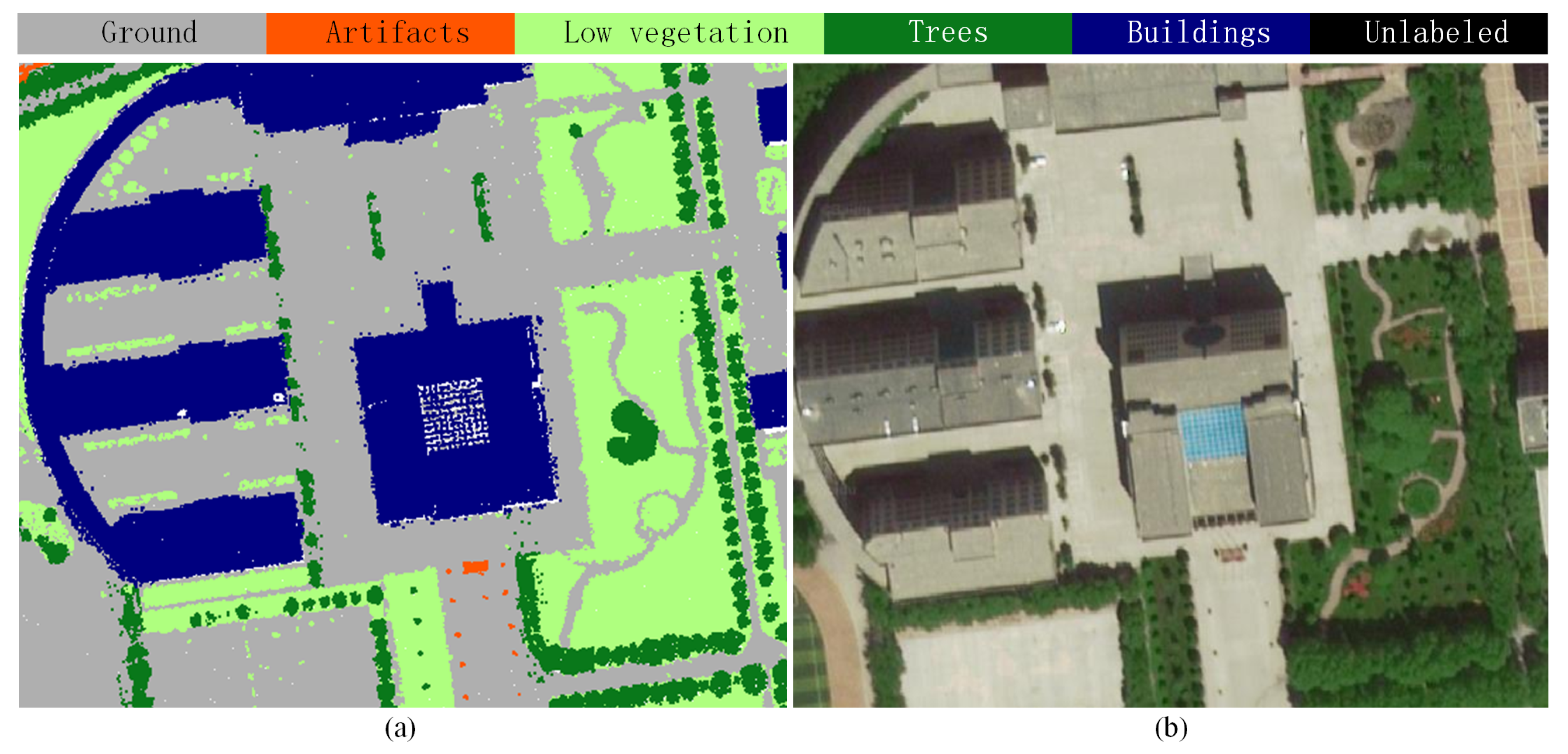
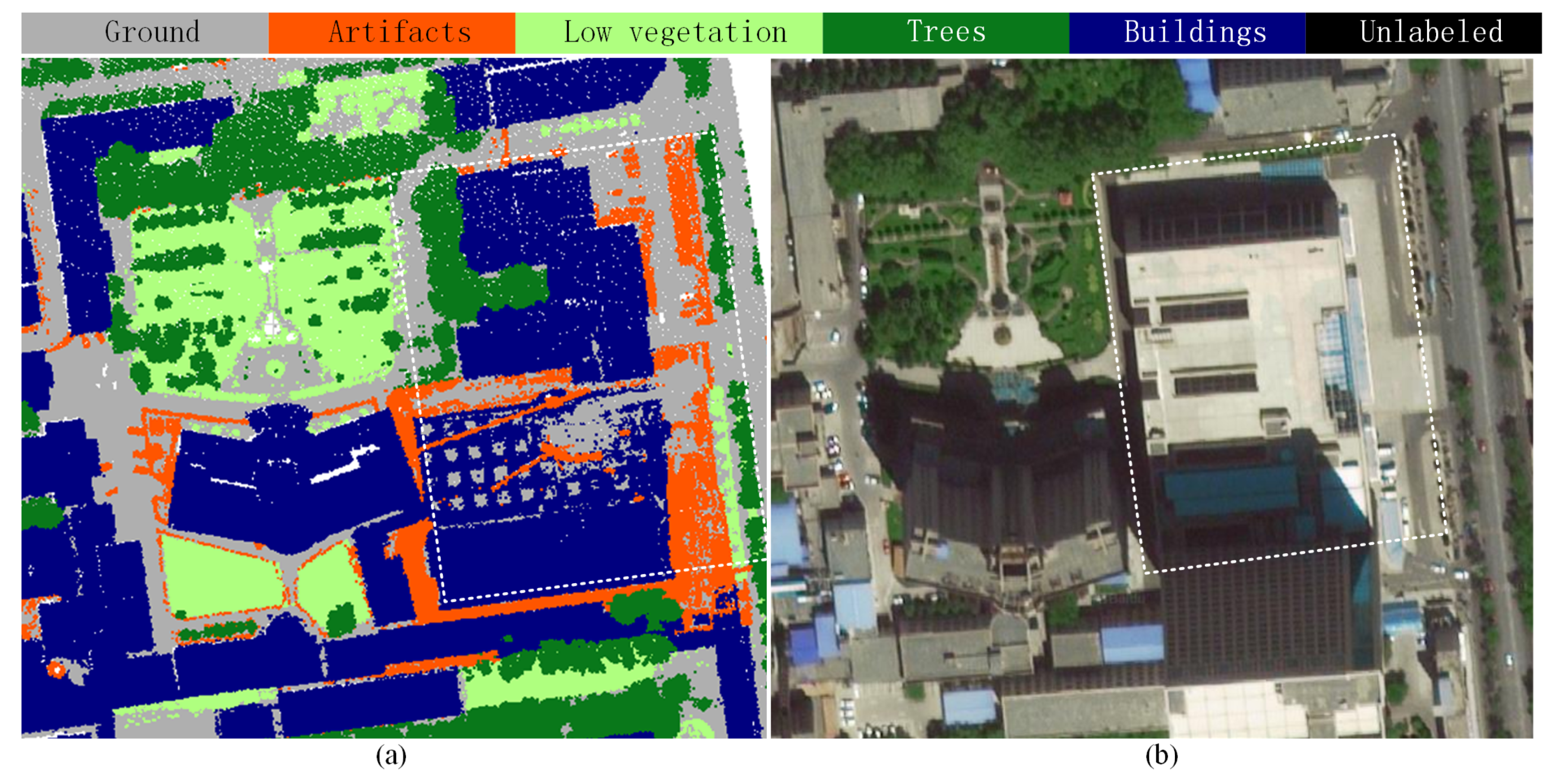
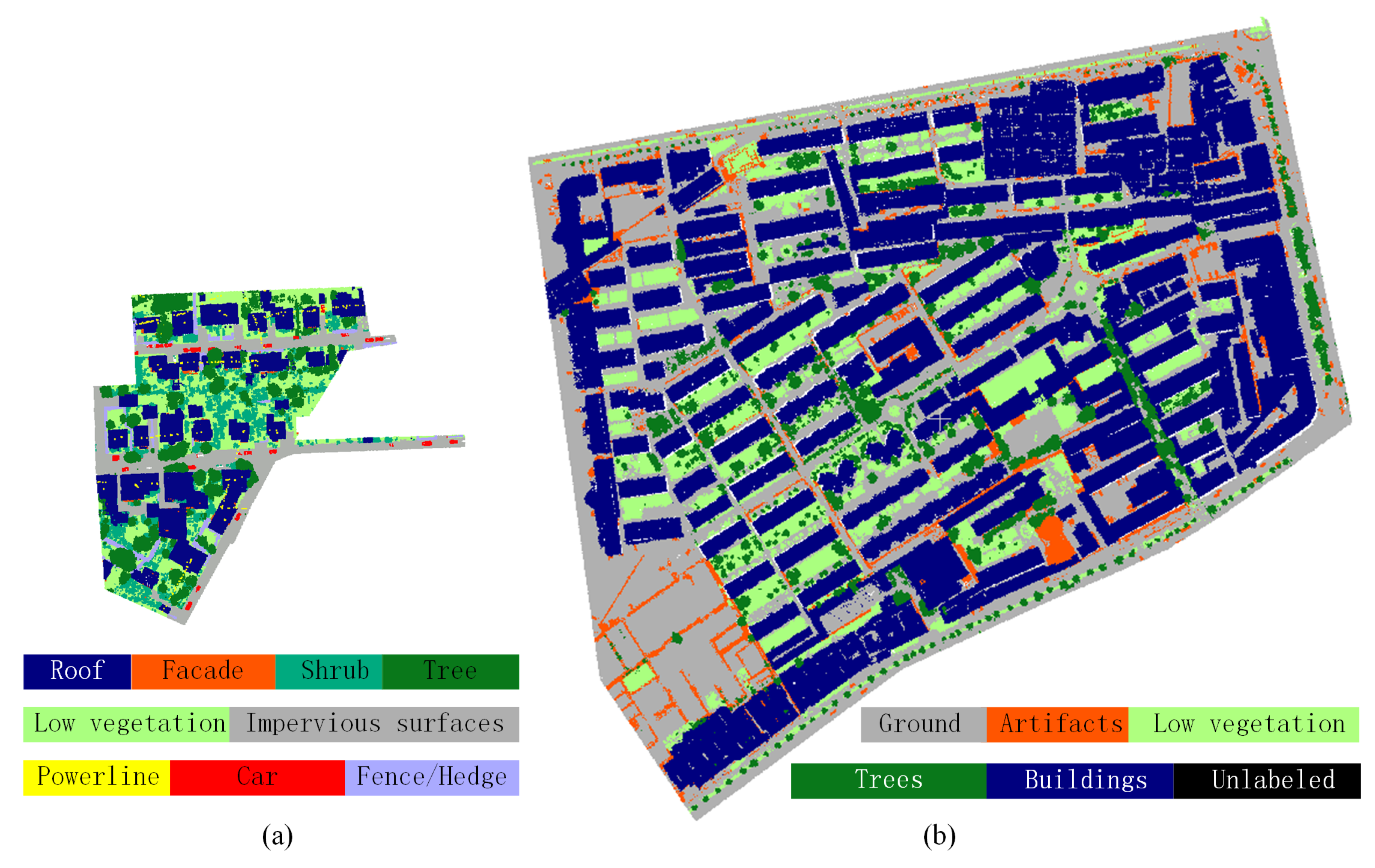
3. LASDU: Large-Scale Aerial LiDAR Point Clouds of Highly-Dense Urban Areas

Based on the analysis of the existing limitations and problems in the current benchmark datasets of ALS point clouds, we present a novel aerial LiDAR dataset, termed LASDU (Large-scale ALS data for Semantic labeling in Dense Urban areas), which is designed for the semantic labeling of ALS point clouds in highly-dense urban areas.

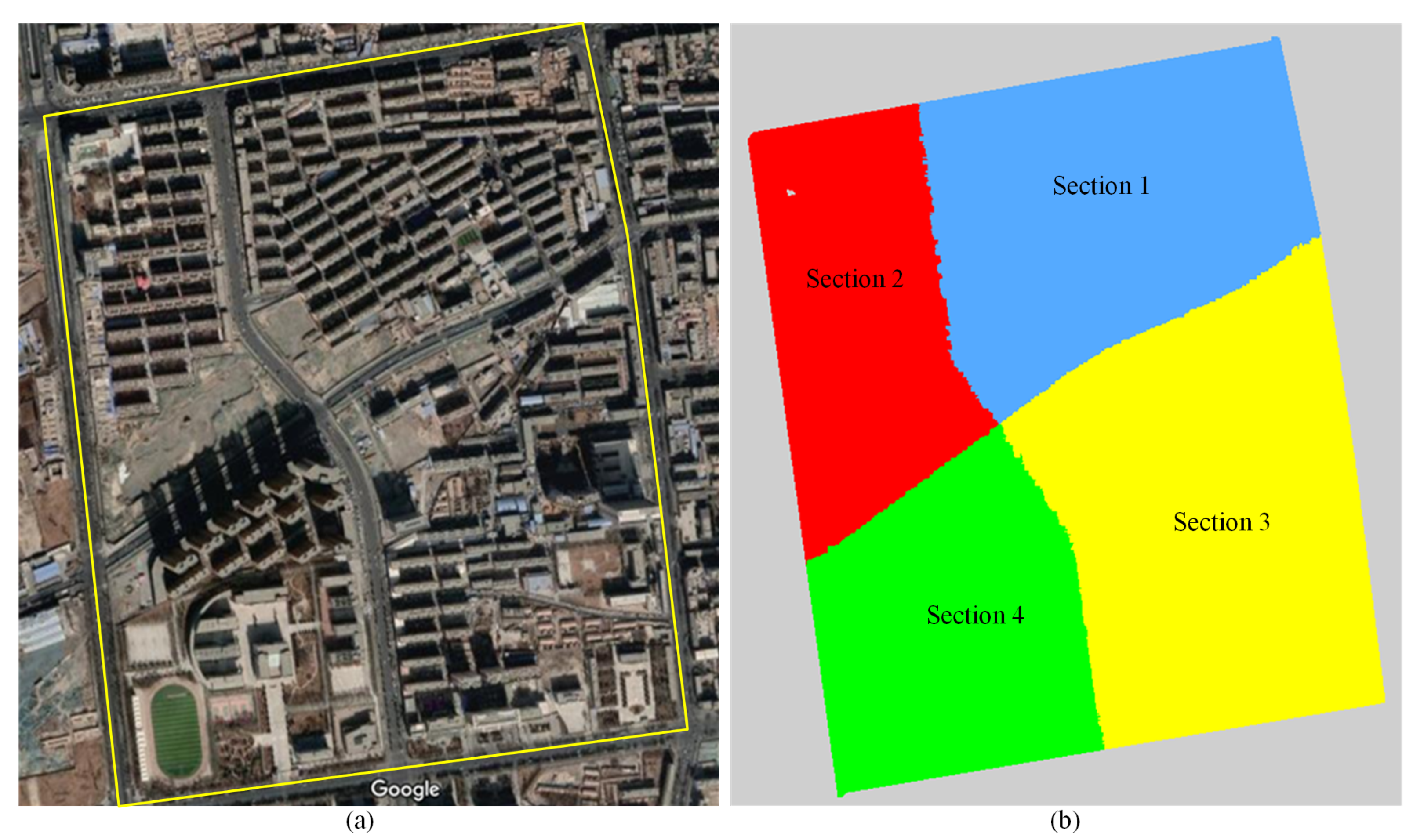
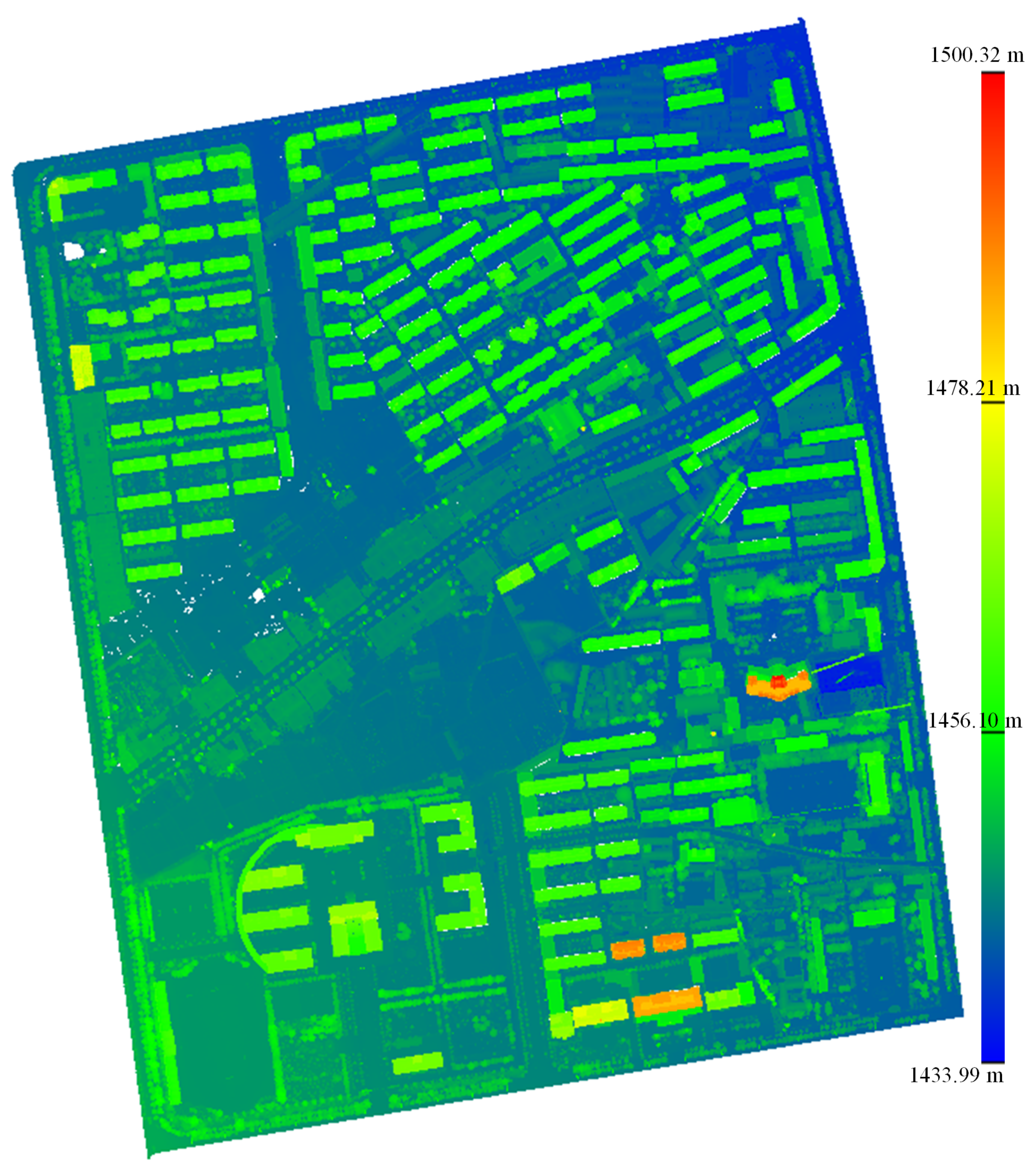
3.1. Data Acquisition

This dataset was a part of the data acquired in the campaigns from the HiWATER (Heihe Watershed Allied Telemetry Experimental Research) project [30]. The study area is in the valley along the Heihe River in the northwest of China. The topography in the study area is nearly flat, with an average elevation of 1550 m. The ALS point clouds were originally acquired in July 2012, by the use of a Leica ALS70 system onboard an aircraft with a flying height of about 1200 m. The geometric quality of this dataset has been given in the previous publication [31], which indicates that the average point density was approximately 3–4 pts/m² and the vertical accuracy ranged between 5–30 cm. The annotated dataset covers an urban area of around 1 km², with highly-dense residential and industrial buildings. In Figure 2, a height map of the dataset is shown, with the elevation of the study area given. From Figure 2, we can see that the annotated area is nearly flat and the maximum difference of elevation is only around 70 m, which is caused by the different heights of buildings.

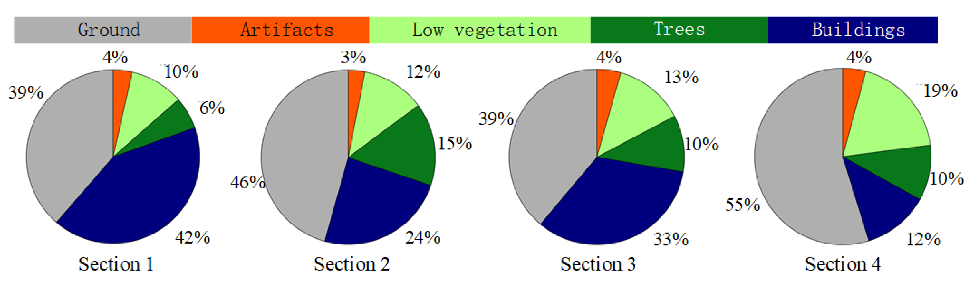
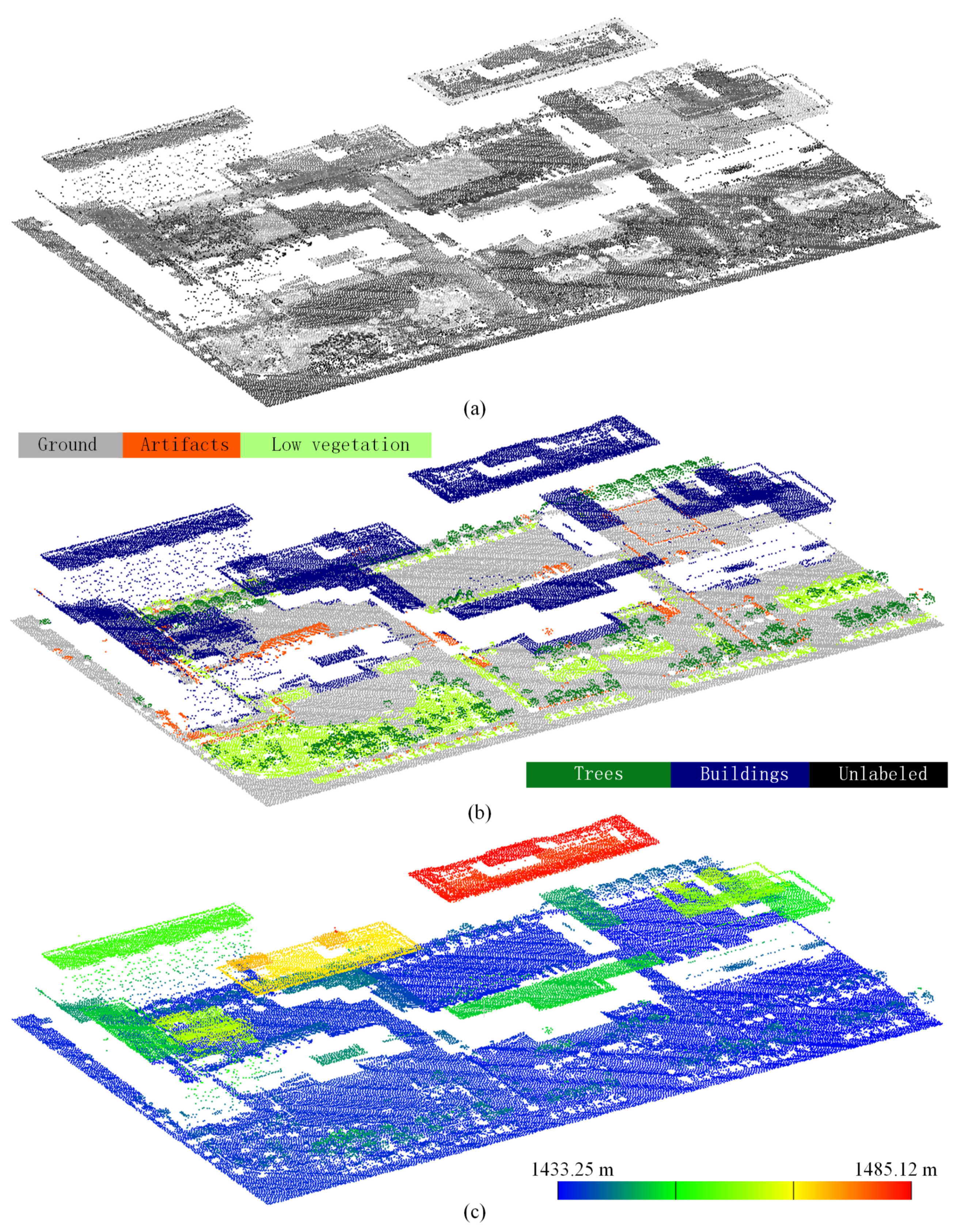
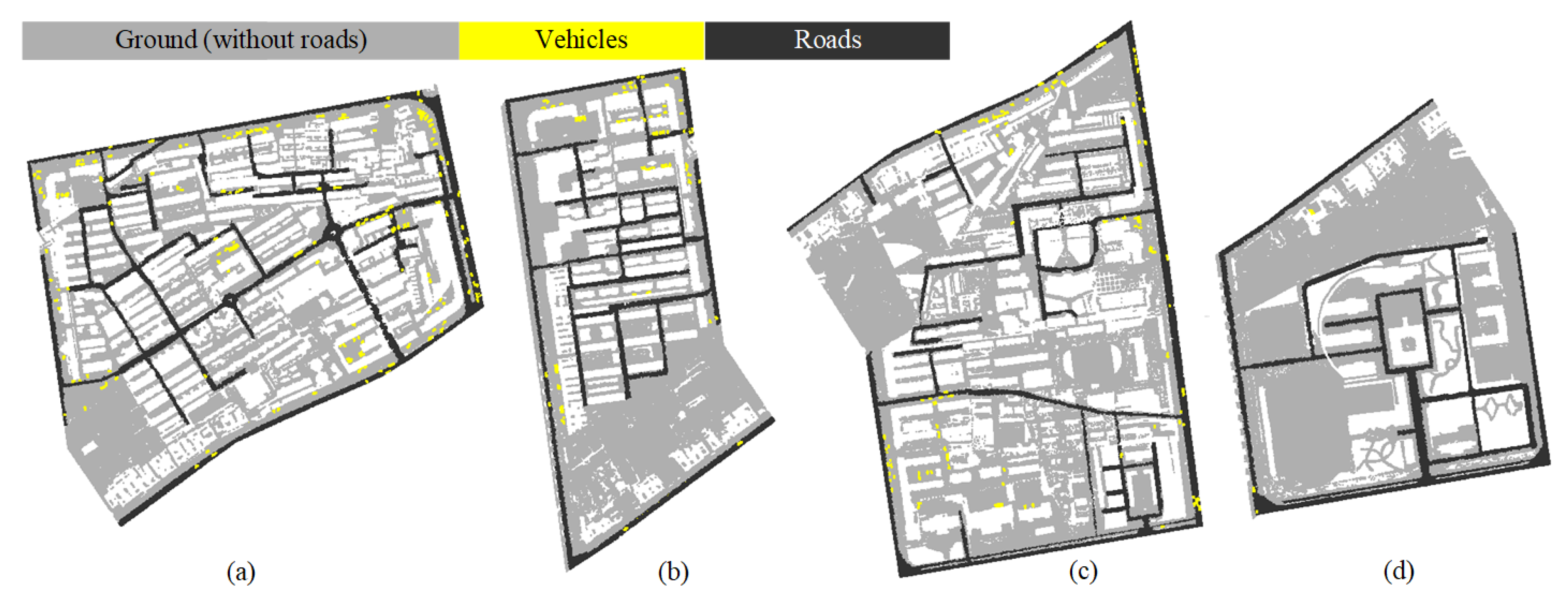
3.2. Data Description

The total number of annotated points is approximately 3.12 million. The entire labeled point cloud of the investigating area has been divided into four sections, and the numbers of points in these four sections total around 0.77 million, 0.59 million, 1.13 million, and 0.62 million, respectively. In Figure 3b, the separation of the study area is illustrated.

Points of the same section were saved separately in individual .las files. The separation and the annotation of points were manually carried out using CloudCompare 2.10 (https://www.danielgm.net/cc/) with point-wise accuracy. In the .las file, each point was assigned with the following seven attributes:

• Positions: Recording the 3D coordinates of each point, with the unit of meters in the UTM projection.
• Intensity: Recording the intensity of reflectance of each point, with a range between 0 and 255.
• Edge of flight line: Indicating a value of 1 only when the point is at the end of a scan.
• Scan direction: Denoting the direction of the scanner mirror when transmitting a pulse.
• Number of returns: Recording the number of multiple returns per transmitted pulses.
• Scan angle: Recording scan angle of each point in degree.
• Labels: Indexing object classes of each point, with an integer index from 0 to 5.

To gain a further impression of the data quality, the density of points and in different sections are analyzed in a statistical way. To compute the density of the points, the local point density (LPD) [32] of the point cloud is calculated:

$$\mathrm{LPD}=\frac{k}{\pi ·d_k^2}$$

(1)

where k is the number of involved neighbors and $d_k$ stands for the distance from the center point to its furthest neighbor, respectively.

In Figure 4, distributions of points densities indicated by LPD in different sections are given. In this figure, the horizontal axis denotes different LPDs of points, and the vertical axis stands for the number of points with a certain local point density. As seen from Figure 4, the point densities of these four sections generally concentrate at the LPD value of around 3 pts/m². The density of the point cloud of Section 3 is larger than those of Sections 1 and 2, reaching about 3.5 pts/m². This is mainly due to the high-rise buildings and trees, which provide a highly complicated object structure with more points scanned. In contrast, the point densities of Section 4 concentrate at the LPD value of only about 2.7 pts/m², which reveals a sparse point distribution caused by a simple scenario in this section. Generally speaking, we assume that the densities of points in this dataset are constant due to the fact that approximately fixed measuring distances of ALS will result in similar densities of points.

Regarding the annotation of points, we have manually labeled this area with five different classes of objects and one class of unclassified points, and points of different labels are rendered with different colors:

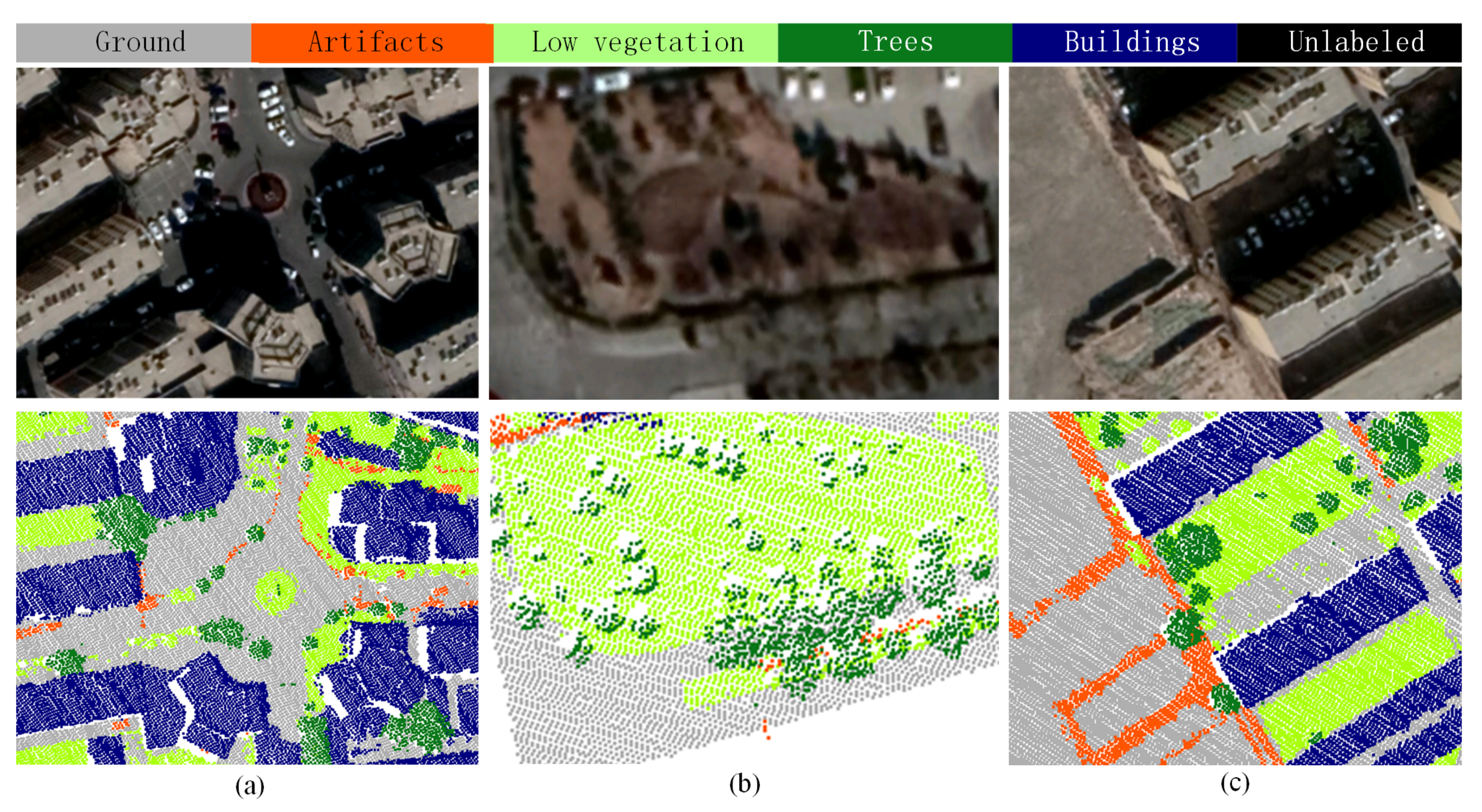
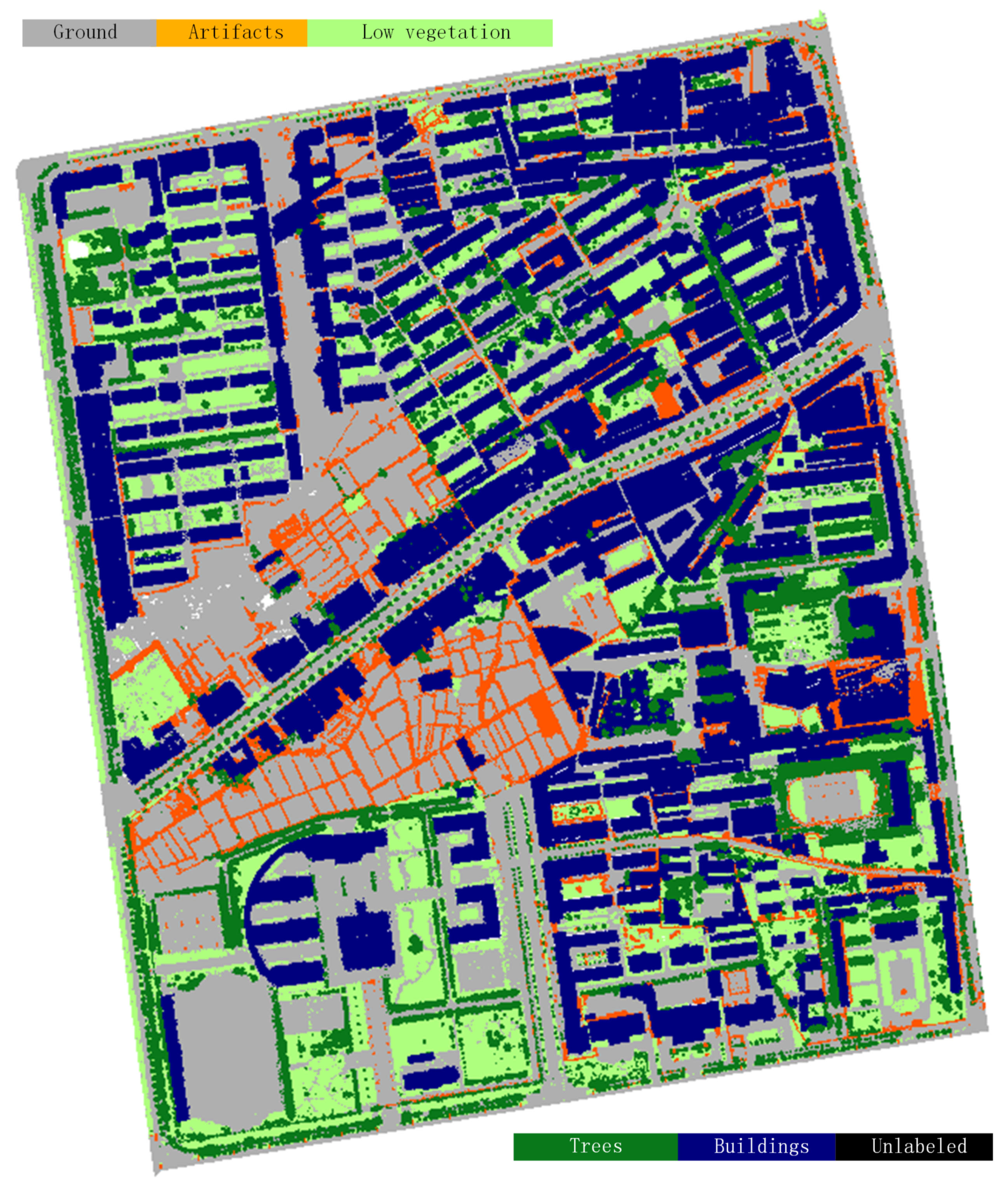
• Label 1: Ground (color codes: #AFAFAF): artificial ground, roads, bare land.
• Label 2: Buildings (color codes: #00007F): buildings.
• Label 3: Trees (color codes: #09781A): tall and low trees.
• Label 4: Low vegetation (color codes: #AAFF7F): bushes, grass, flower beds.
• Label 5: Artifacts (color codes: #FF5500): walls, fences, light poles, vehicles, other artificial objects.
• Label 0: Unclassified (color codes: #000000): noise, outliers, and unlabeled points.

In Figure 5, the statistics of the percentages of labeled points in different sections are given. From the statistics, we can find that for all four sections, the percentages of different objects show a similar tendency but in an unbalanced way. The ground points occupy the largest percentage at around 40% to 55%, while the percentage of building points ranks second with a value of around 30%, except for that of Section 4. The points of artifacts only reach about 4% among all the annotated points. The unbalanced distributions of percentages of labeled points in each section should be considered when trying to use them as training and testing datasets. It is recommended to use Sections 2 and 3 as the training data and to use Sections 1 and 4 as the testing data for the semantic labeling task.

In Figure 6, examples of annotated points of different objects compared with the objects in satellite images are given. As seen from Figure 6, we can clearly see that the highly-dense high-rise buildings directly neighbor each other, and they are always surrounded by low vegetation such as bushes and flower beds, which makes them difficult to separate. Moreover, trees are usually surrounded by bushes or are on grass. The most challenging part is the artifacts, which contain not only vehicles but also temporal short walls in the site of demolished buildings and hedges on bare land. These small objects have irregular shapes and have similar geometric features to bushes. In Figure 6c, we can even observe apparent differences between the measured point cloud and the satellite image due to the dynamic changes in this area.

In Figure 7, the labeled map of the ALS point cloud in the entire test area is given, with different objects rendered with various colors. All the highly-dense buildings, crowded trees, and irregular-shaped artifacts can be clearly observed, indicating the challenging task of semantically labeling all points in this scenario.

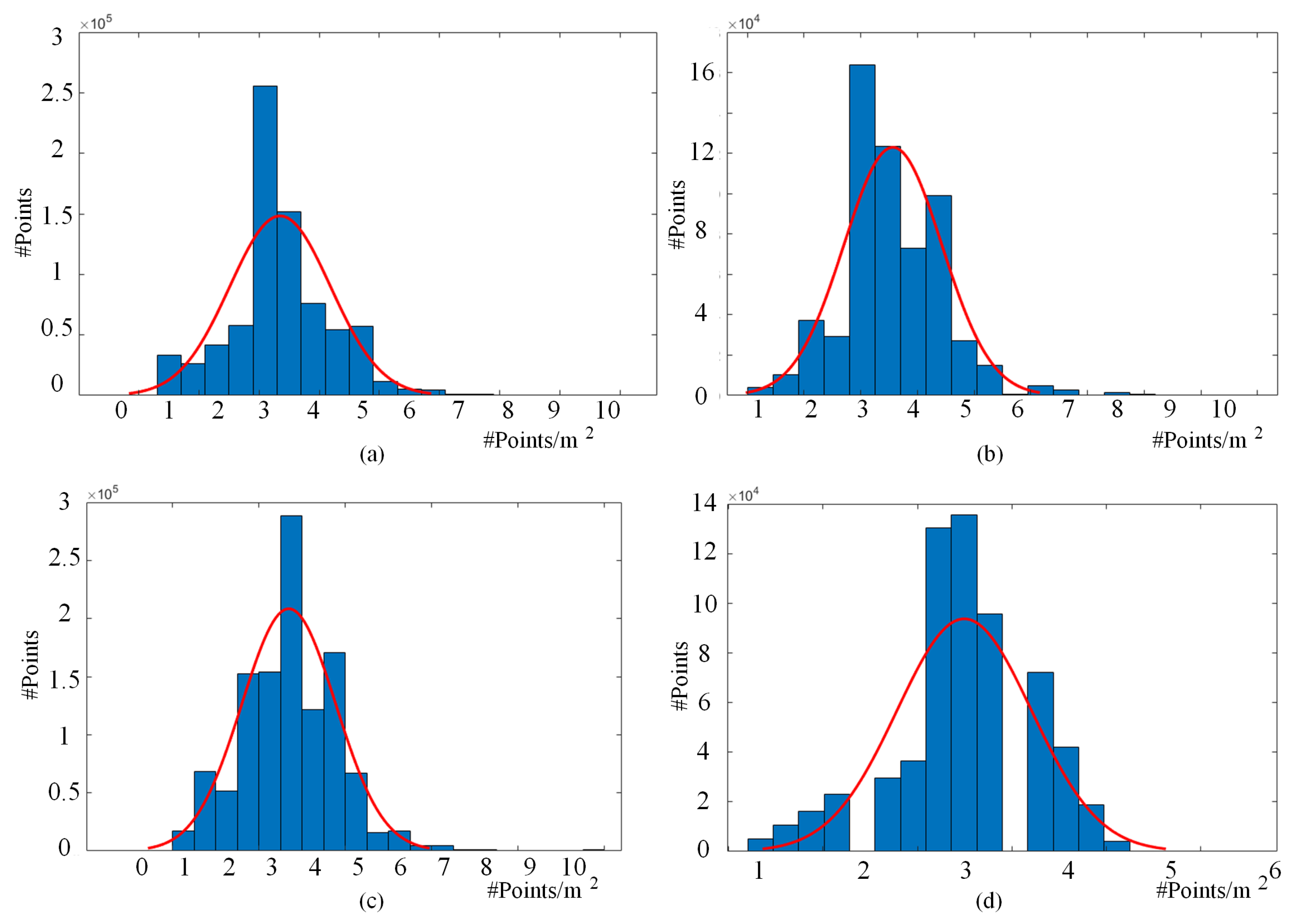
3.3. Features of the LASDU Dataset

For this dataset, the observed city blocks covered both the unchanged area and the changed area. The unchanged area is that in which the stable objects (e.g., road, buildings, tree) have not changed over the years when comparing the point cloud and the satellite image. Dynamic objects such as moving vehicles are not included. In Figure 8, we give an example of the unchanged area. Note that the point cloud was acquired in 2012, while the satellite image was taken in 2014. The changing area in this data mainly refers to construction sites. During the acquisition of the ALS point cloud, there were several on-going construction projects (for a single building or for an entire area). In Figure 9, we give an example of the changing area with a building finished during the time period between the acquisition of the point cloud and the satellite image. The position of this construction site is marked with a white dash box in the figure.

Moreover, in Figure 10, we provide a detailed view of the point cloud of the aforementioned construction site. The points are rendered with their intensity values. The status of this construction site was in the stage of building structures from the foundation pit. As seen from Figure 10, we can determine the points of cranes and an excavator. The formworks and steel-reinforced concrete structures in this foundation pit can also be observed. This would be of interest to the studies of object detection in the construction site from the ALS dataset.

Moreover, these construction sites also indicate that the investigated area has experienced a significant development with plenty of changes in both buildings and roads. A data set with changed buildings would be more interesting for change detection research. This is also a reason why we specially picked out and mentioned the area of construction sites in the dataset. Due to the situation that our presented dataset has no multi-temporal measurements, so it is impossible to conduct comparisons between point clouds for such change detection research. However, it would still be of value to conduct change detections between our presented ALS dataset and the newest satellite images from Google Maps, since the landscape has been drastically changed.

3.4. Significance of the LASDU Dataset

Compared with the existing ALS datasets, the major significance of the LASDU dataset is twofold: first, it provides a comparable large scale dataset in comparison with existing ones, especially for the most commonly used Vaihingen dataset; second, it covers a highly complex scenario which is challenging to label.

3.4.1. Comparable Large Scale Data Size

With regard to the size of the dataset, making a comparison to the renowned Vaihingen dataset, the LASDU dataset is from an urban outdoor scene collected by an aerial LiDAR system with an ALS sensor. However, LASDU. with a total area of approximately 1 km², is approximately four times as large as that of the Vaihingen dataset, covering around 0.4 km², and includes four times the number of points. Although the size of the coverage area in LASDU is smaller than DFC, DALES, and AHN3, it is still comparable to the size of DublinCity and better than our previous TUM-ALS dataset, which merely covered the region around the TUM city campus. On the one hand, a large dataset size meets the requirement of training deep-learning-based algorithms and methods; on the other hand, a large dataset will increase the challenge of efficiency, and this is more close to the real situation for large-scale urban mapping.

Regarding the number of labeled classes, the LASDU and Vaihingen datasets are both labeled with a similar number of classes for the purpose of semantic labeling, which is more detailed than TUM-ALS and AHN3 but inferior to the annotation of DublinCity and DFC. However, the core types of objects (i.e., buildings and vegetation) considered in urban mapping tasks have been included in LASDU. A detailed annotation will facilitate the semantic interpretation of the urban scene, but the increasing cost will be unacceptable and the implementation of manual labeling will be infeasible [11]. Regarding the density of points, the DublinCity dataset has a much higher point density than ours, and a higher point density will improve tasks such as 3D reconstruction in urban scenarios. However, measured point clouds with such a high density are not commonly available data sources for practical large-scale city mapping, especially for applications in developing countries. Moreover, the high density of measured points will increase the cost of mapping and the difficulties of annotation; thus, the presented LASDU dataset features a large-scale data size while having a reasonable number of labeled classes and point density.

3.4.2. Challenging and Complex Scenarios

In contrast to other datasets, the LASDU dataset is characterized by its challenging and complicated scenario, bringing more challenges to conducting the adequate semantic labeling of points. This also provides a more critical evaluation of the developed methods and algorithms. The LASDU dataset covers an area full of highly-dense buildings. Unlike the even distribution of buildings in the Vaihingen dataset, the LASDU dataset has more substantial variations of building densities; namely, in some areas, there is a very high density of buildings, while other places only have sparse infrastructure but dense trees and bushes. Moreover, compared with the residential areas recorded in TUM-ALS, DublinCity, and DFC datasets, the LASDU dataset scanned a hybrid area. The types of buildings included by the LASDU dataset vary from residential buildings to industrial ones, and the dataset even records the construction sites with dynamic changes. All these increase the challenges of developing robust and effective semantic labeling methods. More importantly, all the buildings are located in a closely-packed way, and the average distance between nearby buildings is only around 5 m, which is much smaller than the situation in TUM-ALS and AHN3. Even comparing the newest DALES dataset, the density of hi-rise buildings in our LASDU dataset is still much higher. The buildings in LASDU are located side by side. The short distance between buildings directly increases the difficulty of labeling and separation. In Figure 11, we give a comparison of the building distributions of two sections from the Vaihingen and LASDU datasets, and from the comparison, we can clearly observe the highly-dense buildings in the LASDU dataset. These dense buildings with small and narrow rectangular shapes will greatly increase the difficulty of labeling. Furthermore, in the recorded scenario, not only do the adjacent buildings arouse challenges but so do the low vegetation and vehicles, especially in areas where they overlap with poles and trees and are close to buildings. Besides, the short ridges on the bare land and walls hidden in various wall-like vertical structures are also challenging to identify. Actually, the LASDU dataset has also marked parking vehicles in the class of artifacts, which could further be utilized in tasks such as vehicle detection. However, limited by the point density, a scanned vehicle merely consists of 8–10 points, which increases the difficulty of detection and extraction.

3.4.3. Potential Use for Traffic-Related Applications

Since the LASDU dataset is originally designed for applications such as urban mapping and 3D reconstruction of buildings, so we focused more on the vegetations and buildings that are scanned in the point clouds, when we design the categories of objects that are needed to be annotated. However, traffic-related applications have attracted increasing attention when applying point clouds in an urban scenario. It means that roads and vehicles are also interesting categories of objects which may give their importance in related applications.

To this end, to further explore the potential of being used in traffic-related applications, we also provide a refined categorization of point cloud annotation based on the five existing categories, although the ALS dataset is not an adequate data source for traffic-related applications due to the sparse point density and occlusions caused by high-rise buildings and trees in a nadir view observation. Specifically, we separated points of “roads” from points of ground, and we extract points of vehicles from points of artifacts. These points are annotated with unique labels, and it is an option to use these labels in tasks such as road detection or vehicle extraction. In the semantic labeling task, they are still regarded as parts of ground or artifacts, respectively. In Figure 12, we illustrate the annotated points of these two new categories of objects. The annotation of roads is guided by Google Maps and visual inspections manually.

4. Experimental Evaluation

To give a brief evaluation of the proposed dataset, we applied this dataset in supervised classification to label the points with the five aforementioned classes of objects in the scene.

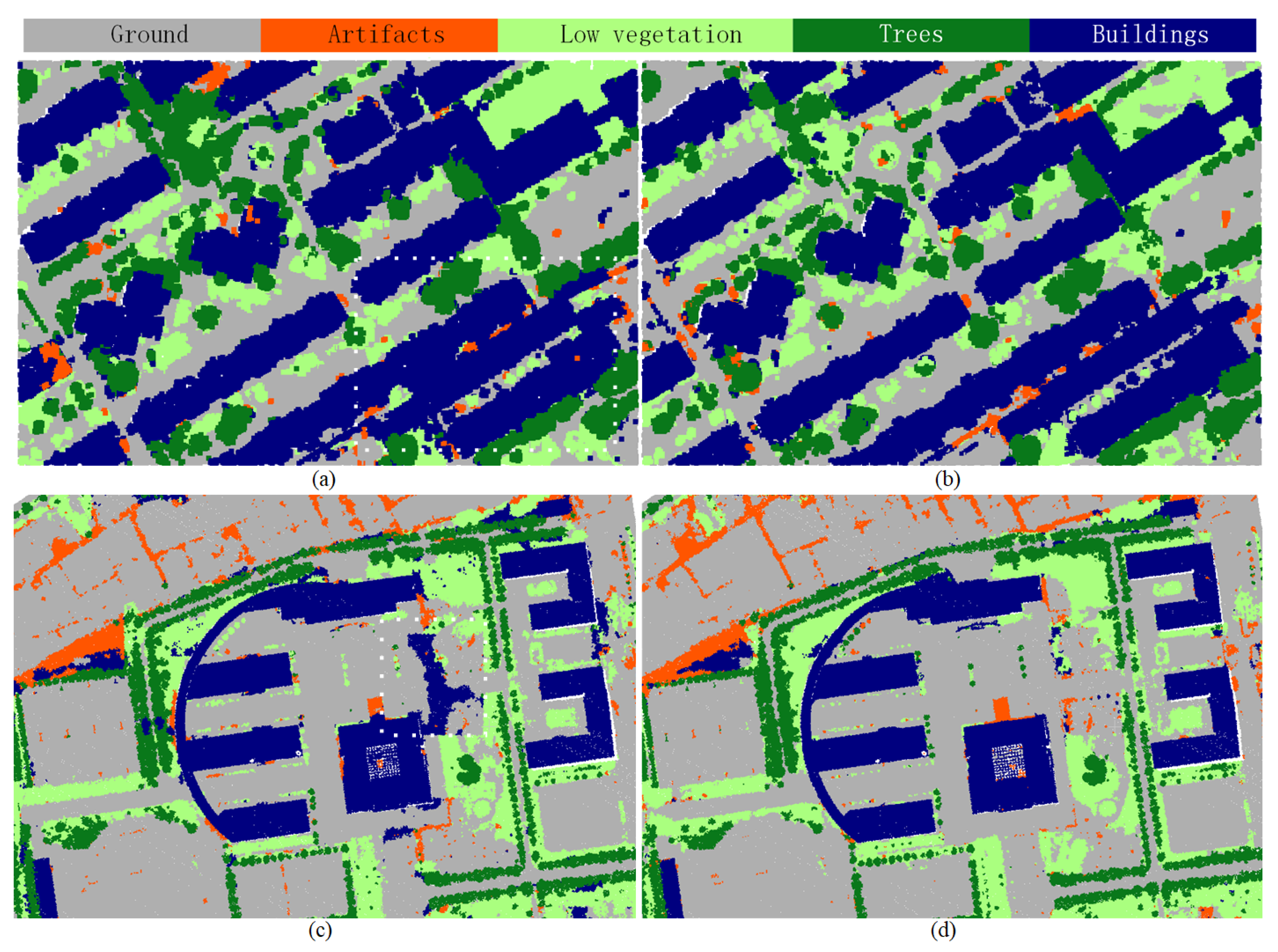
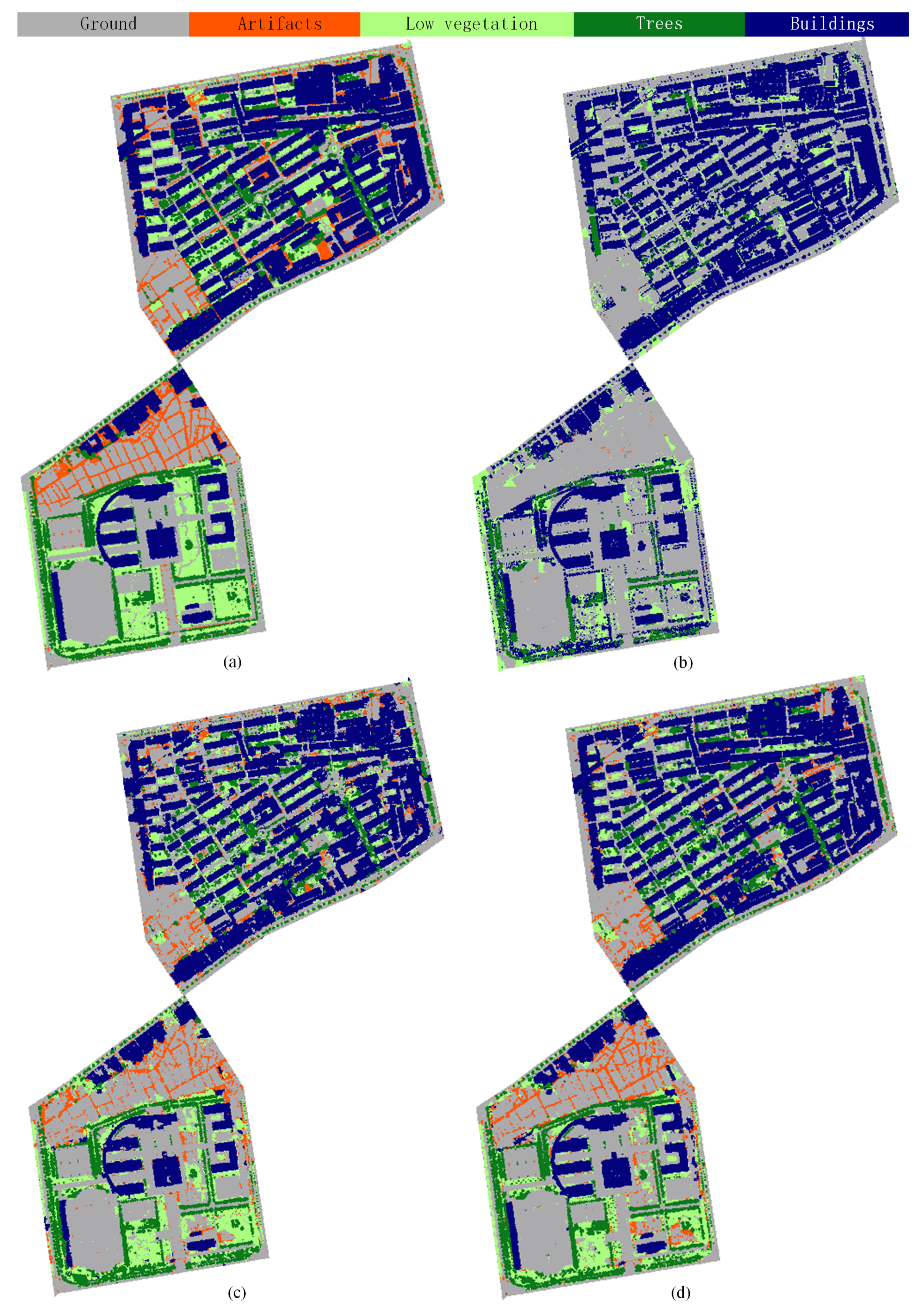
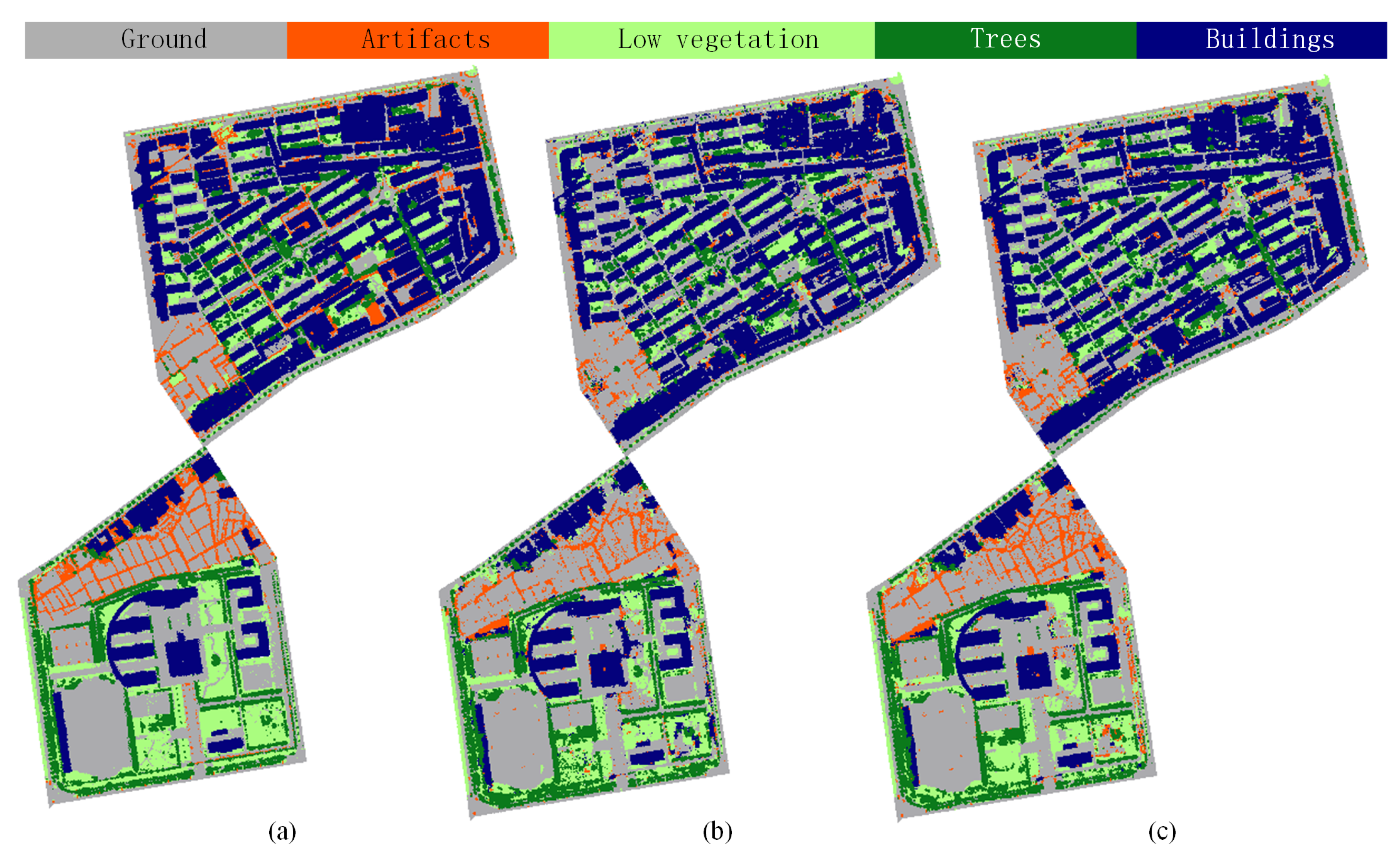
4.1. Semantic Labeling Experiments

In contrast to common indoor applications in the computer vision field, semantic labeling in large-scale urban areas should consider the changes of object scales. In the outdoor scenario, for objects of different dimensions, the encoded features will vary greatly along with the size of local neighborhoods [18] or the sampling scale [13]. Especially for the dense urban area, closely-packed buildings will arouse an incorrect determination of the scales in some adaptive methods. Our proposed dataset is a case with both a large scale and highly-dense areas with closely-packed buildings. Thus, in the evaluation experiments, three point-based semantic labeling methods are selected and tested on the proposed dataset as baselines. All these three methods are deep learning-based, but they use different strategies to cope with the scale problems, which directly links to the highly-dense urban scenarios.

• PointNet [33]: PointNet is a neural network that directly works with point clouds and respects the permutation invariance of points in the input well. It provides a unified architecture for applications ranging from object classification to semantic segmentation.
• PointNet++ [34]: PointNet firstly learns global features with MLPs with raw point clouds. PointNet++ applies PointNet to local neighborhoods of each point to capture local features, and a hierarchical approach is taken to capture features with multi-scale local context.
• Hierarchical Data Augmented PointNet++ (HDA-PointNet++): This is an improved method based on the original PointNet++, which was proposed in the previous work [13] as the multi-scale deep features (MDF) in the context of hierarchical deep feature learning (HDL) method. It was developed based on a hierarchical data augmentation strategy, in which sizable urban point cloud datasets are divided into multi-scale point sets, enhancing the capability of dealing with scale variations. This hierarchical sampling strategy is a trade-off solution for object integrity and fine-grained details.

For the HDA-PointNet++ method, in Figure 13, we give an illustration for the workflow of HDA-PointNet++. In the previous work [13], it is also termed as MDF in the HDL method, in the training stage of which the input point cloud will experience three-fold subdivisions with various scales repetitively. All the subsets of points will be then downsampled and fed into the PointNet++ network for training, ensuring a stronger generalization ability when dealing with widely varied-scales of different objects. However, it is noted that the point clouds for testing are directly fed to the network without subdivision and downsampling, which is different from the HDL step in [13].

In the experiments, we use Sections 2 and 3 as the training data, and use Sections 1 and 4 as the testing data. As points in our dataset are equipped with not only 3D coordinates but also other attributes such as intensities, we conducted two groups of experiments. The first group uses only the 3D coordinates of points with all the three methods, which is designed to assess the 3D geometric performance of points in the dataset; in the second group, the intensity values of points in the dataset are involved in the experiments using two methods (i.e., PointNet++ and HDA-PointNet++), with the aim of checking the influence of radiometric information in the semantic labeling. Moreover, the influence of the aforementioned scale problems for all three methods will be analyzed and discussed.

4.2. Evaluation Metrics

The evaluation metrics include the precision ($Pre$), the recall ($Rec$), the F1 measure ($F1$), the overall accuracy ($OA$) and averaged $F1$ measures ($\mathrm{Avg}F1$), which follow the ISPRS benchmark dataset of 3D semantic labeling [7]. The precision ($Pre.$) and recall ($Rec.$) values are also given to assess the performance, based on the calculated $TP$, $FP$, and $FN$. $TP$ refers to the true positive for the labeled outcome of a class, which is the number of points properly labeled as that class, namely those with the appropriate mark. $FP$ represents the false positive, indicating the number of points with the wrong mark. $FN$ is the false negative, which is the number of points that should be marked as other classes but are incorrectly marked. The evaluation measure for class i is defined as

$${F1}_i=\frac{2T{P}_i}{2T{P}_i+F{P}_i+F{N}_i}.$$

(2)

The evaluation measurement for the entire classification result is $\mathrm{Avg}F1$, which is the average summation of ${F1}_i$ for each class i.

$$\mathrm{Avg}F1=\frac{1}{N}\sum _{i=1}^N{F1}_i.$$

(3)

Finally, the overall accuracy ($OA$) is calculated as well.

$$OA=\sum _{i=1}^N\left(\frac{T{P}_i}{T{P}_i+T{N}_i+F{P}_i+F{N}_i}\right).$$

(4)

5. Results and Discussions

5.1. Preprocessing and Training

As the preparation for training deep neural networks for all the methods, a fixed number of points were sampled as formatted subsets as inputs. As a consequence, point clouds of training and test datasets were subdivided into subsets with no overlaps.

For the experiment using only 3D coordinates, each point in a subset was represented by a 3D vector with x-, y-, z-coordinates, whereas for the experiment using additional intensities, each point in the subset was structured as a 4D vector with x-, y-, z-coordinates and intensity. The number of sampled points in each subset was set to the same as that in [13]. Namely, 8192 points were chosen without replacements from each subset of points in PointNet and PointNet++ methods, while when implementing the multi-scale strategy in the HDA-PointNet++ method, we generated subsets of points with different scales. The training of networks with these subsets of points with different scales was carried out individually as well. Thus, we were able to acquire encoded features encapsulating different levels of contextual information from points. Considering the real scale of objects (e.g., buildings, trees, low vegetation), the sizes of the subset of points were empirically set to 10,000, 20,000, and 30,000 for different scales, respectively, since they showed satisfying performance in the experiments.

To validate and supervise the training process, 10% of the training samples from the training datasets were selected directly for validation. In the training process, an Adam optimizer with an initial learning rate of 0.001, a momentum value of 0.9, and a batch size of 16 were used. The learning rate was iteratively reduced on the basis of the current epoch by a factor of 0.7. The training process lasted for 500 epochs in total, meaning the termination condition of the training process was determined by 500 epochs. The weights were saved if the training loss apparently decreased. Furthermore, the models were selected according to the highest OA on the validation set. Regarding the hardware used in the experiments, the training and testing of the deep neural networks were implemented via TensorFlow and ran on an NVIDIA TITAN X (Pascal) 12 GB GPU.

5.2. Classification Results of LASDU Dataset Using Only Point Positions

The first group of experiments was conducted with 3D coordinates of points without using other attributes, which was purely based on the geometric features of points. We finally achieved an OA of 83.11% for labeling the five classes with the HDA-PointNet++ method in our LASDU dataset. Additionally, we provided a comparison with the other two methods, which revealed that, considering the multiscale strategy, the HDA-PointNet++ method was able to outperform the other two baselines.

Table 2. Comparison of classification results using the LASDU dataset (no intensities) with different semantic labeling methods (all values are in %).

Methods	Metrics	Artifacts	Buildings	Ground	Low_veg	Trees	$\mathit{OA}$	$\mathbf{Avg}{\mathit{F}}_1$
PointNet [33]	$Pre$	63.64	85.34	57.52	20.96	42.43	63.02	44.04
	$Rec$	00.02	62.34	97.46	06.89	03.79
	$F1$	31.83	73.84	77.49	13.92	23.11
	$Pre$	28.65	90.09	58.44	38.18	78.53	65.19	51.09
PointNet++ [34]	$Rec$	14.26	63.55	91.32	19.34	28.53
	$F1$	21.45	76.82	74.88	28.76	53.53
	$Pre$	41.46	93.55	83.17	63.92	84.56	83.11	71.70
HDA-PointNet++ [13]	$Rec$	34.58	94.86	91.24	43.50	86.41
	$F1$	37.87	94.20	87.20	53.71	85.49

lists the classification results of all these three methods. Concerning the overall accuracy, we could observe that the HDA-PointNet++ using multiscale deep features could primarily improve the performance of classification with an increment of OA by around 17%, compared with PointNet++. This is because, for the point-based deep neural network, the subdivision and sampling of point clouds in large urban scenes is an important issue that directly affects the classification results. PointNet, which uses single-scale deep features, has difficulty handling urban objects with various scales. As an improvement, PointNet++ introduced sampling and grouping with different scales, which could improve the classification results. Since the subdivided point sets were the basis for providing the contextual information from the clustering of points, the scales of each point set needed to be tested and investigated. Instead of searching for the optimal scale size for the subdivided point sets, we used a compromise strategy. Here, the HDA-PointNet++ method compared the extracted deep features using a hierarchical subdivision strategy with the features extracted directly from the network. With the application of the hierarchical subdivision strategy, some wrongly classified areas could be corrected. Compared with the single-scale methods, the multiscale features performed better in the classification results, both in terms of the statistics of accuracy and the visualization in the classification map.

The visualized classification results are shown in Figure 14. It can be seen that the result of PointNet++ showed good performance, which indicates the efficacy of the deep neural network in providing productive features. It can also be observed that the different methods show completely varied outputs. In particular, for the category of artifacts with highly complicated objects, PointNet hardly obtains any correct result for the ridges on the bare land; in contrast, PointNet++, by introducing the sampling and grouping strategy, becomes sensitive to objects at both the small and large scale, and so such small and complex artifacts can be correctly labeled. However, for the low vegetation and trees among the highly-dense buildings, PointNet++ failed to deal with these cases. In contrast, the HDA-PointNet++ method with a hierarchical structure can handle this issue in a more robust and adaptive way. Therefore, it can be concluded that the multiscale deep features provide higher descriptiveness. On the other hand, from the aspect of the dataset, we can also comment that our LASDU dataset is more challenging than the classic ISPRS benchmark dataset, although it has more categories of objects. However, such complex urban scenarios are more frequent cases when we conduct large-scale 3D mapping in residential areas.

5.3. Classification Results of LASDU Dataset Using Additional Point Intensities

As the intensity of the point is reliable information and frequently used in many LiDAR data applications, the second group of experiments was conducted with 3D coordinates of points with intensities, the results of which were based on both the geometric features and radiometric attributes of points. In this experiment, we compared the results of PointNet++ and HDA-PointNet++ methods. Finally, to label the five classes of objects in our LASDU dataset, we achieved OA values of 82.84% and 84.37%, respectively.

Table 3. Comparison of classification results using the LASDU dataset (with intensities) with different semantic labeling methods (all values are in %).

Methods	Metrics	Artifacts	Buildings	Ground	Low_veg	Trees	$\mathit{OA}$	$\mathbf{Avg}{\mathit{F}}_1$
PointNet++ [34]	$Pre$	34.74	91.44	85.83	66.77	78.38	82.84	70.96
	$Rec$	27.78	89.82	89.65	59.58	85.59
	$F1$	31.26	90.63	87.74	63.17	81.98
HDA-PointNet++ [13]	$Pre$	38.66	95.91	85.73	69.47	79.98	84.37	73.25
	$Rec$	35.11	90.40	91.75	61.01	84.51
	$F1$	36.89	93.16	88.74	65.24	82.24

lists the detailed classification results of these two methods. As seen from the table, we can see a considerable increase in the classification accuracy of PointNet++, with an increase of OA of more than 15%. This is mainly due to the increased accuracy regarding low vegetation. By introducing intensity, as objects of low vegetation always have different intensities compared with those of man-made artifacts, the points of these two classes are easier to separate. The results of HDA-PointNet++ show that it experienced a slight increase of OA by around 1%, which is not particularly significant. This is due to the fact that the hierarchical data sampling and augmentation in HDA-PointNet++ have fully explored the potential of this method, meaning that the intensities barely make further contributions to the improvement of accuracy.

Additionally, the visualized classification results are given in Figure 15. As can be seen, the performance of PointNet++ significantly improved, which indicates the contribution of using intensities. The correctly labeled points of grass and ridges on the bare land can be clearly observed. Moreover, trees and bushes crowded by the closed compacted buildings can be separated and labeled as well. Similarly, the HDA-PointNet++ method with a hierarchical structure reveals a similar quality of results. Therefore, as a conclusion, we can comment that for semantic labeling on our LASDU dataset acquired in a highly complicated building area, not only do the geometric features play a vital role but also attributes such as intensities can contribute to distinguishing points of various objects. This also provides an indicator of using our dataset in the evaluation of a newly proposed method. In Figure 16, we also selected two example areas from Sections 1 and 3 (i.e., testing data) to illustrate the details in the dense building areas crowded with trees and low vegetation. It is apparent that when the intensity values added to the input data, both two methods can achieve satisfying classification results for buildings, grounds, and trees. However, for the results obtained from original PointNet++, there are more insulated incorrectly labeled points for low vegetation and artifacts, while for the independent buildings, they are wrongly recognized as connected ones (see adjacent buildings in the white dash box of Figure 16a). For the HDA-PointNet++ method considering the scale factor, labeled points can likely keep a clear and smooth border for individual objects, e.g., the border between buildings and trees and the boundaries between the trees and low vegetation. Moreover, since the scales of the trees and buildings vary significantly, the result of HDA-PointNet++ can avoid the large and continue errors when labeling points of buildings (see the area in the white dash box of Figure 16c). This is particularly of value when mapping the urban scenario from ALS data.

5.4. Discussion on Hierarchical/Multi-Scale Strategy for Large-Scale Urban Semantic Labeling

According to the above two groups of experiments, we can see that the HDA-PointNet++ method with a hierarchical data augmentation strategy represents a significant improvement over the original PointNet++ method, although they have the same core network structure. As we have mentioned before, the scale plays a role in both the geometric and radiometric description of the object. An inappropriate scale of sampling can only partially represent the object, resulting in an incomplete or over-covered feature description, the multi-scale augmentation of input data has increased the generality of the trained neural network, which makes the encoded features adaptive to the scale of the object. The complex scenario with dense and crowded buildings in our dataset increases the difficulty and highlights the contribution of the multiscale strategy. However, on other classic benchmark datasets—for example, the Vaihingen dataset—the methods utilizing a hierarchical or multi-scale strategy also show promising performance. We have collected and compared the results of classification methods including LUH [35], PointNet++ [34], multi-scale convolutional neural network (MCNN) [36], rectified linear units neural network (ReLu-NN) [37], PointNet on multiple scales (PointNet-MS) [38] deep point embedding (DPE) [13], geometry-attentional network (GA-Conv) [39], and voxel and pixel representation-based networks (VPNet) [40], and we can see that for methods that work directly on 3D points, those (e.g., LUH, DPE, and GA-Conv) utilizing a hierarchical or multi-scale strategy show noteworthy performance. For example, the GA-Conv method proposed a dense hierarchical architecture and elevation-attention module and achieves a promising result. Moreover, the VPNet method, assembling both pixels and voxels, also considers the representations of different scales and connects isolated individual points and obtained excellent performance with an average F1 score of 73.9%. All these results indicate that the scale factor considered via a multi-scale or hierarchical strategy contributes to outdoor semantic labeling, especially for dense and complex urban scenes, which is slightly different from the indoor cases. Thus, we can comment that not only should the classic methods using handcrafted features consider the multi-scale strategy when identifying the local neighborhood estimating features [18], but also the deep learning-based methods should consider the scales in the data input or directly in the neural network design.

6. Conclusions

In this paper, we present a large-scale aerial LiDAR point cloud dataset acquired in a highly-dense urban area for the evaluation of semantic labeling methods. This dataset covers a metropolitan area with highly-dense buildings of approximately 1 km² and includes more than 3 million points. This dataset was manually annotated into five categories of objects: ground, buildings, trees, low vegetation, and artifacts. With similar features and categorization of annotated points but more challenging scenarios and a larger size, this dataset is significant complementary for the commonly used ISPRS 3D semantic labeling dataset. Experiments were carried out with results from several baseline methods. As a conclusion, we can remark that the proposed LASDU dataset reveals the feasibility and capability of it serving as a benchmark for assessing semantic labeling methods. Moreover, the conducted experiments provide an evaluation of deep learning-based methods considering various scale strategies, meaning that the influence of scale factors in the deep neural network for point cloud semantic labeling in a scenario in which objects have different geometric sizes is analyzed. The LASDU dataset provides a new ALS benchmark dataset in a highly complicated urban scene with highly-dense buildings. The intention of presenting this new point cloud dataset is to encourage the development of practical and innovative semantic labeling methods for municipal applications. In the future, the dataset will be released for community access, and the categories and labels of this new dataset could be improved and updated with feedback from further experiments and evaluations.

References

1. Vosselman, G.; Maas, H.G. Airborne and Terrestrial Laser Scanning; CRC Press: Boca Raton, FL, USA, 2010. [Google Scholar]
2. Xie, Y.; Tian, J.; Zhu, X. Linking Points With Labels in 3D: A Review of Point Cloud Semantic Segmentation. IEEE Geosci. Remote Sens. Mag. 2020. [Google Scholar] [CrossRef] [Green Version]
3. Chen, S.; Nan, L.; Xia, R.; Zhao, J.; Wonka, P. PLADE: A Plane-Based Descriptor for Point Cloud Registration with Small Overlap. IEEE Trans. Geosci. Remote Sens. 2019, 58, 2530–2540. [Google Scholar] [CrossRef]
4. Dong, Z.; Yang, B.; Liang, F.; Huang, R.; Scherer, S. Hierarchical registration of unordered TLS point clouds based on binary shape context descriptor. ISPRS J. Photogramm. Remote Sens. 2018, 144, 61–79. [Google Scholar] [CrossRef]
5. Dong, Z.; Liang, F.; Yang, B.; Xu, Y.; Zang, Y.; Li, J.; Wang, Y.; Dai, W.; Fan, H.; Hyyppä, J.; et al. Registration of large-scale terrestrial laser scanner point clouds: A review and benchmark. ISPRS J. Photogramm. Remote Sens. 2020, 163, 327–342. [Google Scholar] [CrossRef]
6. Munoz, D.; Bagnell, J.A.; Vandapel, N.; Hebert, M. Contextual classification with functional max-margin markov networks. In Proceedings of the 2009 IEEE Conference on Computer Vision and Pattern Recognition, Miami Beach, FL, USA, 20–26 June 2009; pp. 975–982. [Google Scholar]
7. Niemeyer, J.; Rottensteiner, F.; Sörgel, U. Contextual classification of lidar data and building object detection in urban areas. ISPRS J. Photogramm. Remote Sens. 2014, 87, 152–165. [Google Scholar] [CrossRef]
8. Hackel, T.; Savinov, N.; Ladicky, L.; Wegner, J.D.; Schindler, K.; Pollefeys, M. SEMANTIC3D.NET: A new large-scale point cloud classification benchmark. ISPRS Ann. Photogramm. Remote Sens. Spat. Inf. Sci. 2017, IV-1-W1, 91–98. [Google Scholar] [CrossRef] [Green Version]
9. Gehrung, J.; Hebel, M.; Arens, M.; Stilla, U. An approach to extract moving objects from mls data using a volumetric background representation. ISPRS Ann. Photogramm. Remote Sens. Spat. Inf. Sci. 2017, 4. [Google Scholar] [CrossRef] [Green Version]
10. Roynard, X.; Deschaud, J.E.; Goulette, F. Paris-Lille-3D: A large and high-quality ground-truth urban point cloud dataset for automatic segmentation and classification. Int. J. Robot. Res. 2018, 37, 545–557. [Google Scholar] [CrossRef] [Green Version]
11. Wang, S.; Bai, M.; Mattyus, G.; Chu, H.; Luo, W.; Yang, B.; Liang, J.; Cheverie, J.; Fidler, S.; Urtasun, R. TorontoCity: Seeing the World with a Million Eyes. In Proceedings of the IEEE International Conference on Computer Vision (ICCV), Venice, Italy, 22–29 October 2017. [Google Scholar]
12. Tan, W.; Qin, N.; Ma, L.; Li, Y.; Du, J.; Cai, G.; Yang, K.; Li, J. Toronto-3D: A Large-scale Mobile LiDAR Dataset for Semantic Segmentation of Urban Roadways. arXiv 2020, arXiv:2003.08284. [Google Scholar]
13. Huang, R.; Xu, Y.; Hong, D.; Yao, W.; Ghamisi, P.; Stilla, U. Deep point embedding for urban classification using ALS point clouds: A new perspective from local to global. ISPRS J. Photogramm. Remote Sens. 2020, 163, 62–81. [Google Scholar] [CrossRef]
14. Hackel, T.; Wegner, J.D.; Schindler, K. Fast semantic segmentation of 3D point clouds with strongly varying density. ISPRS Ann. Photogramm. Remote Sens. Spat. Inf. Sci. 2016, 3. [Google Scholar]
15. Rusu, R.B. Semantic 3D object maps for everyday manipulation in human living environments. KI-Künstliche Intelligenz 2010, 24, 345–348. [Google Scholar] [CrossRef] [Green Version]
16. Remondino, F. From point cloud to surface: The modeling and visualization problem. Int. Arch. Photogramm. Remote Sens. Spat. Inf. Sci. 2003, 34. [Google Scholar] [CrossRef]
17. Xu, Y.; Heogner, L.; Tuttas, S.; Stilla, U. A voxel- and graph-based strategy for segmenting man-made infrastructures using perceptual grouping laws: Comparison and evaluation. Photogramm. Eng. Remote Sens. 2018, 84, 377–391. [Google Scholar] [CrossRef]
18. Weinmann, M.; Jutzi, B.; Hinz, S.; Mallet, C. Semantic point cloud interpretation based on optimal neighborhoods, relevant features and efficient classifiers. ISPRS J. Photogramm. Remote Sens. 2015, 105, 286–304. [Google Scholar] [CrossRef]
19. Reitberger, J.; Schnörr, C.; Krzystek, P.; Stilla, U. 3D segmentation of single trees exploiting full waveform LIDAR data. ISPRS J. Photogramm. Remote Sens. 2009, 64, 561–574. [Google Scholar] [CrossRef]
20. Jeong, N.; Hwang, H.; Matson, E.T. Evaluation of low-cost lidar sensor for application in indoor uav navigation. In Proceedings of the 2018 IEEE Sensors Applications Symposium (SAS), Seoul, Korea, 12–14 March 2018; pp. 1–5. [Google Scholar]
21. Hebel, M.; Arens, M.; Stilla, U. Change detection in urban areas by object-based analysis and on-the-fly comparison of multi-view ALS data. ISPRS J. Photogramm. Remote Sens. 2013, 86, 52–64. [Google Scholar] [CrossRef]
22. Cramer, M. The DGPF-test on digital airborne camera evaluation–overview and test design. Photogramm. Fernerkund. Geoinf. 2010, 2010, 73–82. [Google Scholar] [CrossRef] [PubMed]
23. Rottensteiner, F.; Sohn, G.; Jung, J.; Gerke, M.; Baillard, C.; Benitez, S.; Breitkopf, U. The ISPRS benchmark on urban object classification and 3D building reconstruction. ISPRS Ann. Photogramm. Remote Sens. Spat. Inf. Sci. 2012, 1, 293–298. [Google Scholar] [CrossRef] [Green Version]
24. Xu, S.; Vosselman, G.; Elberink, S.O. Multiple-entity based classification of airborne laser scanning data in urban areas. ISPRS J. Photogramm. Remote Sens. 2014, 88, 1–15. [Google Scholar] [CrossRef]
25. Vosselman, G.; Coenen, M.; Rottensteiner, F. Contextual segment-based classification of airborne laser scanner data. ISPRS J. Photogramm. Remote Sens. 2017, 128, 354–371. [Google Scholar] [CrossRef]
26. Zolanvari, S.; Ruano, S.; Rana, A.; Cummins, A.; da Silva, R.E.; Rahbar, M.; Smolic, A. DublinCity: Annotated LiDAR Point Cloud and its Applications. arXiv 2019, arXiv:1909.03613. [Google Scholar]
27. Truong-Hong, L.; Laefer, D.; Lindenbergh, R. Automatic detection of road edges from aerial laser scanning data. Int. Arch. Photogramm. Remote Sens. Spat. Inf. Sci. 2019, 42, 1135–1140. [Google Scholar] [CrossRef] [Green Version]
28. Xu, Y.; Du, B.; Zhang, L.; Cerra, D.; Pato, M.; Carmona, E.; Prasad, S.; Yokoya, N.; Hänsch, R.; Le Saux, B. Advanced multi-sensor optical remote sensing for urban land use and land cover classification: Outcome of the 2018 IEEE GRSS Data Fusion Contest. IEEE J. Sel. Top. Appl. Earth Obs. Remote Sens. 2019, 12, 1709–1724. [Google Scholar] [CrossRef]
29. Varney, N.; Asari, V.K.; Graehling, Q. DALES: A Large-scale Aerial LiDAR Data Set for Semantic Segmentation. In Proceedings of the IEEE/CVF Conference on Computer Vision and Pattern Recognition Workshops, Seattle, WA, USA, 13–19 June 2020; pp. 186–187. [Google Scholar]
30. Li, X.; Cheng, G.; Liu, S.; Xiao, Q.; Ma, M.; Jin, R.; Che, T.; Liu, Q.; Wang, W.; Qi, Y.; et al. Heihe watershed allied telemetry experimental research (HiWATER): Scientific objectives and experimental design. Bull. Am. Meteorol. Soc. 2013, 94, 1145–1160. [Google Scholar] [CrossRef]
31. Li, X.; Liu, S.; Xiao, Q.; Ma, M.; Jin, R.; Che, T.; Wang, W.; Hu, X.; Xu, Z.; Wen, J.; et al. A multiscale dataset for understanding complex eco-hydrological processes in a heterogeneous oasis system. Sci. Data 2017, 4, 170083. [Google Scholar] [CrossRef] [Green Version]
32. Vo, A.V.; Truong-Hong, L.; Laefer, D.F.; Bertolotto, M. Octree-based region growing for point cloud segmentation. ISPRS J. Photogramm. Remote Sens. 2015, 104, 88–100. [Google Scholar] [CrossRef]
33. Qi, C.R.; Su, H.; Mo, K.; Guibas, L.J. Pointnet: Deep learning on point sets for 3d classification and segmentation. In Proceedings of the IEEE Conference on Computer Vision and Pattern Recognition, Honolulu, HI, USA, 21–26 July 2017; Volume 1, p. 4. [Google Scholar]
34. Qi, C.R.; Yi, L.; Su, H.; Guibas, L.J. Pointnet++: Deep hierarchical feature learning on point sets in a metric space. Adv. Neural Inf. Process. Syst. 2017, 5099–5108. [Google Scholar]
35. Niemeyer, J.; Rottensteiner, F.; Sörgel, U.; Heipke, C. Hierarchical higher order crf for the classification of airborne lidar point clouds in urban areas. Int. Arch. Photogramm. Remote Sens. Spat. Inf. Sci.-ISPRS Arch. 2016, 41, 655–662. [Google Scholar] [CrossRef] [Green Version]
36. Zhao, R.; Pang, M.; Wang, J. Classifying airborne LiDAR point clouds via deep features learned by a multi-scale convolutional neural network. Int. J. Geogr. Inf. Sci. 2018, 32, 960–979. [Google Scholar] [CrossRef]
37. Zhang, L.; Li, Z.; Li, A.; Liu, F. Large-scale urban point cloud labeling and reconstruction. ISPRS J. Photogramm. Remote Sens. 2018, 138, 86–100. [Google Scholar] [CrossRef]
38. Winiwarter, L.; Mandlburger, G.; Schmohl, S.; Pfeifer, N. Classification of ALS Point Clouds Using End-to-End Deep Learning. PFG–J. Photogramm. Remote Sens. Geoinf. Sci. 2019, 87, 75–90. [Google Scholar] [CrossRef]
39. Li, W.; Wang, F.D.; Xia, G.S. A geometry-attentional network for ALS point cloud classification. ISPRS J. Photogramm. Remote Sens. 2020, 164, 26–40. [Google Scholar] [CrossRef]
40. Qin, N.; Hu, X.; Wang, P.; Shan, J.; Li, Y. Semantic Labeling of ALS Point Cloud via Learning Voxel and Pixel Representations. IEEE Geosci. Remote Sens. Lett. 2019, 17, 859–863. [Google Scholar] [CrossRef]
Figure 1. An example part of the presented airborne laser scanning (ALS) dataset. (a) Points with natural intensities. (b) Annotated points with different labels. (c) Points rendered with height values.
Ijgi 09 00450 g001
Figure 2. The height map of the annotated dataset.
Ijgi 09 00450 g002
Figure 3. Covered area and separated sections. (a) Description of the covered area (Satellite imagery from Google Maps). (b) Illustration of four separated sections.
Ijgi 09 00450 g003
Figure 4. Distributions of point density. Red lines are the fitted tendency. (a) Section 1, (b) Section 2, (c) Section 3, and (d) Section 4.
Ijgi 09 00450 g004
Figure 5. Percentage of labeled points in different sections.
Ijgi 09 00450 g005
Figure 6. Examples of annotated points of different objects. (a) Buildings, flower beds, vehicles, and roads. (b) Grass, bushes, trees, and roads. (c) Buildings, bare land, short walls.
Ijgi 09 00450 g006
Figure 7. Annotated dataset with points of different labels rendered with different colors.
Ijgi 09 00450 g007
Figure 8. An example of the unchanged area in the test area. (a) ALS point cloud. (b) Satellite image of the same area.
Ijgi 09 00450 g008
Figure 9. An example of the changed area in the test area. (a) ALS point cloud. (b) Satellite image of the same area. In the white dash line boxes, the changed area has been marked (from a construction site to a finished building).
Ijgi 09 00450 g009
Figure 10. ALS point cloud of the aforementioned construction site. Points are rendered with intensity values.
Ijgi 09 00450 g010
Figure 11. Comparison of building distributions in (a) Vaihingen and (b) LASDU datasets.
Ijgi 09 00450 g011
Figure 12. Annotated roads and vehicles in the datasets of (a) Section 1, (b) Section 2, (c) Section 3, and (d) Section 4.
Ijgi 09 00450 g012
Figure 13. The workflow of Hierarchical Data Augmented (HDA)-PointNet++ with a hierarchical data augmentation strategy.
Ijgi 09 00450 g013
Figure 14. Classification results using the LASDU dataset (no intensities) with different semantic labeling methods. (a) Ground truth, (b) PointNet, (c) PointNet++, and (d) HDA-PointNet++.
Ijgi 09 00450 g014
Figure 15. Classification results using the LASDU dataset (with intensities) with different semantic labeling methods. (a) Ground truth, (b) PointNet++, and (c) HDA-PointNet++.
Ijgi 09 00450 g015
Figure 16. Details of classification results in dense building areas mixed with low vegetation and trees. (a,c) from PointNet++, (b,d) from HDA-PointNet++.
Ijgi 09 00450 g016