A Machine Learning Approach to Delineating Neighborhoods from Geocoded Appraisal Data

Abstract

Identification of neighborhoods is an important, financially-driven topic in real estate. It is known that the real estate industry uses ZIP (postal) codes and Census tracts as a source of land demarcation to categorize properties with respect to their price. These demarcated boundaries are static and are inflexible to the shift in the real estate market and fail to represent its dynamics, such as in the case of an up-and-coming residential project. Delineated neighborhoods are also used in socioeconomic and demographic analyses where statistics are computed at a neighborhood level. Current practices of delineating neighborhoods have mostly ignored the information that can be extracted from property appraisals. This paper demonstrates the potential of using only the distance between subjects and their comparable properties, identified in an appraisal, to delineate neighborhoods that are composed of properties with similar prices and features. Using spatial filters, we first identify regions with the most appraisal activity, and through the application of a spatial clustering algorithm, generate neighborhoods composed of properties sharing similar characteristics. Through an application of bootstrapped linear regression, we find that delineating neighborhoods using geolocation of subjects and comparable properties explains more variation in a property’s features, such as valuation, square footage, and price per square foot, than ZIP codes or Census tracts. We also discuss the ability of the neighborhoods to grow and shrink over the years, due to shifts in each housing submarket.

1. Introduction

Producing an estimate of the true market value of a property is a crucial step in each real estate transaction, including the financing process [1]. The owner’s estimate of the market price of their property could be adopted as a baseline for market usage, as has been used in some studies [2], but it is not without the owner’s bias [3]. Of the several property valuation methods, the appraisal process proves to be a far better alternative and is currently the most widely used method for market value estimation [4]. To estimate the true market value using this method, the subject property is compared to similar properties that have recently been sold, and an estimated price is calculated. The comparison is based on the sales information of the comparable properties, or comparisons of their location and their current condition. These comparisons are conducted by professionals who are experts in their neighborhoods and remain impartial in their judgments. Their intuition is based on knowledge of their focus areas and has been perfected through a combination of training and experience. Kain and Quigley [5] confirmed the strong relation between true value estimate of a property and the appraiser’s intuition. Diaz [6] conducted a study which concluded that appraisers were not influenced by previous expert value estimates for properties. The reliance on these professionals by real estate and finance industries calls for deeper and more sophisticated analyses on the data they produce, and its application beyond the appraisal process.

Another financially driven topic in real estate is neighborhood identification. Neighborhoods are localized regions that share similar characteristics, and their boundaries can be defined through different lenses: ZIP (postal) codes, school districts, Census tracts, or inhabitants’ own understanding of the region. Estimation of neighborhoods is still considered by real estate companies for comparable pricing [7], and on an extreme level, redlining, the process of denying loans in neighborhoods and communities based on demographics [8], is another example of using neighborhood estimations for financial profits. There are numerous ways in which regions can be delineated into neighborhoods and many techniques have been devised for it in the last few decades. However, they have moved from likening delineation of neighborhoods to a classification problem [9] to the more recent approach of data-driven neighborhood estimation. Bourassa et al. [10] applied k-means clustering analysis on household survey data for defining housing submarkets. Kauko [11] used self organizing maps (SOM), an unsupervised neural network technique [12], to find subregions in Amsterdam based on price variation, physical features, and economic and cultural segregation aspects. Hipp, Faris, and Boessen [13] created neighborhoods based on social ties between inhabitants, while McKenzie et al. [14] used geotagged rental property listings to identify neighborhood names.

None of the above-mentioned studies used appraisal information in deciding the boundaries of neighborhoods. Given that appraisals are conducted by professionals who are experts in their regions, we find it necessary to use their knowledge in a neighborhood estimation problem. A study by Coulton et al. asked residents to draw maps of their neighborhoods and compared the maps with Census blocks [15]. They found that units created by the residents covered different space and produced different social indicator values than the ones produced by Census-defined units. Sun and Mason compared different regionalization criteria and found that segmentations proposed by experts and realtors were significantly different from ZIP codes and Census tracts [16]. Moreover, Chappell et al. studied neighborhoods defined by residents’ sense of belonging with city-defined boundaries and suggested that administrative boundaries should reflect the subjective experience of living in a region [17]. This is an indicator of how studies on neighborhood effects can be biased when no input from residents or area experts is taken into account for the defined neighborhoods. Another area of contention is the large number of estimators required to solve this problem. An appraiser decides which properties are similar by considering the comparable physical characteristics they may share, so the knowledge itself of which properties were termed comparable, should be enough to be able to define neighborhood boundaries within which properties share similar characteristics.

Given this interest, our work tackles this essential step of combining the appraisal process with neighborhood delineation. The specific contributions of our work are outlined in the two research questions (RQ) below.

RQ1: 

Can we use geographical distance between subject and comparable properties to estimate neighborhoods?

RQ2: 

Do these neighborhoods perform better than the standardized tabulations in the US (ZIP codes and Census tracts) when predicting characteristics of a property?

We will first discuss previous research related to this topic followed by an overview of the data and methodology. We will then answer the research questions in the Results section and finally present our conclusions.

2. Related Work

Typically, socioeconomic and demographic data is used are the delineation of neighborhoods. Spielman and Thill [18] used a data set of 79 variables that describe Census tracts in New York City to generate geo-demographical classification using self organizing maps. Arribas-Bel, Nijkamp, and Scholten [19] used the Urban Audit database, a large dataset with over 300 variables of socioeconomic and environmental aspects, to map the urban sprawl in Europe. There have also been studies where non-traditional data have been used to estimate neighborhood boundaries. Poorthuis [20] applied optimization algorithms to geotagged tweets to extract neighborhoods in the Brooklyn region. Ratti et al. [21] used over 12 billion phone calls to redraw the regional map of Great Britain. These studies used neural network algorithms that require a vast set of features to train a model. We hope to condense the input data required for neighborhood generation to just a single attribute: the distance between the subject and comparable properties through appraisal data. This way, neighborhoods can be estimated for regions where large amounts of demographic and socioeconomic data are not available.

It should be noted that there is a lack of studies which use only the geographical distance between properties or the appraisal information to estimate neighborhood boundaries. We do, however, discuss works that either used the distance between units as one of the covariates, or replicated an appraiser’s insight, in estimating neighborhood delineations and market prices. Cutchin et al. [22] reviewed the socio-spatial neighborhood estimation method (SNEM), which is designed to generate conceptually informed neighborhood boundaries. As an important step, they spent time on the ground, moving through the study area, to confirm changes and corrections to be made to the delineations. Gonzalez and Fermoso [23] used the distances between commercial buildings and a central business district as one of the factors in estimating property valuation using fuzzy rule-based systems. Similarly, Antipov and Pokryshevskaya [24] used the distance between a house and the nearest underground station as an estimator of residential property value.

One reason to compare the generated neighborhoods to ZIP codes is for the usage of the latter in spatial and demographic analyses in the US. Elnakat, Gomez, and Booth [25] investigated the influences of socioeconomic and demographic characteristics of inhabitants on energy utilization at a ZIP code level. Drewnowski, Rehm, and Solet [26] and Acevedo-Garcia [27] used ZIP code-level factors for health studies. However, Grubesic [28] found that ZIP codes are not always appropriate for evaluation in spatial and socioeconomic analyses, and instead recommended Census blocks as an alternative. Census tracts too are used to measure residential segregation on a socioeconomic basis, as seen in works by Ananat [29] and Kramer et al. [30]. The Census blocks and tracts are updated once every decade which leaves the geographic region stagnant from the ever-evolving population demographics. People move in and out, businesses appear and disappear, and new connections are built. Given this reason, it also makes sense to compare the appraisal-based neighborhoods with Census tracts, so a new alternative which is a good representative of a group of properties with similar features and evolves with time can be brought forward.

3. Data

We use a snapshot of appraisal data provided by CoreLogic^® [31], a leading provider of property insights and solutions, for Los Angeles County, San Diego County, and Orange County, of Southern California in the US. The snapshot contains a sample of all internal appraisals conducted by the company for these counties, between 2014 and 2018, and contains the geographical locations of subjects and their associated comparable properties in the form of latitude and longitude coordinates. These coordinates are extracted from parcel polygons and different county sources and map a property’s location with high precision. Each subject property is attached with multiple comparable properties through a unique identifier which we used to distinguish a single appraisal. We were also given the street addresses for subject properties only. 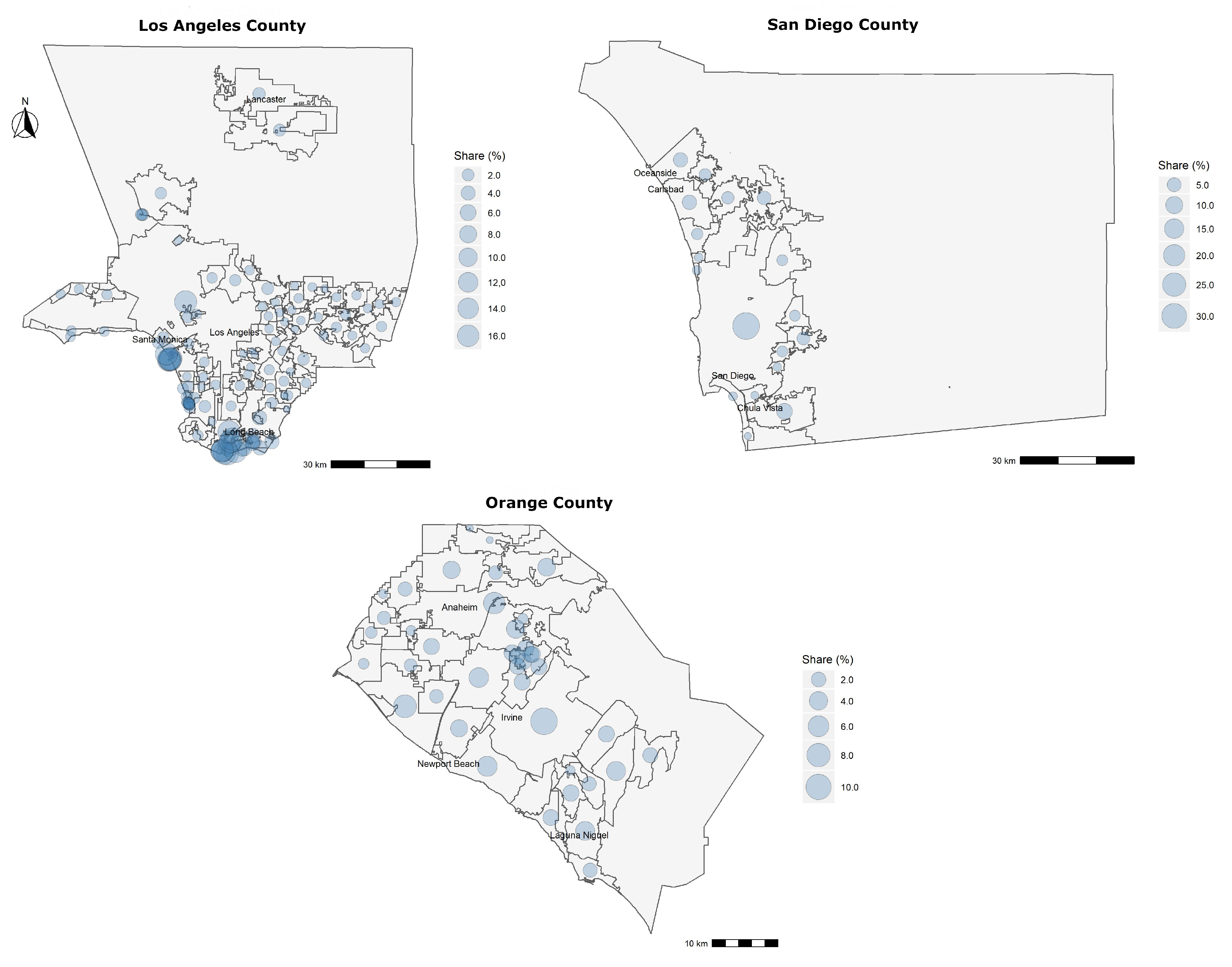Figure 1 shows the share of data for the three counties, on a per city basis. Since the raw dataset consists of appraisal data that are proprietary to CoreLogic^® and contains some private information, we are unable to include it here. However, readers who wish to replicate this study may do so by leveraging data made publicly available through county recorder/appraiser office databases available on the Internet.

Since not every property in a county has been appraised within the 4-year range, we expected to come up with a generalized solution for neighborhood delineation. That is, the estimations should also provide representation for areas not covered by the data. Given that, we first define what a coverage of a subject property is, and how it covers properties that are not present in the data.

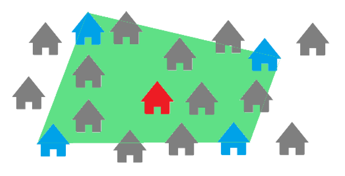
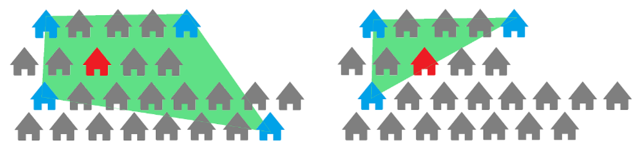
The illustration in Figure 2 represents how we define coverage for a subject property. The subject, highlighted in red, is surrounded by different properties, among which those in blue were chosen as comparable properties during an appraisal, which led to the conclusion that at least the area in green was scoped by the appraiser to find the four comparable properties and is now defined as the coverage of this subject. Through these coverage polygons, we can also find subjects that overlap most and could present similar characteristics.

4. Methodology

4.1. Spatial Filtration

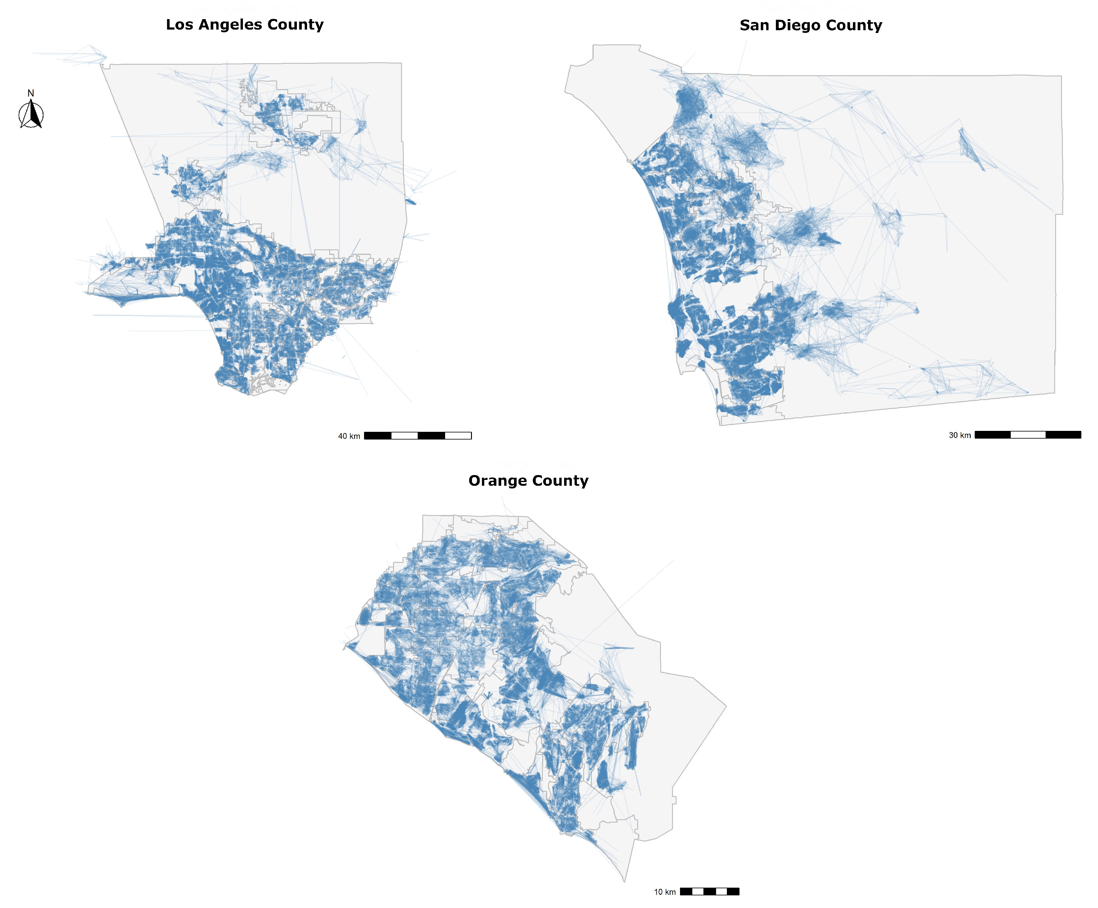
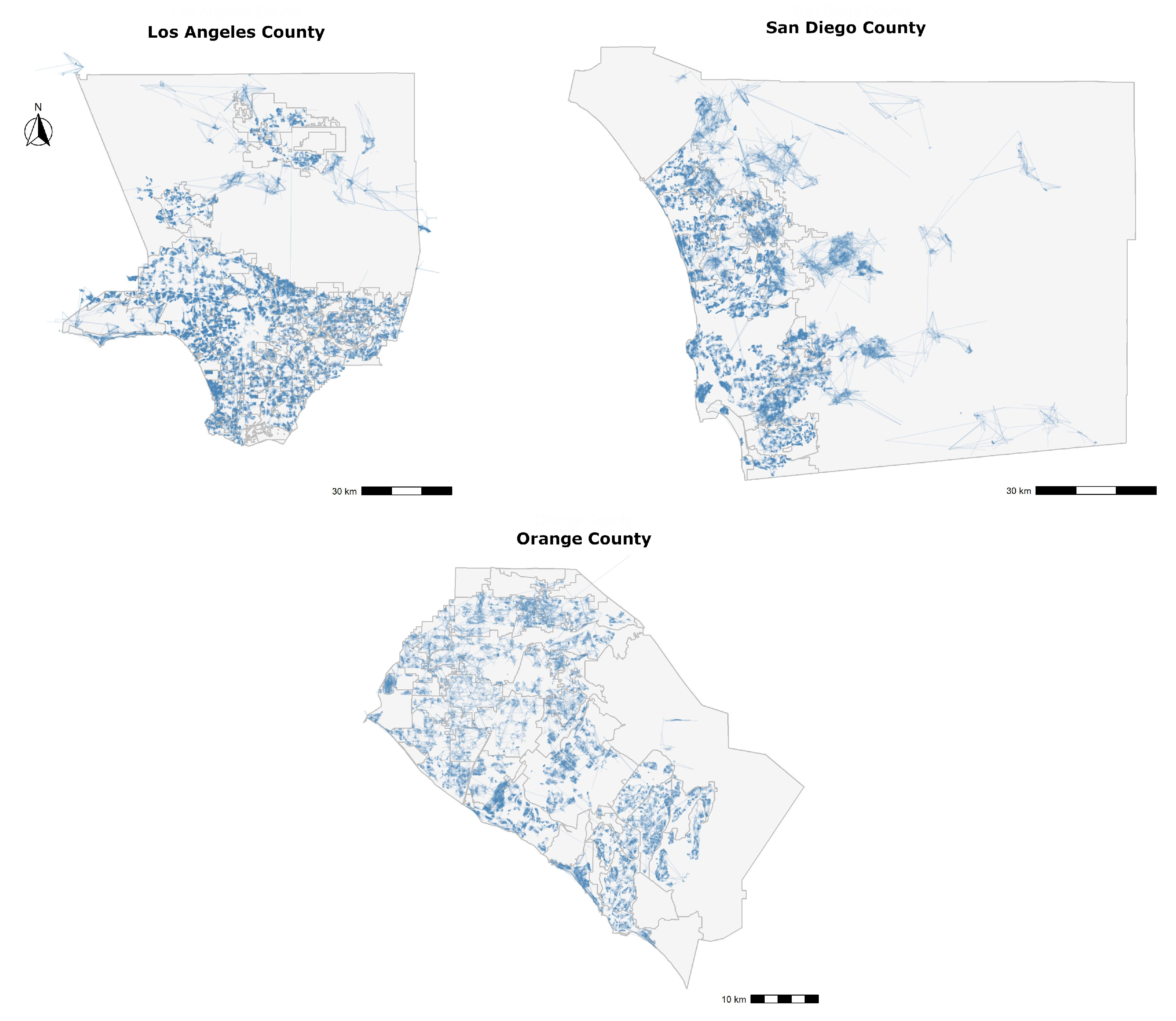
We are interested in generating neighborhoods using the geographical locations of subjects and their comparable properties. As an initial step, we first mapped the current magnitude of that relationship in the data. Figure 3 provides a network map, where each subject is linked to a comparable property using a single line segment. For all 3 counties, there are regions of dense links, especially in urban areas, and the dense regions themselves are separated by small boundary-like regions of little to no links. An overlap of line segments in a small area points to the overlap in the coverage of subjects, and that these subjects share comparable properties, or even that one subject turns out to be a comparable property for another subject. The areas with less links separate the dense network regions from one another to show that the subject coverage overlap between two dense regions is low, and that the appraisers rarely enter the second dense region to find comparable properties for subjects in the first one.

To delineate neighborhoods that represent properties that are similar in characteristics, we need to first reduce the overload of coverage in the dense regions. To do so, we will utilize the distances between subjects and their comparable properties, and use them in a spatial filter, to prune these regions. Once we apply the filters, we can then apply a clustering algorithm to delineate neighborhoods. Demšar et al. [32] detailed applications of principal component analysis (PCA) on spatial data to reduce dimensionality, while Hughes and Haran [33] also discussed getting results by reducing dimensions on non-Gaussian spatial data. Additionally, the iterative self-organizing data analysis technique algorithm (ISODATA) is a popular option for unsupervised segmentation of spatial data, as shown by [34,35], for segmenting remote sensing images. These reduction and segmentation algorithms, however, require a multidimensional feature space and because of their sensitivity to dimensions, exhibit poor speeds when the number of dimensions increase [36].

Our feature space consists of just a distance value between subjects and their comparable properties, and we want to ensure that reduction occurs only on the basis of proximity between properties that are directly involved in an appraisal. Coding this information about which properties were included in an appraisal for which other properties, to apply any of the algorithms discussed earlier, would result in a very large feature space. This feature space would also scale based on how rural or urban the focus region is. To that end, we instead used a set of simple but very fast spatial filters that we describe below. These filters smartly remove comparable properties from the data based on the proximity to their subject properties and not based on their location on a geographical map. Once the coverage is reduced, we use a powerful clustering algorithm, HDBSCAN, to generate neighborhood boundaries.

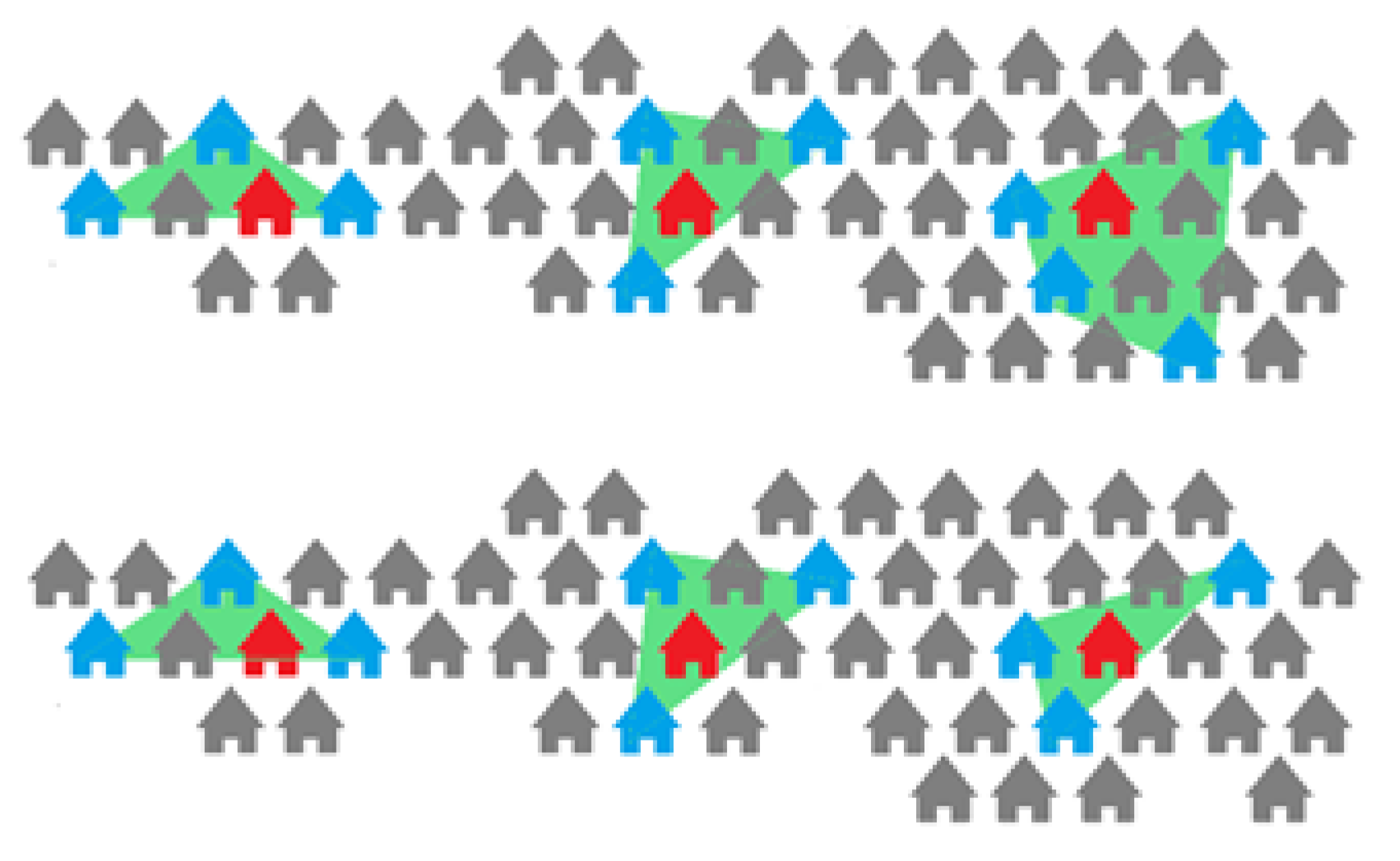
4.1.1. Filter 1

The first filtering algorithm removes all comparable properties from the data that are farther away from their subject property than a set average threshold value for each region. The threshold is based on the geographical location of the region, the size of the coverage of the subject, and the number of comparable properties available for it. Using the geographical coordinates, we are able to filter the data intelligently. Figure 4 illustrates how the coverage for a subject changes before and after the application of this filter.

4.1.2. Filter 2

This filtering algorithm takes advantage of the street address of each subject available in the data. This is a more aggressive form of Filter 1 wherein we now also prune comparable properties if they lie farther than a distance threshold compared to the street segment a subject property is situated on. This filter takes into account how subjects should be perceived if they are packed together. If two subject properties lie on the same street, they are more likely to share similar characteristics, and their individual sets of comparable properties can be thought of being part of a larger pool for that street, which we can then prune to find a more concrete structure for our neighborhood estimations, as seen in Figure 5. The individual filter (Filter 1) is not applied on these subjects, and instead, a street-wise filter is applied to take advantage of the presence of multiple subjects on a street. We add that no matter which filter is applied, the relative positions of subjects and their comparable properties do not change, and the filters maintain the integrity of the inherent relationships between appraised properties.

4.1.3. Filter 3

The only information we have on the streets in a region is by the location of subject properties situated on them. We do not have information about every street in the region, how long it is, how many intersections it passes through, and what its general shape is. These features could be informative in investigating how an appraiser views properties that are across the highway or an avenue, when looking for comparable properties for a subject. This filter applies this knowledge to further prune properties. Using this filter, we remove data for subjects situated along highways or long avenues, as there is a possibility of two subjects being situated on either end of a long street or being connected through a chain of comparable properties. Two densely linked regions that are connected through a series of a handful of comparable properties should not be counted as a single region, and this filter accounts for that. This filter does not affect the coverage structure on either side of a street in question, as seen in Figure 6, and only the bridging subjects and comparable properties are removed.

We present the pseudo-code for the three filters in Algorithm 1. The threshold $\mathit{t}$ is parameterized to ensure that neighborhoods generated for rural and urban regions are scaled accordingly. The mode $\mathit{m}$ is set to true or false based on which filter is being applied.

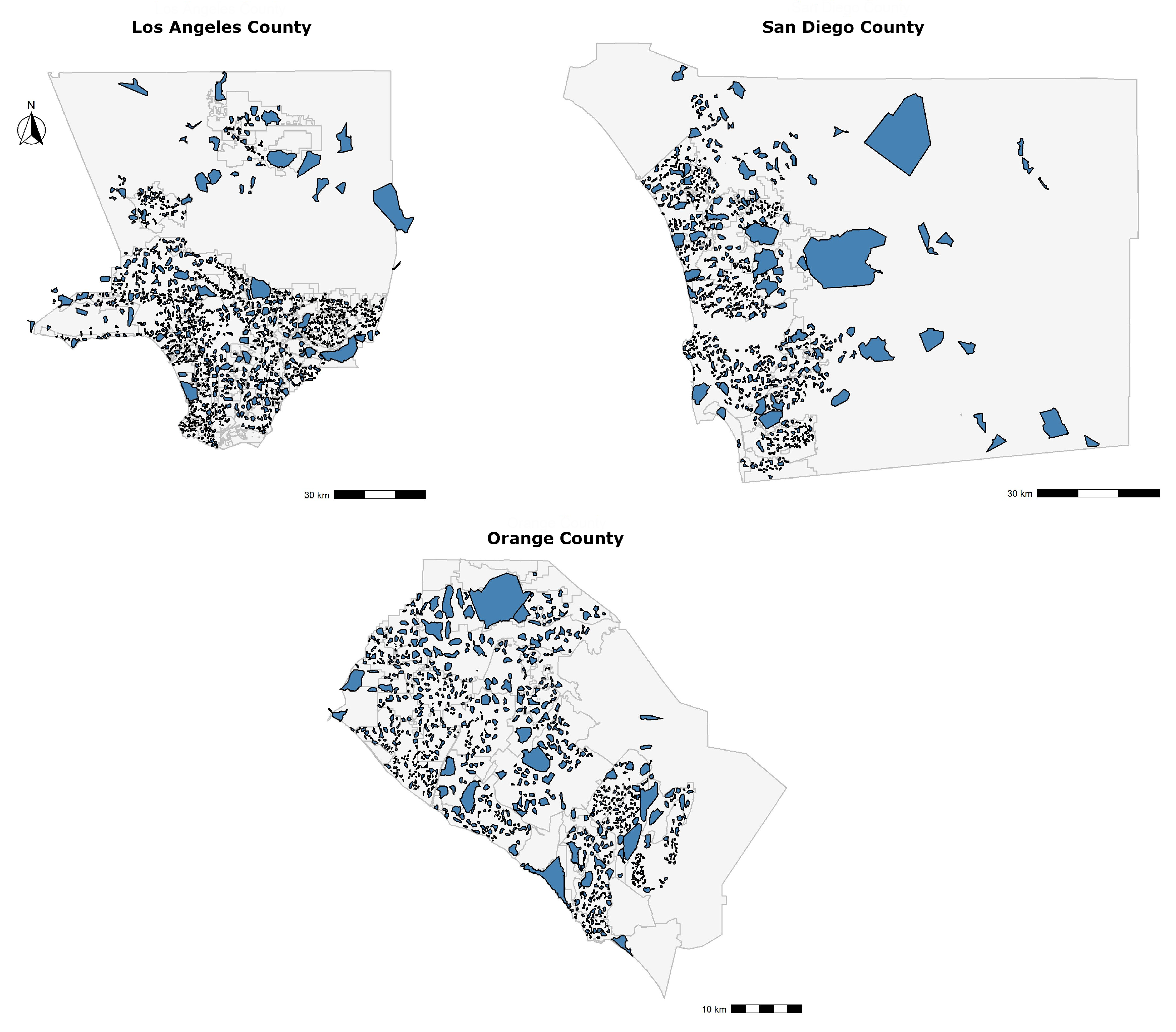
Figure 7 shows the linked map after applying these spatial filters. By comparing it with the unfiltered map, in Figure 3, we note that areas of dense linkages are still present but are now more separable. We term these areas as focus regions of appraisals, as they show most overlap of subjects’ coverage, filtered and extracted from appraisal information, and point to the fact that most of the time, a property selected as comparable for a subject in one of these focus regions is most likely going to be from the same focus region. We will confirm this hypothesis in the Results section.

Algorithm 1: Spatial filter to reduce data set.

4.2. Neighborhood Delineation

Once all filters are applied and a pruned map is found, we can apply a spatial clustering algorithm to separate the dense connectivity regions into separate neighborhoods. Hierarchical density based spatial clustering with an application to noise (HDBSCAN) is an unsupervised machine learning algorithm which uses a hierarchy to extract a flat clustering based on the stability of clusters [37]. These clusters will become our estimated neighborhoods, which are composed of properties that share similar characteristics, through the eyes of an appraiser, and can interchangeably be used as comparable properties for each other.

HDBSCAN also accounts for presence of regions of different densities in the data and is able to allocate some data points as noise, that is, points that do not belong to any cluster and should be removed. The algorithm uses a single parameter, the minimum number of data points required to define a cluster. For each section of the region, we find the optimal value of this parameter through an iterative application of HDBSCAN on the geographical coordinates of all comparable properties. Studies have discussed parameter-free clustering algorithms [38,39], and specifically working with spatial data [40]. However, these applications sacrifice the significance of high or low-density regions in the data. Instead, with an iterative process, we find a parameter that optimizes the balance between the number of clusters and the number of noise points. For each cluster generated, we define its boundary using the concave hull algorithm [41]. Concave hull uses a k-Nearest Neighbors approach to estimate a suitable boundary for a set of points and does not cover maximum area, as a convex hull polygon might do. Since a neighborhood can vary from a set of ten properties on adjacent streets to encompassing an entire small town, a concave hull for the boundary ensures that the true size and shape of a neighborhood is represented.

Figure 8 shows the delineated neighborhoods for the three Southern California counties. We found neighborhoods of different shapes and sizes, consisting of properties ranging from a dozen to several hundreds. We noticed that the size of the neighborhoods increases greatly when the method was applied to rural areas—north of Los Angeles County and west of San Diego County—as properties are more sparsely located, and a larger distance is covered when conducting an appraisal. To answer the first research question, we have used spatial filters and a clustering algorithm, applied only on the geographical distance between subjects and their comparable properties, to estimate neighborhoods. We will discuss the validity of these neighborhoods in the Results section.

Table 1. Running time of algorithm with comparable property count for all counties.

Region	Data Size	Data Size (Post Filtration)	Spatial Filter Runtime (secs)	Spatial Cluster Runtime (secs)
Orange County	332,411	185,391	79.22	114.84
San Diego County	435,653	238,564	106.44	138.03
Los Angles County	802,130	431,123	197.38	291.54

shows the running time of the applied method for all counties. We also show the number of comparable properties before and after the application of the spatial filters. The algorithm was written in the R scripting language [42] and was executed on a 24 core Intel Xeon processor with 264 GB memory. Because there is no time spent on training a model with sample data, as in the case of neural network techniques, or pre-processing the data to apply PCA and other similar algorithms for reduction, the proposed methodology generates neighborhoods quickly and only scales with the sample size.

5. Results

We first compare the generated neighborhoods with ZIP code and Census tract delineation and show which tabulation shows the least variation in property features, as well as show our linear regression done with these tabulations to find which one was the best predictor of property features such as valuation, square footage, sale price, price per square foot, and age. Next, we will show the stability of each neighborhood, from the appraisals’ perspective, and which neighborhoods have grown or shrunk over the years.

To compare the delineated neighborhoods with ZIP codes and Census tracts, we made use of a smaller data set provided, which contains information on the five property characteristics for every subject. We extracted the ZIP code and Census tract information for all properties after estimating the neighborhoods and joined it with the characteristics data to conduct our tests.

5.1. Coefficient of Variation

The sample coefficient of variation ($C_v$) is also defined as the ratio of the standard deviation to the mean of the sample [43]. It describes the dispersion of a variable in a way that it does not depend on the variable’s measurement unit. We use it to compare how each tabulation criteria (estimated neighborhood, ZIP code, Census tract) explains the variation in a property’s characteristics. As we computed the coefficient on a sample, we compared the values of the unbiased estimate of the population coefficient of variation (${\widehat{C}}_v$) instead:

$$C_v=\frac{S}{\overline{x}}$$

(1)

$${\widehat{C}}_v=(1+\frac{1}{4N})C_v$$

(2)

where $C_v$ is the sample coefficient of variation, S is the sample variance, $\overline{x}$ is the sample mean, ${\widehat{C}}_v$ is the unbiased estimate of the population coefficient of variation, and N is the sample size.

For each property feature, we calculated ${\widehat{C}}_v$ for each group in a tabulation and reported the overall average unbiased estimate for each tabulation criterion. Across the three counties, we found that the delineated neighborhoods, generated using the geographical location of appraised properties, provide the smallest ${\widehat{C}}_v$ for each property characteristic, as seen in

Table 2. Average unbiased estimate of coefficient of variation for each tabulation criteria across 3 counties (lower is better).

	Orange County			Los Angeles County			San Diego County
Property Feature	ZIP Codes	Census Tracts	Neighborhoods	ZIP Codes	Census Tracts	Neighborhoods	ZIP Codes	Census Tracts	Neighborhoods
Valuation	0.543	0.513	0.478	0.558	0.516	0.504	0.557	0.512	0.461
Sale Price	0.339	0.265	0.234	0.338	0.283	0.283	0.312	0.263	0.230
Price per ft2	0.200	0.183	0.171	0.258	0.230	0.225	0.207	0.195	0.183
Square Footage	0.348	0.286	0.228	0.368	0.300	0.284	0.356	0.204	0.254
Age	0.181	0.128	0.112	0.321	0.262	0.259	0.265	0.192	0.172

. The smallest ${\widehat{C}}_v$ values for each property feature are highlighted in red. By comparison, a ZIP code is considerably larger than an average neighborhood and a Census tract, so the variation is a sharp decline for the latter two tabulation criteria. The estimated neighborhoods also outperforms the equally sized Census tracts in reducing the variation in property characteristics within them. This result shows that we were able to generate neighborhoods that do in fact contain properties that are similar to each other in characteristics and can be used as comparable properties for subjects in the same neighborhood. The results are also significant, in that they cover three different regions with varying population densities, so our spatial filter, applied with a threshold based on the locations of subject properties, has also worked well. A one way ANOVA [44] showed a significant effect of the tabulation criteria on the unbiased estimates of coefficient of variation, across all property features (p < 0.001). A detailed table with the results of the ANOVA test is presented in Appendix A.

We next fit a series of linear regression models [45] on the sample data to predict each property characteristic, using each tabulation criteria as the predictor for each model, and reported the adjusted R-squared value [46]. The R-squared value, or the coefficient of determination, is a statistical measure of how close the data are to the fitted regression line. It gives the percentage of variation in a variable explained by the predictors. Since we used several hundred delineated neighborhoods and Census tracts as predictors for individual linear regression models, we reported the adjusted R-squared value, which penalizes the coefficient for using too many predictors. Equation (3) gives the formula for adjusted R-squared value:

$$R_{adjusted}^2=1-\frac{(1-R^2)(N-1)}{N-p-1}$$

(3)

where $R_{adjusted}^2$ is the adjusted R-squared value, N is the total sample size, $R^2$ is the R-squared value from the estimated model, and p is the total number of predictors.

Table 3. Adjusted R squared value for each tabulation criterion, with bias and standard error computed by bootstrapping.

Orange County
	ZIP Code			Census Tract			Neighborhood
Property Feature	Adj. R2	Bias	Std. Error	Adj. R2	Bias	Std. Error	Adj. R2	Bias	Std. Error
Valuation	0.391	0.0008	0.0051	0.462	0.0033	0.0054	0.518	0.0068	0.0053
Sale Price	0.515	0.0005	0.0055	0.598	0.0035	0.0056	0.690	0.0058	0.0054
Price per ft2	0.722	0.0016	0.0051	0.740	0.0047	0.0045	0.751	0.0066	0.0046
Square Footage	0.254	0.0010	0.0034	0.416	0.0045	0.0030	0.533	0.0055	0.0040
Age	0.567	0.0009	0.0041	0.663	0.0041	0.0039	0.685	0.0045	0.0037
San Diego County
	ZIP Code			Census Tract			Neighborhood
Property Feature	Adj. R2	Bias	Std. Error	Adj. R2	Bias	Std. Error	Adj. R2	Bias	Std. Error
Valuation	0.456	0.0006	0.0041	0.497	0.0034	0.0040	0.536	0.0044	0.0043
Sale Price	0.566	0.0008	0.0046	0.645	0.0046	0.0037	0.704	0.0042	0.0038
Price Per Sqft.	0.674	0.0012	0.0054	0.693	0.0116	0.0050	0.695	0.0216	0.0048
Square Footage	0.268	0.0014	0.0035	0.436	0.0045	0.0032	0.539	0.0050	0.0040
Age	0.440	0.0048	0.0088	0.647	0.0144	0.0066	0.607	0.0125	0.0084
Los Angeles County
	ZIP Code			Census Tract			Neighborhood
Property Feature	Adj. R2	Bias	Std. Error	Adj. R2	Bias	Std. Error	Adj. R2	Bias	Std. Error
Valuation	0.507	0.0017	0.0029	0.562	0.0058	0.0034	0.552	0.0062	0.0035
Sale Price	0.634	0.0022	0.0033	0.706	0.0059	0.0031	0.687	0.0059	0.0031
Price Per Sqft.	0.740	0.0016	0.0030	0.762	0.0062	0.0027	0.737	0.0059	0.0027
Square Footage	0.313	0.0019	0.0030	0.474	0.0074	0.0029	0.492	0.0069	0.0030
Age	0.428	0.0024	0.0035	0.555	0.0091	0.0031	0.555	0.0067	0.0032

shows the performance of each tabulation criterion as a predictor for a property feature. Highest $R_{adjusted}^2$ values for each property feature are highlighted in red. A linear regression model is able to explain a linear relation between a continuous value and a set of predictors, and a high R-squared value means that the selected predictors are able to explain much variance in the independent continuous value. As an added step, we applied bootstrapping to our linear regression models. Bootstrapping [47] is a non-parametric approach to statistical inference which gives the standard errors and biases of the true coefficients of the model. It works by drawing random samples from the data and by computing statistics on each of those samples. This step adds another level of accuracy to our models. We present the accumulated adjusted R-squared values, their biases, and the standard errors in the table, after resampling from the data 100 times. We show that the delineated neighborhoods outperformed ZIP code and Census tract proxy neighborhoods in Orange and San Diego counties, and were on par with Census tracts in Los Angeles County, with a few exceptions. We also show a table with adjusted R squared values computed by fitting a series of linear regression models without bootstrapping in Appendix B. The results here are significant, not only from a statistical standpoint, but also from the fact that we only used a single feature to produce these neighborhoods. The high performance of our neighborhoods was also not due to the numerical advantage, as there were more Census tracts in Los Angeles county than the number of neighborhoods generated there, and we are presenting the adjusted R squared values, which do account for the number of estimators used in a regression model.

Using these two tests, we answered the second research question we brought forward in this paper. Using the locations of appraised properties, we have not only delineated neighborhoods that contain significantly uniform and similar properties, but that also explain more variation in a property’s features than ZIP code and Census tract proxy neighborhoods.

5.2. Linear Order Subject Pairing

We started our discussion by defining the coverage of a subject, which encompasses properties that are not used in this analysis. As our estimated neighborhoods were built upon the overlap of coverage of different subjects, we wanted to conduct another test to ensure that properties that were clustered into a single neighborhood could in fact be used as comparable with one another. To do so, we tested how closely related the subjects in a neighborhood were, from an appraisal’s point of view. An appraiser can use a single property as a comparable for two or more subjects, during different inspections. A subject in one appraisal can also be a comparable property for another subject. If two subjects are linked via one or more comparable properties, we can estimate how many such subject pairs there are in a single neighborhood. 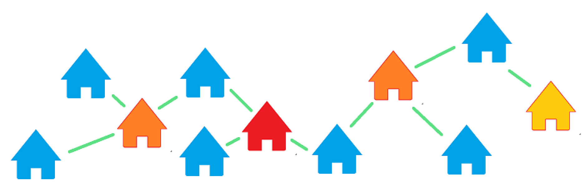Figure 9 illustrates the subject pairs. If all comparable properties are in blue, and we focus on the subject property in red, then the two properties in orange are a first-order pair to the subject in red. That is, they share a single comparable property. The subject property in yellow will then be a 2nd order pair to the subject in red, as the link goes through at least one subject property to chain them together.

A high percentage of first and second-order pairs belonging to the same neighborhood will highlight the fact that these neighborhoods are in fact composed of properties that have been estimated by an appraiser to be similar. We made an effort to use the original, unfiltered data for this analysis. Even though the final delineated neighborhoods are generated using data after the filters are applied, where we removed some comparable and subject properties and pruned the network by a factor, we wanted to ensure that the generated neighborhoods were still able to represent any sample of data, for a new region or location. We present the hit rate, the average percentage of an order pair belonging to the same neighborhood, for the three counties in Southern California.

Table 4. Hit rates of first and second-order pairs of subjects in delineated neighborhoods.

Region	1st Order-Pair Hit Rate	2nd Order-Pair Hit Rate
Orange County	71.2%	61.5%
Los Angeles County	76.6%	64.8%
San Diego County	67.5%	54.2%

shows the hit rate for both first and second order pairs. The high percentages show that more often than not, a first or a second order pair of a subject is found within the same neighborhood that subject belongs to. That is, subjects who are linked with other subjects through one or more comparisons, are more likely to be in the same neighborhood. Given that, properties within a neighborhood can be picked as comparable properties for a subject with much ease and efficiency. This test is an extension to Tobler’s first law, “Everything is related to everything else, but near things are more related than distant things” [48]. Subject pairs are already closely located and so the hit rate percentages should be significantly high, and while we do not discount the significance of spatial autocorrelation, the methodology is a significant improvement over an existing common practice in the industry.

5.3. Yearly Shift

The appraisal data provided by CoreLogic^® contain a sample of appraisals conducted between 2014 and 2018. Now that we have generated definitive boundaries for neighborhoods, and have proven their validity, we now focus on seeing how the neighborhoods grow or shrink over the years. The contention of using Census tracts is that they remain stagnant for 10 years (in the US) and do not change with a market shift. Emergence of a new neighborhood, a sell-off of a set of properties, and even gentrification, will not be considered right away. Given this fact, performing real estate analysis on a Census tract-level will lack validity. A timeseries analysis of property prices in a city or region is quite common in developing an understanding of the real estate market and in predicting the future dips in prices, as used by Quan and Titman [49], and Chiang, Lee, and Wisen [50]. For this analysis, we focus on the shift in the shape of a neighborhood. A delineated neighborhood that constantly grows points to a further growth in the coming years. If we are able to find neighborhoods that have constantly grown or shrunk, across all four years in our range, then we can make a prediction that they will continue to do so in the future.

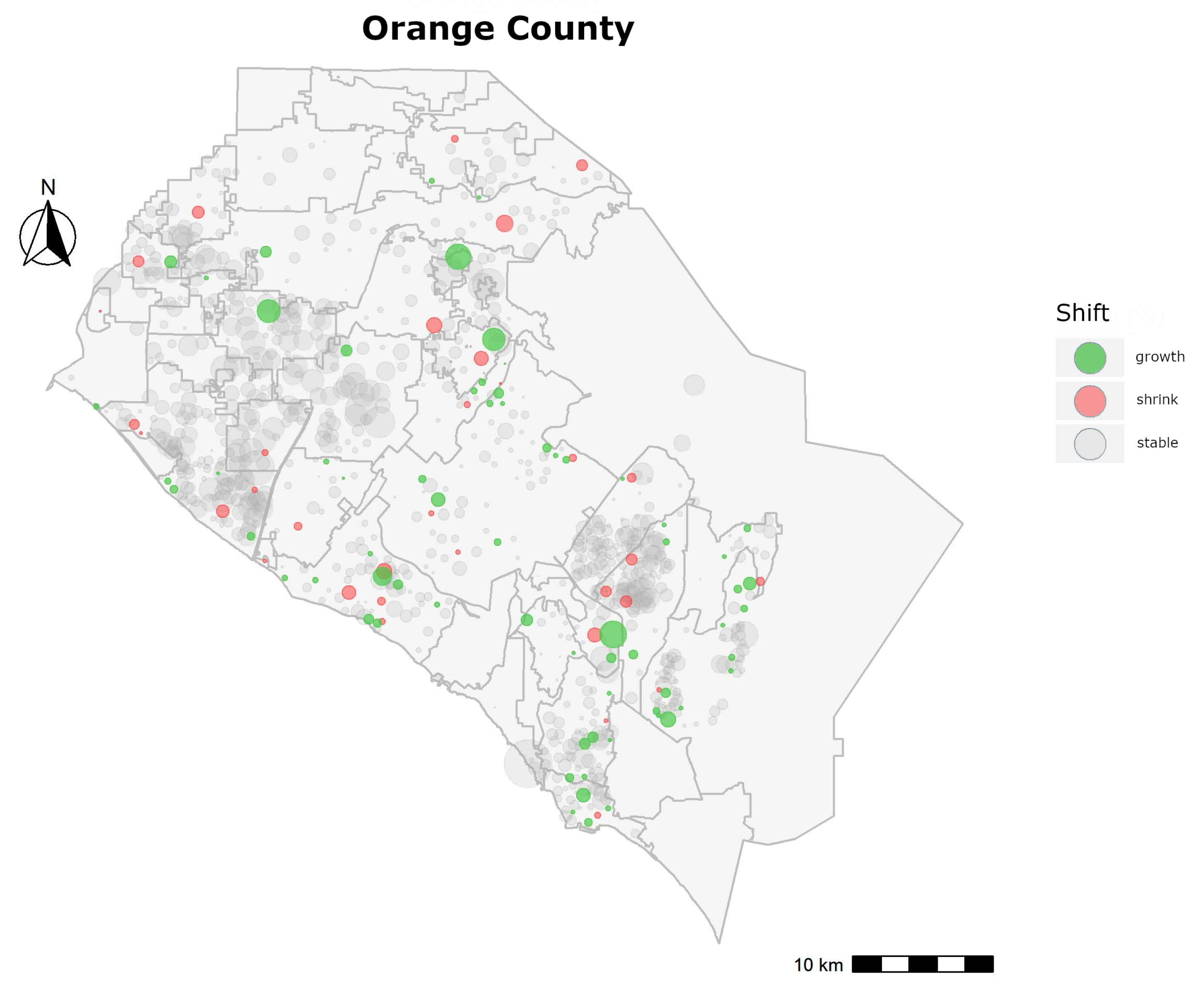
To calculate yearly shift for a neighborhood, we first found the two directions in which most properties lie, relative to the centroid of the neighborhood. This allowed us to focus on the area within a neighborhood that saw the most activity and should be used for any inter-neighborhood analysis. For those directions, we then calculated the average distances between properties and the centroid and evaluated whether the distance was constantly increasing or constantly decreasing, over the years. Our selection criterion was conservative, and we classified a neighborhood to be growing or shrinking only if a neighborhood’s average distance increased or decreased every year. Given the strict setup, we observed that most neighborhoods showed no sign of growth or contraction, as seen in Figure 10. Each circle points to a neighborhood for Orange County and its size is based on the size of the neighborhood. Circles in gray signify neighborhoods with no shift, while those in green point to growth, the ones in red show shrinkage. A steady growth, across all years, alludes to the fact the appraiser now travels farther away to find comparable properties for a subject in the neighborhood and its boundary also needs to change, to potentially cover properties that might be used as comparables in the coming years.

This also affects the real estate market in and around a neighborhood. If the appraiser finds comparable properties beyond the neighborhood boundary of 2014 when conducting appraisals in 2015, it shows that the properties inside the neighborhood are no longer similar in characteristics to the subject property and the inhabitants are making improvements to their houses, which then has the potential of inviting buyers from a more diverse economic background. An area with adjacent neighborhoods with steady growth is a strong indication of a shift in the market and it points to an emerging sub-market with undeveloped land that might become a focus of the real estate market in the coming years.

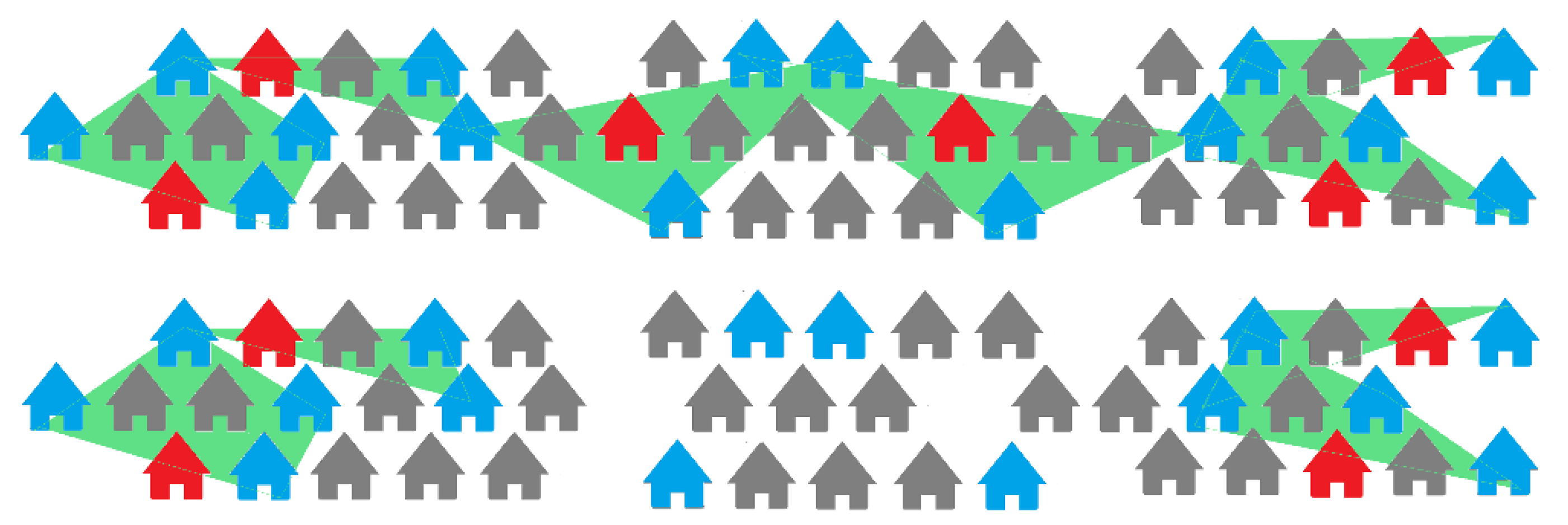
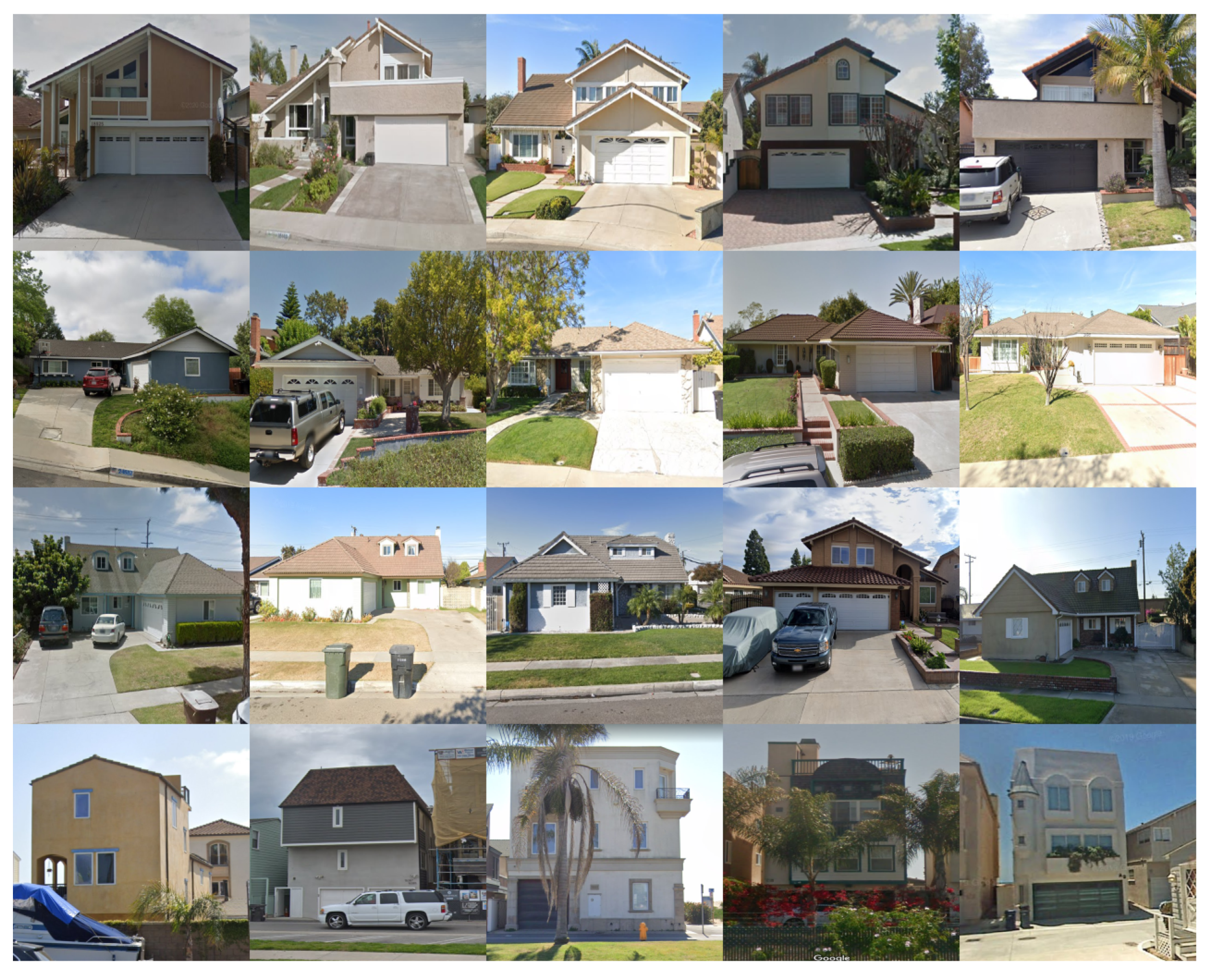
Having the ability to grow with time gives an extra edge to the delineated neighborhoods when compared with the static boundaries of ZIP codes and Census tracts. For future demographic, socioeconomic studies, analyses could be conducted on the level of these neighborhoods, which will provide a more concrete segregation of properties and the inhabitants. Figure 11 shows a sample of properties that were binned into different neighborhoods based on physical features (size and number of stories) and location (beachfront properties for images in the last row).

6. Conclusions

In this paper, we present a novel approach to solving the problem of delineating neighborhoods in a region, that contain properties of similar characteristics, by using the geographical distance between subject and comparable properties, in an appraisal. A limitation of this approach is that the estimated neighborhoods do not cover an entire region. The sample data does not cover appraisals for each individual property, and through the application of spatial filters and a clustering algorithm that deems some properties as noise, we end up with a significant portion of properties that are not within any neighborhood. Our approach, however, uses just the distance between subject and comparable properties to delineate these neighborhoods, and if this approach were to be scaled on a larger level, we would only need the appraisal information to find neighborhoods for new regions, compared to the need to have all characteristic features of properties, had we taken the neural network approach. This limitation, for a future study involving delineating neighborhoods using spatial distance between properties, could be overcome through application of generative algorithms where most significant neighborhoods boundaries are drawn first and are iteratively expanded, until the entire region is covered by delineated neighborhoods. Our algorithm, in essence, is able to connect the knowledge gathered by appraisers through the years, about their specific focus regions, with the market estimations of those regions. Basing our approach on the appraisal data, we highlight the contribution of appraisers to the real estate market and their impact on the observations and predictions we make.

We generate neighborhoods that maintain the relationship between similar properties, highlight an appraiser’s intuition for a region, and have the ability to grow or shrink in the real estate markets. Our neighborhoods are also an improvement on ZIP codes and Census tracts, which are commonly used in demographic and socioeconomic analyses, in predicting property characteristics and explaining their variability.

References

- Sabry, F.; Franceschelli, I.; Claxton, D. Home Equity, Home Value, and Determinants of Mortgage Defaults During the Credit Crisis. J. Real Estate Pract. Educ. 2016, 19, 125–148. [Google Scholar] [CrossRef]
- Forsyth, F. Family Composition and Consumption. J. R. Stat. Soc. Ser. A (Gen.) 1963, 126, 140–141. [Google Scholar] [CrossRef]
- Kish, L.; Lansing, J.B. Response errors in estimating the value of homes. J. Am. Stat. Assoc. 1954, 49, 520–538. [Google Scholar]
- Pagourtzi, E.; Assimakopoulos, V.; Hatzichristos, T.; French, N. Real estate appraisal: A review of valuation methods. J. Prop. Invest. Financ. 2003, 21, 383–401. [Google Scholar] [CrossRef] [Green Version]
- Kain, J.F.; Quigley, J.M. Note on owner’s estimate of housing value. J. Am. Stat. Assoc. 1972, 67, 803–806. [Google Scholar] [CrossRef]
- Diaz, J. An investigation into the impact of previous expert value estimates on appraisal judgment. J. Real Estate Res. 1997, 13, 57–66. [Google Scholar]
- Northcraft, G.B.; Neale, M.A. Experts, amateurs, and real estate: An anchoring-and-adjustment perspective on property pricing decisions. Organ. Behav. Hum. Decis. Process. 1987, 39, 84–97. [Google Scholar] [CrossRef]
- Hernandez, J. Redlining revisited: Mortgage lending patterns in Sacramento 1930–2004. Int. J. Urban Reg. Res. 2009, 33, 291–313. [Google Scholar] [CrossRef] [Green Version]
- Grigg, D. The logic of regional systems. Ann. Assoc. Am. Geogr. 1965, 55, 465–491. [Google Scholar] [CrossRef]
- Bourassa, S.C.; Hamelink, F.; Hoesli, M.; MacGregor, B.D. Defining housing submarkets. J. Hous. Econ. 1999, 8, 160–183. [Google Scholar] [CrossRef]
- Kauko, T. A comparative perspective on urban spatial housing market structure: Some more evidence of local sub-markets based on a neural network classification of Amsterdam. Urban Stud. 2004, 41, 2555–2579. [Google Scholar] [CrossRef]
- Kohonen, T. The self-organizing map. Proc. IEEE 1990, 78, 1464–1480. [Google Scholar] [CrossRef]
- Hipp, J.R.; Faris, R.W.; Boessen, A. Measuring ‘neighborhood’: Constructing network neighborhoods. Soc. Netw. 2012, 34, 128–140. [Google Scholar] [CrossRef] [Green Version]
- McKenzie, G.; Liu, Z.; Hu, Y.; Lee, M. Identifying urban neighborhood names through user-contributed online property listings. ISPRS Int. J. Geo-Inf. 2018, 7, 388. [Google Scholar] [CrossRef] [Green Version]
- Coulton, C.J.; Korbin, J.; Chan, T.; Su, M. Mapping residents’ perceptions of neighborhood boundaries: A methodological note. Am. J. Community Psychol. 2001, 29, 371–383. [Google Scholar] [CrossRef]
- Sun, S.; Manson, S.M. Intraurban migration, neighborhoods, and city structure. Urban Geogr. 2012, 33, 1008–1029. [Google Scholar] [CrossRef]
- Chappell, N.L.; Funk, L.M.; Allan, D. Defining community boundaries in health promotion research. Am. J. Health Promot. 2006, 21, 119–126. [Google Scholar] [CrossRef]
- Spielman, S.E.; Thill, J.C. Social area analysis, data mining, and GIS. Comput. Environ. Urban Syst. 2008, 32, 110–122. [Google Scholar] [CrossRef]
- Arribas-Bel, D.; Nijkamp, P.; Scholten, H. Multidimensional urban sprawl in Europe: A self-organizing map approach. Comput. Environ. Urban Syst. 2011, 35, 263–275. [Google Scholar] [CrossRef] [Green Version]
- Poorthuis, A. How to draw a neighborhood? The potential of big data, regionalization, and community detection for understanding the heterogeneous nature of urban neighborhoods. Geogr. Anal. 2018, 50, 182–203. [Google Scholar] [CrossRef]
- Ratti, C.; Sobolevsky, S.; Calabrese, F.; Andris, C.; Reades, J.; Martino, M.; Claxton, R.; Strogatz, S.H. Redrawing the map of Great Britain from a network of human interactions. PLoS ONE 2010, 5, e14248. [Google Scholar] [CrossRef] [Green Version]
- Cutchin, M.P.; Eschbach, K.; Mair, C.A.; Ju, H.; Goodwin, J.S. The socio-spatial neighborhood estimation method: An approach to operationalizing the neighborhood concept. Health Place 2011, 17, 1113–1121. [Google Scholar] [CrossRef] [PubMed] [Green Version]
- González, M.A.S.; Formoso, C.T. Mass appraisal with genetic fuzzy rule-based systems. Prop. Manag. 2006, 24, 20–30. [Google Scholar]
- Antipov, E.A.; Pokryshevskaya, E.B. Mass appraisal of residential apartments: An application of Random forest for valuation and a CART-based approach for model diagnostics. Expert Syst. Appl. 2012, 39, 1772–1778. [Google Scholar] [CrossRef] [Green Version]
- Elnakat, A.; Gomez, J.D.; Booth, N. A zip code study of socioeconomic, demographic, and household gendered influence on the residential energy sector. Energy Rep. 2016, 2, 21–27. [Google Scholar] [CrossRef] [Green Version]
- Drewnowski, A.; Rehm, C.D.; Solet, D. Disparities in obesity rates: Analysis by ZIP code area. Soc. Sci. Med. 2007, 65, 2458–2463. [Google Scholar] [CrossRef] [Green Version]
- Acevedo-Garcia, D. Zip code-level risk factors for tuberculosis: Neighborhood environment and residential segregation in New Jersey, 1985–1992. Am. J. Public Health 2001, 91, 734. [Google Scholar]
- Grubesic, T.H. Zip codes and spatial analysis: Problems and prospects. Socio-Econ. Plan. Sci. 2008, 42, 129–149. [Google Scholar] [CrossRef]
- Ananat, E.O. The Wrong Side(s) of the Tracks Estimating the Causal Effects of Racial Segregation on City Outcomes; Technical report; National Bureau of Economic Research: Cambridge, MA, USA, 2007. [Google Scholar]
- Kramer, M.R.; Cooper, H.L.; Drews-Botsch, C.D.; Waller, L.A.; Hogue, C.R. Do measures matter? Comparing surface-density-derived and census-tract-derived measures of racial residential segregation. Int. J. Health Geogr. 2010, 9, 29. [Google Scholar] [CrossRef] [Green Version]
- CoreLogic. Available online: https://corelogic.com (accessed on 8 June 2020).
- Demšar, U.; Harris, P.; Brunsdon, C.; Fotheringham, A.S.; McLoone, S. Principal component analysis on spatial data: An overview. Ann. Assoc. Am. Geogr. 2013, 103, 106–128. [Google Scholar] [CrossRef]
- Hughes, J.; Haran, M. Dimension reduction and alleviation of confounding for spatial generalized linear mixed models. J. R. Stat. Soc. Ser. B (Stat. Methodol.) 2013, 75, 139–159. [Google Scholar] [CrossRef] [Green Version]
- Hemalatha, S.; Anouncia, S.M. Unsupervised segmentation of remote sensing images using FD based texture analysis model and ISODATA. Int. J. Ambient. Comput. Intell. (IJACI) 2017, 8, 58–75. [Google Scholar] [CrossRef]
- Melesse, A.M.; Jordan, J.D. A comparison of fuzzy vs. augmented-ISODATA classification algorithms for cloud-shadow discrimination from Landsat images. Photogramm. Eng. Remote Sens. 2002, 68, 905–912. [Google Scholar]
- Memarsadeghi, N.; Mount, D.M.; Netanyahu, N.S.; Le Moigne, J. A fast implementation of the ISODATA clustering algorithm. Int. J. Comput. Geom. Appl. 2007, 17, 71–103. [Google Scholar] [CrossRef]
- McInnes, L.; Healy, J.; Astels, S. hdbscan: Hierarchical density based clustering. J. Open Source Softw. 2017, 2, 205. [Google Scholar] [CrossRef]
- Cesario, E.; Manco, G.; Ortale, R. Top-down parameter-free clustering of high-dimensional categorical data. IEEE Trans. Knowl. Data Eng. 2007, 19, 1607–1624. [Google Scholar] [CrossRef]
- Hou, J.; Gao, H.; Li, X. DSets-DBSCAN: A parameter-free clustering algorithm. IEEE Trans. Image Process. 2016, 25, 3182–3193. [Google Scholar] [CrossRef] [PubMed]
- Anders, K.H.; Sester, M. Parameter-free cluster detection in spatial databases and its application to typification. Int. Arch. Photogramm. Remote Sens. 2000, 33, 75–83. [Google Scholar]
- Moreira, A.; Santos, M.Y. Concave hull: A k-nearest neighbours approach for the computation of the region occupied by a set of points. In Proceedings of the International Conference on Computer Graphics Theory and Applications, Barcelona, Spain, 8–11 March 2007. [Google Scholar]
- R Core Team. R: A Language and Environment for Statistical Computing; R Foundation for Statistical Computing: Vienna, Austria, 2017. [Google Scholar]
- Abdi, H. Coefficient of variation. Encycl. Res. Des. 2010, 1, 169–171. [Google Scholar]
- Stoline, M.R. The status of multiple comparisons: Simultaneous estimation of all pairwise comparisons in one-way ANOVA designs. Am. Stat. 1981, 35, 134–141. [Google Scholar]
- Kutner, M.H.; Nachtsheim, C.J.; Neter, J.; Li, W. Applied Linear Statistical Models; McGraw-Hill Irwin: New York, NY, USA 2005; Volume 5. [Google Scholar]
- Miles, J. R squared, adjusted R squared. In Wiley StatsRef: Statistics Reference Online; John Wiley & Sons, Ltd.: Hoboken, NJ, USA, 2014. [Google Scholar]
- Freedman, D.A. Bootstrapping regression models. Ann. Stat. 1981, 9, 1218–1228. [Google Scholar] [CrossRef]
- Tobler, W.R. A computer movie simulating urban growth in the Detroit region. Econ. Geogr. 1970, 46, 234–240. [Google Scholar] [CrossRef]
- Quan, D.C.; Titman, S. Do real estate prices and stock prices move together? An international analysis. Real Estate Econ. 1999, 27, 183–207. [Google Scholar] [CrossRef]
- Chiang, K.C.; Lee, M.L.; Wisen, C.H. On the time-series properties of real estate investment trust betas. Real Estate Econ. 2005, 33, 381–396. [Google Scholar] [CrossRef]
© 2020 by the authors. Licensee MDPI, Basel, Switzerland. This article is an open access article distributed under the terms and conditions of the Creative Commons Attribution (CC BY) license (http://creativecommons.org/licenses/by/4.0/).