GIS-Based Mapping of Seismic Parameters for the Pyrenees


1
Department of Graphic Engineering, University of Seville, 41092 Seville, Spain
2
National Geographic Institute of Spain, Andalusia Division, 41013 Seville, Spain
3
Geographic Information System Group, Department of Business and IT, University of Southeast Norway, Gulbringvegen 36, N-3800 Bø i Telemark, Norway
*
Author to whom correspondence should be addressed.
ISPRS Int. J. Geo-Inf. 2020, 9(7), 452; https://0-doi-org.brum.beds.ac.uk/10.3390/ijgi9070452
Submission received: 11 June 2020
/
Revised: 3 July 2020
/
Accepted: 15 July 2020
/
Published: 17 July 2020
(This article belongs to the Special Issue Geo-Informatics in Resource Management)
Abstract
:In the present paper, three of the main seismic parameters, maximum magnitude -Mmax, b-value, and annual rate -AR, have been studied for the Pyrenees range in southwest Europe by a Geographic Information System (GIS). The main aim of this work is to calculate, represent continuously, and analyze some of the most crucial seismic indicators for this belt. To this end, an updated and homogenized Poissonian earthquake catalog has been generated, where the National Geographic Institute of Spain earthquake catalog has been considered as a starting point. Herein, the details about the catalog compilation, the magnitude homogenization, the declustering of the catalog, and the analysis of the completeness, are exposed. When the catalog has been produced, a GIS tool has been used to drive the parameters’ calculations and representations properly. Different grids (0.5 × 0.5° and 1 × 1°) have been created to depict a continuous map of these parameters. The b-value and AR have been obtained that take into account different pairs of magnitude–year of completeness. Mmax has been discretely obtained (by cells). The analysis of the results shows that the Central Pyrenees (mainly from Arudy to Bagnères de Bigorre) present the most pronounced seismicity in the range.
1. Introduction
In seismicity studies, some parameters have a particularly important role. Among others, these are the maximum magnitude (recorded, possible, expected), the b-value of the Gutenberg–Richter (GR) frequency-magnitude (FMD) relation, and a parameter related to the seismic activity (mean seismic activity rate or the a-value of GR) [1,2,3,4,5,6,7,8,9,10,11,12,13]. Some of these studies are based on seismic zonations [1,2], and others are found in a purely geographical grid division [7,11,14,15]. In both cases, the usage of a system capable of adequately integrating different sources of geographic data is advisable. Thus, a Geographic Information System (GIS) can provide the rigor, flexibility, and the power to calculate, show, and analyze the parameters. This fact has been demonstrated previously for natural hazards works [7,16,17,18,19].
Upon Gutenberg and Ritcher [20], the GR relation establishes that the number of earthquakes, N, with magnitude larger than or equal to a given magnitude M (cut-off magnitude), can be expressed as
where a-value estimates the seismic productivity, whereas the slope (known as b-value) measures the size–distribution parameter. The latter expresses the relationship between small and large events. It is usually considered as the essential seismic parameter, which varies from 0.6 to 1.5 for global seismicity [21]. Values between 0.9 and 1.0 can be established as normal b-value [22,23,24]. In many cases, the b-value is considered as a stress-meter, where the higher its value is, the lower the stress is held [25,26,27]. However, other studies [23,28] state that its value must be 1.0, and any variation is due to some issues such as improper calculation, insufficient data, or inhomogeneous detection network.
The main aim of this work is to calculate, represent continuously, and analyze some of the most crucial seismic indicators for the Pyrenees range. Previously, an updated, homogeneous, and extensive catalog has been generated.
The importance of earthquake catalogs in seismic studies is crucial [8,10,11,29,30,31]. Due to the different content of seismic information for both historical and instrumental epochs, a critical point in the catalog analysis is to generate a reliable, updated, extensive, and homogeneous catalog for the studied region to make the results comparable. In areas where historical seismicity data are available, they must be included in the working catalog to conduct a complete and robust analysis [1,2,3,10,32,33,34]. Besides, the size of the (non-small) earthquakes is usually given in moment magnitude (Mw) [35], as it has a direct relation with the released energy through scalar seismic moments and does not get saturated for larger events. To this end, both global and regional parameters can be found in the literature to convert both intensities and different magnitude types into Mw [35,36,37]. Currently, the evolution and improvement of the seismic networks allows for dealing with a considerable amount of data with very high precision in both location and magnitude.
In this work, after preparing the working catalog, the information has been integrated into a GIS. The calculations and representations have been carried out in its environment as it offers some remarkable advantages, such as combining alphanumeric and geographic information or generating high-quality maps.
2. Study Area
2.1. Geological Settings
The Pyrenees is a range of mountains located in the France–Spain border, which spans 450 km long (E–W) and 150 km wide (N–S) [27]. It was formed from the convergence between the Eurasian (to the north) and Iberian (to the south) plates. It happened after an extensive period related to the opening of the Bay of Biscay in the Lower Cretaceous [38,39,40]. Nowadays, the Iberian Peninsula is located in the southwest of the Eurasian plate, which presents a collision movement with the African plate with an estimated rate of between 2 and 5 mm/year in the NW–SE to WNW–ESE direction [2]. Currently, this rate is considerably lower for the Pyrenees [41], despite being the second most seismically active area in the Iberian Peninsula after the Betics.
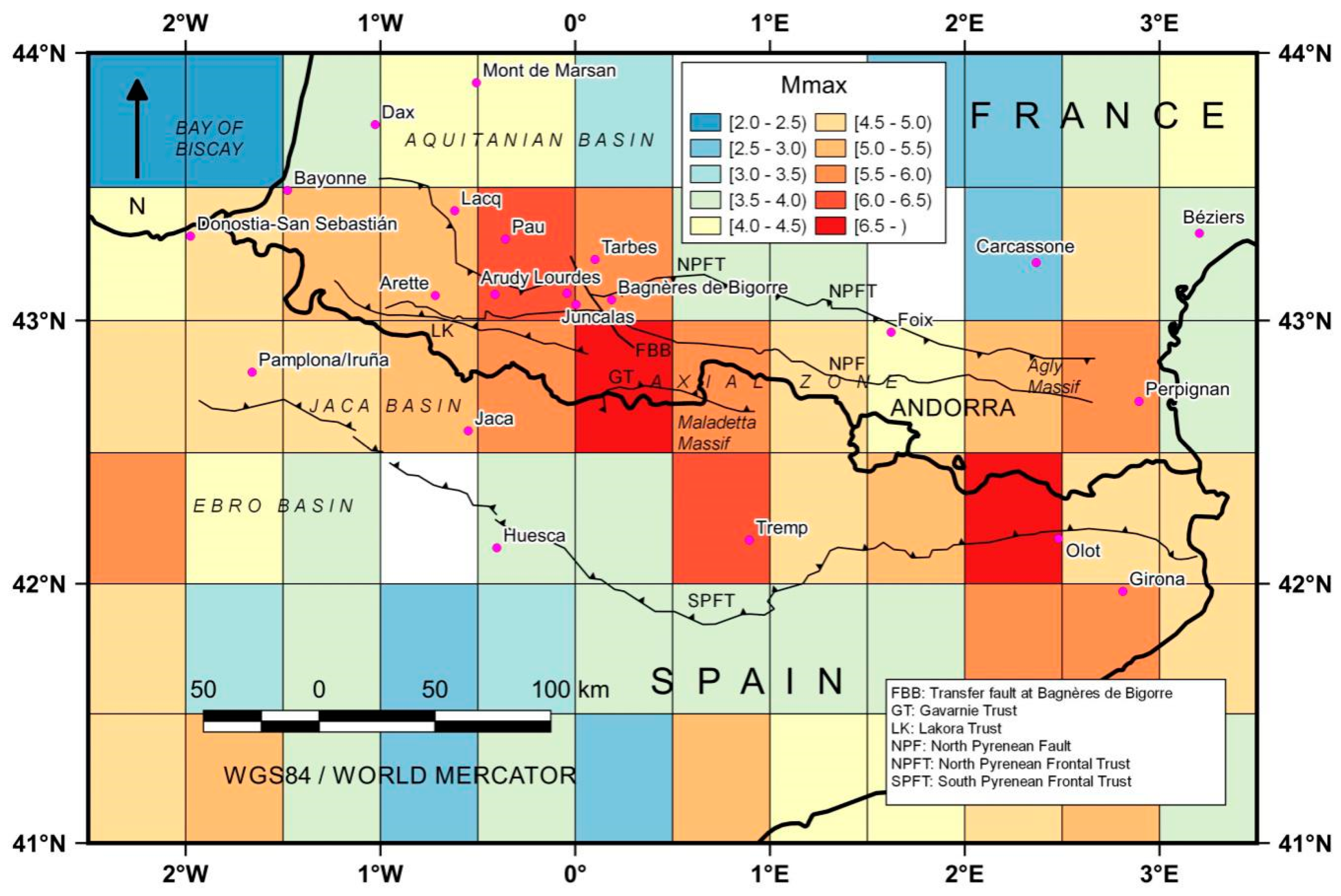
A general view of this belt’s geological structure can be found in [39,42,43,44,45]. Figure 1 presents a general sketch of the geological context.
The main units can be summarized as follows [39]:
- The North Pyrenean Zone (NPZ), which was mainly formed by Mesozoic (Cretaceous) deposits, rides northward over the Aquitaine basin along with the North Pyrenean Frontal Trust (NPFT). The NPZ contains Paleozoic outcrops.
- The Paleozoic Axial Zone, which is located at the central part and presents the highest peaks of the Pyrenees, is composed of Hercynian structures that were reactivated during the Alpine orogeny.
- The South Pyrenean Zone (SPZ), which slid southward down from the Axial zone when it rose, presents Mesozoic (Cretaceous) and Cenozoic (Oligocene) sediments in its composition.
Besides, the so-called North Pyrenean Fault (NPF) is a major east–west tectonic suture, which separates the Axial Zone of the NPZ. This fault is frequently considered as the limit between the Iberian and Eurasian plates. It coincides with an important vertical shift of the Moho discontinuity, where the Iberian side presents a thicker crust.
2.2. Seismicity
The spatial distribution of earthquakes in this belt is complex with different mechanisms, such as denudation, and gravitational collapse, or lithospheric flexure [43]. Therefore, it is necessary to study it carefully when performing a Probabilistic Seismic Hazard Analysis (PSHA). Although the Pyrenees seismicity can be considered as low to moderate; however, some shocks still produced significant damages in the historical period, especially with events either with magnitudes exceeding 6 (M6+), or MSK intensities equal to or larger than VIII [41,46]. For example, on the Spain side, the 1373 earthquake (Io = VIII-IX) occurred in the Ribagorça County (by Maladetta Massif) in the south part of the Central Pyrenees [47]; the Catalan seismic crisis during 1427 and 1428 reached Io = IX, destroyed Olot and Queralbs and caused more than 1000 fatalities [47,48,49]. On the France side, the 1660 Bigorre Earthquake (Io = IX), near Lourdes in the Central Pyrenees [46,50,51], and more recently, the 1750 Juncalas (Io = VIII) in a nearby area [41]. Besides, in the instrumental period, some strong earthquakes have occurred. Among others, 1967 Arette (M5.3) [46,51], in the Atlantic Pyrenees, with Io = VIII, or others in the eastern Pyrenees, in the Agly Massif, such as St-Paul de Fenouillet (M5.0) in 1996 [39,52].
The seismicity takes part mainly in the western part of the NPZ, while in the east, it is lower and more dispersed. Regarding the focal depth, it has to be pointed out that it is shallow, mainly less than 20 km. Besides, the seismogenic crust could correspond to the first 15–20 km of the crust [49].
2.3. Related Works on the Pyrenees Seismicity
Various studies have explored the variation in the b-value in the Pyrenees. Gallart et al. [54] analyzed it for the Arette–Arudy region in the western Pyrenees. Kijke-Kassala et al. [38] calculated the b-value from a regionalization (nine zones). In other works, the Arudy region was analyzed by Sylvander et al. [55], whereas Secanell et al. [56] conducted a PSHA, where they calculated the b-value. Afterward, Secanell et al. [57] divided the Pyrenees into ten seismogenic zones from the ISARD project earthquake catalog and tectonic models, and then b-values were obtained. In addition, in the frame of the PSHA models for Spain and their analysis, some studies have been addressed [1,2,6]. In recent research, Amaro-Mellado et al. [7] produced a continuous b-value map for the whole Iberian Peninsula and adjacent areas; however, an in-depth specific study for the Pyrenees has not been conducted. Rigo et al. [27] analyzed the b-value variation with the depth relating to the differential stress, considering only b-values from a seismic zonation proposed by Rigo et al. [58]. Nevertheless, to the best of our knowledge, no continuous map has been deployed for this specific region, taking into account its seismic circumstances.
3. Data and Methods
In this section, the input data and the methodology conducted to produce the maps of the seismic parameters are described.
3.1. Catalog generation
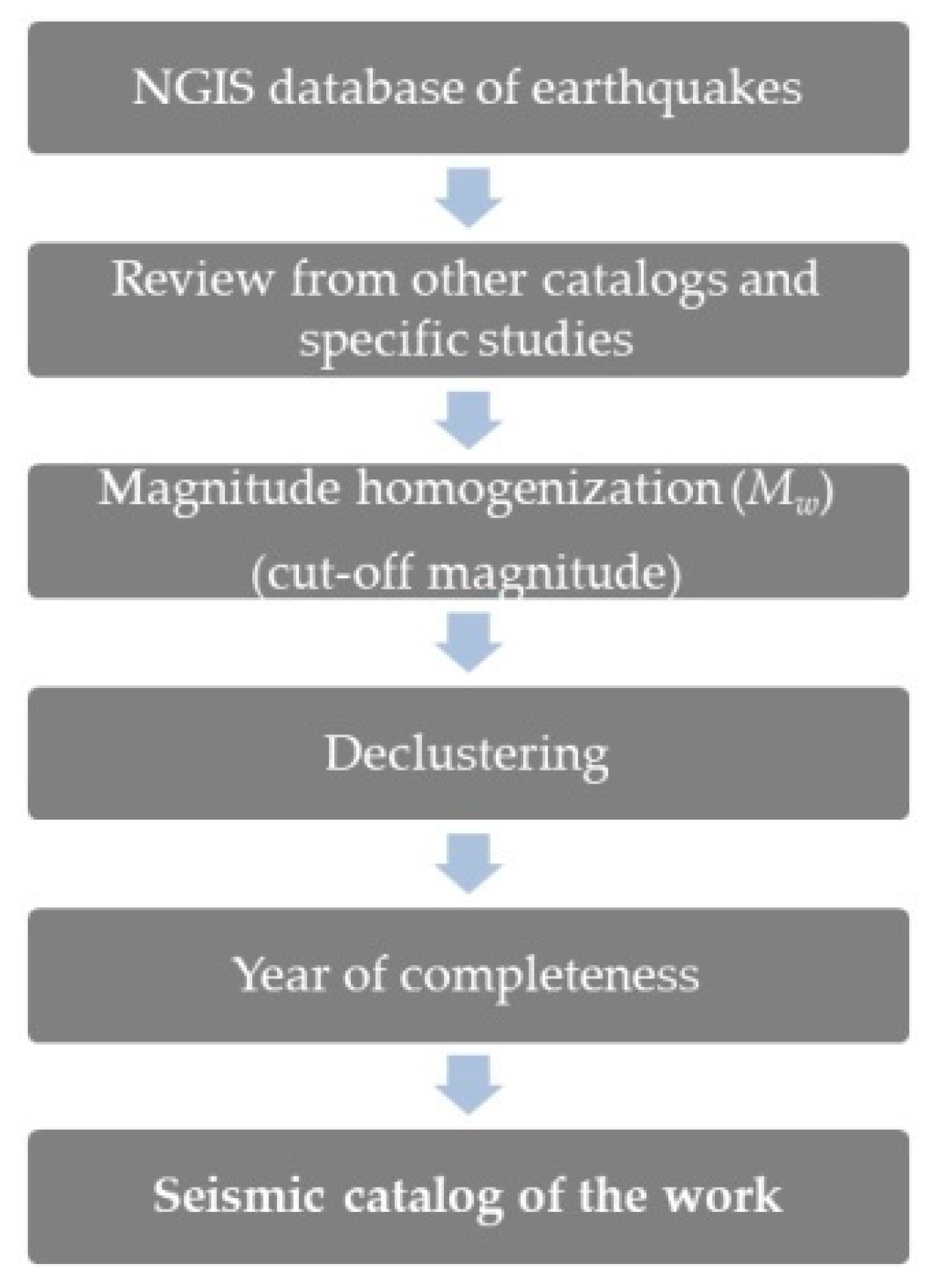
As has been pointed out above, the importance of working with a high quality and reliable catalog is a key issue. The steps required to this end are shown in Figure 2.
3.1.1. The National Geographic Institute of Spain Earthquake Catalog
The earthquake catalog employed in this work takes as a starting point the earthquake catalog of the National Geographic Institute of Spain (hereinafter, NGIS), which can be downloaded from [59]. It has more than 135,000 events between 1373 and the end of 2019, corresponding to the Iberian Peninsula and the Canary Islands and their adjacent areas. Through the years, the sizes of the events have been recorded in different ways (macroseismic intensity or several magnitude types, as will be shown later). The fields recorded in the database include elements such as an ID, date, hour, 3D location, intensity, magnitude, or magnitude type. A detailed study of the NGIS catalog can be found in González [60], where the seismic network evolution is shown.
Regarding the precision in earthquakes’ location, for the whole catalog, shocks from 1997 have a better location than 3 km (4 km in 1985; 7 km in 1983–1984, and it is worse for previous events) [60], but, in regions like the Pyrenees, they are lower thanks to the data contributed to the catalog by other networks [43,60]. Currently, this precision is significatly better, as can be checked in [59].
For this work, the geographical extent considered has been limited by 41° N and 44° N parallels and 2.5° W and 3.5° E meridians. The earthquake distribution of the 24,282 resulting events is shown in Figure 3, where 248 (mostly aftershocks from pre-instrumental and historical periods) have no size assigned.
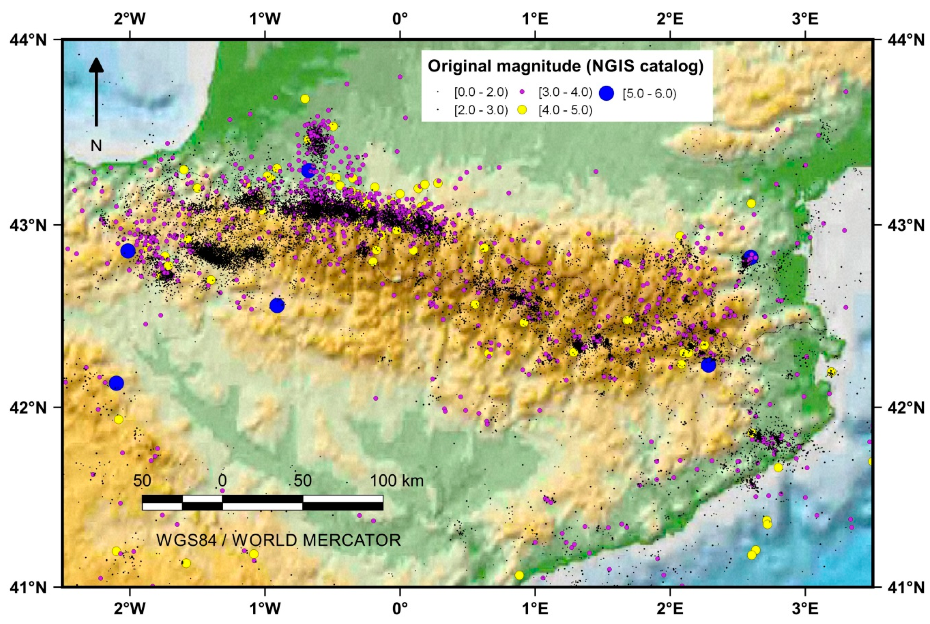
Additionally, for the instrumental period, a map showing the originally recorded magnitudes in the NGIS catalog is presented in Figure 4.
3.1.2. Review from Other Catalogs and Specific Studies
The seismic catalog must be improved with data from other sources, such as from other catalogs or from specific publications (mainly, journal papers) where individual events have been re-evaluated, as has been conducted in similar works such as in [2,6]. Therefore, a thorough revision has been developed, and the size of 31 events has been reviewed, particularly to assign a reliable Mw to the largest events. Special mention is deserved for some earthquakes with a marine epicenter, and with only macroseismic information. Their intensities recorded in the catalog could not be the epicentral ones, due to attenuation, and should be revised. The works that have supported the review are found in [6,39,46,47,49,50,52,55,61,62,63,64,65,66,67].
3.1.3. Magnitude Homogenization and Cut-off Magnitude
Over time, the size of the earthquakes has been calculated in line with the evolution of the seismic network. Besides, it has been stored in different ways in the NGIS catalog, for historical, pre-instrumental, and instrumental periods. It can be found in [2], and it is summarized here (with its uncertainty):
- Epicentral or maximum intensity (until 1923) (0.5 ≤ σ ≤ 1.5).
- Pre-instrumental 1924–February 1962: Duration magnitude [68], mD(MMS) (σ = 0.4).
- March 1962–February 1998: Surface–wave magnitude [68], mbLg(MMS) (σ = 0.3) (<1985); (σ = 0.2) (>1985).
- March 1998–2002: Body–wave magnitude [69], mb(VC) (σ = 0.2) and mbLg(MMS) (σ = 0.2).
- March 2002–onward: Surface–wave magnitude [70], mbLg(L) (σ = 0.2) or mb(VC) (σ = 0.2), or, for the most significant events, Mw (σ = 0.1).
To work with a homogeneous catalog, all the events must possess the same kind of magnitude, and the preferred scale has been Mw for the advantages mentioned earlier. Different authors have proposed global and regional parameters to convert the original size into Mw [35,36,37,71,72,73,74]. Given that both independent and dependent variables have errors, a reduced major axis (RMA) is currently preferred to a least-square ordinary regression [36,71]. In this work, the conversion from the original size of every event to Mw has been conducted from the parameters suggested by Cabañas et al. [36], as they are specific for the Iberian Peninsula and adjacent areas.
After those conversions, a proper b-value requires estimating the magnitude of completeness (Mc), which is an essential and mandatory step to conduct a seismic analysis. Mc can be defined as the lowest magnitude at which 100% of the earthquakes in a space–time volume are detected [10,75]. There are multiple methods to estimate this value, and in-depth analysis can be found in Mignan and Woessner [75].
The method employed in this paper is based on the earthquake catalog, and consists of plotting the non-cumulative FMD in addition to the standard (cumulative) FMD. Assuming self-similarity, Mc is simply the magnitude increment at which the FMD departs from the linear trend in the log–lin plot [75]. The estimate of Mc can be assessed from Figure 5 at 1.8 (Mc = 1.8).
After determining the Mc, regarding the b-value calculation, the cut-off magnitude (Mco ≥ Mc) for this work has been set as 2.0 (M2), to have a margin and, besides, consider a standard value.
3.1.4. Declustering
Although the studies of the aftershocks are necessary to some applications [76,77], the computation of the PSHA is mainly based on a Poisson distribution. Herein, these events must be independent; thus, foreshocks, aftershocks, and seismic swarms must be deleted. Consequently, the resulting catalog contains mainshocks only. This is a tricky process, known as declustering, where two principal methodologies, proposed by [78,79], used to be applied, and a thorough study on it can be found in [80]. In this work, the method suggested by Gardner and Knopoff [78] was selected due to its clarity, simplicity, and stability [2,3,32]. Besides, this method has proven its efficiency in most of the recent research [8,10,31,81,82], and particularly for the studied area [2,7]. As the more energetic an earthquake is, the more temporal and geographical extension is involved, this method defines temporal and spatial windows depending on the main earthquake. There are different values to establish these windows. In this research, the proposal by Uhrhammer [83] has been chosen as it is a conservative solution and widely used [29,81,82,84,85].
The results of declustering, conducted by the ZMAP application [86], show that there are 1434 clusters, whose seismic moment released is about 4.4% of the total seismic moment of the catalog. Finally, 19,625 events remain in the declustered catalog.
3.1.5. Year of Completeness
The NGIS catalog spans more than 600 years in its records, and this study has taken advantage of this sizeable temporal extent. As has been pointed out, the magnitude of completeness must be related to a reference date, due to the seismic network heterogeneities and evolution, and it is crucial to estimate a b-value properly. The larger an event is, the more likely it is to be recorded in distant times.
The best method to calculate the different Mc–year of completeness pairs is a much-discussed subject. In this research, the cumulative method [87,88,89] has been used to estimate the completeness periods for different levels of magnitude, as in other recent works [10,81]. Thus, plotting the cumulative number of earthquakes and time, the year of completeness can be estimated. The catalog is considered complete for a threshold magnitude concerning the time where there is approximately a straight line of the plotted date, so the completeness period varies with time [10]. In this study, the year of completeness has been determined for M2, M3, M4, and M5, as can be seen in Figure 6.
3.1.6. Seismic Catalog of the Work
After all the steps described previously, the events deeper than 65 km have been removed, as they are not relevant for seismic hazard in the area [2].
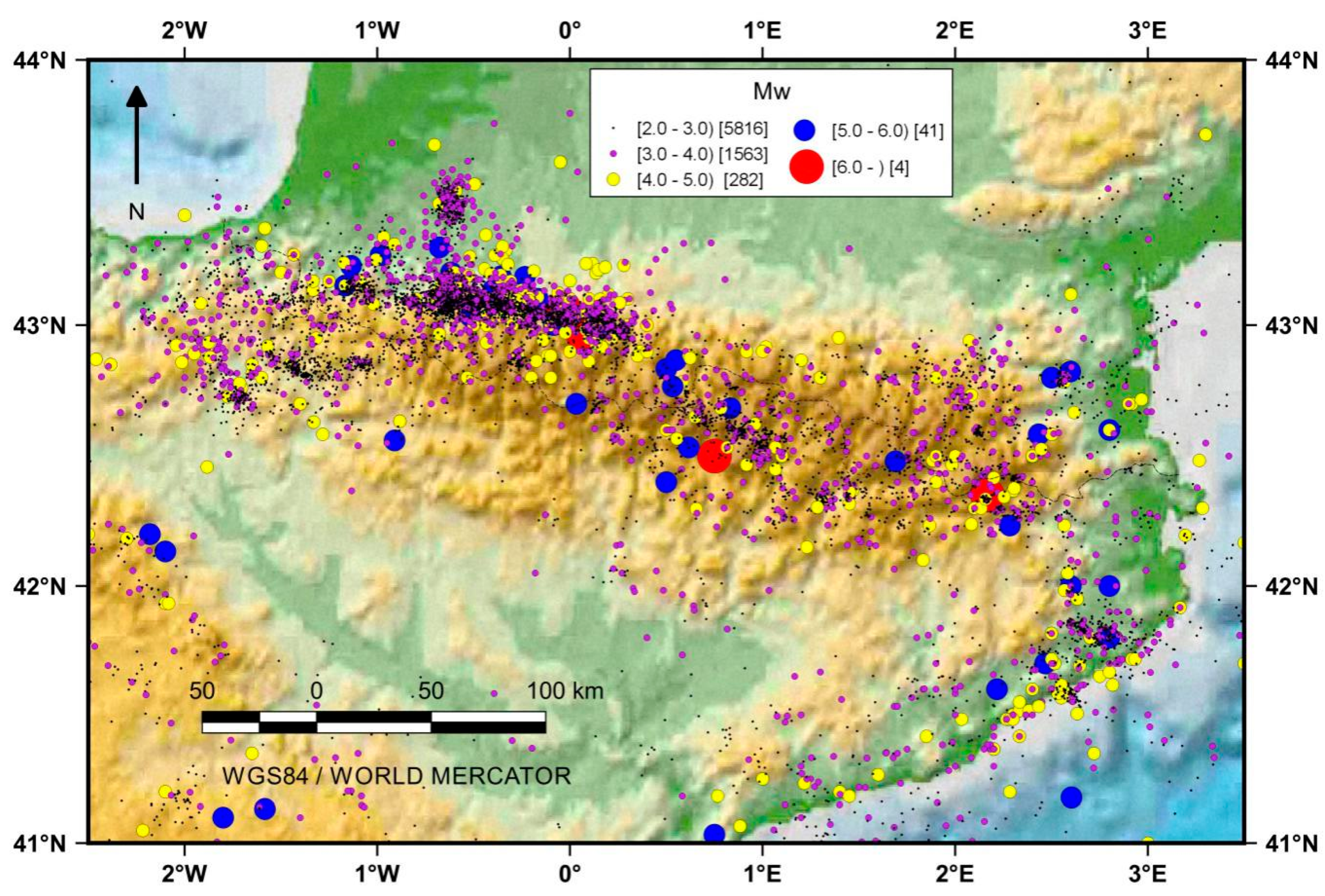
The final catalog consists of 7706 events with Mw from 1373 to 2019 is shown in Figure 7.
3.2. Seismic Parameters
In this subsection, several relevant seismic parameters will be introduced as they are indicators of the seismicity of an area. These parameters are the maximum magnitude, the b-value, and the normalized annual rate for events exceeding M3.
3.2.1. The Maximum Magnitude
The maximum magnitude (Mmax) is closely related to the seismic hazard for an area. Therefore, to appreciate its distribution, a 0.5 × 0.5° grid has been deployed using a GIS tool and covering the whole working area, in a GIS environment. There are different concepts related to the maximum magnitude, such as the largest recorded event, a-value/b-value, the largest physically possible. Besides, there are different approaches (parametric, non-parametric) to calculate its value. Thorough works can be found in [90,91]. In this work, as the temporal extent of the catalog is long, the maximum magnitude of the working catalog for every grid’s cell has been chosen, being aware of the limitations.
3.2.2. The b-value
The b-value is the parameter most studied in seismology and corresponds to the slope of the FMD in a log–log plot. The majority of the authors stated its relationship with the physics of the studied area. It has been deeply studied and is usually analyzed in PSHA works, in prediction, in locating asperities, periodical tidal loading, and energetic characterization [4,8,11,16,25,92,93,94,95].
Although firstly, the least square solution was usually employed to calculate its value, currently, there is a consensus in considering the Maximum-Likelihood-Estimate (MLE) as the best approach to obtain it. This is due to the fact that it does not present interdependency between variables [2]. Over time, a considerable amount of different methods have been suggested for its calculations, such as those found in [13,96,97,98,99,100]. One of the most employed formulae for MLE was proposed by [98,99] for binned data.
where Mc is the cut-off magnitude, is the average magnitude of the earthquakes whose magnitude is larger than or equal to Mc, and ΔM is the binning interval of the magnitude.
In this research, the bin interval is 0.1. The solution proposed by Kijko and Smit [13], through the exposed MLE expression, has been applied. It permits taking into account a longer temporal extent and different magnitude–year of completeness pairs. Moreover, it is said to be simple, manageable, and it is not based on iterations [13].
The method suggested by Kijko and Smit [13] is based on dividing the catalog into more coherent s sub-catalogs, each of a different level of completeness, and with its corresponding year of completeness. It is particularly indicated for incomplete or inhomogeneous catalogs. For every sub-catalog, the MLE proposed by [98,99] is used. Later, b-value is estimated as a weighted solution as:
where bi is the b-value of each of the s sub-catalogs, ni is the sample size of the sub-catalogs, and n is the total number of events considered (n = n1 + n2 + …+ ns).
Each sub-catalog has a known but different level of completeness, , and it spans years.
Finally, from now on, the obtained b-value after the correction proposed by [101], to minimize the overestimation produced for small samples, will be noted as b-value, or only b.
Besides, despite the method proposed by Kijko and Smit [13] gives the expression to calculate the standard deviation, that suggested by Shi and Bolt [102] has been preferred as it considers the real dispersion of the sample:
where n is the total samples.
As stated above, the method requires pairs of values to estimate the b-value. These have been previously calculated and are shown in Table 2.
Once the formulae have been defined, the minimum number of events to generate a representative b-value must be established. It is a very controversial issue, and there is no general academic agreement: extraordinarily, Dominique and Andre [103] considered only six events: Bender [98] or Skordas and Kulhánek [104] chose 25 events; Mousavi [11] and Amorèse et al. [28] proposed 50; González [60] suggested 60, and Roberts et al. [105] established 200. A thorough study regarding the relationship between error and number of events for different b-values can be found in Nava et al. [24].
When a continuous representation is prepared, another crucial parameter is how the geographical space is divided. This split can lead to completeness issues, as the number of events for every cell may be small, particularly when a grid division is employed [106], as in [7,11,107]. The minimum number of events is a trade-off between accuracy and coverage, whereas cell size is a trade-off between coverage and resolution [11]. In this work, using a GIS tool, two different grid sizes have been established as in [7,11]. Considering these trade-offs, a 0.5 × 0.5° grid was selected with 100 events as a minimum value for the most active area; and a 1 × 1° grid has been considered for the whole area, with a minimum of 50 events. Besides, to reduce the border effect, four overlapped grids have been defined (the original; one shifted half of cell size to the south; another moved half to the east; and finally, displaced in south and east), as was done previously in [7,15].
For every cell, the average geographical coordinates of the epicenters have been estimated. Thus, seismic parameters have been assigned to this location. Later, the method proposed by Kijko and Smit [13] has been adopted to compute the b-value. This has been for every cell of every grid. Finally, to conduct the spatial analysis, an interpolation by the Inverse Distance Weighting (IDW) algorithm has been applied. It must be noted that where the minimum number of events has not been reached, its associated b-value has not been considered in the interpolation, so caution should be taken when analyzing these areas.
Different color maps have been produced with the conditions above exposed to represent the b-value distribution. The location of the points used to generate the maps is shown.
3.2.3. The Annual Rate (Normalized)
Finally, the annual rate (the number of events exceeding a threshold in a unit of time–year) is calculated and, besides, it is easily derived from the b-value. [13] proposed its calculation from:
where Mmin is the minimum magnitude considered (2.0), and the rest of the parameters have been defined above.
The annual rate is a usual parameter in PSHA studies and, in this case, given that M2.0 earthquakes are not particularly relevant for seismic hazards, it has been obtained straightforwardly for M3.0 from:
This value is more comparable if it is related to a unit area (km2), resulting in the normalized, AR, (for M3), so:
As this value is very low, it has been multiplied by 104 for representation.
4. Results and Discussion
In this section, the spatial distribution of several of the chosen seismic parameters is shown by maps, after the processes conducted into a GIS environment. The maximum magnitude, the b-value, and the normalized mean seismic activity rate (annual rate) are presented here.
4.1. The Maximum Magnitude
The maximum magnitude in the working catalog for every cell of the 0.5 × 0.5° grid is presented in Figure 8. It must be highlighted that it corresponds to a temporal extent of more than 600 years, and the moment magnitude has been chosen.
This Mmax map is a representation of the maximum magnitude from a deterministic point of view. It shows that more significant events have occurred in the Central Pyrenees in the Bagnères de Bigorre area, reaching M6.7, and on the Spanish side of the Eastern Pyrenees, reaching M6.5, near Olot. The Arudy region reaches M6+, the Maladetta Massif, and the Agly Massif (in the Eastern Pyrenees) are hot spots with M5.5+. Along with the border limit, Mmax exceeding 5.0 is frequent, except for its eastern extreme. At the north and the south of the belt, Mmax is notably lower, showing several areas Mmax below 4.0, mainly on the French side.
In general, the highest values are located in the Central Pyrenees more than in the extremes.
4.2. The b-value
As has been stated, b-value is the most studied parameter because it is related to the physics of the source. Lower values could mean that additional stress is being held and might be released abruptly later; contrariwise, higher values indicate continuous energy released. Figure 9 shows the b-value map for the Pyrenees region.
The calculations show that the extreme values are 1.42 (by 1.6° E, 41.4° N) and 0.95 in the Bagnères de Bigorre. A b-value of 1.14 is found in the western extreme and 1.18 in the eastern extreme, and, for Agly Massif, it is 1.14; for the central southern and the north part, there are not enough data. A general value can be set as 1.10, and higher values are located in the Central Pyrenees.
Regarding the uncertainties, a map has been prepared, as can be seen in Figure 10.
As expected in the Arette–Arudy-Bagnères de Bigorre environment, lower values are found (0.02). Besides, while in the south of the Ebro Basin and the eastern extreme, higher values are shown (0.10–0.12). Moreover, a reference value can be established at 0.05.
As can be stated, for the central area, a denser grid has been considered. Besides, the minimum number of events required for calculations has been set as 100 for this grid. The result is shown in Figure 11.
The specific map illustrates that the lower b-value is found in the Lacq environment, due to the seismicity induced by the gas extraction in that area [108]. Another peak value (0.97) is located in Bagnères de Bigorre. From there and toward the west, the value increases to approximately 1.05 to reach Arudy and 1.17 in Arette.
The obtained results are in line with other researchers who have studied the b-value variation in the Pyrenees. Gallart et al. [54] studied the b-value for the Arette–Arudy region in the western Pyrenees, and they concluded that the existence of a lateral variation, from 1.09 ± 0.06 for the west (W) and 0.91 ± 0.09 for the east (E), is possibly related to a depth variation 16 km to 4 km. Kijke-Kassala et al. [38] obtained smaller b-values (1.04 ± 0.11) for the central Pyrenees than for the extremes (1.15 ± 0.10 W and 1.19 ± 0.08 E), and a variation with depth for the Arette region 1.01 ± 0.04 for the first 5 km, 0.82 ± 0.04 for 5–10 km, and 0.82 ± 0.07 when deeper than 10 km. The Arudy region was also studied by Sylvander et al. [55], where they found an area with a low b-value, understood as an asperity. Secanell et al. [56] conducted a PSHA to calculate the b-value and afterward, Secanell et al. [57] divided the Pyrenees into ten seismogenic zones from tectonic models, and they found a wide b-value range from 0.91 to 1.64.
Contrariwise, they are not so consistent with Rigo et al. [27] who analyzed the b-value variation with the depth relating to the differential stress. These authors took into account only b-values with an error better than 0.15, and a magnitude of completeness of 1.5 ± 0.1. Thus, they calculated a b-value of 0.80 ± 0.01, as the overall value and considered the seismic zonation proposed by Rigo et al. [58]. The obtained values ranged from 0.71 for the southern zone to 0.99 for the northeasternmost coastal zone. Besides, all the values are between 0.59 and 0.99, but varying with the depth. The b-value decreases from 0.92 at 1 km to 0.75 at 11 km, and it is 0.85 ± 0.06 at 19 km. It presents no representative values when deeper than 21 km. The discrepancy between both works can be seen as a result of such a low Mc value, which could have led to underestimating the b-value in that work.
4.3. The Annual Rate (Normalized)
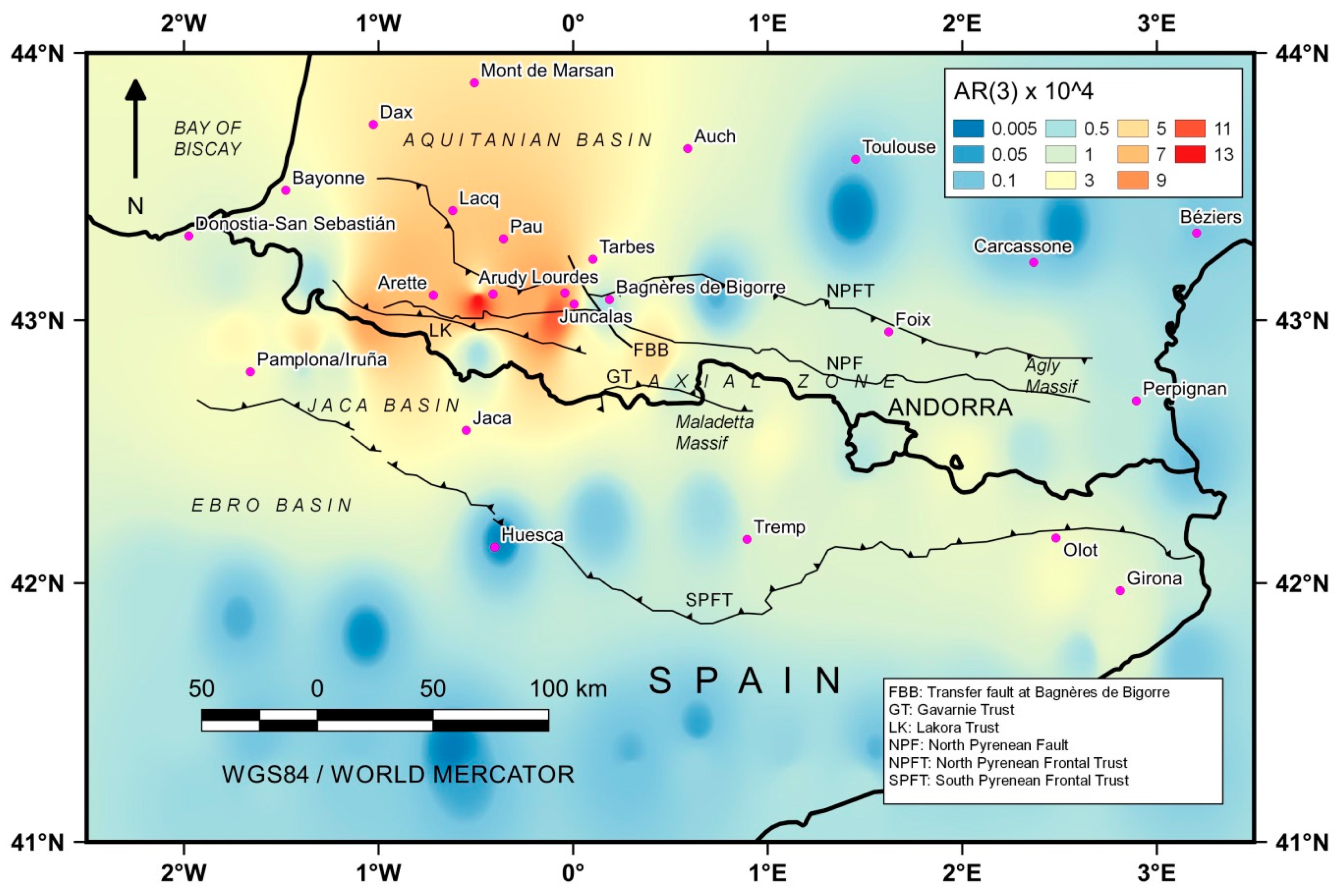
Finally, the third seismic parameter to be represented has been normalized by the surface annual rate for M3 (AR), as shown in Figure 12.
The analysis of the map indicates that the Arudy region is the most active area in the Pyrenees. In addition, it is one of the highest in the whole Iberian Peninsula and its surroundings, compared with [6,7] (for M3). An AR value exceeding 12 events every year × 10−4/km2 is higher than any other, as it is about 7–9 near Granada in the Betics. Other regions with higher values are in the central-western area (six or more) and particularly near Lourdes (greater than 10). On the contrary, in the east is unlikely to reach three. In a considerable extension of south territory, almost no zones get 1, as in the northeast.
These data are consistent with those calculated by IGN-UPM-WorkingGroup [2], where both Z16 for GM12 zonation and Z15 for A12 are among the most active zones in the Iberian Peninsula and adjacent areas.
After these results, the environment of Arudy and Bagnères de Bigorre has the most pronounced seismicity, as Mmax and AR are high, and the b-value is lower than in the rest of the Pyrenees.
5. Conclusions
This paper presents the calculation, continuous representation, and analysis of some of the most relevant seismic parameters for the Pyrenees range. These parameters are the maximum magnitude, Mmax, the b-value of the GR relation, and the annual rate AR. The information has been integrated into the GIS for calculation and visualization, which allows proper handling of the data.
For this purpose, a reliable, homogeneous, extensive, reviewed, and updated catalog has been compiled. First of all, the NGIS earthquake database (with reliable records form 1373) has been chosen as a starting point. After that, it has been reviewed with other catalog and specific studies. Then, the size of all the events has been converted to moment magnitude (Mw), as the state-of-the-art establishes, through Cabañas et al. [36]. Besides, the completeness has been analyzed, leading to set the cut-off magnitude as 2.0. Next, the non-main events have been removed by the declustering process proposed by Gardner and Knopoff [78] with the Uhrhammer [83] parameters. Later, the pairs magnitude–year of completeness have been obtained. Finally, the seismic catalog of the work is ready to be integrated into the GIS. In its environment, different grids, of 0.5 × 0.5° and 1.0 × 1.0°, have been established to produce continuous representation.
Concerning the results for the seismic parameters, some findings can be stated. The Mmax value ranges from 6.7 to no data (or M < 2) in some grids’ cells. Through the belt, near the Spain–France border, most of the zones have M5+. The maximum values are located in the Bagnères de Bigorre region, and to the north of Olot (Eastern Pyrenees), in Spain.
The b-value calculations have employed more than 200 years to include historical events. Furthermore, the method proposed by Kijko and Smit [13], which considers different pairs of magnitude–year of completeness, has been used. The lower values (so, higher stress held) have been found in the Central area, near Bagnères de Bigorre (0.97) and to the west to reach 1.05 in the Arudy region, and 1.17 in the Arette region. In both extremes of east and west, the values are approximately 1.15–1.18.
The AR for M3 shows that the Arudy region is the most active area in the belt. Besides, the Bagnères de Bigorre area shows high AR values too, with AR values higher than 10−4 earthquakes/km2 in a year.
Finally, from the analysis of the parameters, conducted by the GIS, it arises that the Central part, mainly that from Arudy to Bagnères de Bigorre, presents the most pronounced seismicity of the region, as it has the highest Mmax and AR, and the lowest b-value. Therefore, this would be the area where the PSHA should be focused on, and a GIS tool would be very handy for it.
Author Contributions
Conceptualization, José Lázaro Amaro-Mellado and Dieu Tien Bui; methodology, José Lázaro Amaro-Mellado; software, José Lázaro Amaro-Mellado; validation, José Lázaro Amaro-Mellado and Dieu Tien Bui; formal analysis, José Lázaro Amaro-Mellado and Dieu Tien Bui; investigation, José Lázaro Amaro-Mellado; resources, José Lázaro Amaro-Mellado; data curation, José Lázaro Amaro-Mellado; writing—original draft preparation, José Lázaro Amaro-Mellado; writing—review and editing, José Lázaro Amaro-Mellado and Dieu Tien Bui; visualization, José Lázaro Amaro-Mellado; supervision, José Lázaro Amaro-Mellado and Dieu Tien Bui; project administration, José Lázaro Amaro-Mellado. All authors have read and agreed to the published version of the manuscript.
Funding
This research received no external funding.
Acknowledgments
The authors would like to thank researchers from NGIS for the information, and particularly, José Manuel Martínez-Solares for his comments that have helped to enrich this document.
Conflicts of Interest
The authors declare no conflict of interest.
References
- Mezcua, J.; Rueda, J.; García Blanco, R.M. A new probabilistic seismic hazard study of Spain. Nat. Hazards 2011, 59, 1087–1108. [Google Scholar] [CrossRef]
- IGN-UPM-Working Group. Actualización de Mapas de Peligrosidad Sísmica 2012; Instituto Geográfico Nacional: Madrid, Spain, 2013; ISBN 9788441626850.
- Hamdache, M.; Peláez, J.A.; Kijko, A.; Smit, A.; Sawires, R. Seismic Hazard Parameters of Main Seismogenic Source Zone Model in the Algeria-Morocco Region. In Proceedings of the Geo-Risks in the Mediterranean and their Mitigation, Valletta, Malta, 20–21 July 2015; pp. 99–101. [Google Scholar]
- Hamdache, M.; Peláez, J.A.; Kijko, A.; Smit, A. Energetic and spatial characterization of seismicity in the Algeria–Morocco region. Nat. Hazards 2017, 86, 273–293. [Google Scholar] [CrossRef] [Green Version]
- Hong, T.-K.; Park, S.; Lee, J.; Kim, W. Spatiotemporal Seismicity Evolution and Seismic Hazard Potentials in the Western East Sea (Sea of Japan). Pure Appl. Geophys. 2020, 1–14. [Google Scholar] [CrossRef]
- Amaro-Mellado, J.L.; Morales-Esteban, A.; Asencio-Cortés, G.; Martínez-Álvarez, F. Comparing seismic parameters for different source zone models in the Iberian Peninsula. Tectonophysics 2017, 717, 449–472. [Google Scholar] [CrossRef]
- Amaro-Mellado, J.L.; Morales-Esteban, A.; Martínez-Álvarez, F. Mapping of seismic parameters of the Iberian Peninsula by means of a geographic information system. Cent. Eur. J. Oper. Res. 2018, 26, 739–758. [Google Scholar] [CrossRef]
- Hossain, B.; Hossain, S.S. Probabilistic estimation of seismic parameters for Bangladesh. Arab. J. Geosci. 2020, 13. [Google Scholar] [CrossRef]
- Popandopoulos, G.A.; Chatziioannou, E. Gutenberg-Richter Law Parameters Analysis Using the Hellenic Unified Seismic Network Data Through FastBee Technique. Earth Sci. 2014, 3, 122. [Google Scholar] [CrossRef]
- Sawires, R.; Santoyo, M.A.; Peláez, J.A.; Corona Fernández, R.D. An updated and unified earthquake catalog from 1787 to 2018 for seismic hazard assessment studies in Mexico. Sci. data 2019, 6, 241. [Google Scholar] [CrossRef] [Green Version]
- Mousavi, S.M. Mapping seismic moment and b-value within the continental-collision orogenic-belt region of the Iranian Plateau. J. Geodyn. 2017, 103, 26–41. [Google Scholar] [CrossRef]
- Beirlant, J.; Kijko, A.; Reynkens, T.; Einmahl, J.H.J. Estimating the maximum possible earthquake magnitude using extreme value methodology: The Groningen case. Nat. Hazards 2019, 98, 1091–1113. [Google Scholar] [CrossRef] [Green Version]
- Kijko, A.; Smit, A. Extension of the Aki-Utsu b-Value Estimator for Incomplete Catalogs. Bull. Seismol. Soc. Am. 2012, 102, 1283–1287. [Google Scholar] [CrossRef] [Green Version]
- Ghosh, A.; Newman, A.V.; Thomas, A.M.; Farmer, G.T. Interface locking along the subduction megathrust from b-value mapping near Nicoya Peninsula, Costa Rica. Geophys. Res. Lett. 2008, 35, 1–6. [Google Scholar] [CrossRef] [Green Version]
- Mapa_Sismotectónico_WG. Análisis Sismotectónico de la Península Ibérica, Baleares y Canarias; Instituto Geográfico Nacional: Madrid, Spain, 1992; Volume 26.
- Deligiannakis, G.; Papanikolaou, I.D.; Roberts, G. Fault specific GIS based seismic hazard maps for the Attica region, Greece. Geomorphology 2018, 306, 264–282. [Google Scholar] [CrossRef] [Green Version]
- De Donatis, M.; Pappafico, G.; Romeo, R. A Field Data Acquisition Method and Tools for Hazard Evaluation of Earthquake-Induced Landslides with Open Source Mobile GIS. ISPRS Int. J. Geo-Information 2019, 8, 91. [Google Scholar] [CrossRef] [Green Version]
- Tien Bui, D.; Shahabi, H.; Omidvar, E.; Shirzadi, A.; Geertsema, M.; Clague, J.; Khosravi, K.; Pradhan, B.; Pham, B.; Chapi, K.; et al. Shallow Landslide Prediction Using a Novel Hybrid Functional Machine Learning Algorithm. Remote Sens. 2019, 11, 931. [Google Scholar] [CrossRef] [Green Version]
- Naegeli, T.J.; Laura, J. Back-projecting secondary craters using a cone of uncertainty. Comput. Geosci. 2019, 123, 1–9. [Google Scholar] [CrossRef]
- Gutenberg, B.; Richter, C.F. Seismicity of the Earth; Princeton University: Princeton, NJ, USA, 1954. [Google Scholar]
- Udías, A.; Mezcua, J. Fundamentos de Geofísica; Alianza Universidad Textos; Alianza Editorial: Madrid, Spain, 1997. [Google Scholar]
- Hiemer, S.; Woessner, J.; Basili, R.; Danciu, L.; Giardini, D.; Wiemer, S. A smoothed stochastic earthquake rate model considering seismicity and fault moment release for Europe. Geophys. J. Int. 2014, 198, 1159–1172. [Google Scholar] [CrossRef] [Green Version]
- Frohlich, C.; Davis, S.D. Teleseismic b values; Or, much ado about 1.0. J. Geophys. Res. 1993, 98, 631–644. [Google Scholar] [CrossRef]
- Nava, F.A.; Ávila-Barrientos, L.; Márquez-Ramírez, V.H.; Torres, I.; Zúñiga, F.R. Sampling uncertainties and source b likelihood for the Gutenberg-Richter b value from the Aki-Utsu method. J. Seismol. 2018, 22, 315–324. [Google Scholar] [CrossRef]
- Tormann, T.; Wiemer, S.; Mignan, A. Systematic survey of high-resolution b value imaging along Californian faults: Inference on asperities. J. Geophys. Res. Solid Earth 2014, 119, 2029–2054. [Google Scholar] [CrossRef]
- Morales-Esteban, A.; Martínez-Álvarez, F.; Reyes, J. Earthquake prediction in seismogenic areas of the Iberian Peninsula based on computational intelligence. Tectonophysics 2013, 593, 121–134. [Google Scholar] [CrossRef]
- Rigo, A.; Souriau, A.; Sylvander, M. Spatial variations of b-value and crustal stress in the Pyrenees. J. Seismol. 2018, 22, 337–352. [Google Scholar] [CrossRef]
- Amorèse, D.; Grasso, J.R.; Rydelek, P.A. On varying b-values with depth: Results from computer-intensive tests for Southern California. Geophys. J. Int. 2010, 180, 347–360. [Google Scholar] [CrossRef] [Green Version]
- Pandey, A.K.; Chingtham, P.; Roy, P.N.S. Homogeneous earthquake catalogue for Northeast region of India using robust statistical approaches. Geomatics, Nat. Hazards Risk 2017, 1–15. [Google Scholar] [CrossRef] [Green Version]
- Haque, D.M.E.; Chowdhury, S.H.; Khan, N.W. Intensity Attenuation Model Evaluation for Bangladesh with Respect to the Surrounding Potential Seismotectonic Regimes. Pure Appl. Geophys. 2020, 177, 157–179. [Google Scholar] [CrossRef]
- Waseem, M.; Khan, S.; Asif Khan, M. Probabilistic Seismic Hazard Assessment of Pakistan Territory Using an Areal Source Model. Pure Appl. Geophys. 2020. [Google Scholar] [CrossRef]
- Peláez, J.A.; Chourak, M.; Tadili, B.A.; Aït Brahim, L.; Hamdache, M.; López Casado, C.; Martínez Solares, J.M. A catalog of main Moroccan earthquakes from 1045 to 2005. Seismol. Res. Lett. 2007, 78, 614–621. [Google Scholar] [CrossRef]
- Hamdache, M.; Pelaez, J.A.; Talbi, A.; Casado, C.L. A Unified Catalog of Main Earthquakes for Northern Algeria from A.D. 856 to 2008. Seismol. Res. Lett. 2010, 81, 732–739. [Google Scholar] [CrossRef] [Green Version]
- Zare, M.; Amini, H.; Yazdi, P.; Sesetyan, K.; Demircioglu, M.B.; Kalafat, D.; Erdik, M.; Giardini, D.; Khan, M.A.; Tsereteli, N. Recent developments of the Middle East catalog. J. Seismol. 2014, 18, 749–772. [Google Scholar] [CrossRef]
- Das, R.; Sharma, M.L.; Wason, H.R.; Choudhury, D.; Gonzalez, G. A seismic moment magnitude scale. Bull. Seismol. Soc. Am. 2019, 109, 1542–1555. [Google Scholar] [CrossRef]
- Cabañas, L.; Rivas-Medina, A.; Martínez-Solares, J.M.; Gaspar-Escribano, J.M.; Benito, B.; Antón, R.; Ruiz-Barajas, S. Relationships Between M w and Other Earthquake Size Parameters in the Spanish IGN Seismic Catalog. Pure Appl. Geophys. 2015, 172, 2397–2410. [Google Scholar] [CrossRef]
- Scordilis, E.M. Empirical Global Relations Converting MS and mb to Moment Magnitude. J. Seismol. 2006, 10, 225–236. [Google Scholar] [CrossRef]
- Njike-Kassala, J.-D.; Souriau, A.; Gagnepain-Beyneix, J.; Martel, L.; Vadell, M. Frequency-magnitude relationship and Poisson’s ratio in the Pyrenees, in relation to earthquake distribution. Tectonophysics 1992, 215, 363–369. [Google Scholar] [CrossRef]
- Rigo, A.; Pauchet, H.; Souriau, A.; Grésillaud, A.; Nicolas, M.; Olivera, C.; Figueras, S. The February 1996 earthquake sequence in the eastern Pyrenees: First results. J. Seismol. 1997, 1, 3–14. [Google Scholar] [CrossRef]
- Vissers, R.L.M.; Meijer, P.T. Iberian plate kinematics and Alpine collision in the Pyrenees. Earth-Science Rev. 2012, 114, 61–83. [Google Scholar] [CrossRef]
- Lacan, P.; Ortuño, M. Active Tectonics of the Pyrenees: A review. J. Iber. Geol. 2012, 38, 9–30. [Google Scholar] [CrossRef] [Green Version]
- Singh, C. Spatial variation of seismic b-values across the NW Himalaya. Geomat. Nat. Hazards Risk 2016, 7, 522–530. [Google Scholar] [CrossRef]
- Souriau, A.; Rigo, A.; Sylvander, M.; Benahmed, S.; Grimaud, F. Seismicity in central-western Pyrenees (France): A consequence of the subsidence of dense exhumed bodies. Tectonophysics 2014, 621, 123–131. [Google Scholar] [CrossRef]
- Teixell, A.; Labaume, P.; Lagabrielle, Y. The crustal evolution of the west-central Pyrenees revisited: Inferences from a new kinematic scenario. Comptes Rendus-Geosci. 2016, 348, 257–267. [Google Scholar] [CrossRef] [Green Version]
- Roigé, M.; Gómez-Gras, D.; Remacha, E.; Daza, R.; Boya, S. Tectonic control on sediment sources in the Jaca basin (Middle and Upper Eocene of the South-Central Pyrenees). Comptes Rendus-Geosci. 2016, 348, 236–245. [Google Scholar] [CrossRef]
- Baize, S.; Cushing, E.M.; Lemeille, F.; Jomard, H. Updated seismotectonic zoning scheme of Metropolitan France, with reference to geologic and seismotectonic data. Bull. la Soc. Geol. Fr. 2013, 184, 225–259. [Google Scholar] [CrossRef]
- Olivera, C.; Redondo, E.; Lambert, J.; Riera-Melis, A.; Roca, A. Els terratrèmols de segles XIV i XV a Catalunya; Institut Cartogràfic de Catalunya: Barcelona, Spain, 2006; ISBN 8439369611. [Google Scholar]
- Insitituto Geográfico Nacional Terremotos más Importantes. Available online: https://www.ign.es/web/ign/portal/terremotos-importantes (accessed on 29 April 2020).
- Perea, H. The Catalan seismic crisis (1427 and 1428; NE Iberian Peninsula): Geological sources and earthquake triggering. J. Geodyn. 2009, 47, 259–270. [Google Scholar] [CrossRef] [Green Version]
- Honoré, L.; Courboulex, F.; Souriau, A. Ground motion simulations of a major historical earthquake (1660) in the French Pyrenees using recent moderate size earthquakes. Geophys. J. Int. 2011, 187, 1001–1018. [Google Scholar] [CrossRef] [Green Version]
- Cara, M.; Alasset, P.J.; Sira, C. Magnitude of Historical Earthquakes, from Macroseismic Data to Seismic Waveform Modelling: Application to the Pyrenees and a 1905 Earthquake in the Alps. In Historical Seismology. Modern Approaches in Solid Earth Sciences; Fréchet, J., Meghraoui, M., Stucchi, M., Eds.; Springer: Cham, Switzerland, 2008; Volume 2, pp. 369–384. [Google Scholar]
- Rigo, A.; Massonnet, D. Investigating the 1996 Pyrenean Earthquake (France) with SAR interferograms heavily distorted by atmosphere. Geophys. Res. Lett. 1999, 26, 3217–3220. [Google Scholar] [CrossRef]
- Ministerio de Fomento (Gobierno de España). Norma de la Construcción Sismorresistente Española (NCSE-02); Boletín Oficial del Estado: Madrid, Spain, 2002.
- Gallart, J.; Dainières, M.; Banda, E.; Suriñach, E.; Hirn, A. The eastern Pyrenean domain: Lateral variations at crust-mantle level. Ann. Geophys. 1980, 36, 141–158. [Google Scholar]
- Sylvander, M.; Souriau, A.; Rigo, A.; Tocheport, A.; Toutain, J.-P.; Ponsolles, C.; Benahmed, S. The 2006 November, M L = 5.0 earthquake near Lourdes (France): New evidence for NS extension across the Pyrenees. Geophys. J. Int. 2008, 175, 649–664. [Google Scholar] [CrossRef] [Green Version]
- Secanell, R.; Martin, C.; Goula, X.; Susagna, T.; Tapia, M.; Bertil, D. Evaluacion probabilista de la peligrosidad sísmica de la región pirenaica. In 3° Congreso Nacional de Ingeniería Sísmica; Asociación Española de Ingeniería Sísmica: Madrid, Spain, 2007; pp. 1–17. [Google Scholar]
- Secanell, R.; Bertil, D.; Martin, C.; Goula, X.; Susagna, T.; Tapia, M.; Dominique, P.; Carbon, D.; Fleta, J. Probabilistic seismic hazard assessment of the Pyrenean region. J. Seismol. 2008, 12, 323–341. [Google Scholar] [CrossRef]
- Rigo, A.; Vernant, P.; Feigl, K.L.; Goula, X.; Khazaradze, G.; Talaya, J.; Morel, L.; Nicolas, J.; Baize, S.; Chery, J.; et al. Present-day deformation of the Pyrenees revealed by GPS surveying and earthquake focal mechanisms until 2011. Geophys. J. Int. 2015, 201, 947–964. [Google Scholar] [CrossRef] [Green Version]
- Insitituto Geográfico Nacional Catálogo de Terremotos. Available online: http://www.ign.es/web/ign/portal/sis-catalogo-terremotos (accessed on 29 April 2020).
- González, Á. The Spanish National Earthquake Catalogue: Evolution, precision and completeness. J. Seismol. 2017, 21, 435–471. [Google Scholar] [CrossRef]
- Mezcua, J.; Rueda, J.; Blanco, R.M.G. Reevaluation of historic Earthquakes in Spain. Seismol. Res. Lett. 2004, 75, 75–81. [Google Scholar] [CrossRef]
- Martínez-Solares, J.M.; Mezcua, J. Catálogo Sísmico de la Península Ibérica (800 a. C.-1900); Instituto Geográfico Nacional: Madrid, Spain, 2002.
- Susagna, T.; Roca, A.; Goula1, X.; Batlló, J. Analysis of macroseismic and instrumental data for the study of the 19 November 1923 earthquake in the Aran Valley (Central Pyrenees). Nat. Hazards 1994, 10, 7–17. [Google Scholar] [CrossRef]
- Martín, R.; Stich, D.; Morales, J.; Mancilla, F. Moment tensor solutions for the Iberian-Maghreb region during the IberArray deployment (2009–2013). Tectonophysics 2015, 663, 261–274. [Google Scholar] [CrossRef] [Green Version]
- García-Mayordomo, J.; Insua-Arévalo, J.M. Seismic hazard assessment for the Itoiz dam site (Western Pyrenees, Spain). Soil Dyn. Earthq. Eng. 2011, 31, 1051–1063. [Google Scholar] [CrossRef]
- Stich, D.; Ammon, C.J.; Morales, J. Moment tensor solutions for small and moderate earthquakes in the Ibero-Maghreb region. J. Geophys. Res. Solid Earth 2003, 108. [Google Scholar] [CrossRef]
- Stich, D.; Martín, R.; Batlló, J.; Macià, R.; Mancilla, F.d.L.; Morales, J. Normal Faulting in the 1923 Berdún Earthquake and Postorogenic Extension in the Pyrenees. Geophys. Res. Lett. 2018, 45, 3026–3034. [Google Scholar] [CrossRef]
- Mezcua, J.; Martínez-Solares, J.M. Sismicidad del área Íbero-Magrebí; Instituto Geográfico Nacional: Madrid, Spain, 1983; Volume 203.
- Veith, K.F.; Clawson, G.E. Magnitude from short period P-wave data. Bull. Seismol. Soc. Am. 1972, 62, 435–452. [Google Scholar]
- López, C. Nuevas fórmulas de Magnitud para la Península Ibérica y su Entorno; Universidad Complutense de: Madrid, Spain, 2008. [Google Scholar]
- Das, R.; Wason, H.R.; Gonzalez, G.; Sharma, M.L.; Choudhury, D.; Lindholm, C.; Roy, N.; Salazar, P. Earthquake magnitude conversion problem. Bull. Seismol. Soc. Am. 2018, 108, 1995–2007. [Google Scholar] [CrossRef]
- Johnston, A.C. Seismic moment assessment of earthquakes in stable continental regions-I. Instrumental seismicity. Geophys. J. Int. 1996, 124, 381–414. [Google Scholar] [CrossRef]
- Johnston, A.C. Seismic moment assessment of earthquakes in stable continental regions-II. Historical seismicity. Geophys. J. Int. 1996, 125, 639–678. [Google Scholar] [CrossRef] [Green Version]
- Castellaro, S.; Mulargia, F.; Kagan, Y.Y. Regression problems for magnitudes. Geophys. J. Int. 2006, 165, 913–930. [Google Scholar] [CrossRef]
- Mignan, A.; Woessner, J. Estimating the Magnitude of Completeness for Earthquake Catalogs. CORSSA (Community Online Resource for Statistical Seismicity Analysis). 2012, pp. 1–45. Available online: https://tcs.ah-epos.eu/eprints/1587/ (accessed on 29 April 2020).
- Page, M.T.; van der Elst, N.; Hardebeck, J.; Felzer, K.; Michael, A.J. Three Ingredients for Improved Global Aftershock Forecasts: Tectonic Region, Time-Dependent Catalog Incompleteness, and Intersequence Variability. Bull. Seismol. Soc. Am. 2016, 106, 2290–2301. [Google Scholar] [CrossRef]
- Karimzadeh, S.; Matsuoka, M.; Kuang, J.; Ge, L. Spatial prediction of aftershocks triggered by a major earthquake: A binary machine learning perspective. ISPRS Int. J. Geo-Inf. 2019, 8, 462. [Google Scholar] [CrossRef] [Green Version]
- Gardner, J.K.; Knopoff, L. Is the sequence of earthquakes in Southern California, with aftershocks removed, Poissonian? Bull. Seismol. Soc. Am. 1974, 64, 1363–1367. [Google Scholar]
- Reasenberg, P. Second-order moment of Central California Seismicity, 1960–1982. J. Geophys. Res. 1985, 90, 5479–5495. [Google Scholar] [CrossRef]
- Van Stiphout, T.; Zhuang, J.; Marsan, D. Seismicity Declustering, Community Online Resource for Statistical Seismicity Analysis; ETH—Swiss Federal Institute of Technology: Zurich, Switzerland, 2012. [Google Scholar] [CrossRef]
- Khan, M.M.; Munaga, T.; Kiran, D.N.; Kumar, G.K. Seismic hazard curves for Warangal city in Peninsular India. Asian J. Civ. Eng. 2020, 21, 543–554. [Google Scholar] [CrossRef]
- Pandey, A.K.; Chingtham, P.; Prajapati, S.K.; Roy, P.N.S.; Gupta, A.K. Recent seismicity rate forecast for North East India: An approach based on rate state friction law. J. Asian Earth Sci. 2019, 174, 167–176. [Google Scholar] [CrossRef]
- Uhrhammer, R. Characteristics of Northern and Central California Seismicity. Earthq. Notes 1986, 57, 21. [Google Scholar]
- Khan, M.M.; Kalyan Kumar, G. Statistical Completeness Analysis of Seismic Data. J. Geol. Soc. India 2018, 91, 749–753. [Google Scholar] [CrossRef]
- Papadakis, G.; Vallianatos, F.; Sammonds, P. Evidence of Nonextensive Statistical Physics behavior of the Hellenic Subduction Zone seismicity. Tectonophysics 2013, 608, 1037–1048. [Google Scholar] [CrossRef]
- Wiemer, S. A Software Package to Analyze Seismicity: ZMAP. Seismol. Res. Lett. 2001, 72, 373–382. [Google Scholar] [CrossRef]
- Mulargia, F.; Tinti, S. Seismic sample areas defined from incomplete catalogues: An application to the Italian territory. Phys. Earth Planet. Int. 1985, 40, 273–300. [Google Scholar] [CrossRef]
- Tinti, S.; Mulargia, F. Confidence intervals of b values for grouped magnitudes. Bull. Seismol. Soc. Am. 1987, 77, 2125–2134. [Google Scholar]
- Wiemer, S.; Wyss, M. Minimum magnitude of completeness in earthquake catalogs: Examples from Alaska, the Western United States, and Japan. Bull. Seismol. Soc. Am. 2000, 90, 859–869. [Google Scholar] [CrossRef]
- Wesseloo, J. Addressing misconceptions regarding seismic hazard assessment in mines: B-value, Mmax, and space-time normalization. J. South. Afr. Inst. Min. Metall. 2020, 120, 67–80. [Google Scholar] [CrossRef] [Green Version]
- Kijko, A.; Singh, M. Statistical tools for maximum possible earthquake magnitude estimation. Acta Geophys. 2011, 59, 674–700. [Google Scholar] [CrossRef] [Green Version]
- Asim, K.M.; Moustafa, S.S.; Niaz, I.A.; Elawadi, E.A.; Iqbal, T.; Martínez-Álvarez, F. Seismicity analysis and machine learning models for short-term low magnitude seismic activity predictions in Cyprus. Soil Dyn. Earthq. Eng. 2020, 130, 105932. [Google Scholar] [CrossRef]
- Tan, Y.J.; Waldhauser, F.; Tolstoy, M.; Wilcock, W.S.D. Axial Seamount: Periodic tidal loading reveals stress dependence of the earthquake size distribution (b value). Earth Planet. Sci. Lett. 2019, 512, 39–45. [Google Scholar] [CrossRef] [Green Version]
- Arvanitakis, K.; Gounaropoulos, C.; Avlonitis, M. Locating Asperities by Means of Stochastic Analysis of Seismic Catalogs. Bull. Geol. Soc. Greece 2017, 50, 1293. [Google Scholar] [CrossRef] [Green Version]
- Martínez-Álvarez, F.; Reyes, J.; Morales-Esteban, A.; Rubio-Escudero, C. Determining the best set of seismicity indicators to predict earthquakes. Two case studies: Chile and the Iberian Peninsula. Knowl.-Based Syst. 2013, 50, 198–210. [Google Scholar] [CrossRef]
- Weitcher, D.H. Estimation of the earthquake recurrence parameters for unequal observation periods for different magnitudes. Bull. Seismol. Soc. Am. 1980, 70, 1337–1346. [Google Scholar]
- Kamer, Y.; Hiemer, S. Data-driven spatial b value estimation with applications to California seismicity: To b or not to b. J. Geophys. Res. Solid Earth 2015, 120, 5191–5214. [Google Scholar] [CrossRef]
- Bender, B. Maximum likelihood estimation of b values for magnitude grouped data. Bull. Seismol. Soc. Am. 1983, 73, 831–851. [Google Scholar]
- Aki, K. Maximum likelihood estimate of b in the formula logN = a-bM and its confidence limits. Bull. Earthq. Res. Inst. 1965, 43, 237–239. [Google Scholar]
- Utsu, T. A method for determining the value of b in a formula log n = a-bM showing the magnitude-frequency relation for earthquakes. Geophys. Bull. Hokkaido Univ. 1965, 13, 99–103. [Google Scholar]
- Ogata, Y.; Yamashina, K. Unbiased estimate for b-value of magnitude frequency. J. Phys. Earth 1986, 34, 187–194. [Google Scholar] [CrossRef] [Green Version]
- Shi, Y.; Bolt, B.A. The standard error of the magnitude-frequency b value. Bull. Seismol. Soc. Am. 1982, 72, 1677–1687. [Google Scholar]
- Dominique, P.; Andre, E. Probabilistic seismic hazard map on the French national territory. In Proceedings of the 12th World Conference on Earthquake Engineering, Auckland, New Zealand, 30 January–4 February 2000; pp. 1–8. [Google Scholar]
- Skordas, E.; Kulhánek, O. Spatial and temporal variations of Fennoscandian seismicity. Geophys. J. Int. 1992, 111, 577–588. [Google Scholar] [CrossRef] [Green Version]
- Roberts, N.S.; Bell, A.F.; Main, I.G. Are volcanic seismic b-values high, and if so when? J. Volcanol. Geotherm. Res. 2015, 308, 127–141. [Google Scholar] [CrossRef] [Green Version]
- Marzocchi, W.; Spassiani, I.; Stallone, A.; Taroni, M. How to be fooled searching for significant variations of the b-value. Geophys. J. Int. 2020, 220, 1845–1856. [Google Scholar] [CrossRef]
- Wiemer, S.; Wyss, M. Mapping spatial variability of the frequency-magnitude distribution of earthquakes. Adv. Geophys. 2002, 45, 259–302. [Google Scholar] [CrossRef]
- Bardainne, T.; Dubos-Sallée, N.; Sénéchal, G.; Gaillot, P.; Perroud, H. Analysis of the induced seismicity of the Lacq gas field (Southwestern France) and model of deformation. Geophys. J. Int. 2008, 172, 1151–1162. [Google Scholar] [CrossRef] [Green Version]

Figure 2.
Seismic catalog generation workflow.

Figure 3.
The National Geographic Institute of Spain (NGIS) catalog for the working area (from 1373 to 2019).
Figure 3.
The National Geographic Institute of Spain (NGIS) catalog for the working area (from 1373 to 2019).
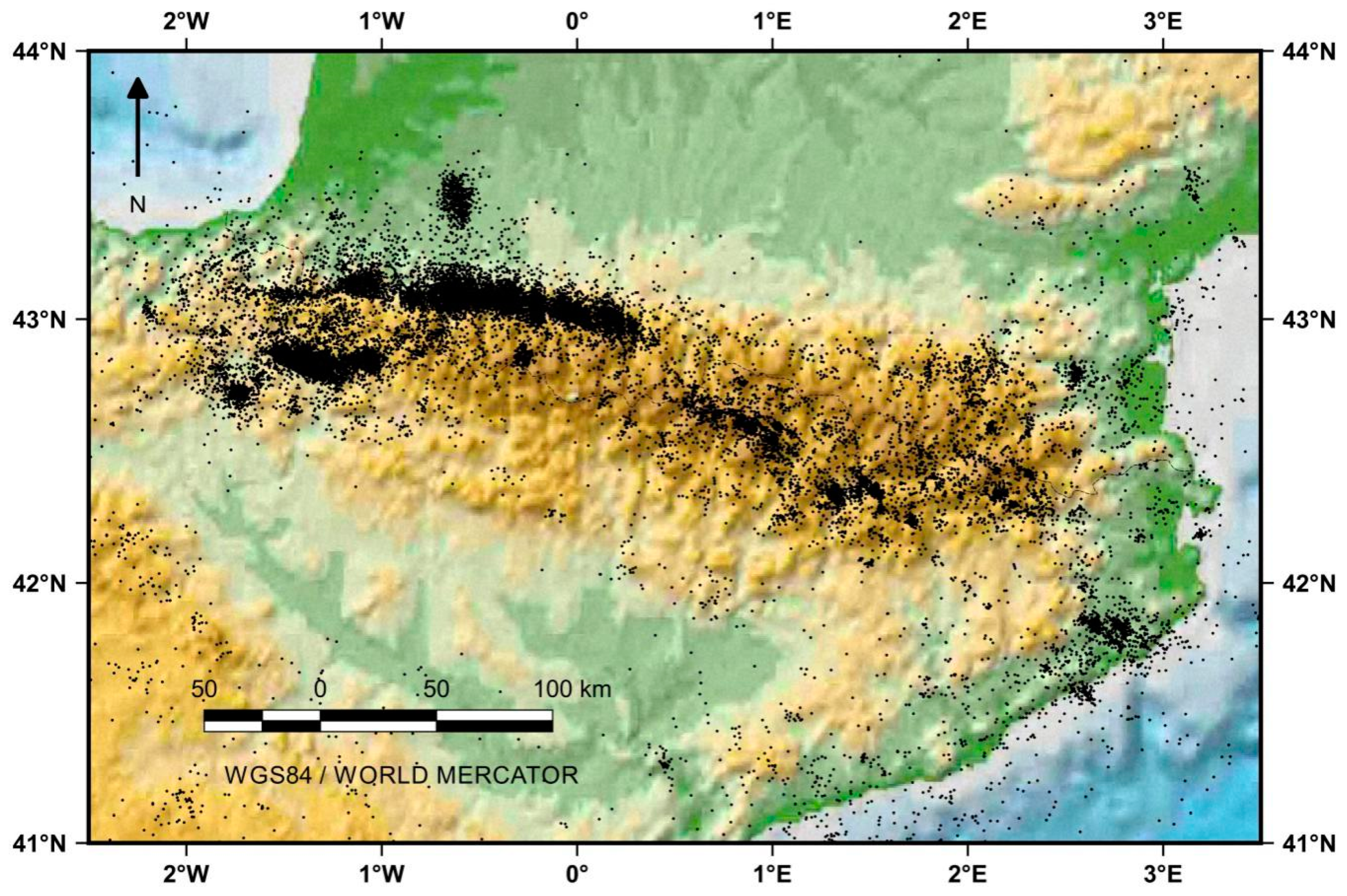
Figure 4.
The NGIS catalog (original magnitudes for the instrumental period).

Figure 5.
Frequency-magnitude (FMD) of the catalog for Mc estimation.
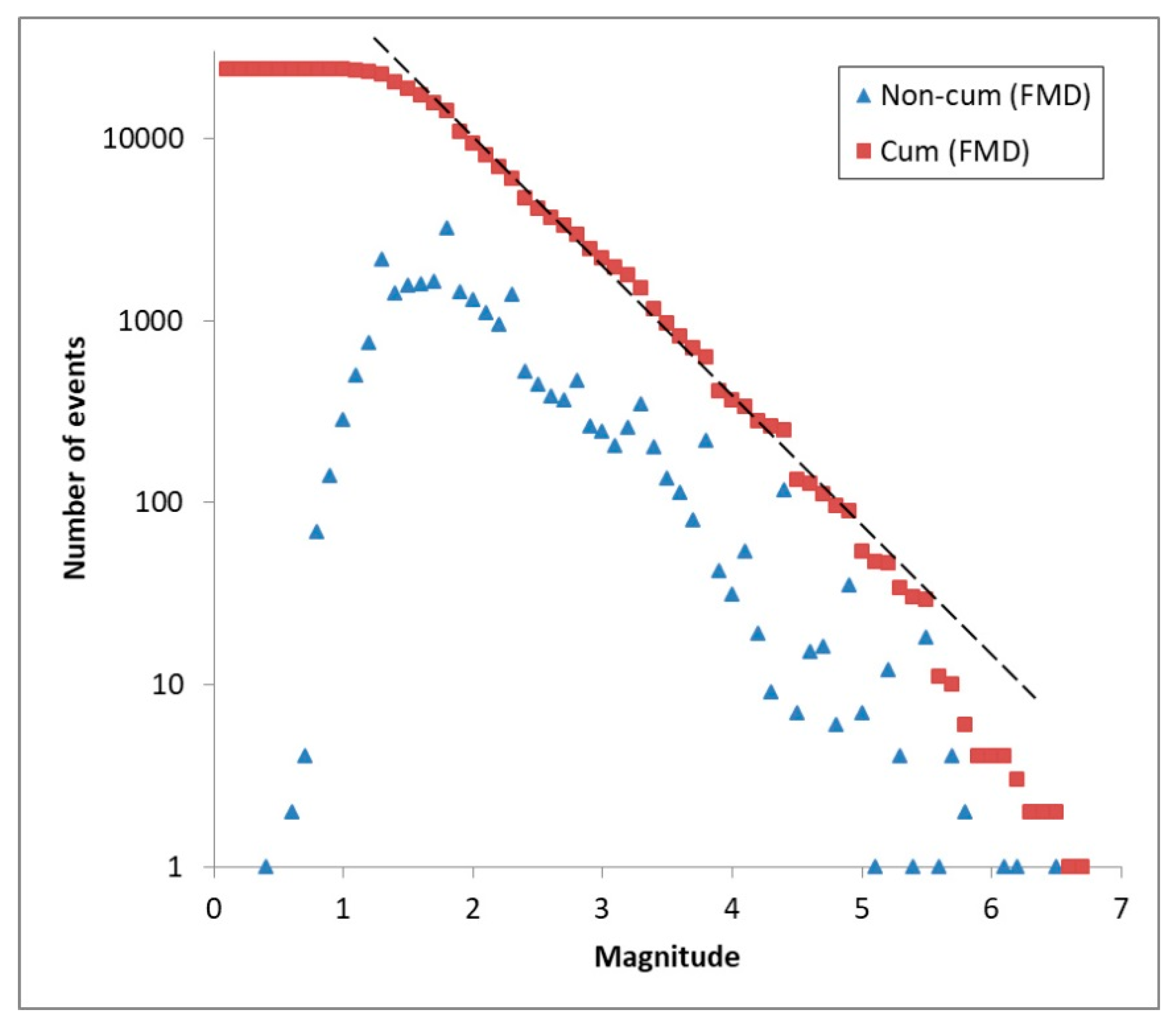
Figure 6.
Year of completeness determination from the cumulative method for different values of magnitude.
Figure 6.
Year of completeness determination from the cumulative method for different values of magnitude.
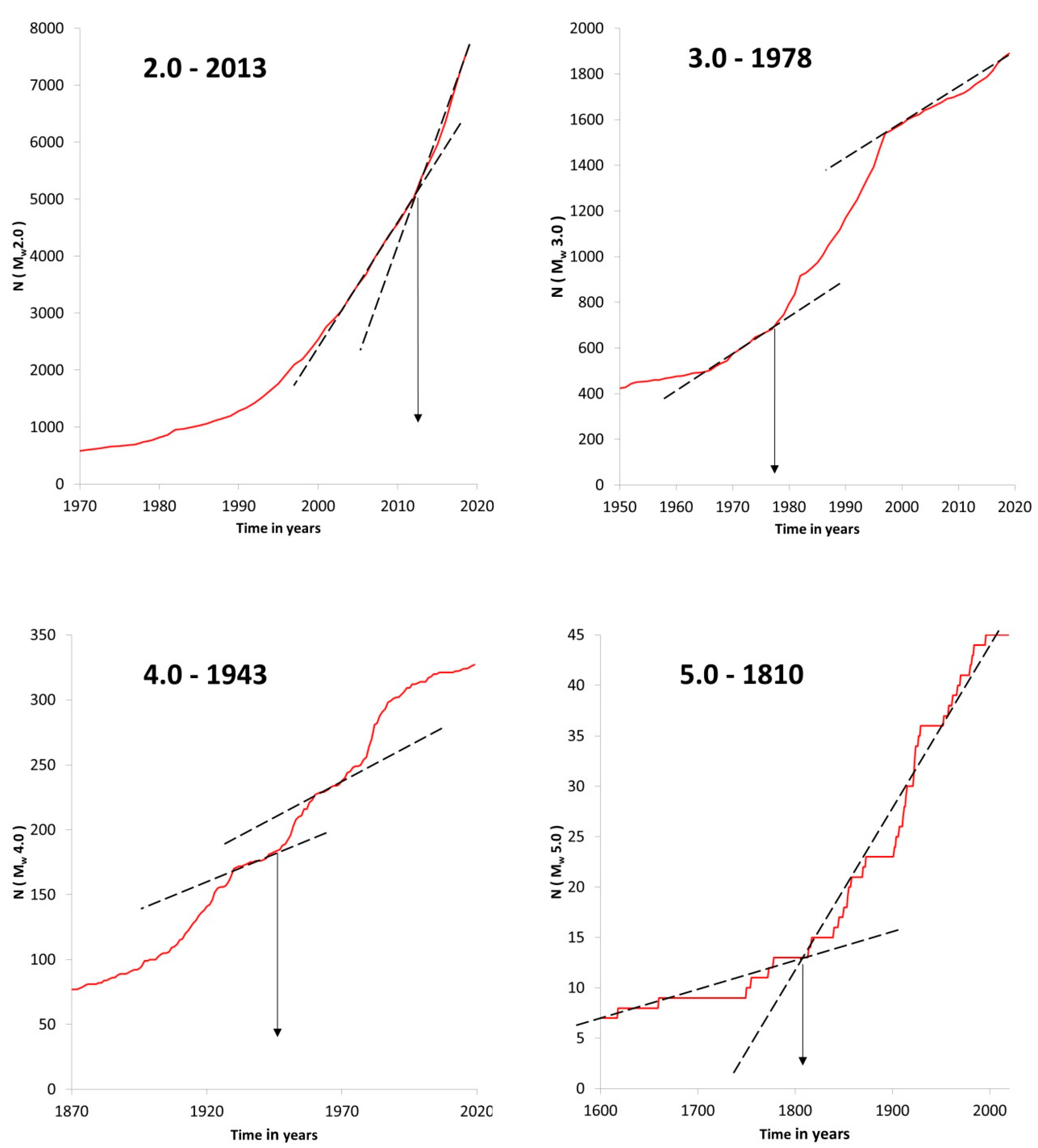
Figure 7.
Seismic catalog of the work (Mw ≥ 2.0). Temporal extent: 1373–2019.

Figure 8.
Maximum magnitude in the working catalog (1373–2019).

Figure 9.
b-value map from a 1 × 1° grid and N ≥ 50 events. A yellow point indicates that it has been used in the interpolation process.
Figure 9.
b-value map from a 1 × 1° grid and N ≥ 50 events. A yellow point indicates that it has been used in the interpolation process.
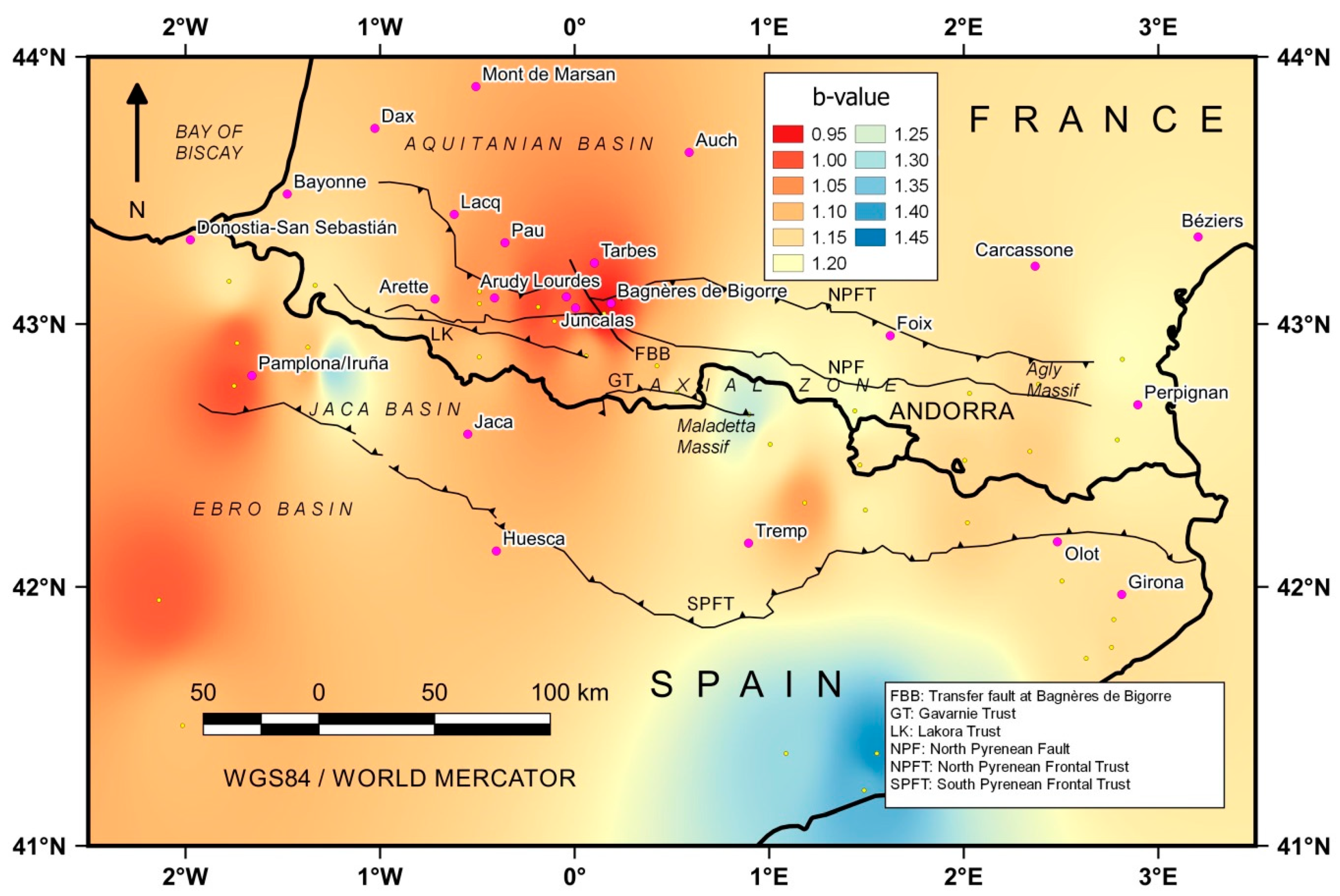
Figure 10.
Uncertainty in b-value (1 sigma) from [102]. A yellow point indicates that it has been used in the interpolation process.
Figure 10.
Uncertainty in b-value (1 sigma) from [102]. A yellow point indicates that it has been used in the interpolation process.
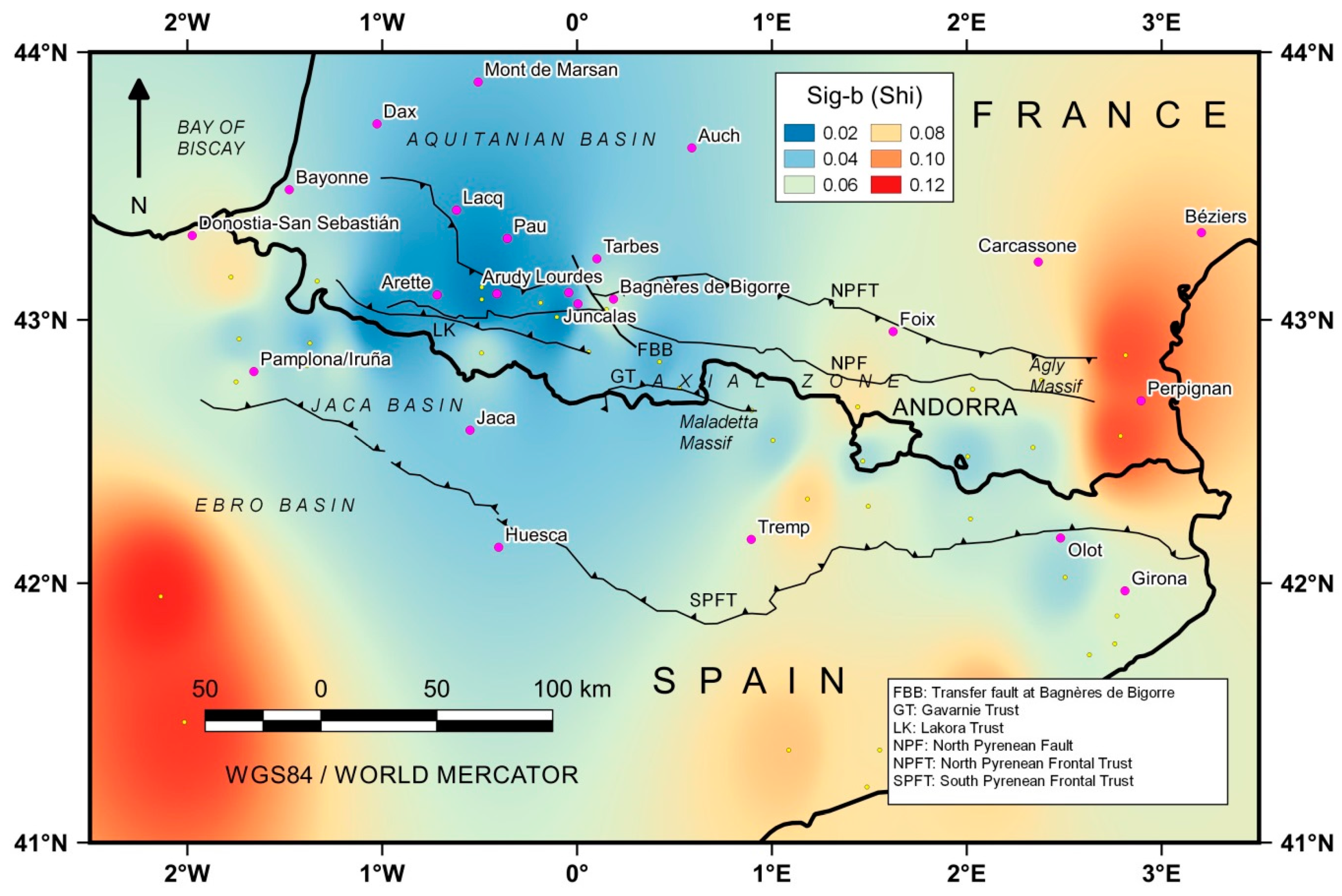
Figure 11.
b-value map from a 0.5 × 0.5° grid and N ≥ 100 events. A yellow point indicates that it has been used in the interpolation process.
Figure 11.
b-value map from a 0.5 × 0.5° grid and N ≥ 100 events. A yellow point indicates that it has been used in the interpolation process.
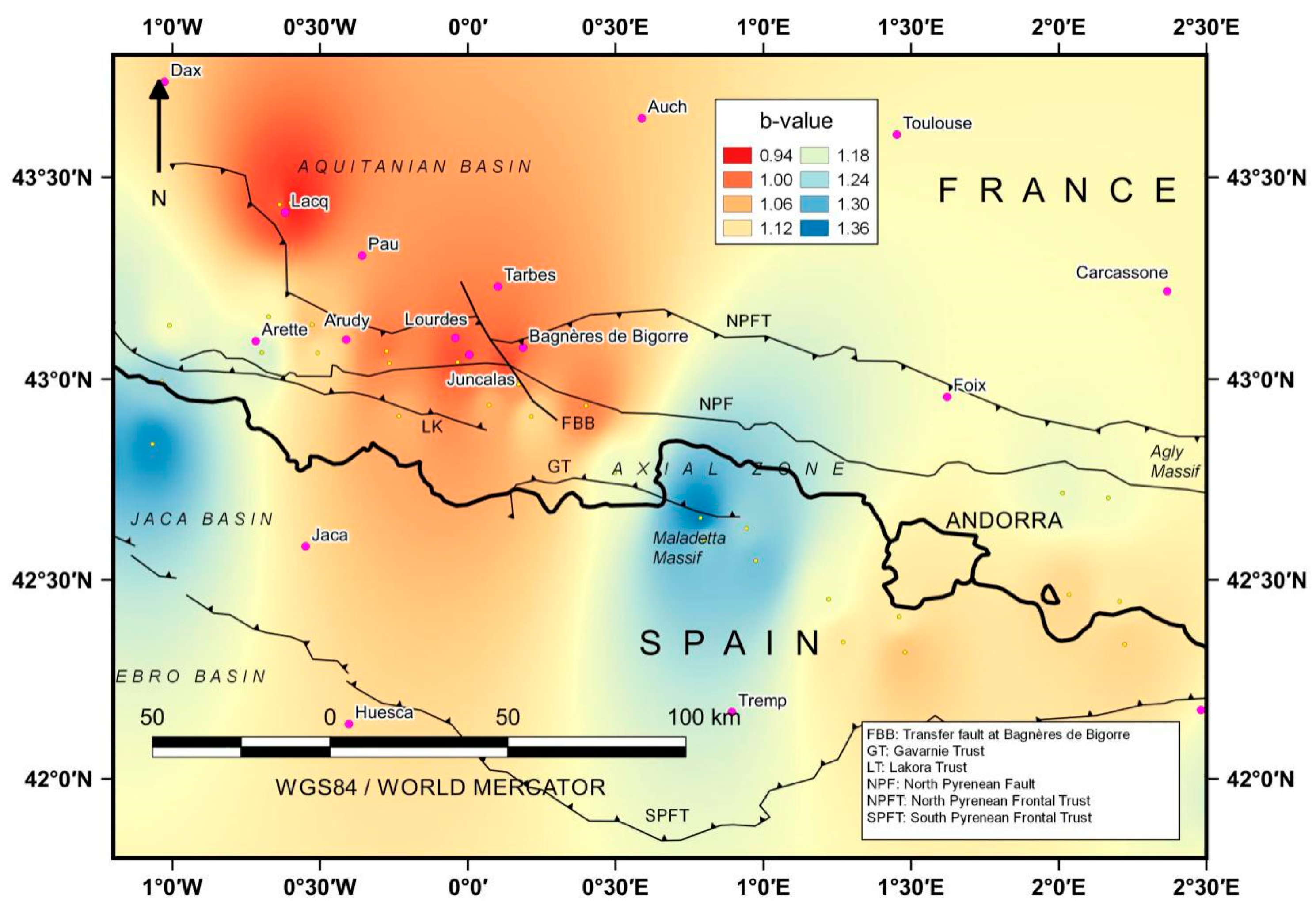
Figure 12.
Annual rate (normalized) for M3+.

Table 1.
Year of completeness vs. magnitude.
| Magnitude | Year |
|---|---|
| Mw ≥ 2.0 | 2013 |
| Mw ≥ 3.0 | 1978 |
| Mw ≥ 4.0 | 1943 |
| Mw ≥ 5.0 | 1810 |
Table 2.
Sub-catalog division (MC-Years).
| Magnitude | Year |
|---|---|
| Mw ≥ 2.0 | 2013–2019 |
| Mw ≥ 3.0 | 1978–2012 |
| Mw ≥ 4.0 | 1943–1977 |
| Mw ≥ 5.0 | 1810–1942 |
© 2020 by the authors. Licensee MDPI, Basel, Switzerland. This article is an open access article distributed under the terms and conditions of the Creative Commons Attribution (CC BY) license (http://creativecommons.org/licenses/by/4.0/).
Share and Cite
MDPI and ACS Style
Amaro-Mellado, J.L.; Tien Bui, D. GIS-Based Mapping of Seismic Parameters for the Pyrenees. ISPRS Int. J. Geo-Inf. 2020, 9, 452. https://0-doi-org.brum.beds.ac.uk/10.3390/ijgi9070452
AMA Style
Amaro-Mellado JL, Tien Bui D. GIS-Based Mapping of Seismic Parameters for the Pyrenees. ISPRS International Journal of Geo-Information. 2020; 9(7):452. https://0-doi-org.brum.beds.ac.uk/10.3390/ijgi9070452
Chicago/Turabian StyleAmaro-Mellado, José Lázaro, and Dieu Tien Bui. 2020. "GIS-Based Mapping of Seismic Parameters for the Pyrenees" ISPRS International Journal of Geo-Information 9, no. 7: 452. https://0-doi-org.brum.beds.ac.uk/10.3390/ijgi9070452
Note that from the first issue of 2016, this journal uses article numbers instead of page numbers. See further details here.