Article

A Deep Learning Approach to Urban Street Functionality Prediction Based on Centrality Measures and Stacked Denoising Autoencoder

1
Department of Geomatics, Civil Engineering, Shahid Rajaee Teacher Training University, Lavizan 1678815811, Iran
2
Department of Computing Sciences, Texas A&M university- Corpus Christi, Corpus Christi, TX 78412, USA
3
Computer Science Department, Southern Connecticut State University, New Haven, CT 06515, USA
4
Department of Civil, Geological, and Mining Engineering, Polytechnique Montréal, QC H3T 1J4, Canada
*
Author to whom correspondence should be addressed.
These authors contributed equally to this work.
ISPRS Int. J. Geo-Inf. 2020, 9(7), 456; https://0-doi-org.brum.beds.ac.uk/10.3390/ijgi9070456
Submission received: 6 June 2020 / Revised: 13 July 2020 / Accepted: 15 July 2020 / Published: 20 July 2020

Abstract

:
In urban planning and transportation management, the centrality characteristics of urban streets are vital measures to consider. Centrality can help in understanding the structural properties of dense traffic networks that affect both human life and activity in cities. Many cities classify urban streets to provide stakeholders with a group of street guidelines for possible new rehabilitation such as sidewalks, curbs, and setbacks. Transportation research always considers street networks as a connection between different urban areas. The street functionality classification defines the role of each element of the urban street network (USN). Some potential factors such as land use mix, accessible service, design goal, and administrators’ policies can affect the movement pattern of urban travelers. In this study, nine centrality measures are used to classify the urban roads in four cities evaluating the structural importance of street segments. In our work, a Stacked Denoising Autoencoder (SDAE) predicts a street’s functionality, then logistic regression is used as a classifier. Our proposed classifier can differentiate between four different classes adopted from the U.S. Department of Transportation (USDT): principal arterial road, minor arterial road, collector road, and local road. The SDAE-based model showed that regular grid configurations with repeated patterns are more influential in forming the functionality of road networks compared to those with less regularity in their spatial structure.

1. Introduction

Urban commutes using automobiles are important daily tasks for most city dwellers. The urban streets system is a vital network that connects places and people within and across urban areas. The urban street system can be effectively modeled as a network using graph theory, and the commutes become network-constrained movements [1] with each section of the network responsible to move traffic towards the destination. Having information about the elements of the network with particular objectives is very important for planners and engineers. These objectives range from long-distance traveling to serving neighborhood travel to nearby shopping centers. The functional classification of roadways defines the role each element of the roadway network plays to accommodate user needs. The spatial configuration of the street network creates constraints on movement patterns through the network. The effect of the spatial configuration of the street network on traffic flow has been studied by several researchers [2,3,4,5,6,7]. However, in our work, the spatial configuration of the network is used to classify the functionality of individual streets.
The functional classification of streets defines the role each element of the urban street network (USN) plays in the urban transportation network. Streets are usually assigned to a functional class according to their characteristics and the type of service [8] they provide. Streets help a user to access and egress from their current location toward their destination. Based on the street functionality concepts provided by the U.S. Department of Transportation (USDoT), those streets that provide a high level of mobility are called “Arterial”, those that provide a high level of accessibility are called “Local”, and those that are a balanced in term of mobility and accessibility are called “Collector”. Based on the aforementioned concepts related to street functional classification, the USNs are classified into two main groups of Arterial and Non-Arterial with Principal and Minor as sub-classes of the Arterial group, and Collector and Local street as a subclass of the Non-Arterial group. Figure 1 shows examples of several street networks categorized by functionality.
Street Functional Classification (SFC) has received additional significance beyond its purpose as a tool for identifying the particular role of streets in moving vehicles through USN. SFC has been used to describe roadway system performance, benchmarks, and targets by several transportation agencies. Aiming towards having a more performance-based approach for transportation agencies, SFC will be an increasingly important consideration in measuring outcomes mainly for preservation, mobility, and safety. So far, SFC has been achieved according to street rules and classified based on attributes such as mobility, access, trip length, speed limit, volume, annual average daily traffic (AADT), vehicle miles of travel (VMT), etc. However, evidence reveals that classification only based on the discussed elements is not enough, and streets cannot properly be classified. In many cases, assigning a functional class to a street is straightforward. However, deciding between adjacent classification is very challenging. For instance, deciding whether a given street acts as Minor Arterial or Collector can be subject to debate, because a street can be a Minor Arterial according to AADT and a collector based on VMT. Deciding between a Principal Arterial and Minor Arterial assignment can be even more challenging.
We suggest a new strategy for assigning SFC based on the spatial structure of streets and their roles in the network. Our research shows that the role of streets is more than moving the traffic. Streets are the basic skeleton of the transportation network, so describing the role of each street in the network is a significant concept. The spatial structure of streets in the network is a fundamental attribute of the network, but it has not received enough attention. The configuration of USN using semantic attributes has been analyzed [3,4,5], with recent work analyzing USN using topological [2] and geometrical attributes [9]. The Functional Classification System (FCS) was developed in the 1970s as a basis for communication between designers and planners [10,11]. It is a common framework for classifying roadways based on mobility and access [12,13,14,15]. The application of the FCS has expanded, and it is now used throughout the entire project development process and influences all transportation project development phases, from programming and planning through design and into maintenance and operation decisions [16,17,18,19].
Centrality [2] is one of the most important concepts in social network analysis; it describes spatial structural properties of nodes (streets) in a network. Several measures have been developed such as betweenness, closeness, degree centrality, eigenvector centrality, information centrality, flow betweenness, and the rush index [2]. Centrality measures have been considered individually [7,20], primarily on how they affect traffic flow. Simple statistical regression and traditional machine learning models have been used for SFC, but only based on one or two centrality measures [7]. Due to the complexity of the spatial structure of USN more parameters and measurements are needed to adequately model SFC. To consider centrality measures in urban networks, patterns of streets and roads are considered based on graph theory, which helps to extract spatial topology attributes of streets. The goal of centrality measurement is finding the most important central places in the network and their attributes that play a pivotal role in monitoring the efficiency and accessibility of transportation networks [21,22,23,24]. The centralities can help analyzers understand complex networks more effectively. Technically, centrality measurements inspired our work, where they are used to help domain users explore urban transportation data and provide initial important features from road networks to do a higher-level of analysis in the urban transportation network [25,26].
Some experimental studies demonstrate the relationship between the spatial configuration of city structure and traffic in city streets [6,9,23,27,28,29]. Along with other studies, a great deal of research has tried to unveil the movement patterns of individuals by examining the structural features of street networks. Many parameters including the network’s geometrical features, driver movement behavior, and the spatial distribution of urban land uses are influential in traffic distribution. Furthermore, research has shown that these parameters are influenced by the network’s spatial structure. For instance, the spatial structure of the urban network has a high influence on human behavior and the demand for making intra-city trips [6,30,31]. The first time a Self-Organizing Map (SOM) neural network was used in city network generalization was by Kohonen [32]. Kohonen, in his network, considered the topological, geometrical, and semantic features of the streets. Jiang and Harrie [1] utilized the SOM neural network for clustering the streets based on their features. In 2012, Zhou [33] applied SOM and Back-Propagation Neural Network (BPNN) for urban network generalization based on the city plan before city design. Their results showed improvement compared to those achieved with SOM alone.
Deep multilayer neural networks have many nonlinear levels of learning allowing them to compactly learn highly nonlinear and highly-varying functions, and have found a lot of attraction in various earth science research areas [34,35,36,37,38], particularly in urban planning problem analysis [17,39,40]. Lv et al. [40] started applying deep neural networks known as a Stacked Autoencoder (SAE) for traffic flow prediction on a big dataset. In their implementation, they achieved over 93% for traffic flow prediction. They compared their model with some traditional techniques such as Support Vector Machine (SVM), Random Forest (RF), and Back-Propagation Neural Network (BPNN), and SAE [41] achieved better results. In another research, inclement weather condition information in connection to cars is added to input features for a deep learning model for traffic flow prediction [42]. They were looking for a correlation between weather conditions and traffic flow prediction. The ability of deep learning to process big data [34,43,44], considering more correlation between datasets and solving the complexity and nonlinearity of datasets, inspired us to rethink analyzing the functionality of streets. In our work, due to having a tabular structure in the input data, a greedy layer-wise deep learning model is applied for unsupervised feature learning to understand the nonlinearity of input data and then logistic regression is used as a classifier. The SDAE model, as one of the best greedy layer-wise unsupervised models, was used to solve the problem of training deep networks [45]. For evaluating model performance, we compare several machine learning models such as logistic regression, Multi-Layer Perceptron (MLP) [46], SVM [47], and RF [48], with SDAE on four cities with different spatial structures. The four cities used are Tehran, Iran; Isfahan, Iran; Enschede, Netherlands; and Paris, France, and Figure 1 shows their spatial structure.
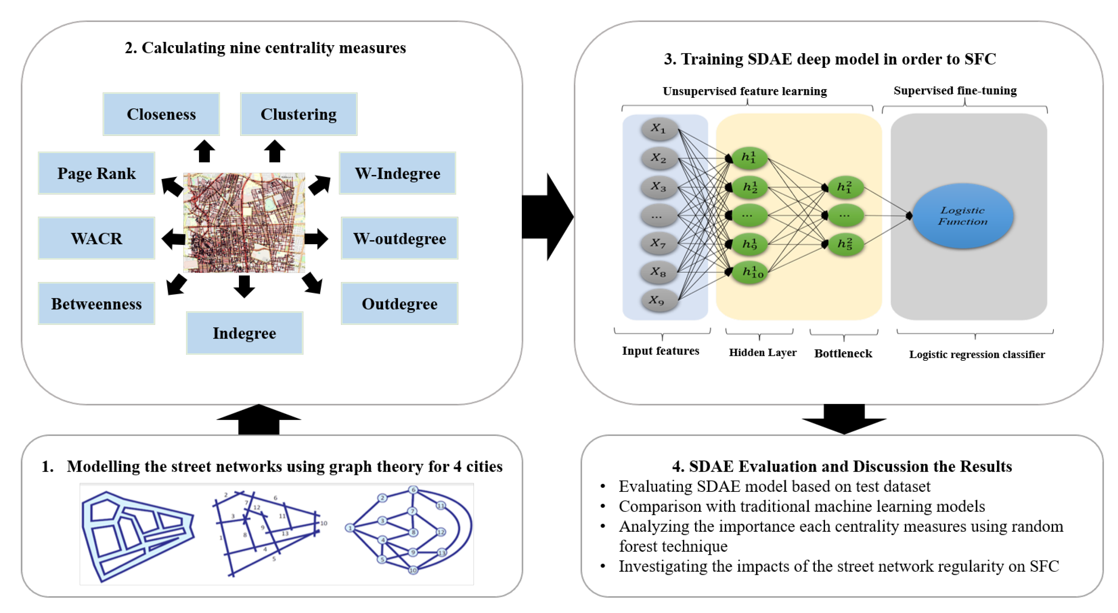
Our study proposes a method that can investigate the basic concept of a network’s manner, that is, the spatial structure of a street network. First, we prove that we can extract the functionality of a street with the spatial measurement within an acceptable percentage, and then we suggest the proposed classification method for classifying streets that do not belong to a specific functional class. In this work, first, the USN is modeled as a network using graph theory [1], then the spatial structure of the USN is described using nine centrality measurements to better understand the complexity of the network to SFC. To utilize SFC, the powerful nonlinear learning model called deep learning has been applied to take advantage of its ability to understand the complexity of the USN and street functionality. Our study investigates the structural properties of each functionality class in the real world. The major contributions of this paper are summarized as follows.
  • Considering the challenge of street functional classification based on the spatial structure of streets, mainly centrality measures.
  • Developing an unsupervised deep learning model to improve the accuracy of the street functional classification compared to traditional techniques.
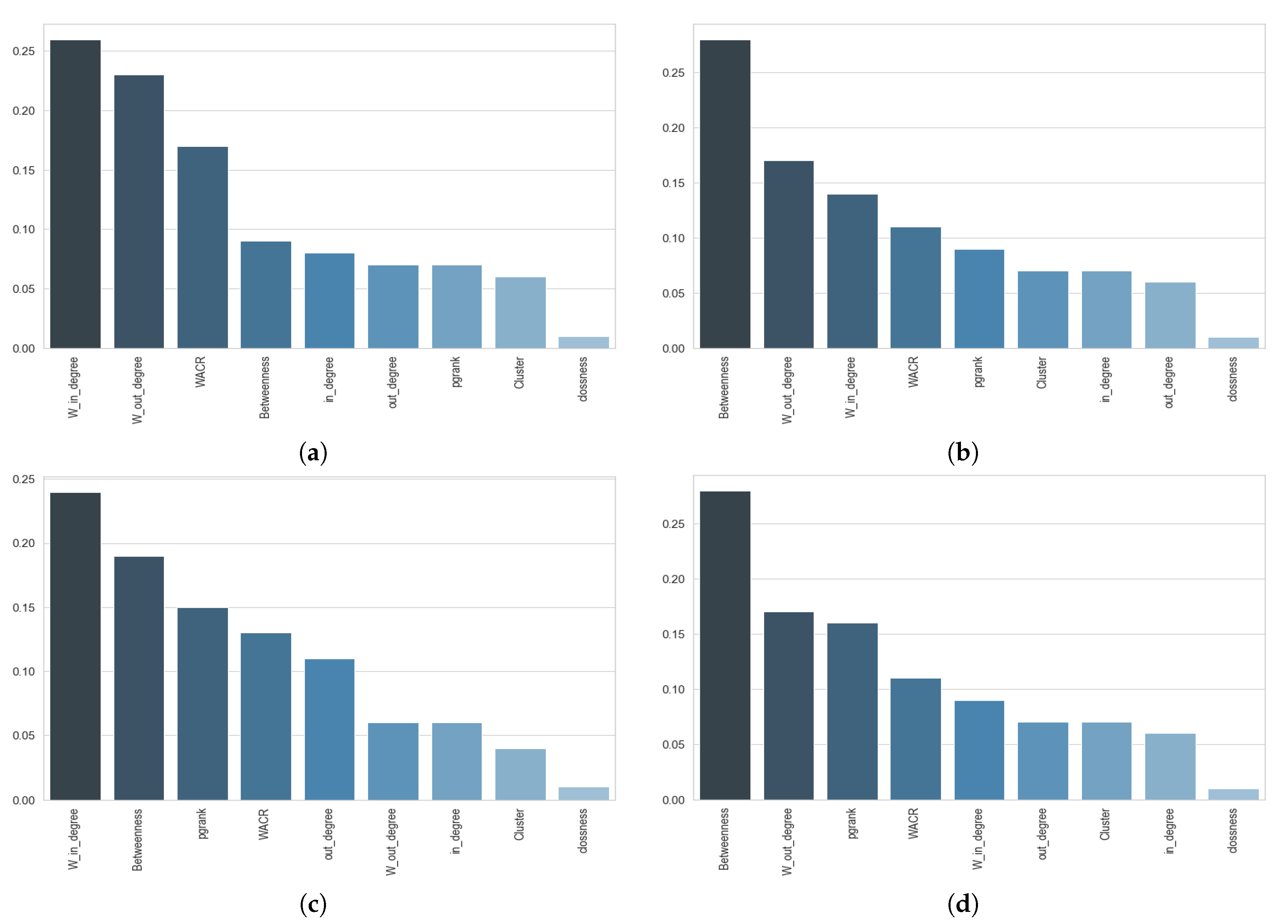
  • Analyzing the importance of each centrality measure into street functional classification by using random forest technique.
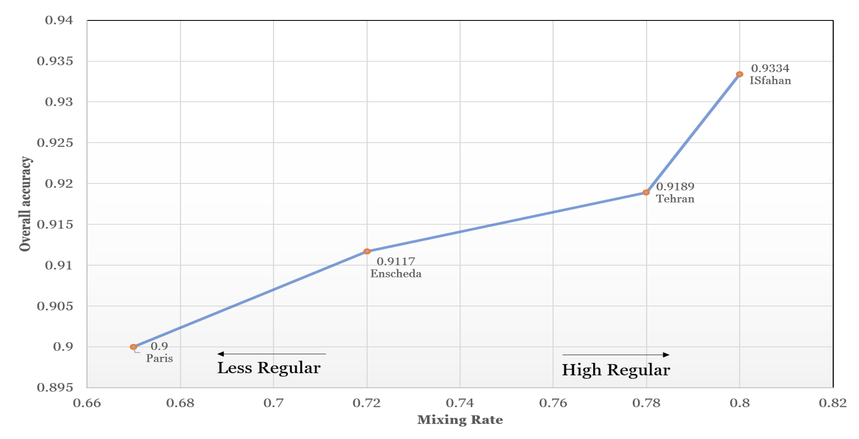
  • Investigating the impacts of the street network regularity on street functional classification.
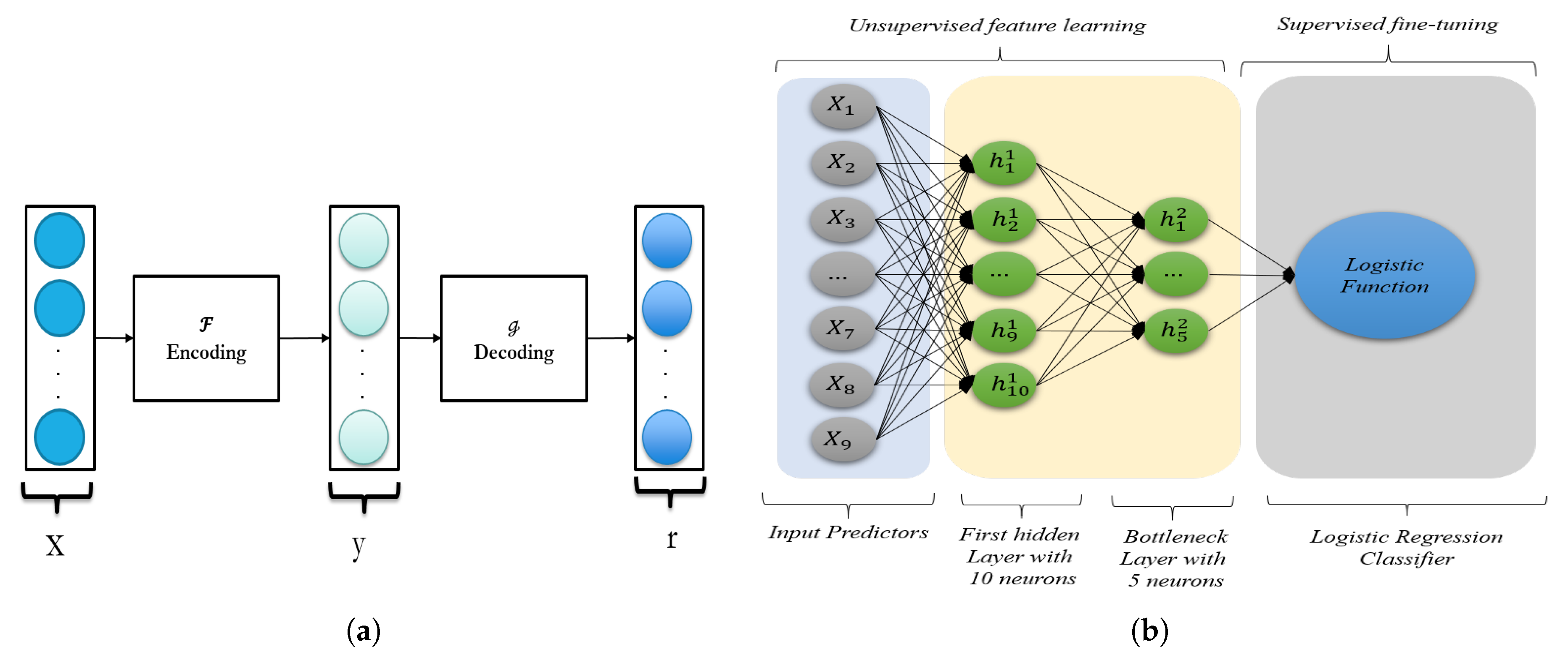
In this study, we choose a Stacked Denoising Autoencoder (SDAE) [41], as it is one of the best greedy layer-wise, unsupervised learning models [45,49]. Although our input data is labeled, we use the SDAE to learn features and weights in an unsupervised, greedy, layer-wise manner, while the supervised fine-tuning is used to further adjust the network’s weights for classification using the labeled data. For fine-tuning classification, we applied logistic regression, but other techniques would work. We compare our deep learning model with four traditional machine learning models.
The rest of the paper describes our work in detail, with Section 2 explaining SDAE and describing the centrality measures we used. Section 3 presents the methodology of our evaluation of our implementation using four different data sets. Numerical results from our experiments are discussed in Section 4, and Section 5 presents our conclusions.

2. Materials and Methods

This section explains street network modeling based on graph theory, and extracting the centrality measures used in this research for training the model. Additionally, our SDAE deep learning model is discussed. Figure 2 is a schematic of the whole process of SFC based on centrality measures using a deep learning model. At the first stage, the USN for 4 different cities studied in this work is modeled using graph theory. Then, 9 centrality measures for all cities are calculated, and their functional classes are extracted from the database. The SDAE deep learning model is then applied to SFC. Furthermore, the results are compared to traditional machine learning models. Finally, the importance of each centrality measure is considered based on the random forest technique, also the impacts of street network regularity on SFC based on mixing ratio are discussed.

2.1. USN Modeling Using Graph Theory

To model the urban street network, first, the exact concept of each street type should be defined, and second, the mathematical model for network representation should be considered. There are three methods for defining the basic element in a street network: axial line [50], segment streets, and stroke [51]. Axial lines were used in space syntax theory for modeling streets. An axial line represents the longest channels people move through in a city. Another concept used to define a street is segment streets, the connection between two intersections in the street network. Stroke is another way to define the concept of streets. The original idea of building a road segment into a stroke was proposed by Thomson and Richardson [51]. The basic principle was very simple: “Elements that appear to follow in the same direction tend to be grouped”, which follows the “principle of good continuation” theme in a visual perspective [33]. In this process, a simple geometric criterion, the deflection angle which is the deviation from 180 degrees of the angle between two road segments, was employed as a criterion for judging which two road segments should be concatenated. It was suggested to make use of a small deflection angle between 40 and 60 degrees [52] as a threshold to ensure that all the strokes follow the principle of good continuity. Moreover, in comparison with other existing methods to model the street entity, stroke usually provides better results in predicting movement patterns of individuals in urban networks [33] and is suited for traffic management and scheduling in urban networks [1].
The process of building strokes starts from an arbitrary road segment. When reaching an intersection with at least two other road segments, it is necessary to decide which one to connect to with three potential strategies: self-fit, self-best-fit, and every-best-fit [1]. The every-best-fit strategy considers every pair of road segments for comparison and selects the pair with the smallest deflection angle for concatenation. Optimum results will be obtained by using every-best-fit, as this strategy considers all possible concatenations at each intersection (for more information refer the work in [33]). The street network can be represented by a connectivity graph, consisting of vertices and edges. There is a representation of the street network based first on a primal graph, where intersections are turned into nodes and streets into edges. In a second step, a dual graph is used, where streets are nodes and intersections are edges. In our study, we use the every-best-fit method to construct strokes and also dual graphs to present street entities considering the direction of the streets. Moreover, the streets are given some weights which are determined in proportion to their lengths in the real world. Results of using this method are shown in Figure 1.

2.2. Centrality Measures

In order to analyze the spatial structure of a network, there is a need for some measures to quantify the structural features of each street in those networks. The quantification measures used to evaluate the structural features of networks are known as “centrality measures”. In this study, a total of nine measures are used to evaluate the structural importance of each street. In order to assess the structural importance of a street, it is necessary to make use of more than a single measure. As a single measure considers the importance of the street from a single point of view, utilizing a variety of evaluation measures can help us look at the problem space from different aspects. The measures used in this study are discussed below.

2.2.1. Betweenness Centrality

Betweenness centrality ( C B ) measures how often a node is traversed by the shortest path connecting all pairs of nodes in the network. C B , for node i, is defined by Equation (1):
C i B = 1 ( N 1 ) ( N 2 ) j = 1 ; k = 1 ; j k n j k ( i ) n j k
where n j k is the number of the shortest path between nodes j and k, N is total number of nodes, and n j k ( i ) is the number of the shortest paths which contain node i. Generally, nodes with higher betweenness are more involved in directing and transferring flow in the network, so they play a significant role in node communications [53]. In this study, betweenness centrality is used to identify those streets which have a bridging role between different topological shortest paths. According to the definition, this measure seems to be good for detection of high-traffic or Arterial streets. Figure 3 depicts all centrality measures include betweenness(Figure 3a) centrality for the Tehran, Iran USN.

2.2.2. In/Out-Degree and Weighted In/Out-Degree

Based on the definition by Freeman [54], the degree of a focal node i ( d e g i ) is the adjacency in the network, which means the number of directly connected nodes to the focal node i:
d e g i i n = j = 1 N a i j
d e g i o u t = j = 1 N a i j
where i is the focal node, j is all other nodes, N is the total number of nodes, and a is the adjacency matrix. To use this measure in a directed and weighted network, it is necessary to consider the direction and the weights of the connection. Regarding the direction of the connection, this measure is divided into two measures: indegree, d e g i i n , and outdegree, d e g i o u t . Indegree is the number of connections leading to a given node, and the outdegree represents the number of connections that can be accessed from that node. The degree has generally been extended to the sum of weights when analyzing weighted networks [55]. Regarding the weights of the network, this measure is divided into two measures: Weighted indegree, w d e g i i n , and Weighted outdegree, w d e g i o u t (i.e., the sum of connection weights leading to a given node or can be accessed from that node),
w d e g i i n = j = 1 N w i j
w d e g i o u t = j = 1 N w i j
where w is the weighted adjacency matrix if the node i is connected to node j, and when w i j is greater than 0, there is connection between nodes i and j. In the urban street network, the degree of each street indicates the number of streets that directly access that street which can measure the accessibility of the streets in the urban network. To use this measure in the weighted and directed street network, the direction and weight of streets (length) should also be taken into account. Figure 3b–e shows the indegree, outdegree, weighted outdegree and weighted in-degree centrality measures for Tehran.

2.2.3. Clustering Coefficient

Local clustering coefficient C L c c refers to the probability of having two adjacent nodes that are connected. This is calculated as the number of present connections over the number of possible connections between the node’s neighbors. Therefore, the outcome ranges between 0 and 1: 0 if no connections exist between the neighbors and 1 if all possible connections exist [6],
C i L c c = N a i j N p i j
where N a i j is the number of actual connections and N p i j is the number of possible connections between nodes i and j. The existence of a connection between adjacent nodes means they can send and receive network flow directly without any need for intermediation. A street with a high clustering coefficient means that its neighboring streets have direct access to each other. As a result, there is no need to cross that street to reach others, so the traffic decreases. Conversely, if there is no direct connection between the neighbors of a street, that street has a more substantial role in passing people to their destination. Figure 3f shows the clustering coefficient centrality measures for Tehran.

2.2.4. Weighted Average Centrality Rank (WACR)

This measure is developed to evaluate the amount of control each node has on the network flow. A higher value of this measure shows a more important status of the node inflow transmission in the entire network [20].
W A C R i = k i s = 1 m ( w i s + w i q w q s ) 2 ( s N i , q N i and q s )
where w i s is the ratio of the degree at node s to the sum of degree at all i’s adjacent nodes, and m is the size of the set N i . Figure 3i shows the WACR centrality measures for Tehran.

2.2.5. Page-Rank Centrality

PageRank is a key technology behind the Google search engine that decides the relevance and importance of individual web pages. Its computation is done through a web graph in which nodes and links represent individual web pages and hotlinks [56]. The web graph is a directed graph, i.e., a hotlink from page A to B does not imply another hotlink from B to A. The basic idea of PageRank is that a highly ranked node is one that highly ranked nodes point to [56], a recursive definition. PageRank is used to rank individual web pages in a hyperlinked database. It is defined formally as follows [6],
P R i L c c = 1 d n + d j O N ( i ) P R ( j ) n j
where n is the total number of nodes; O N ( i ) is the outline neighbors (i.e., those nodes that point to node i ); P R ( i ) and P R ( j ) are rank scores of nodes i and j, respectively; n j denotes the number of outline nodes of node j; and d is a damping factor, which is usually set to 0 . 85 for ranking web pages. In the urban streets network, this measure means that if a person randomly chooses routes in the urban network, the streets with high page-rank are more likely to be those passing routes. Figure 3h shows the page-rank centrality measures for Tehran.

2.2.6. Closeness Centrality

Closeness is defined as the inverse of fairness, which in turn, is the sum of distances to all other nodes [54]. The intent behind this measure was to identify the nodes which could reach others quickly. This measures to what extent node i is near to all the other nodes along the shortest paths and is defined by Equation (9):
C i C = N 1 j G ; j i d i j
where d i j is the shortest path length between i and j, defined, in a valued graph, as the smallest sum of the edge length throughout all possible paths in the graph between i and j. Figure 3g shows the closeness centrality measures for Tehran.

2.3. Regularity Measurement: Spatial Configuration of an Urban Street Network

The spatial configuration of an urban network is quite varied in different cities because they are constructed at different times and in different contexts. Social, cultural, and political factors affect the configuration and arrangement of the streets in different cities. In some cities, the configuration of roads is well disciplined and follows a uniform pattern, while in some others it is chaotic and no specific pattern can be found in them. To asses different configurations, we need a quantification measure, because two visually different configurations may be similar from the structural regularity point of view. Mixing rate is an algorithm to determine the level of structural regularity in a network.
To explain the mixing rate, consider a person who walks randomly in a network, during this random walk, they may visit some new nodes or pass nodes seen before. After taking several steps, the frequency of crossing a given node decreases until it converges to a constant value. The frequency of crossing a node is calculated as the number of times a walker passes a node divided by the total number of moves. It is proved that this frequency is in proportion to the node’s degree and is calculated as in Equation (10) [57]:
π i = d e g ( i ) E
where d e g ( i ) is the node’s degree and E is the total number of links. The rate of reduction that occurs in the frequency of crossing for network nodes is a measure used to evaluate the structural regularity level of a network [58]. This measure is defined as Equation (11):
η = lim t sup max i , j | p i j ( t ) π i | 1 t
where η is the minimum of upper boundaries or supremum. According to the definition, the supremum of the set S, which is a subset of A, if it exists, is the smallest quantity that is greater than or equal to each member of set S. The mixing rate is a measure between 0 and 1 which is determined based on the level of regularity in spatial structures.

2.4. Stacked Denoising Autoencoder

Autoencoders are a specific type of feedforward neural network with symmetric structure, which consists of one input layer, one hidden layer, and one output layer [59,60]. The middle layer, called the bottleneck, is trained to reconstruct the inputs as closely as possible. The rule of the bottleneck is compressing the input data into a lower-dimension code to force the autoencoder to learn the most informative features (latent features). The autoencoder has three functional sections: encoding to encode the input predictors and learn latent features, decoding to reconstruct the representation by using the latest features, and a loss function to calculate the errors of reconstruction [59,60]. Figure 4 gives an illustration of an autoencoder.
In the autoencoder, both the encoder and the decoder are fully-connected feedforward neural networks, and the size of the input features and the reconstructed features should be the same. However, the bottleneck layer is the heart of an autoencoder and changing it allows one to manipulate the architecture and enhance performance [59,61]. Generally, the number of nodes per layer is the most important hyperparameter for autoencoders, mostly for the bottleneck layer. The smaller the size is compared to the number of input predictors results in more meaningful representation. Backpropagation is a technique often used for training autoencoders. In the following, formulas (12) and (13) discuss the basic structure of an autoencoder. The simple autoencoder consists of an encoder and decoder defined by two weight matrices and two bias vectors:
y = f ( x ) = s 1 ( w 1 ( x ) + b 1 )
r = g ( x ) = s 2 ( w 2 ( x ) + b 2 )
where f and g are the encoding and decoding functions, respectively, determined by the weights w and biases b, and s 1 and s 2 denote the activation functions, which usually are nonlinear. The activation function receives several inputs from the preceding layers, computes the weighted sum of these inputs, and produces the outputs based on its function. The Sigmoid function is the most common activation function for autoencoders [59]. The objective of an autoencoder is to optimize w and b so as to minimize modeling error. The two most common optimization techniques used for autoencoders are cross-entropy [49] and minimum mean square error [62]. Backpropagation is used to update weights and biases to minimize the reconstruction error.
As discussed before, one of the ways to enhance the performance of an autoencoder is by adding more layers, creating stacked autoencoders (SAE). The SAE is an unsupervised deep learning model with several layers to better model the complexity of input data. A method to force an SAE to learn useful features is adding random noise to its inputs and making it recover the original noise-free data. This way, the autoencoder cannot simply copy the input to its output because the input also contains random noise. This is called a Stacked Denoising Autoencoder (SDAE) [40,59].
A SDAE enjoys all the benefits of any deep network such as greater expressive power. This technique is a greedy-wise layer training model and was first proposed by Hinton [45]. A common algorithm used for optimizing weights and biases in autoencoders are stochastic gradient descent (SGD). At each step, the gradient of the objective function concerning the parameters shows the direction of the steepest slope and allows the algorithm to modify the parameters to search for a minimum of the function. Moreover, to compute the necessary gradients, backpropagation is applied [40,59]. To use the SDAE network for street functionality classification, we need to add a standard classifier as the top layer. In this paper, we put a logistic regression layer on top of the network for supervised street functionality classification. The SDAE plus the classifier comprise the whole deep architecture model illustrated in Figure 4.

3. Results

This section describes how we compared the results of our proposed model with four other machine learning models. We describe the datasets we used, the metrics employed, the models we compared with, how we tuned those models, and finally the results of street functionality classification.

3.1. Data Description

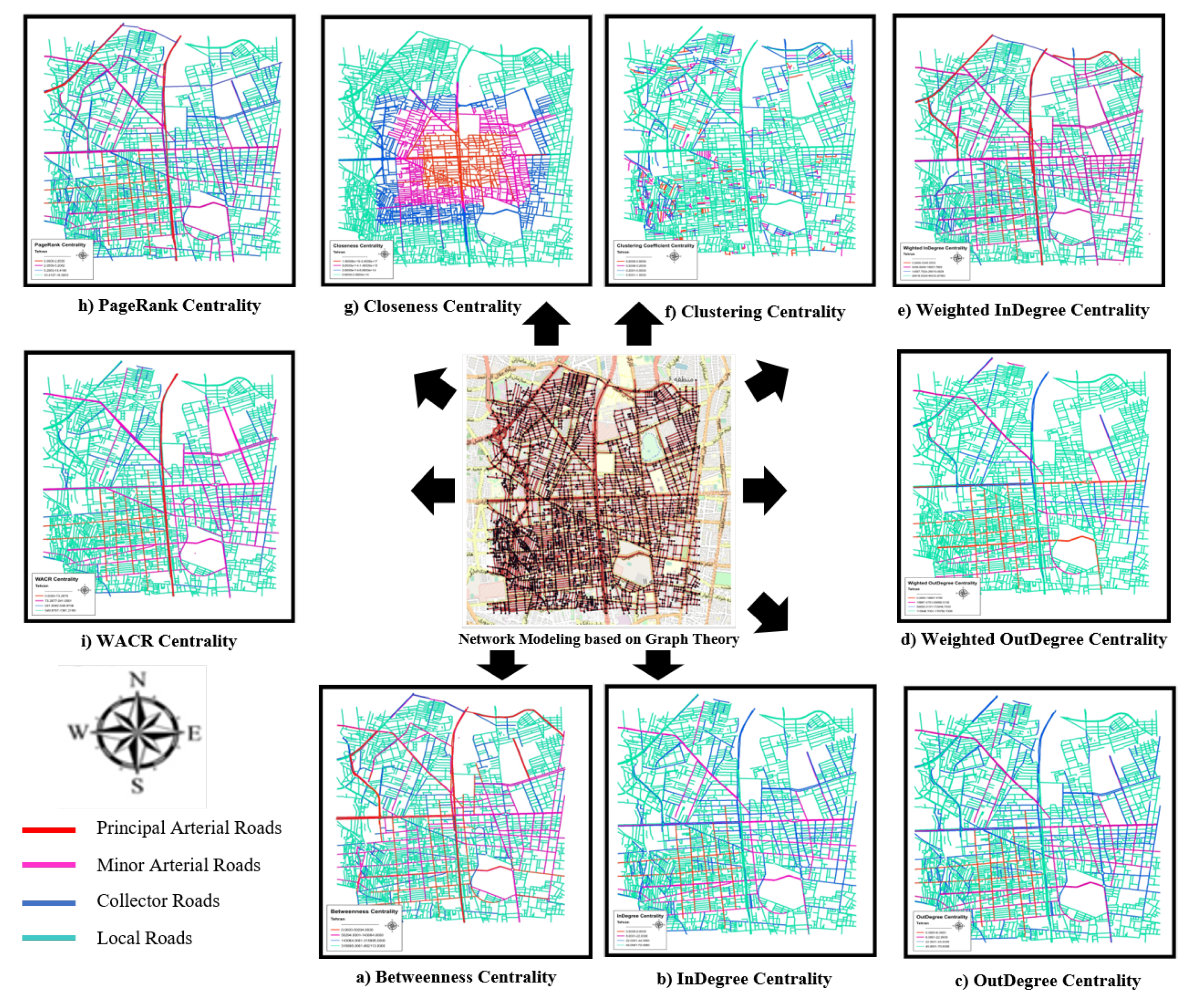
To extract the centrality measures, the main axes of all roads are modeled using the street segment method. This means that the road between two consecutive junctions is considered a separate segment in the network. The modeled street segments were used to construct the strokes. These strokes were constructed using the every best fit method. Street directions were also considered in designing the strokes. In this study, the datasets for four different cities are utilized. The streets for each city are grouped into four classes based on the functionalityL Principal Arterial road (PAr), Minor Arterial road (MAr), Collector road (Cr), and Local road (Lr). For each street, nine different centrality features are determined, and the statistical information of all nine centrality measures has been summarized in Table 1. After preprocessing the data, the structural feature vector is computed for each stroke, then the vectors are normalized to the range of [−1,1]. As a single stroke consists of several street segments with different functionality in the real world, the structural measures of each stroke are assigned to all constituent street segments. Through all of the different machine learning model implementations, 75 % of measures are used for training and 25 % for testing.

3.2. Algorithm Set-Up

We chose four common machine learning models, namely, Logistic Regression (LR), MultiLayer Perceptron (MLP), Support Vector Machines (SVM), and Random Forest (RF), to compare to the proposed SDAE model for use in SFC. Machine learning and deep learning classifiers usually have parameters that need to be set by the user, known as hyperparameters. Hyperparameter tuning involves choosing values for these hyperparameters that result in the optimal performance of a model. The hyperparameters used for each of the traditional machine learning models and our SDAE model are given in Table 2. The hyperparameter values are selected based on the grid-search technique [63] with cross-validation [64]. Each hyperparameter is given a list of discrete values, and for each combination of different hyperparameters, a 5-fold cross-validation training is employed. The data is broken into five equal parts, and each part is used as testing data, while the rest of the data (the other four parts) is used for training, giving 5-fold cross-validation. The set of hyperparameters that achieve the highest classification accuracy are chosen as the hyperparameters to use.
Overfitting is a common problem in all machine learning and deep learning models. Overfitting means the model performed very well on training data but not on test data (unseen data). Regularization is a technique to generalize a model and, in turn, improves the model’s performance on the unseen test data to ameliorate the overfitting problem. Regularization has the same effect on machine learning and deep learning but in different ways. In machine learning, regularization penalizes the coefficients, but in deep learning, it penalizes the weight matrices of the nodes [45].
To design the architecture of the SDAE model we used, a different number of hidden layers and the number of neurons for each layer were tested. The SDAE is trained based on stochastic gradient descent for 75 % of a dataset, and the experiment is repeated 20 times to assess the variability of the process. The trained model is finally evaluated on the test data, the remaining unseen 25 % of a dataset. In this experiment, we vary the number of neurons in the hidden layer from 1–20 to determine the optimum number and also vary the number of hidden layers from two to three. Based on the 95 % confidence interval and standard error estimation for 20 iterations, we end up with the optimum 10 neurons for the first layer and five neurons for a second or bottleneck layer. Generally, for an SAE model there are three ways to control overfitting: adding a penalty term in the loss function (regularization term) to control the weights, adding noise to the input data to force the SAE model to learn more informative features, and sparse decoding by deactivating some of the nodes in each layer randomly. To avoid overfitting, 0– 30 % noise is added to the input data (only the first layer) to satisfy the stacked denoising autoencoder model, and based on the results, 10 % was the optimal value. Moreover, for the regularization term, 0.001 is chosen based on the grid-search technique between the values in the range of 0 to 0.0001 to avoid growing the weights in the deep learning model and overfitting.
LR is a common benchmark machine learning model and is the one simplest used in this work. The regularization term used in the LR model was tested on the range (0.1–10) based on a grid-search strategy to find the optimal value, with 1 chosen. Moreover, to optimize the LR model two different techniques have been tested: SGD and Limited memory Broyden–Fletcher–Goldfarb–Shanno (LBFGS) [65]; LBFGS was the best optimization technique to use in this work. To configure the MLP model, the number hidden layers, the number of neurons per layer, the type of activation function, the optimization technique, and the learning rate are tested in various combinations to find the best configuration for the MLP model. For the LBFGS optimization technique, three hidden layers and 100 neurons for each of them activated by the ReLU activation function were the best hyperparameters for the MLP model. For SVM, an RBF kernel is tested as one of the best kernel methods in kernel-based machine learning models. The values for C, a regularization term, and Gamma as hyperparameters for the RBF kernel were found based on the grid-search strategy: 1 and 10 for C and Gamma, respectively. In this work, RF as one of the best ensemble models has been applied. In the RF training process, there are a two methods to control overfitting: limit the number of nodes per leaf or limit the depth of trees. Based on a grid-search, the optimal values for both of these two hyperparameters for RF were 5 for maximum depth and 4 for the minimum number of nodes per leaf.

3.3. Experimental Results

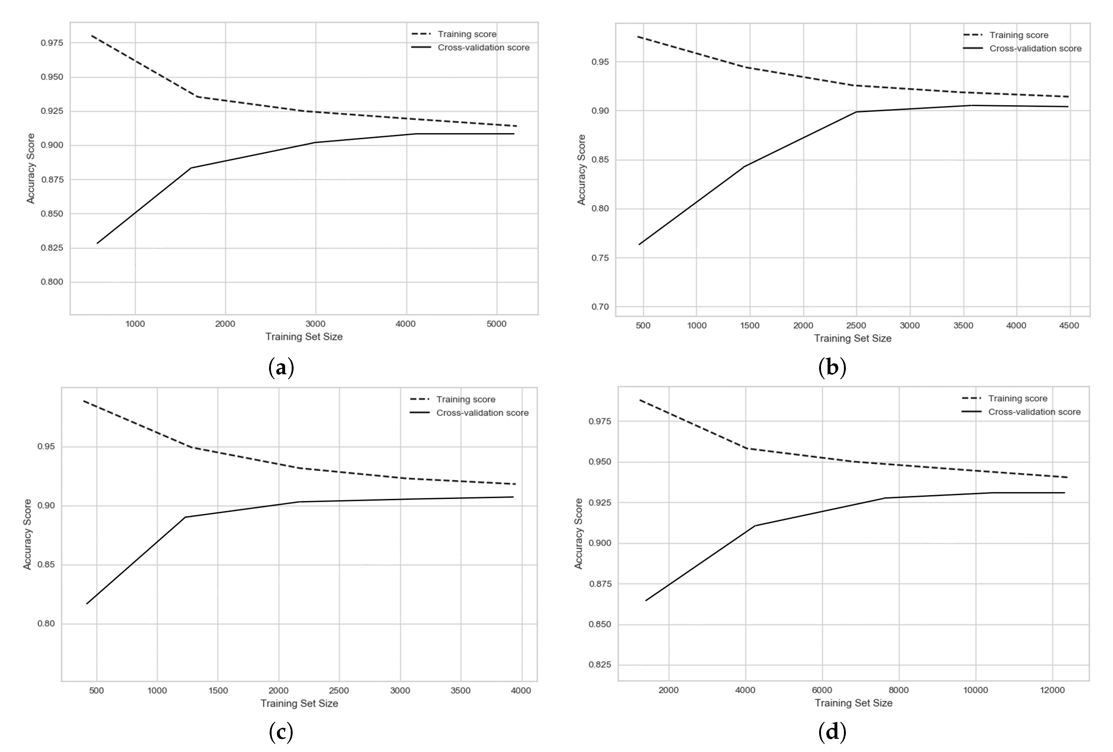
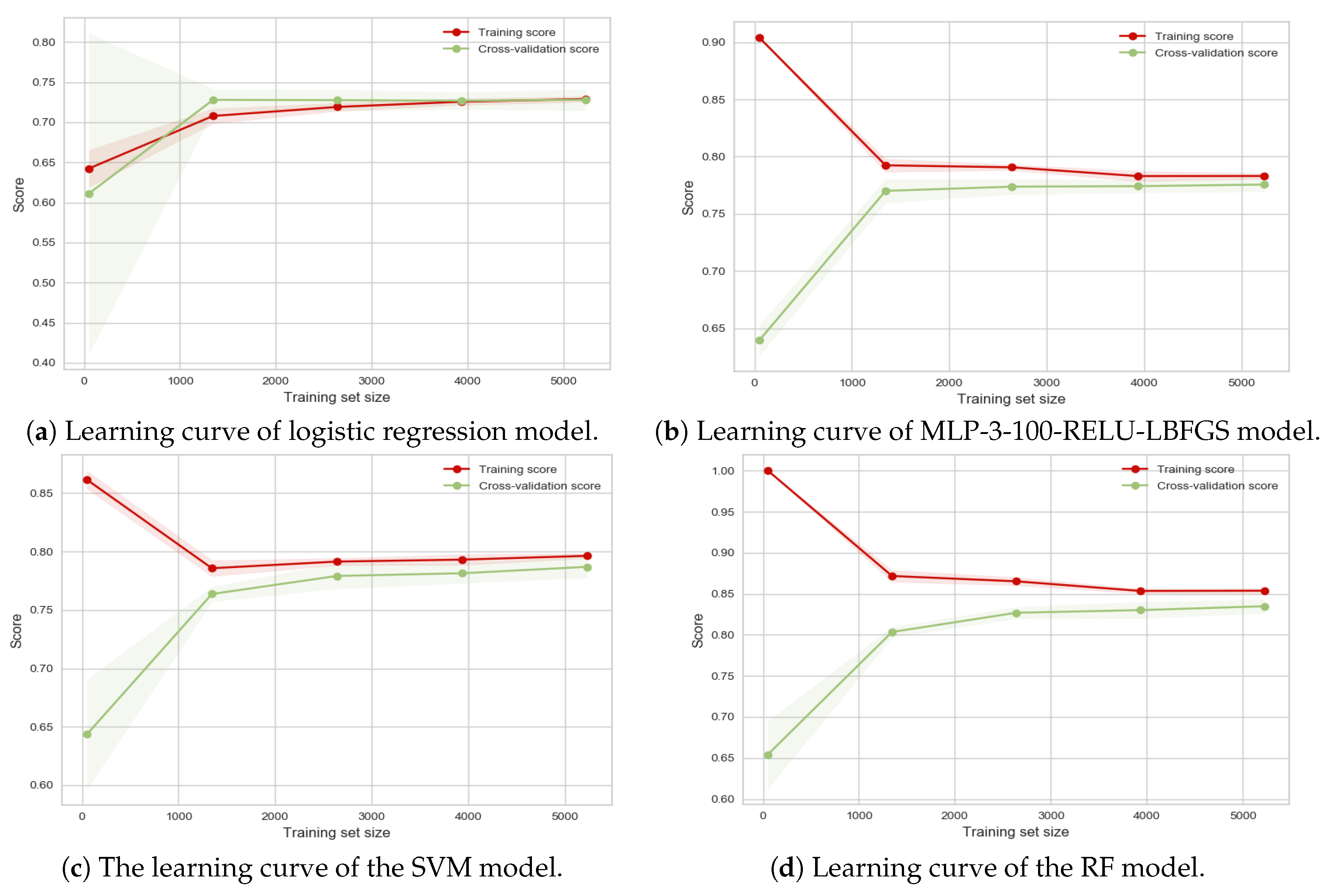
Our proposed SDAE model along with four machine learning models were used to classify the functionality of network streets in four different cities. In this section, the results for all models are shown and discussed. To consider the influence of the amount of input data for different machine learning algorithms and the convergence of the training process, the learning curves for the different models are provided. Each of the input predictors, or the input features, plays a different role and possess a different level of importance on the final performance for a model. In this section, the importance of each input predictor has been considered and discussed. Moreover, the impact of the regularity of the network street and the relationship between regularity of each city on the results of classification is discussed.
Accuracy assessment is an essential step in evaluating the performance and efficiency of different classifiers. In this section, the results of the different implemented models on real data are calculated. To evaluate the performance of the different classifiers, we look at the confusion matrix, R 2 , and Root Mean Squared Error (RMSE). A confusion matrix is a table often used to describe the performance of classification techniques (for more information about the confusion matrix refer to the work in [66]). Overall Accuracy (OA) based on this model is the proportion of the total number of correct predictions. The F-measure metric is based on precision (P) and recall (R) (P is the proportion of the predicted positive cases that were correct and R is the same as true positive), and is calculated as
F 1 = 2 P R P + R
RMSE [67] is regularly employed in model evaluation studies. RMSE provides a complete interpretation of the error distribution in the range of [ 0 , 1 ] , where values close to zero are better. Moreover, to evaluate the best prediction R 2 is used [68], the range of this metric is between [ 0 , 1 ] , where values close to 1 is better. For the rest of the paper, OA for training data is denoted as “OA-Tr”, and OA for the testing dataset as “OA-Te”. Moreover, the F1 score for PAr, MAr, Cr, and Lr classes is denoted as “F1-PAr”, “F1-MAr”, “F1-Cr”, and “F1-Lr”, respectively.
The classification results of our implementation machine learning and deep learning models are presented in Table 3, Table 4, Table 5 and Table 6 for four cities. The results for all datasets reveal that machine learning and deep learning can predict and classify the functionality of the street only based on structural properties of streets. As the results are shown in Table 3, Table 4, Table 5 and Table 6, SDAE has been able to produce more than 90% accuracy of prediction for the training and test sample streets of cities, which are higher than all the proposed models in this experiment.
The overall accuracy for test datasets (OA-Te) is 92 % , 89 % , 92 % , and 92 % for Isfahan, Enschede, Tehran, and Paris, respectively. The results help to infer that the spatial structure of streets plays an important role in forming the functionality of urban roads, because the functionality of streets is detectable by only using structural and spatial properties.
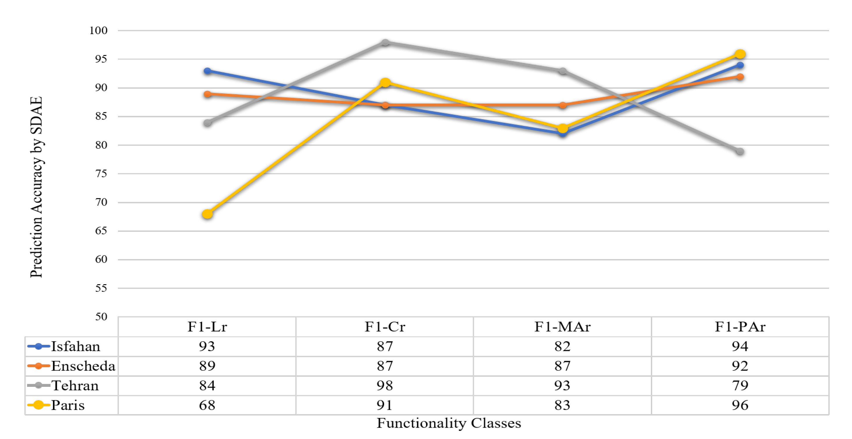
Based on the results of the F1-score proposed for each class of street functionality, it can be stated that every functionality class possessed a specific structural pattern that was distinguishable. The graph depicted in Figure 5 shows the prediction results of the SDAE model for testing sample datasets of each class of street functionality. As shown in the graph, the majority of errors in functionality classes occurred in the most similar classes. Thus, misclassification mostly happens between classes which are similar, rather than between those structurally completely different. For example, misclassification will happen for Cr as Lr classes are structurally and spatially similar and the same for the two classes of primary roads. Figure 5 reveals that the accuracy to detect the class of PAr is higher than MAr and more detectable because spatial properties of MAr’s is very close to PAr, and the same analysis for Cr which has received lower accuracy than Lr.

4. Discussion

In addition to SFC, the impact of regularity of cities on classification, importance of each centrality measure, and the role of deep learning for such a big data processing have been discussed in this section.

4.1. Regularity of Cities and Its Influence on Classification Results

Evaluating the effect of structural patterns on forming the functionality of roads in the real world is very important. It appears that the spatial configuration and structure significantly effects how these patterns are distributed. Different regularity levels in network structures have different impacts on shaping the functionality of urban roads in the real world. To investigate this idea, the level of structural regularity for all cities has been calculated using mixing ratio Equations (10) and (11). Moreover, the classification results are compared with the level of regularity in each network. Figure 6 shows the level of structural regularity (mixing rates) of the cities in the X-axis and their total classification accuracy in the Y-axis.
Based on the results provided in Figure 6 for the overall classification mixing rate for all different cities, it can be concluded that the hierarchical nature of roads in urban areas can also be revealed based on their structural features. According to the results, it can be inferred that in the networks with regular configuration (where the same pattern is repeated in the network), there is a strong relationship between the functionality of a road and its structural properties. In other words, in regular networks like Tehran and Isfahan, which proposed a higher mixing rate and overall accuracy, the spatial structure showed great influence on forming the class of functionality in real-world streets. On the other hand, for cities in this study in which the arrangement of streets is less regular, like Paris or Enschede with less than 72 % mixing rate and less than lower overall accuracy, the existing spatial structure has a lower influence on shaping the street functionalities leading to weak structural patterns in each functionality class. In conclusion, for the case study in the present research, the level of structural regularity in the spatial configuration of urban networks is an effective factor in forming the functionality of urban roads, although more investigation is required in other cities.

4.2. The Importance of Each Centrality Features

Figure 7 presents the importance of the contribution of each feature in the classification for all four test datasets; the horizontal axis indicates the feature and the vertical axis is the percentage of importance. The most important feature for each city is the highest column in the graph. The importance of each feature is calculated based on the concepts of the random forest, as the node impurity weight is decreased by the probability of reaching that node. The node probability is calculated by the number of samples that reach the node, divided by the total number of samples. The higher the value, the more important the feature [69].
Concerning the results in Figure 7, for Paris and Enschede, betweenness is the most important feature, and for Tehran and Isfahan, it is one of the most important features. Generally, this means betweenness is the most important feature in the prediction of street functionality and even the movement patterns. This result reveals that the shortest path plays a pivotal role in finding the destination for people. More crowded streets contribute more to the shortest path in the network, which is the reason for all cities having betweenness as one of the most important features. Due to this fact, calculating the betweenness of streets results in better prediction of the amount of traffic. Calculating betweenness in the network can help to have a better design for new street construction.
After betweenness, weighted in and out-degree is the most important features mostly for Isfahan and Tehran. Street degree (in and out-degree) contributes to having more connections and more applicability in use for people to reach their destination. For Isfahan and Tehran with a higher level of regularity, the importance of betweenness is not the highest due to a high organization and regularity level of the street network and all streets have close contributions to carry traffic. In weighted degrees, streets with higher weights have more connection with Primary Arterial roads, which in such regular cities like Isfahan and Tehran contributed more in the prediction of traffic. Closeness for all the cities in our study has the lowest importance because people mostly driving in the shortest path to their destination, not the roads with higher accessibility and more connections (the closeness definition).

4.3. Deep Learning for Big Data Processing

In this fast-growing scientific world and the enabling of collecting big data, deep learning is playing an important role in big data solutions. Except for having large volume, the large variety and complexity characteristic of big data is a big challenge for shallow neural networks and traditional machine learning. In this work, we applied a large dataset for four cities with high complexity and nonlinearity. The RMSE metric based on linear regression for all datasets is 0.69 , 0.72 , 0.65 , and 0.72 for Isfahan, Enschede, Tehran, and Paris, respectively. These results for linear regression RMSE point out the high nonlinearity of our datasets.
Unlike traditional machine learning and shallow neural networks, deep learning models take advantage of massive nonlinear functions which can learn representation and complexity of features. Most importantly, greedy layer-wise unsupervised learning models such as SDAE can learn latent features (the most important features of input predictors to feed into the classifier) at a higher presentation level. Table 3, Table 4, Table 5 and Table 6 show SDAE outperforming LR and the shallow neural networks: SVM and random forest. In addition, LR is used as a classifier separately to show that the feature generated by SDAE in a higher level of representation are more separable than raw input data and based on our results provided in Table 3, Table 4, Table 5 and Table 6, SDAE+LR worked better than LR as a supervised learning classifier. This is because the SDAE learns the features in a nonlinear manner based on a greedy layer-wise technique and generates new features that are combinations of the existing features, then LR classifies using these new features based on corresponding labeled data.
When we are using machine learning and deep learning models, we want to keep errors as low as possible. There are two major sources of errors for machine learning models: bias and variance. The amount by which the estimation varies as we change the training dataset is called variance, and the bias is the number of errors due to the assumption of linearity of the dataset. To consider the variance and bias of prediction by different models, datasets are split into separate training and validation sets. In this research, the 5-fold cross-validation technique has been used. The learning curve is the best technique to check these two sources of error, which have been depicted for the deep learning models in Figure 8 and all machine learning models for Isfahan in Figure 9. The horizontal axis is the training set size and the vertical axis is accuracy (it can be error instead). The learning curves shown in Figure 8 for the SDAE model show that this model has provided the best results for all cities tested with the best convergence. A good convergence means the algorithm can model the nonlinearity and complexity of the input features, and the algorithm does not need more training samples to understand the behavior of the input features to model.
In Figure 9, the learning curve for all machine learning models for Isfahan is depicted. The model MLP-3-100-RELU-LBFGS has been able to predict but still, there is a low bias problem by providing low accuracy. SVM provided a good convergence condition and good variance but low bias and weakness to predict the complexity and nonlinearity of features. RF models provided higher accuracy with high bias and low variance, but still, there exists a problem where there is a big gap in the middle and even end of two green and red lines, which means this model still needs more data for training the model to converge to a good error rate. Based on the learning curve for the logistic regression model, it is clear that this model has not been able to predict the complexity and nonlinearity of all training features very well. Because, first of all, the accuracy of prediction is not good so the rate of training error is high (low bias problem). Moreover, it seems that this amount of data is a lot for these models because there is no gap between two learning lines at the beginning (high variance problem, a wide area around the line), so these models could not predict the complexity of the input features, and, as we can see, the results are not good either.

5. Conclusions

There have been many studies conducted on understanding the role of spatial structures in the individual movement pattern. The current study provides two new perspectives on a spatial structural study in urban networks. In this study, nine different structural measures were used to examine the spatial structural effect on forming the functionality of urban roads. Different machine learning techniques, such as logistic regression, MLP, SVM, and random forest, alongside a deep learning model called Stacked Denoising Autoencoder, are applied to reveal the patterns existing in each functionality class of urban roads. To achieve this goal, a training set of street segments, defined by their feature vector and functionality class was fed to the different models.
The results show that with an acceptable accuracy provided by SDAE, it is possible to predict the functionality of streets just based on their spatial structural properties. This means that for each real-world functionality class, there exists a specific spatial structural pattern, and the structural properties of streets within a functionality class seem quite similar. It can be concluded that the spatial structure of urban networks is an effective factor in forming the role and importance of each street in the real world. In other words, the structural importance of some urban roads has caused them to be used more frequently than others, which in turn leads to some physical changes in the road’s features to adapt to the high traffic demands. This consequently turns most of these roads to famous roads with high capacity, mostly known as arterial roads. On the other hand, some other roads, because of their spatial positions in city networks, are usually used by fewer passengers; this situation leads to these roads becoming access roads which are known as minor roads.
The classification results also presented a hierarchy that was interestingly similar to the road conceptual hierarchy in the real world. In other words, although this classification was performed by just applying structural properties, its results were arranged exactly in the same way urban roads did. This means that in all functionality classes predicted by machine learning and deep learning models, a majority of errors occurred in the most similar classes. It would be remarkable when we notice that the training dataset did not have any information about the order of functionality classes and the resulted hierarchy in classification has occurred just based on structural properties. Furthermore, the results showed that in regular networks, in which a spatial pattern is repeated in different parts of the city, the deep learning model was able to predict the real-world functionality class more accurately. It implies that in regular networks, there is a prominent spatial structure pattern in each functionality class in comparison with less regular networks. It means that in regular networks, the spatial structures and configurations have a higher impact on forming street roles in the real world. On the other hand, in less regular networks, the significance of spatial structure is reduced in forming street functionality, which in turn produces weak structural patterns in each functionality class in the real world. In conclusion, the level of structural regularity in urban networks is a key factor in forming functionality and the importance of streets in the real world. Furthermore, SDAE demonstrated that for processing big data with nonlinearity and complexity, deep learning models outperform all traditional machine learning and ensemble models.

Author Contributions

Conceptualization, Hamid Kamangir, Fatemeh Noori, Scott A. King, Alaa Sheta, Mohammad Pashaei and Abbas SheikhMohammadZadeh; methodology, Hamid Kamangir, Fatemeh Noori, and Mohammad Pashaei; investigation, H.K., Fatemeh Noori, and Mohammad Pashaei; resources, Fatemeh Noori, Abbas SheikhMohammadZadeh; data curation, Fatemeh Noori, Abbas SheikhMohammadZadeh; writing—original draft preparation, Hamid Kamangir and Fatemeh Noori; writing—review and editing, Scott A. King and Alaa Sheta; visualization, Hamid Kamangir and Scott A. King; supervision, Scott A. King, Alaa Sheta, Abbas SheikhMohammadZadeh; project administration, Hamid Kamangir; funding acquisition Scott A. King. All authors have read and agreed to the published version of the manuscript.

Funding

This research received no external funding.

Conflicts of Interest

The authors declare no conflict of interest.

References

  1. Jiang, B.; Harrie, L. Selection of streets from a network using self-organizing maps. Trans. GIS 2004, 8, 335–350. [Google Scholar] [CrossRef]
  2. Borgatti, S.P. Centrality and network flow. Soc. Netw. 2005, 27, 55–71. [Google Scholar] [CrossRef]
  3. Porta, S.; Crucitti, P.; Latora, V. The network analysis of urban streets: A dual approach. Phys. A Stat. Mech. Its Appl. 2006, 369, 853–866. [Google Scholar] [CrossRef] [Green Version]
  4. Blanchard, P.; Volchenkov, D. Mathematical Analysis of Urban Spatial Networks; Springer Science & Business Media: Berlin/Heidelberg, Germany, 2008. [Google Scholar]
  5. Kazerani, A.; Winter, S. Can betweenness centrality explain traffic flow. In Proceedings of the 12th AGILE International Conference on Geographic Information Science, Hannover, Germay, 2–5 June 2009; pp. 1–9. [Google Scholar]
  6. Jiang, B.; Liu, C. Street-based topological representations and analyses for predicting traffic flow in GIS. Int. J. Geogr. Inf. Sci. 2009, 23, 1119–1137. [Google Scholar] [CrossRef] [Green Version]
  7. Gao, S.; Wang, Y.; Gao, Y.; Liu, Y. Understanding urban traffic-flow characteristics: A rethinking of betweenness centrality. Environ. Plan. B Plan. Des. 2013, 40, 135–153. [Google Scholar] [CrossRef] [Green Version]
  8. U.S. Department of Transportation. Highway Functional Classification: Concepts, Criteria and Procedures; USDoT: Washington, DC, USA, 2013.
  9. Penn, A.; Hillier, B.; Banister, D.; Xu, J. Configurational modelling of urban movement networks. Environ. Plan. B Plan. Des. 1998, 25, 59–84. [Google Scholar] [CrossRef] [Green Version]
  10. Turner, F.C. The Federal-Aid Highway of 1970 and Other Related Bills Prepared for Delivery before the Subcommittee on Roads of the Senate Committee on Public Works. Available online: https://rosap.ntl.bts.gov/view/dot/43207 (accessed on 2 June 2020).
  11. Stamatiadis, N.; Kirk, A.; King, M.; Chellman, R. Development of a context sensitive multimodal functional classification system. Adv. Transp. Stud. 2019, 47, 5–20. [Google Scholar]
  12. Hasan, U.; Whyte, A.; Al Jassmi, H. A Review of the Transformation of Road Transport Systems: Are We Ready for the Next Step in Artificially Intelligent Sustainable Transport? Appl. Syst. Innov. 2020, 3, 1. [Google Scholar] [CrossRef] [Green Version]
  13. Han, B.; Sun, D.; Yu, X.; Song, W.; Ding, L. Classification of Urban Street Networks Based on Tree-Like Network Features. Sustainability 2020, 12, 628. [Google Scholar] [CrossRef] [Green Version]
  14. Xing, H.; Meng, Y. Measuring urban landscapes for urban function classification using spatial metrics. Ecol. Indic. 2020, 108, 105722. [Google Scholar] [CrossRef]
  15. Castro, J.T.; Vistan, E.F.L. A Geographic Information System for Rural Accessibility: Database Development and the Application of Multi-criteria Evaluation for Road Network Planning in Rural Areas. In Urban and Transit Planning; Springer: Berlin, Germany, 2020; pp. 277–288. [Google Scholar]
  16. Sumit, S.H.; Akhter, S. C-means clustering and deep-neuro-fuzzy classification for road weight measurement in traffic management system. Soft Comput. 2019, 23, 4329–4340. [Google Scholar] [CrossRef]
  17. Maeda, K.; Takahashi, S.; Ogawa, T.; Haseyama, M. Convolutional sparse coding-based deep random vector functional link network for distress classification of road structures. Comput.-Aided Civ. Infrastruct. Eng. 2019, 34, 654–676. [Google Scholar] [CrossRef]
  18. Ahmadzai, F.; Rao, K.L.; Ulfat, S. Assessment and modelling of urban road networks using Integrated Graph of Natural Road Network (a GIS-based approach). J. Urban Manag. 2019, 8, 109–125. [Google Scholar] [CrossRef]
  19. Van HIEP, D.; SODIKOV, J. The Role of Highway Functional Classification in Road Asset Management. J. East. Asia Soc. Transp. Stud. 2017, 12, 1477–1488. [Google Scholar]
  20. Zhang, H.; Li, Z. Weighted ego network for forming hierarchical structure of road networks. Int. J. Geogr. Inf. Sci. 2011, 25, 255–272. [Google Scholar] [CrossRef]
  21. Crucitti, P.; Latora, V.; Porta, S. Centrality in networks of urban streets. Chaos Interdiscip. J. Nonlinear Sci. 2006, 16, 015113. [Google Scholar] [CrossRef] [PubMed]
  22. Justen, A.; Martínez, F.J.; Cortés, C.E. The use of space–time constraints for the selection of discretionary activity locations. J. Transp. Geogr. 2013, 33, 146–152. [Google Scholar] [CrossRef]
  23. Zhong, C.; Arisona, S.M.; Huang, X.; Batty, M.; Schmitt, G. Detecting the dynamics of urban structure through spatial network analysis. Int. J. Geogr. Inf. Sci. 2014, 28, 2178–2199. [Google Scholar] [CrossRef]
  24. Berli, J.; Ducruet, C.; Martin, R.; Seten, S. The Changing Interplay Between European Cities and Intermodal Transport Networks (1970s–2010s). In European Port Cities in Transition; Springer: Berlin, Germany, 2020; pp. 241–263. [Google Scholar]
  25. He, S.; Yu, S.; Wei, P.; Fang, C. A spatial design network analysis of street networks and the locations of leisure entertainment activities: A case study of Wuhan, China. Sustain. Cities Soc. 2019, 44, 880–887. [Google Scholar] [CrossRef]
  26. Ližbetin, J. Methodology for determining the location of intermodal transport terminals for the development of sustainable transport systems: A case study from Slovakia. Sustainability 2019, 11, 1230. [Google Scholar] [CrossRef] [Green Version]
  27. Hillier, B.; Penn, A.; Hanson, J.; Grajewski, T.; Xu, J. Natural movement: Or, configuration and attraction in urban pedestrian movement. Environ. Plan. B Plan. Des. 1993, 20, 29–66. [Google Scholar] [CrossRef] [Green Version]
  28. Hillier, B.; Iida, S. Network and psychological effects in urban movement. In Proceedings of the International Conference on Spatial Information Theory, Ellicottville, NY, USA, 14–18 September 2005; Springer: Berlin, Heidelberg, 2005; pp. 475–490. [Google Scholar]
  29. Tsiotas, D.; Polyzos, S. Introducing a new centrality measure from the transportation network analysis in Greece. Ann. Oper. Res. 2015, 227, 93–117. [Google Scholar] [CrossRef]
  30. Ratti, C.; Frenchman, D.; Pulselli, R.M.; Williams, S. Mobile landscapes: Using location data from cell phones for urban analysis. Environ. Plan. B Plan. Des. 2006, 33, 727–748. [Google Scholar] [CrossRef]
  31. Chen, C.; Chen, J.; Barry, J. Diurnal pattern of transit ridership: A case study of the New York City subway system. J. Transp. Geogr. 2009, 17, 176–186. [Google Scholar] [CrossRef]
  32. Kohonen, T. Self-Organizing Maps; Springer Series in Information Sciences; Springer: Berlin, Germany, 2001; Volume 30. [Google Scholar]
  33. Zhou, Q. Selective Omission of Road Networks in Multi-Scale Representation. Ph.D. Thesis, The Hong Kong Polytechnic University, Hong Kong, China, 2012. [Google Scholar]
  34. Wang, P.; Xu, W.; Jin, Y.; Wang, J.; Li, L.; Lu, Q.; Wang, G. Forecasting traffic volume at a designated cross-section location on a freeway from large-regional toll collection data. IEEE Access 2019, 7, 9057–9070. [Google Scholar] [CrossRef]
  35. Lenjani, A.; Dyke, S.J.; Bilionis, I.; Yeum, C.M.; Kamiya, K.; Choi, J.; Liu, X.; Chowdhury, A.G. Towards fully automated post-event data collection and analysis: Pre-event and post-event information fusion. Eng. Struct. 2020, 208, 109884. [Google Scholar] [CrossRef] [Green Version]
  36. Kamangir, H.; Rahnemoonfar, M.; Dobbs, D.; Paden, J.; Fox, G. Deep hybrid wavelet network for ice boundary detection in radra imagery. In Proceedings of the IGARSS 2018-2018 IEEE International Geoscience and Remote Sensing Symposium, Valencia, Spain; 2018; pp. 3449–3452. [Google Scholar]
  37. Pashaei, M.; Kamangir, H.; Starek, M.J.; Tissot, P. Review and Evaluation of Deep Learning Architectures for Efficient Land Cover Mapping with UAS Hyper-Spatial Imagery: A Case Study Over a Wetland. Remote Sens. 2020, 12, 959. [Google Scholar] [CrossRef] [Green Version]
  38. Pashaei, M.; Starek, M.J.; Kamangir, H.; Berryhill, J. Deep Learning-Based Single Image Super-Resolution: An Investigation for Dense Scene Reconstruction with UAS Photogrammetry. Remote Sens. 2020, 12, 1757. [Google Scholar] [CrossRef]
  39. Glorot, X.; Bordes, A.; Bengio, Y. Deep sparse rectifier neural networks. In Proceedings of the Fourteenth International Conference on Artificial Intelligence and Statistics, Fort Lauderdale, FL, USA, 11–13 April 2011; Volume 15 of JMLR. pp. 315–323. [Google Scholar]
  40. Lv, Y.; Duan, Y.; Kang, W.; Li, Z.; Wang, F.Y. Traffic flow prediction with big data: A deep learning approach. IEEE Trans. Intell. Transp. Syst. 2015, 16, 865–873. [Google Scholar] [CrossRef]
  41. Vincent, P.; Larochelle, H.; Lajoie, I.; Bengio, Y.; Manzagol, P.A. Stacked denoising autoencoders: Learning useful representations in a deep network with a local denoising criterion. J. Mach. Learn. Res. 2010, 11, 3371–3408. [Google Scholar]
  42. Koesdwiady, A.; Soua, R.; Karray, F. Improving traffic flow prediction with weather information in connected cars: A deep learning approach. IEEE Trans. Veh. Technol. 2016, 65, 9508–9517. [Google Scholar] [CrossRef]
  43. Lotfollahi, M.; Siavoshani, M.J.; Zade, R.S.H.; Saberian, M. Deep packet: A novel approach for encrypted traffic classification using deep learning. Soft Comput. 2017, 24, 1999–2012. [Google Scholar] [CrossRef] [Green Version]
  44. Lenjani, A.; Dyke, S.; Bilionis, I.; Yeum, C.M.; Choi, J.; Lund, A.; Maghareh, A. Hierarchical Convolutional Neural Networks Information Fusion for Activity Source Detection in Smart Buildings. Struct. Health Monit. 2019. [Google Scholar] [CrossRef]
  45. Hinton, G.E.; Osindero, S.; Teh, Y.W. A fast learning algorithm for deep belief nets. Neural Comput. 2006, 18, 1527–1554. [Google Scholar] [CrossRef]
  46. Haykin, S. Neural Networks: A Comprehensive Foundation; Prentice Hall PTR: Upper Saddle River, NJ, USA, 1994; ISBN 978-0-13-147139-9. [Google Scholar]
  47. Smola, A.J.; Schölkopf, B. A tutorial on support vector regression. Stat. Comput. 2004, 14, 199–222. [Google Scholar] [CrossRef] [Green Version]
  48. Svetnik, V.; Liaw, A.; Tong, C.; Culberson, J.C.; Sheridan, R.P.; Feuston, B.P. Random forest: A classification and regression tool for compound classification and QSAR modeling. J. Chem. Inf. Comput. Sci. 2003, 43, 1947–1958. [Google Scholar] [CrossRef]
  49. Bengio, Y.; Lamblin, P.; Popovici, D.; Larochelle, H. Greedy layer-wise training of deep networks. In Advances in Neural Information Processing Systems; The MIT Press: Cambridge, MA, USA, 2007; pp. 153–160. [Google Scholar]
  50. Hillier, B.; Hanson, J. The Social Logic of Space; Cambridge University Press: Cambridge, UK, 1989. [Google Scholar]
  51. Thomson, R.C.; Richardson, D.E. A graph theory approach to road network generalisation. In Proceedings of the 17th International Cartographic Conference-10th General Assembly of ICA, Barcelona, ES, Spain, 3–9 September 1995; pp. 1871–1880. [Google Scholar]
  52. Chaudhry, O.; Mackaness, W. Rural and Urban Road Network Generalisation: Deriving 1: 250,000 from OS MasterMap; Institute of Geography, The School of Geosciences, The University of Edinburgh: Edinburgh, UK, 2006. [Google Scholar]
  53. Brandes, U. A faster algorithm for betweenness centrality. J. Math. Sociol. 2001, 25, 163–177. [Google Scholar] [CrossRef]
  54. Freeman, L.C. Centrality in social networks conceptual clarification. Soc. Netw. 1978, 1, 215–239. [Google Scholar] [CrossRef] [Green Version]
  55. Opsahl, T.; Panzarasa, P. Clustering in weighted networks Soc. Networks 2009, 31, 155–163. [Google Scholar] [CrossRef]
  56. Brin, S.; Page, L. The anatomy of a large-scale hypertextual web search engine. Comput. Netw. ISDN Syst. 1998, 30, 107–117. [Google Scholar] [CrossRef]
  57. Lovász, L. Random walks on graphs: A survey. Comb. Paul Erdos Is Eighty 1993, 2, 1–46. [Google Scholar]
  58. Lovász, L.; Winkler, P. Mixing of Random Walks and Other Diffusions on a Graph; London Mathematical Society Lecture Note Series; Cambridge University Press: Cambridge, UK, 1995; pp. 119–154. [Google Scholar]
  59. Charte, D.; Charte, F.; García, S.; del Jesus, M.J.; Herrera, F. A practical tutorial on autoencoders for nonlinear feature fusion: Taxonomy, models, software and guidelines. Inf. Fusion 2018, 44, 78–96. [Google Scholar] [CrossRef]
  60. Li, W.; Fu, H.; Yu, L.; Gong, P.; Feng, D.; Li, C.; Clinton, N. Stacked autoencoder-based deep learning for remote-sensing image classification: A case study of African land-cover mapping. Int. J. Remote Sens. 2016, 37, 5632–5646. [Google Scholar] [CrossRef]
  61. Kamangir, H.; Collins, W.; Tissot, P.; King, S.A. Deep-learning model used to predict thunderstorms within 400 km2 of south Texas domains. Meteorol. Appl. 2020, 27, e1905. [Google Scholar] [CrossRef] [Green Version]
  62. Wang, Z.; Bovik, A.C. Mean squared error: Love it or leave it? A new look at signal fidelity measures. IEEE Signal Process. Mag. 2009, 26, 98–117. [Google Scholar] [CrossRef]
  63. Bergstra, J.; Bengio, Y. Random search for hyper-parameter optimization. J. Mach. Learn. Res. 2012, 13, 281–305. [Google Scholar]
  64. Fushiki, T. Estimation of prediction error by using K-fold cross-validation. Stat. Comput. 2011, 21, 137–146. [Google Scholar] [CrossRef]
  65. Zhu, C.; Byrd, R.H.; Lu, P.; Nocedal, J. Algorithm 778: L-BFGS-B: Fortran subroutines for large-scale bound-constrained optimization. ACM Trans. Math. Softw. (TOMS) 1997, 23, 550–560. [Google Scholar] [CrossRef]
  66. Story, M. and Congalton, R.G. Accuracy assessment: A user’s perspective. Photogramm. Eng. Remote. Sens. 1986, 52, 397–399. [Google Scholar]
  67. Chai, T.; Draxler, R.R. Root mean square error (RMSE) or mean absolute error (MAE)?–Arguments against avoiding RMSE in the literature. Geosci. Model Dev. 2014, 7, 1247–1250. [Google Scholar] [CrossRef] [Green Version]
  68. Cameron, A.C.; Windmeijer, F.A. An R-squared measure of goodness of fit for some common nonlinear regression models. J. Econom. 1997, 77, 329–342. [Google Scholar] [CrossRef]
  69. Louppe, G.; Wehenkel, L.; Sutera, A.; Geurts, P. Understanding variable importances in forests of randomized trees. In Advances in Neural Information Processing Systems 26, Proceedings of the Neural Information Processing Systems (NIPS), Lake Tahoe, Nevada, 5–8 December 2013; Neural Information Processing Systems Foundation, Inc.: San Diego, CA, USA; pp. 431–439.
Figure 1. Functional classes of the urban street network in four different cities.
Ijgi 09 00456 g001
Figure 2. Schematic of or our system that performs street functionality classification based on centrality measures using a deep learning model.
Ijgi 09 00456 g002
Figure 3. All nine centrality measures generated for Tehran, Iran.
Ijgi 09 00456 g003
Figure 4. (a) The basic structure of an autoencoder includes an input x, which is mapped onto the encoding y via an encoder (function f). This encoding is in turn mapped to the reconstruction r by means of a decoder (function g). (b) The structure of the Stacked Denoising Autoencoder (SDAE) used in this work.
Ijgi 09 00456 g004
Figure 5. SDAE F1-score of functionality of each class.
Ijgi 09 00456 g005
Figure 6. The mixing rate of cities’ regularity versus SDAE overall accuracy.
Ijgi 09 00456 g006
Figure 7. Importance of features for (a) Isfahan, (b) Enschede, (c) Tehran, and (d) Paris.
Ijgi 09 00456 g007
Figure 8. Learning Curves for SDAE model: (a) Isfahan, (b) Enschede, (c) Tehran, and (d) Paris.
Ijgi 09 00456 g008
Figure 9. Learning curve of machine learning models for Isfahan.
Ijgi 09 00456 g009
Table 1. Statistical summary of centrality measure data for all cities.
Feature Name BetweennessInDegreeWeightInDegreeOutDegreeWeightOutDegreeClusteringWACRPage RankCloseness
Count
Isfahan871187118711871187118711871187118711
Tehran658865886588658865886588658865886588
Enschede748374837483748374837483748374837483
Paris20,69720,69720,69720,69720,69720,69720,69720,69720,697
Mean
Isfahan89,3009.373363.289.3714040.490.0575.302.923.22 × 10 15
Tehran80,876.8812.647088.2312.6322,891.340.05129.113.191.66 × 10 15
Enschede53,698.255.992662.786.036075.360.1338.911.701.51 × 10 15
Paris246,0009.165418.659.392.21 × 10 4 0.18104.122.541.19 × 10 16
STD
Isfahan192,00012.185136.0712.1851,482.610.17211.423.481.91 × 10 16
Tehran131,445.5016.709977.2516.6246,264.950.15279.183.857.90 × 10 15
Enschede112,209.455.852898.235.9815,345.660.2195.021.461.35 × 10 16
Paris419,00012.306694.8013.161.00 × 10 5 0.23525.523.255.34 × 10 16
Min
Isfahan0.000.000.000.000.000.000.000.002.20 × 10 15
Tehran0.000.000.000.000.000.000.000.001.90 × 10 15
Enschede0.000.000.000.000.000.000.000.324.00 × 10 14
Paris0.000.000.000.000.000.000.000.007.70 × 10 15
Max
Isfahan1,670,00069.0036,490.8669.00423,000.001.001756.7512.003.61 × 10 17
Tehran662,113.0072.0049,335.8770.00176,792.701.001361.2216.002.44 × 10 17
Enschede783,939.0038.0013,336.2139.00111,360.201.00746.4110.222.57 × 10 17
Paris5,580,000105.0038,784.84115.001.24 × 10 6 1.006622.5229.517.71 × 10 17
Table 2. Hyperparameters used for each algorithm and the potential values used in the grid search.
AlgorithmHyperparameterValue
LRRegularization, C 0.1 , 1.0 , 10
Optimization functionLBFGS
Iteration Number1000
MLPHidden Layer size2–3
Hidden Layer neurons20–100
Activation FunctionRelu, Logistic
Optimization functionLBFGS, SGD
Momentum 0.9
Learning Rate 0.001
Alpha 0.01
Beta 0.9
Iteration Number1000
SVMRegularization, C 0.1 , 1.0 , 10
KernelRBF
Gamma10
Iteration Number1000
RFNumber of estimators1000
Max-Depth5–10
Min leaf per node2–8
SDAENumber of Hidden Layer2–3
Number of neurons2–15
Regularization 0.1 , 0.001 , 0.0001
Noise Mask0–30%
Table 3. Classification results for Isfahan.
AlgorithmR2RMSEOA-TrOA-TeF1-LrF1-CrF1-MArF1-PAr
Logistic Regression 0.40 0.62 0.73 0.74 0.69 0.55 0.33 0.86
MLP-3-100-ReLU-LBFGS 0.48 0.51 0.77 0.77 0.84 0.66 0.47 0.86
SVM 0.51 0.51 0.79 0.78 0.87 0.66 0.48 0.86
Random Forest 0.73 0.27 0.86 0.84 0.88 0.86 0.78 0.89
SDAE 0.82 0.16 0.92 0.92 0.93 0.87 0.82 0.94
Table 4. Classification results for Enschede.
AlgorithmR2RMSEOA-TrOA-TeF1-LrF1-CrF1-MArF1-PAr
Logistic Regression 0.33 0.56 0.66 0.68 0.38 0.52 0.62 0.79
MLP-3-100-ReLU-LBFGS 0.60 0.35 0.78 0.77 0.74 0.74 0.71 0.82
SVM 0.59 0.37 0.75 0.76 0.67 0.71 0.72 0.82
Random Forest 0.75 0.21 0.83 0.81 0.81 0.84 0.80 0.85
SDAE 0.83 0.15 0.90 0.89 0.89 0.87 0.87 0.92
Table 5. Classification results for Tehran.
AlgorithmR2RMSEOA-TrOA-TeF1-LrF1-CrF1-MArF1-PAr
Logistic Regression 0.40 0.31 0.69 0.70 0.45 0.71 0.70 0.33
MLP-3-100-ReLU-LBFGS 0.54 0.24 0.77 0.77 0.80 0.89 0.79 0.45
SVM 0.51 0.26 0.76 0.76 0.68 0.86 0.79 0.49
Random Forest 0.73 0.13 0.83 0.82 0.83 0.86 0.88 0.58
SDAE 0.83 0.09 0.93 0.92 0.84 0.98 0.93 0.79
Table 6. Classification results for Paris.
AlgorithmR2RMSEOA-TrOA-TeF1-LrF1-CrF1-MArF1-PAr
Logistic Regression 0.08 0.7 0.66 0.67 0.10 0.62 0.05 0.86
MLP-3-100-ReLU-LBFGS 0.13 0.81 0.76 0.74 0.15 0.57 0.20 0.85
SVM 0.19 0.87 0.73 0.70 0.20 0.53 0.29 0.80
Random Forest 0.52 0.37 0.84 0.83 0.52 0.82 0.62 0.92
SDAE 0.79 0.16 0.94 0.92 0.68 0.91 0.83 0.96

