Change Detection in Multispectral Remote Sensing Images with Leader Intelligence PSO and NSCT Feature Fusion

Abstract

Change detection (CD) using Remote sensing images have been a challenging problem over the years. Particularly in the unsupervised domain it is even more difficult. A novel automatic change detection technique in the unsupervised framework is proposed to address the real challenges involved in remote sensing change detection. As the accuracy of change map is highly dependent on quality of difference image (DI), a set of Normalized difference images and a complementary set of Normalized Ratio images are fused in the Nonsubsampled Contourlet Transform (NSCT) domain to generate high quality difference images. The NSCT is chosen as it is efficient in suppressing noise by utilizing its unique characteristics such as multidirectionality and shift-invariance that are suitable for change detection. The low frequency sub bands are fused by averaging to combine the complementary information in the two DIs, and, the higher frequency sub bands are merged by minimum energy rule, for preserving the edges and salient features in the image. By employing a novel Particle Swarm Optimization algorithm with Leader Intelligence (LIPSO), change maps are generated from fused sub bands in two different ways: (i) single spectral band, and (ii) combination of spectral bands. In LIPSO, the concept of leader and followers has been modified with intelligent particles performing Lévy flight randomly for better exploration, to achieve global optima. The proposed method achieved an overall accuracy of 99.64%, 98.49% and 97.66% on the three datasets considered, which is very high. The results have been compared with relevant algorithms. The quantitative metrics demonstrate the superiority of the proposed techniques over the other methods and are found to be statistically significant with McNemar’s test. Visual quality of the results also corroborate the superiority of the proposed method.

1. Introduction

Change detection (CD) is the process of identifying changes occurred at a scene between two time points, using multi-temporal images. It is an active research area due to its numerous applications in real-life [1,2,3,4]. In this paper, the focus is on remote sensing change detection [2,5], owing to the following aspects. Firstly, monitoring large area is possible with satellite imageries, which otherwise, is very time consuming and expensive or even not possible due to remote areas [3,6]. Secondly, quick and automated systems to monitor changes are extremely necessary for deploying timely actions in various realistic problems such as disaster management/assessment, monitoring land use/land cover changes or forest cover changes due to fire/infestations, urbanization and environmental monitoring, and oceanography [4,6,7,8,9]. Though we find a profusion of CD techniques in the literature, most of these methods are application specific and highly depend on the spectral, spatial and sensor characteristics of the imageries used and cannot be considered as optimal [1,6,7,10,11,12,13,14,15,16,17,18,19,20]. In addition to that, they often fail to address the real challenges while the dynamics occurred is complex or heterogeneous in nature. As multispectral remote sensing images depict the signature of various land cover types better in one band than other, powerful techniques to derive CD map by drawing information from multiple spectral bands are the need of the hour.

For the remote sensing problems, getting a proper ground truth is difficult in many situations. Therefore, unsupervised methods are preferred to supervised methods, as this does not require learning with training patterns [3,21,22]. Generally, the change detection in unsupervised framework consists of three steps: preprocessing, image comparison and image analysis [1,3]. In the preprocessing step, anomalies due to radiometric and geometric factors [23,24] are removed by correction algorithms and georeferencing, respectively. Noise trapped in the images is also filtered out to some extent in this stage for improving the strength of the signals. And the two images (captured at different dates) are co-registered by providing the pixel-to-pixel alignment, before computing the difference images.

From the rectified images, difference image (DI) is generated in the second step, usually by subtraction or ratioing [1,22,24,25]. While the former calculates the difference in intensity values of pixels between the images at two dates, the latter computes the ratio of corresponding pixels [24,26]. In the ratio image, the changed pixels are aligned away from “1” unsymmetrically on both sides, where the value “1” corresponds to the unchanged pixel, as equal values produce 1 on ratioing [1,2]. By the hypothesis of few changes between the images of two times, changes can be detected in the tails of the statistical distribution of the pixel values in the difference image [22]. Another widely used method is change vector analysis (CVA) computed from multiple spectral bands [3,6,23]. The CVA and subtraction method have been used in change detection of various geographical environments [1,6,25] but researchers argue that it is too simple to deal with all complexities involved in detecting the real changes on various land covers [1,6,23,25]. Moreover, they are not robust against noise and effects due to external factors [6]. Whereas ratioing is efficient in inhibiting the effects of slope, sun angle and illumination variations and has been employed in a wide variety of CD problems [25], but its nonlinear nature is much criticized [22,25]. The two methods, subtraction and ratioing, are simple and easy to implement, have demonstrated exclusive behaviour on different land cover types [1,24,25]; that is, ratio method is good for detecting changes in water, soil and urban scene; difference method is good for detecting vegetation and water [24,25]; hence, they can be complementary to some extent.

As the accuracy of change map has a strong bias on the quality of the difference images (DI), fusion techniques [7,13,27] are often adopted to enhance the quality of DI, at pixel level or in transform domain [7,13,28]. Therefore, in the present study, we propose fusion of a normalized difference image (NDI) and a normalized ratio image (NRI) to produce a better quality difference image, in the Nonsubsampled Contourlet Transform (NSCT) [29] domain by exploiting the distinct properties of NSCT such as shift and scale invariance and multidirectional frequency localizations [30].

In the final step, the DI is partitioned into two groups, changed or unchanged, using a suitable technique, such as thresholding or segmentation [7,10,24,31]. The choice of proper threshold has always been challenging [23,26,32,33]; hence, the use of classification/clustering algorithms became popular [6,7,26]. Acquiring accurate labeled data is crucial for getting good classification results which is very difficult or even impossible in the case of remote sensed data [3,26]. So, clustering algorithms received much attention from researchers in recent years as these algorithms can derive clusters independently [3,24,26]. Hard clustering algorithms like K-means and ISODATA that produce crisp clusters have been applied in many CD studies [3,26,34]. However, for remote sensing images (where pixels belong to overlapping clusters), fuzzy clustering techniques that generate clusters based on the degree of membership of pixels are found to be more appropraite [3]. Several variants of fuzzy algorithms that incorporate spatial information to increase the accuracy of change detection have been reported in the literature [3,7,13,14,35].Techniques such as multi-resolution Markov random field models [15], random walks [10] and hybrid methods like hybrid conditional random field [12], Markov-CA Model [18,36], Kmeans clustering with Adaptive majority voting [37] are also into great interest now. When employing optimization techniques on clustering algorithms, the accuracy of change detection is found to be improved further [35,38]. Nature inspired algorithms such as Particle Swarm Optimization (PSO) [39], Firefly Algorithm [40], Ant Colony Optimization (ACO) [41] and so forth are powerful techniques that can be used for solving complex problems by utilizing the metaheuristics underlying the nature, for example, swarm intelligence [42,43]. Due to its simplicity and nominal parameters, PSO was investigated thoroughly and has been applied in several real world problems including change detection [42,43,44,45]. However, PSO has two major shortcomings: early convergence or no convergence, and menace of local optima [42,43] due to loss of diversity of particles after a few iterations. We address these issues in the proposed PSO variant, called Leader Intelligence PSO (LIPSO). In LIPSO, an intelligent Leader [46] and the followers take Lévy flight [43] occasionally to overcome the local optima problem and thereby the convergence is ensured.

The contributions can be summarized as follows:

• A modified PSO called LIPSO, is proposed to detect the changes in the remote sensing images.
• For the better estimations of the changed regions, three strategies are used: (a) fusing Normalized difference image and Normalized ratio image in the NCST domain, band-wise to generate an improved difference image (b) NSCT decomposition helped in enhancing the information and removing the noise, and (c) tested with different combinations of band-wise difference images with LIPSO to find the best result, and finally, it has been found that all the four bands are equally useful for the detection of the changes.
• An improved version of Change Vector Analysis (CVA) [3], named Transform CVA, is proposed.
• The proposed method is compared with Fuzzy C means (FCM) [3], Standard PSO (SPSO) [47], PSO with Lévy flight (PSOLF) [42,43] and Transform CVA are compared.

The rest of the paper is organized into following sections. In Section 2, the proposed methodology is described in details. In Section 3, the data sets and accuracy metrics are provided. The experimental setup and findings are presented in the Section 4 with detailed analysis of the results. Finally, the conclusion is outlined in Section 5.

2. Materials and Methods

Our objective is to detect the changes occurred from the temporal images by delineating the changed pixels from the unchanged ones. Therefore, the problem is a clustering problem that groups the image pixels into changed and unchanged clusters. Consider two co-registered remote sensing images of intensity values, with B bands $I_1\left(x\right)=\{I_{1,b}(i,j),1<i<M,1<j<N,b=1,2,\dots B\}$ and $I_2\left(x\right)=\{I_{2,b}(i,j),1<i<M,1<j<N,b=1,2,\dots B\}$ acquired at two dates $T_1$ and $T_2$ respectively, of the same geographical area. We process the images to produce a binary change map $\mathcal{G}\left(x\right):\mathcal{R}\to [0,1]$ by segmentation, according to the following rule:

$$\mathcal{G}\left(x\right)=\left\{\begin{array}{cc}0\hfill & \mathrm{if}x\mathrm{belongs}\mathrm{to}\mathrm{changed}\mathrm{region},\hfill \\ 1\hfill & \mathrm{if}x\mathrm{belongs}\mathrm{to}\mathrm{unchanged}\mathrm{region}.\hfill \end{array}\right.$$

For this, we propose a novel change detection technique which focuses on two aspects: the quality of the difference image and the robustness of the segmenting algorithm, which are directly related to the performance of any CD technique. Apparently, it consists of two parts, (i) Generate good quality difference image by NSCT feature extraction and intra-scale fusion, and (ii) Generate binary change map using Leader Intelligence PSO (LIPSO). The workflow of the procedure is shown in the Figure 1.

2.1. Generate Good Quality Difference Image by NSCT Feature Extraction and Intra-Scale Fusion

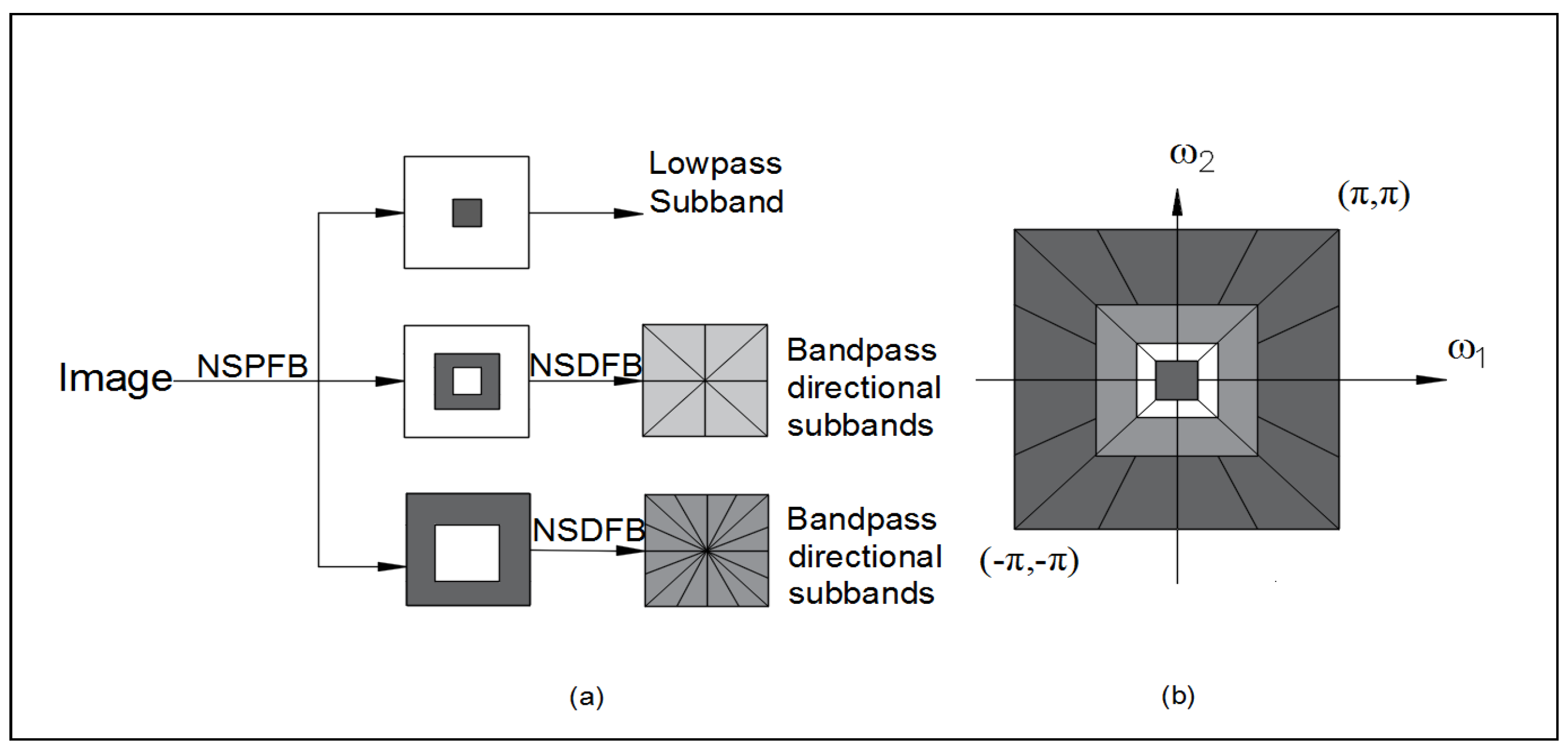
As mentioned in the introduction, fusion of images can produce better quality images, by combining information from multiple source images. Image fusion in transform domains [7,13,28] produces better results as the wavelet/contourlet transforms can represent frequencies in time and space. Nonsubsampled Contourlet Transforms (NSCT) possess advantages such as shift and scale invariance [29], a property more suitable for the change detection studies. Added to that, being multi directional, the NSCT is efficient in capturing 2D singularities [30] to derive edge and line features of image, thus geographical structures in them, while wavelets can capture only point singularities. This transform contains a pair of filter banks, of which, the nonsubsampled pyramidal filter bank (NSPFB) generates sub band pyramids with $j+1$ redundancy at jth scale. The nonsubsampled directional filter bank (NSDFB) produces $2^{l_j}$ directional subbands at $l_j$ level and jth scale [29] resulting into sub bands of multiple coarseness and directions. The structure of the NSCT is illustrated in the Figure 2. 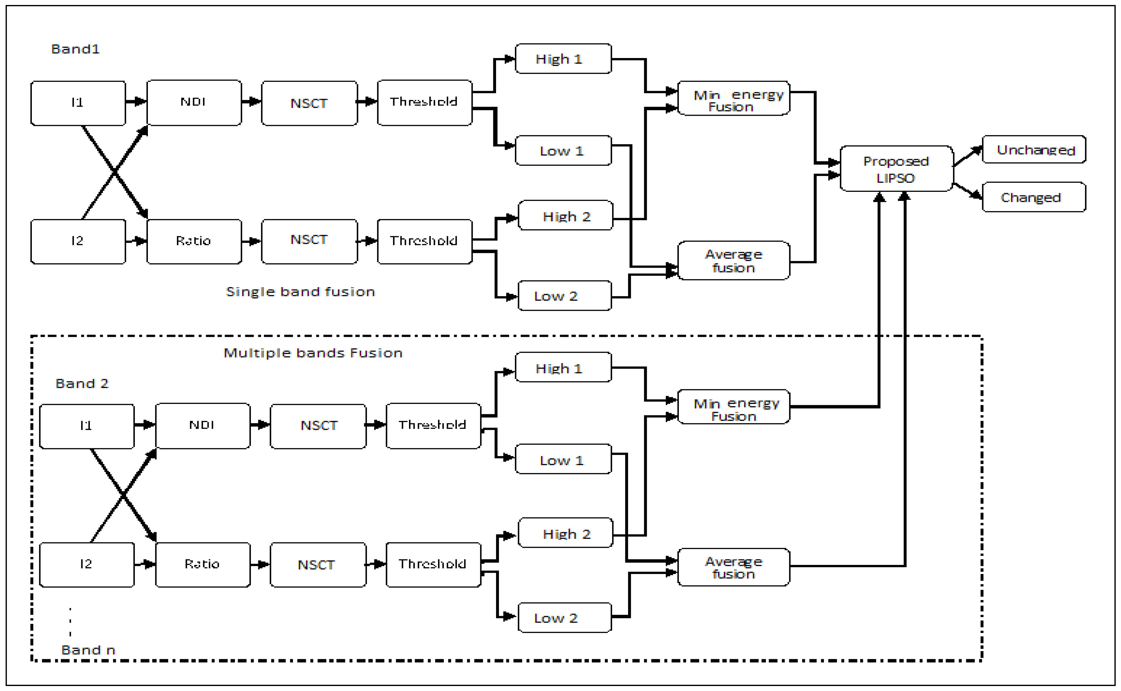A large number of coefficients are zeroes [30] and hence, nonsubsampled contourlets are efficient in suppressing background and various noise models, and can project changed pixels more prominently. In the present study, a NDI and a NRI having complementary information are fused at NSCT feature level, due to their unique properties described earlier and produces fused NSCT coefficients that contain information from the two DI’s mentioned. The steps of the method are summarized in Algorithm 1.

Algorithm 1 NSCT Fusion

Input: Source images $I_1$ at time $T_1$ and $I_2$ at time $T_2$

Output: Fused NSCT coefficients 1: Generate NDI using Equations (1) and (2). 2: Generate NRI using Equation (3). 3: Apply NSCT on the NDI and NRI up to sufficient scales J and obtain approximation coefficients and directional features. 4: Denoise features using appropriate threshold ($\lambda$). 5: Fuse the approximation coefficients by averaging, and high frequency coefficients on minimum energy rule.

The DI by subtraction from spectral bands are generated as

$$D{I}_b=|I_{1,b}-I_{2,b}|$$

(1)

and normalized, called Normalized Difference Image (NDI), as

$$D{I}_b^{nor}\left(NDI\right)=\frac{D{I}_b-D{I}_{b,min}}{D{I}_{b,max}-D{I}_{b,min}},$$

(2)

where $D{I}_{b,max}$ is the maximum pixel value and $D{I}_{b,min}$, the minimum value of pixel (where $b=1,2,\dots ,B$). The second DI, Ratio image is generated as

$$D{I}_b^r\left(NRI\right)=\left|1-\frac{\left(I_{1,b}\right)}{\left(I_{2,b}\right)}\right|.$$

(3)

In the ratio images, as the unchanged pixel will have a value closer to the “1”, we will subtract the values from “1” and take the absolute value to map the values in the range $[0,1]$ (to match with the NDI), we call this as NRI (normalized ratio image). NSCT Features are extracted from these DIs (NDI and NRI) by applying J-scale decompositions (where J-scale is chosen using entropy of the decomposed images). The subband coefficients are denoised using a threshold defined by Donoho and Johnstone equation $\lambda =\sigma \sqrt{2log\left(MN\right)}$ (here, $\sigma$ is estimated suitably and MN is the size of the image) [48]. A large number of background pixels are removed on thresholding and hence, the foreground containg the changed pixels gets enhanced. The resultant sub band contains different land cover information from both NDI and NRI features. The denoised approximation coefficients of NDI and NRI are fused by averaging to produce a resultant sub band comprising of the details of both the $DI$’s equally [7]. The minimum local energy fusion rule is applied on higher frequency sub bands [7] so as to preserve the edge & salient features, using

$$D{H}_{j,b}^{q,f}=\left\{\begin{array}{c}D{H}_{j,b}^{q,nor},E_{j,b}^{q,nor}<E_{j,b}^{q,r}\hfill \\ D{H}_{j,b}^{q,r}\mathrm{otherwise},\hfill \end{array}\right.$$

(4)

where $D{H}_{j,b}^{q,f},D{H}_{j,b}^{q,nor},D{H}_{j,b}^{q,r}$ are high frequency coefficients in direction q at jth scale of fused image, NDI and NRI, and $E_{j,b}^{q,nor},E_{j,b}^{q,r}$ represents the local energy of the coefficient in the direction q of band b at jth scale around $3\times 3$ window of NDI and NRI, respectively.

From each spectral band, ‘S’ number of NSCT features (subband images) of size $M\times N$ each, are obtained after intra-scale fusion, which are mapped to S dimensional vector with respect to each pixel, and segmented by employing the proposed LIPSO algorithm.

2.2. Generate Binary Change Map Using Leader Intelligence PSO

As our task is to produce two mutually exclusive clusters of changed and unchanged pixels, the inter-distance between the clusters is to be maximized and the intra-distance of the pixels in a group is to be minimized. Therefore, this problem can be formulated as an optimization problem trying to minimize the following error function:

$$min\frac{1}{K}\sum _{k=1}^K\sum _{j=1,x_j\in {\mathcal{C}}_k}^{n_k}d(x_j-v_k),$$

(5)

where K is the number of clusters(regions), $x_j$ is the data point belongs to kth cluster(${\mathcal{C}}_k$), $v_k$ is the cluster centre of kth cluster, $d(x_j-v_k)$ is the Euclidean norm and $n_k$ is the number of data points belonging to the kth cluster(region). Particle Swarm Optimization algorithm (PSO) proposed by Kennedy and Eberhart [39,49] is a population based algorithm that imitates the best characteristics of social insects, in solving complex optimization problems [42,43,50]. It is a typical optimization algorithm suitable for realistic problems like clustering and we choose this due to its many virtues: it is a widely accepted optimization method with a well-defined mathematical foundation, especially, when it is combined with Lévy flights [42,43]. Interested readers may please refer to Reference [50] for the theoretical details of PSO and Lévy flight in References [42,43] & in the Appendix A. The metaheuristic underlying in nature such as swarm intelligence is used in PSO for fast convergence of the problem, which is exploited in generating changed and unchanged clusters in our experiment. It is rather easy to understand its logic, require a few parameter settings only and computational overhead is low as compared to many other algorithms.

Despite several variants of PSO are reported in the literature, the local optima problem could not be eliminated completely. Moreover, they often fail in arriving at consistent solution. Of the several improved versions of PSO, the Lévy flight version is found promising. We consider two variants of that, the LFPSO [42] in which the Lévy flight is performed only when the particle exceeds a limit value and the PSOLF [43], where the particles fly according to a probability, $p>0.5$. Although they perform well with benchmark problems [43], they fail to achieve good results in real-life problems like image segmentation resulting into bad clusters or not even generating clusters. It is probably due to the inability of the particles to attain sufficient velocity or fail to maintain a velocity within the search space. A second reason may be due to loss of diversity that leads to stagnation of particles. 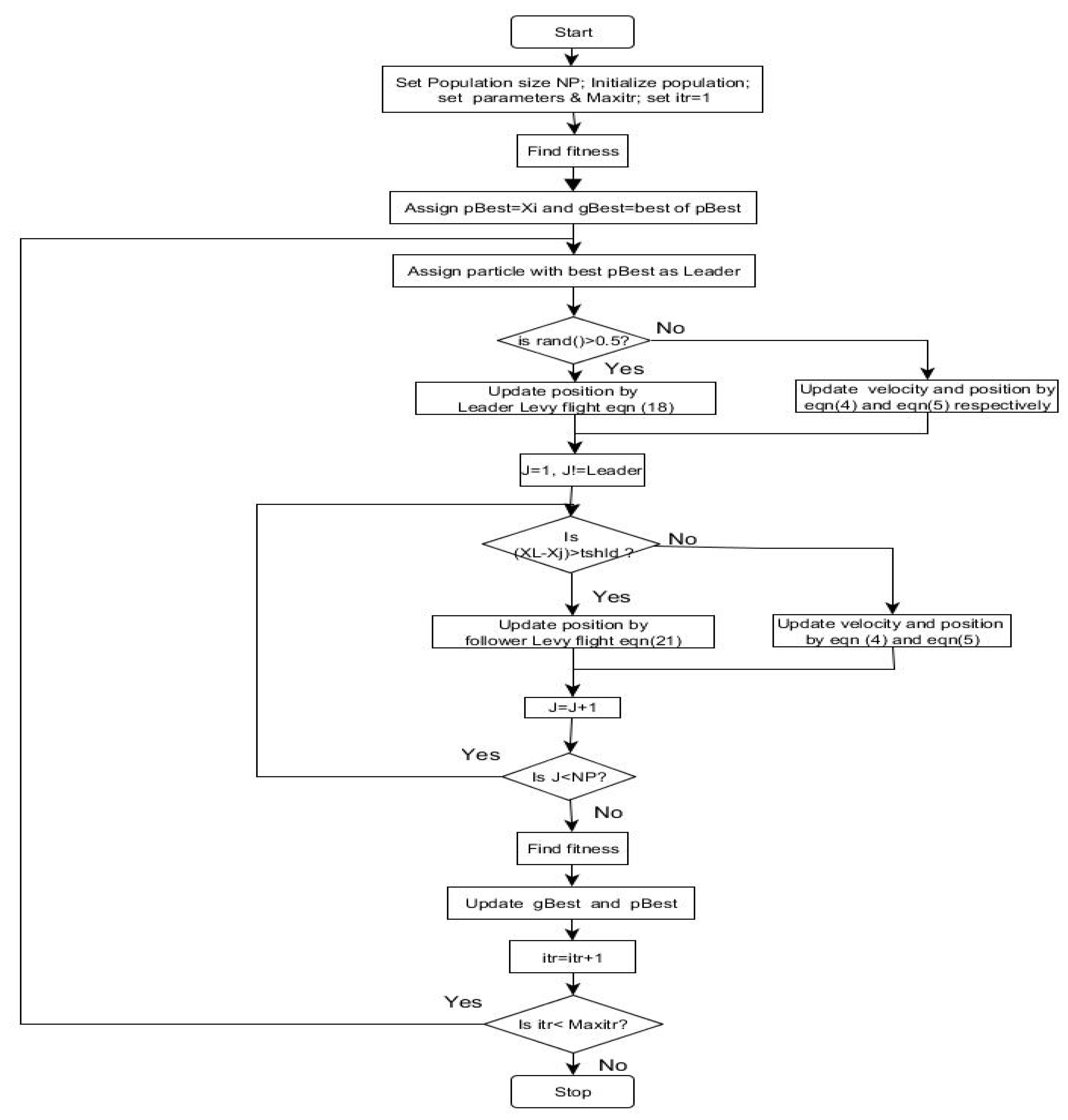Therefore, a modified PSO with the concept of Leader and followers [46] performing Lévy flight intelligently (LIPSO), is proposed. One can easily understand the steps involved in LIPSO from Algorithm 2 and the flowchart in Appendix B.

Algorithm 2 Leader Intelligence Particle Swarm Optimization

Input: Fused coefficients Output: Cluster centres 1: Initialize particles randomly selected from the search space, as $X_i=\{X_{i1},X_{i2},\dots ,X_{iD}\}$. 2: Initialize various parameters: $c_1$ and $c_2$, $Xmax$, $Xmin$, $Vmax$ and $Vmin$. 3: Evaluate fitness by Equation (5). 4: Assign $pBes{t}_{i,D}$ = initial positions of particles, $gBes{t}_D$ = best particle position of swarm, $pBestfi{t}_i$ = the fitness value of ith particle, and $gBestfit$ = the best fitness of the swarm. 5: Set the particle with the highest fitness value as the Leader. 6: If $rand>0.5$ then update position of Leader by Lévy flight using Equation (9), else update velocity and position of Leader by Equations (6) and (7) respectively. 7: Update followers as: if the distance between leader and followers crosses the threshold, update the followers with Equation (13); otherwise update velocity and position of particles by Equations (6) and (7) respectively. 8: Evaluate fitness function Equation (5) and update $pBes{t}_{i,D}$, $gBes{t}_D$, $pBestfi{t}_i$, $gBestfit$, if better fitness values found. 9: Repeat Step-5 through Step-8 until it attains the convergence criteria.

The proposed algorithm, LIPSO, is a variant of PSOLF [50] in the following aspects: (i) an intelligent parameter that produces a reasonable step size replaces inertia weight term in the equation of PSO with Lévy flight, (ii) the concept of Leader-follower in Reference [46] is modified by performing Lévy flight intelligently, and (iii) Modification in the structure of the PSO algorithm by incorporating co-operative competition of the individual swarms, that is, the follower updates its position w.r.t the current position of the leader.

Initially, as in the standard PSO, the particles are chosen randomly from the search space—the vector of NSCT coefficients generated in the first part. Each particle represents the cluster centers of changed and unchanged pixels and hence, the dimension of particle is $2d=D\left(say\right)$. The fitness of the particles is evaluated using Equation (5) and the one with the minimum value is designated as the best particle. The $pBes{t}_{i,D}$, $gBes{t}_D$, $pBestfi{t}_i$, $gBestfit$ are assigned with the initial particle position, best position among the particles, fitness value of the ith particle and fitness of the best particle in the swarm, respectively. The best particle of the swarm is designated as the leader and the rest is termed as followers. Over the iterations, the concept of Lévy flight is implemented with the assumption that the leader of the swarm occasionally takes Lévy walk in reality while foraging and that takes place only after the local search is finished and when the food (here, solution of the problem) is no more available in the locality. Therefore, the Lévy flight is first employed on the leader, on random probability basis, for example, half of the time or two third of time; otherwise, the position is updated using Equations (6) and (7) as in SPSO [50].

$$V_i^{t+1}=\omega \times V_i^t+c_1\times rand\left(\right)\oplus (pBes{t}_i-X_i^t)+c_2\times rand\left(\right)\oplus (gBest-X_i^t)$$

(6)

$$X_i^{t+1}=X_i^t+V_i^{t+1},$$

(7)

where $V_i^{t+1}$ and $V_i^t$ are the velocity of ith particle at iteration $t+1$ and t respectively, $c_1$ and $c_2$ are acceleration parameters often called cognitive weighting factor and social weighting factor, $\omega$ is the inertia weight, ⊕ is the element level multiplication of matrix and $X_i^{t+1}$ and $X_i^t$ are the position of ith particle at iteration $t+1$ and t respectively. In the present work, $\omega$ is calculated as

$$\omega =Max(itr/Maxitr,1-(itr/Maxitr\left)\right)$$

(8)

where itr is the current iteration and Maxitr is the maximum iteration.

With Lévy flight, the position of the leader is updated using the following equation

$$X_L^{t+1}=X_L^t+V_L^{t+1},$$

(9)

where $X_L^{t+1}$ is the position of the leader at current iteration $t+1$, and $X_L^t$ is the position of leader at iteration t and $V_L^{t+1}$ is the velocity of particle at current iteration, calculated as

$$V_L^{t+1}=ILevy\left(X_L^{t+1}\right)+c_{2}rand\left(\right)\oplus (gBest-X_L^t),$$

(10)

where $ILevy\left(X_L^{t+1}\right)$ is the Lévy flight of intelligent leader at current iteration, given as,

$$ILevy\left(X_L^{t+1}\right)=\eta \times rand\left(size\left(X_L\right)\right)\oplus (s\oplus X_L^t),$$

(11)

where s is the step size calculated using Equation (A2), $\eta$ is the Intelligent parameter calculated as

$$\eta =\left\{\begin{array}{cc}A+\frac{itr}{Maxitr},\hfill & 1<itr<\frac{Maxitr}{2}\hfill \\ A+(1-\frac{itr}{Maxitr}),\hfill & \frac{Maxitr}{2}<itr<Maxitr,\hfill \end{array}\right.$$

(12)

where A is the intelligent constant, an integer value chosen based on the scale of the problem. $\eta$ can be fine-tuned by changing the value of “A” according to the problem in our hand. In this experiment the value of A was best performed in the range $[5,10]$. The intelligent parameter $\eta$ controls the step length during Lévy flight with an assumption that the intelligence of the leader will decide how fast the swarm should move towards the best position. With this Lévy equation, a larger step size is obtained for the leader. Once the position of Leader is updated, the followers are updated by the Equation (13) if their distance from leader crosses a threshold value; otherwise by Equation (7).

$$X_i^{t+1}=X_i^t+fLevy\left(X_i^{t+1}\right),$$

(13)

where $fLevy\left(X_i^{t+1}\right)$ is the Lévy flight of the ith follower at the current iteration, which is the velocity of follower, calculated as

$$\begin{array}{c}\hfill fLevy\left(X_i^{t+1}\right)=\eta \times rand\left(size\left(X_i\right)\right)\oplus (s\oplus (X_i^t+c_1\times rand\left(\right)\\ \hfill \oplus (pBes{t}_i-X_L^t)+c_2\times rand\left(\right)\oplus (gBest-X_i^t)\left)\right).\end{array}$$

(14)

With Lévy flight, particles explore the search space for better position; otherwise, the local search is continued for better solution. Thus, the algorithm maintains a trade-off between exploration and exploitation. In the present work, the threshold value lies in the range $[0,1]$, which is chosen randomly. It can be set to a fixed value as well, depending on the problem. After updating the followers the fitness is calculated and updated the $pBest$ and $gBest$, $pBestfi{t}_i$ and $gBestfit$, if better values are found. The iterations are repeated until convergence. The convergence criteria could be set in two different ways—(1) till the difference between current gBest and that in the memory is less than a very small epsilon value; (2) until the maximum iteration is completed. As there are chances to occur no improvement in the fitness value for a few iterations in sequence, the first method is not suitable for segmentation problems. Therefore, the second method was adopted in this experiment. A suitable number of iterations (Maxitr) that generate robust clusters could be fixed empirically.

Once the algorithm is converged, the $gBes{t}_D$ contains the cluster centers of changed and unchanged pixels using which the clusters are generated and from the cluster labels (0 = changed, 1 = unchanged), the change map is prepared.

2.3. NSCT Feature Fusion (Spectral Fusion)

In order to enhance the accuracy of change map further, various combinations of NSCT features of multiple spectral bands that merge information from different spectra are investigated [3]. Since the reflectance properties of different geographical cover types vary between spectral bands (e.g., blue band is suitable for bathymetric studies, Green for robust vegetation detection etc.) [6,11,51], spectral combination is more suitable for detecting changes. The fusion of spectral information is done as follows: from each spectral band, we get S dimensional vector of NSCT features having length $M\times N$. When B spectral bands are chosen from an image, the dimension increases to $S\times B$ and this vector is used for segmenting by LIPSO algorithm. Compared to CVA computed by Equation (15), this method is more robust as it calculates the Euclidean distance of each pixel from their cluster centres, thus resulting into more tight and compact clusters. Where as in CVA, the Euclidean distance between pixels of spectral bands is considered and hence, the chance of outliers will be more that leads to less compact clusters. Combining more spectral bands will result into more accurate change map as it joins information of various land cover types.

2.4. Transform CVA

Change vector analysis or CVA [3] technique is used to compute difference image from two temporal images of the same scene, by taking multiple spectral bands into consideration. CVA can reflect the magnitude as well as the direction of change occurred. The magnitude is computed from suitable number of spectral bands B of input images, say $I_{1,b}$ and $I_{2,b}$, of two dates as

$$CVA=\sqrt{\sum _{b=1}^B{(I_{1,b}-I_{2,b})}^2}.$$

(15)

In order to enhance the accuracy of CVA method, NSCT decomposition on the CVA magnitude is done. Extract NSCT features of CVA, up to desirable levels and directions. By thresholding the features, suppress the noise, followed by segmentation using LIPSO, and the change map of better accuracy is generated. Since NSCT is efficient in filtering noise, the changed pixels can be separated easily from unchanged pixels. Though the computational cost increases, Transform CVA can be adopted wherever accuracy is important and the bands are noisy.

2.5. Accuracy Metrics

The performance of the technique was evaluated with the most popular accuracy metrics, the Overall Accuracy (OA) [3] and Kappa statistic [6]. OA is calculated as the percentage of pixels classified correctly. Mathematically, overall accuracy is computed as

$$OA=(TP+TN)/(TP+FP+TN+FN)\ast 100,$$

(16)

where TP = True Positive, TN = True Negative, FP = False Positive and FN = False Negative. Another metric used is Kappa statistic, generally called Cohen’s Kappa. It is a measure of the agreement between two sets of classifications of a dataset taking the random chance agreements into consideration [6]. If the resultant CD map and the ground truth are in perfect agreement, Kappa value will be 1 and on perfect disagreement Kappa will be 0. The statistical significance of improvement in the accuracy is verified with McNemar’s test, a non-parametric test used for assessing the statistical significance of changes occurred on the proportions of a dichotomous trait at two time points [52]. This test does not tell which method is superior, hence it should be used with other accuracy metrics for verifying effectiveness of the algorithm [6].

3. Data Sets

3.1. Data Set 1

The images of Itezhi Tezhi Reservoir, Zambia, acquired by the Landsat 5 Thematic Mapper satellite sensor are considered. Each temporal image consists of 7 spectral bands with spatial resolution of 30 m. The bands 1, 2, 3 and 4 in the wavelength range (0.45–0.52 µm), (0.52–0.60 µm), (0.63–0.69 µm) and (0.76–0.90 µm) respectively are selected for this study as we are interested in the land cover and shoreline change detection [6,11,51]. The bitemporal data used are acquired on 30 September 1995 and 4 July 1998 of the same path and row image (Figure 3). In 1995 image, the reservoir shows less water and in 1998 image, it is almost full showing an increase in the area of water boundary. The tributaries of the dam are clearly visible in both the images. The geographical location of the image is between Longitude 25.1314° E and 27.3135° E and Latitude −14.9543° S and −16.8446° S. This TIF format image contains 7791 × 7001 pixels, and a portion of size 700 × 600 pixels was cropped from the image for the purpose of this experiment.

3.2. Data Set 2

A set of images of Malambuzha Reservoir, Kerala, India acquired by Landsat 7 ETM+ at two dates are used in this experiment. The geographical location of the images lies between longitude 76.2814° E and 77.1813° E and latitude 10.0517° N and 11.3540° N. Figure 4 shows the two images acquired on 14 January 2001 and 18 February 2002 and the reference map of the changes occurred respectively. The size of the image is 7781 × 6961 pixels, from which, a portion of 200 × 320 pixels was selected for the study. From the images, it is well understood that the area covered by water in the image of year 2002 is less than that seen in the image of year 2001. As a result, the shoreline is exposed and a clear change in the boundary of the water is seen in the difference image. Four bands at spatial resolution 30 m, in the wavelength range (0.45–0.52 µm), (0.52–0.60 µm), (0.63–0.69 µm) and (0.76–0.90 µm) are selected for this study as they are suitable for the land cover and shoreline studies [4,25].

3.3. Data Set 3

The images are selected from USGS earth explorer repository. These are Landsat 7 ETM+ images of Dubai City, UAE taken on 20 April 2001 and 20 September 2010 having spatial resolution 30 m. The geographical location lies between longitude 54.2135° E and 55.8706° E and latitude 23.8190° N and 25.6020° N. From 2001 to 2010, large scale changes occurred in this geographical area, due to urbanization. Four bands were selected as done for the dataset 2 and a portion of 1000 × 1000 pixels was cropped for the study. The images and the reference map are shown in Figure 5. The year 2001 image mainly consists of bare land area with small man-made structures where constructions are taking place and large water body (sea). In the year 2010 image of Dubai, large built ups and manmade structures can be seen. Also, concrete structures of interesting shapes can be noticed inside the sea.

4. Results and Discussion

The experiments were aimed at finding the best changed map using the unsupervised method. The selected images were pre-processed and georeferenced using ArcGIS software with reference to the selected co-ordinates from the Google Earth map. All the images except the image of year 2001 of Dubai City were found to be radiometrically consistent. So, brightness correction was done on this image by histogram matching [2]. As the temporal images are necessarily co-registered for change detection, all the three image pairs were co-registered semi-automatically, by selecting control points belong to geographical structures like intersections, roads and so forth interactively coupled with MatLab commands. Ground truth was prepared semi-automatically. First a reference map was prepared from difference image programmatically for every pair of images and manually labeled the pixels into changed or unchanged, based on the available information and expert opinions.

After pre-processing the bitemporal images, a normalized DI and a normalized ratio image were generated from each spectral band and NSCT features were extracted from them. In this study, we have considered NSCT decomposition up to scale 2, as the entropy of the sub bands were found decreasing beyond that. Thus, we have chosen one low level approximation (LL) and four directional sub bands for each spectral band. The sub bands were fused as detailed in Section 2.1 to enhance the information content. Experiments were conducted on four spectral bands taken individually and in combination on each data set. The results of various experiments are consolidated in the

Table 1. Overall Accuracy (OA) obtained for Fuzzy C means (FCM) [3], Standard Particle Swarm Optimization (SPSO) [47], PSO with Lévy flight (PSOLF) [43], Leader Intelligence PSO (LIPSO) (proposed) on Itezhi, Tezhi Reservoir, Zambia data set.

DI	Without NSCT				With NSCT Intra-Scale Fusion
	FCM	SPSO	PSOLF	LIPSO	FCM	SPSO	PSOLF	LIPSO
Band1	81.54	82.02	82.24	83.82	98.26	97.19	97.62	98.33
Band2	96.71	96.97	96.27	97.15	98.19	96.99	98.28	98.82
Band3	95.17	94.25	94.53	95.82	98.92	98.93	98.92	99.38
Band4	66.71	90.60	90.65	95.51	98.51	97.75	98.16	98.90
CVA	Without NSCT				With NSCT(Transform CVA)
B2,B3	96.52	96.54	96.60	96.96	97.30	97.02	97.05	97.34
B2,B3,B4	95.26	95.50	95.90	96.34	97.20	97.01	97.03	97.24
B1,B2,B3,B4	96.90	97.01	97.06	97.11	97.52	97.17	97.14	97.57
					NSCT feature fusion (Proposed)
B2,B3					98.92	99.23	99.03	99.45
B2,B3,B4					98.28	99.01	99.10	99.49
B1,B2,B3,B4					99.36	98.79	99.06	99.64

,

Table 2. Kappa statistic obtained for FCM [3], SPSO [47], PSOLF [43], LIPSO (proposed) of Itezhi, Tezhi Reservoir, Zambia data set.

DI	Without NSCT				With NSCT Intra-Scale Fusion
	FCM	SPSO	PSOLF	LIPSO	FCM	SPSO	PSOLF	LIPSO
Band1	0.36286	0.37786	0.39078	0.71472	0.85239	0.73905	0.78714	0.85836
Band2	0.78336	0.77525	0.76336	0.80837	0.84430	0.80339	0.87830	0.90356
Band3	0.70421	0.68380	0.69273	0.73271	0.91182	0.92394	0.91181	0.95424
Band4	0.16936	0.55967	0.54967	0.72267	0.87489	0.80234	0.84617	0.91427
CVA	Without NSCT				With NSCT(Transform CVA)
B2,B3	0.76930	0.77022	0.78430	0.79159	0.82038	0.81581	0.79931	0.81581
B2,B3,B4	0.67964	0.60568	0.68885	0.72617	0.80037	0.79934	0.79837	0.80665
B1,B2,B3,B4	0.76525	0.78010	0.77216	0.78556	0.81997	0.79957	0.79837	0.81562
					NSCT feature fusion (Proposed)
B2,B3					0.91174	0.94419	0.93041	0.95735
B2,B3,B4					0.91918	0.87828	0.92749	0.96151
B1,B2,B3,B4					0.94964	0.90436	0.92450	0.97249

,

Table 3. OA obtained for FCM [3], SPSO [47], PSOLF [43], LIPSO (proposed) of Malambuzha Dam, Kerala data set; OA = Overall accuracy.

DI	Without NSCT				With NSCT
	FCM	SPSO	PSOLF	LIPSO	FCM	SPSO	PSOLF	LIPSO
Band1	62.54	62.54	62.54	75.67	94.04	77.01	79.07	95.24
Band2	81.56	87.76	87.76	92.01	97.84	92.19	94.11	98.41
Band3	78.85	87.08	85.60	88.08	95.62	95.16	95.31	98.36
Band4	88.90	87.24	88.90	89.68	95.39	95.31	95.53	96.01
CVA	Without NSCT				With NSCT(Transform CVA)
B1,B2	78.28	80.40	81.44	89.60	91.70	86.57	87.12	93.91
B1,B2,B3	84.52	85.60	87.01	91.20	89.95	90.50	90.90	94.10
B1,B2,B3,B4	91.87	91.89	92.20	93.69	92.40	93.50	93.90	96.32
					NSCT feature fusion (Proposed)
B1,B2					97.91	95.38	95.46	98.45
B1,B2,B3					98.02	95.49	96.82	98.46
B1,B2,B3,B4					98.05	93.83	96.95	98.49

,

Table 4. Kappa statistic obtained for FCM [3], SPSO [47], PSOLF [43], LIPSO (proposed) of Malambuzha Dam, Kerala data set for with and without NSCT decomposition.

DI	Without NSCT				With NSCT
	FCM	SPSO	PSOLF	LIPSO	FCM	SPSO	PSOLF	LIPSO
Band1	0.12621	0.12622	0.12622	0.21359	0.56519	0.22832	0.25060	0.58347
Band2	0.28175	0.38969	0.38969	0.50695	0.69611	0.51310	0.58730	0.79422
Band3	0.24363	0.34140	0.33766	0.38673	0.58538	0.57772	0. 59010	0.78405
Band4	0.40691	0.37063	0.40691	0.42597	0.58975	0.58581	0.59044	0.62048
CVA	Without NSCT				With NSCT(Transform CVA)
B1,B2	0.23364	0.27096	0.28017	0.43459	0.46991	0.33767	0.37972	0.57867
B1,B2,B3	0.32619	0.33766	0.34038	0.48682	0.43675	0.45732	0.46332	0.57216
B1,B2,B3,B4	0.49239	0.49956	0.51069	0.56999	0.52840	0.55322	0.57124	0.69188
					NSCT feature fusion (Proposed)
B1,B2					0.70966	0.60198	0.60575	0.79942
B1,B2,B3					0.75042	0.60814	0.66076	0.80143
B1,B2,B3,B4					0.73677	0.55028	0.68501	0.81605

,

Table 5. OA obtained for FCM [3], SPSO [47], PSOLF [43], LIPSO (proposed) of Dubai City data set; OA = Overall accuracy.

DI	Without NSCT				With NSCT Intra-Scale Fusion
	FCM	SPSO	PSOLF	LIPSO	FCM	SPSO	PSOLF	LIPSO
Band1	88.73	89.34	90.34	93.13	95.22	95.53	94.55	96.71
Band2	91.65	90.45	92.96	94.51	94.89	94.82	95.92	96.64
Band3	90.73	90.99	91.87	92.55	94.31	94.26	95.49	96.72
Band4	91.69	91.22	92.93	94.01	94.26	95.31	95.20	95.78
CVA	Without NSCT				With NSCT(Transform CVA)
B1,B2	91.49	91.66	91.88	92.97	93.79	95.69	95.56	96.05
B1,B2,B3	91.75	92.92	93.05	93.50	93.79	95.04	95.95	96.21
B1,B2,B3,B4	93.98	93.02	93.89	94.04	94.93	95.14	96.12	96.25
					NSCT feature fusion (Proposed)
B1,B2					96.30	95.46	95.80	97.21
B2,B3,B4					96.32	95.77	96.29	97.05
B1,B2,B3,B4					96.49	95.88	96.63	97.66

and

Table 6. Kappa statistic obtained for FCM [3], SPSO [47], PSOLF [43], LIPSO (proposed) of Dubai City dataset.

DI	Without NSCT				With NSCT Intra-Scale Fusion
	FCM	SPSO	PSOLF	LIPSO	FCM	SPSO	PSOLF	LIPSO
Band1	0.53709	0.52432	0.55563	0.62406	0.70937	0.72001	0.73834	0.84082
Band2	0.60574	0.60547	0.61911	0.65570	0.67274	0.73522	0.74681	0.79832
Band3	0.59783	0.63166	0.63349	0.67834	0.70851	0.63639	0.73393	0.80349
Band4	0.60427	0.61964	0.62135	0.67128	0.67639	0.70565	0.74747	0.77761
CVA	Without NSCT				With NSCT(Transform CVA)
B1,B2	0.64839	0.67804	0.68287	0.68871	0.72407	0.75243	0.76239	0.78580
B1,B3,B3	0.66131	0.68670	0.69049	0.72937	0.73527	0.75361	0.76851	0.80786
B1,B2,B3,B4	0.70670	0.71439	0.72001	0.73164	0.76091	0.76330	0.76937	0.80742
					NSCT feature fusion (Proposed)
B1,B2					0.77685	0.76747	0.77215	0.84971
B1,B2,B3					0.77685	0.77267	0.78284	0.85561
B1,B2,B3,B4					0.77706	0.77702	0.80075	0.87241

as given below. From the change map obtained, we can also assess the robustness of the technique visually. The resultant change maps are given in the Figure 6, Figure 7 and Figure 8 for reference.

The Table 1 describes the overall accuracy obtained for various methods against the proposed method for the Itezhi dataset. The results of band wise DI without NSCT decomposition is given at the left half of the top section. On the right side, the OA of the intra-scale fusion of NDI and NRI are displayed. In the middle portion, the results of CVA and Transform CVA with combinations of 2 bands, 3 bands and 4 bands are presented. At the bottom section, the description of the combination of NSCT coefficients are given, with 2 bands, 3 bands and 4 bands combination and the respective accuracy values on the right side. Similarly, the Table 2, shows the corresponding Kappa values obtained for these experiments. The experimental results OA and Kappa Coefficient for the Malambuzha dataset are tabulated in the Table 3 and Table 4 and the OA and Kappa obtained for the Dubai City dataset are illustrated in the Table 5 and Table 6 respectively. From the tables, it is evident that the NSCT fusion on single bands with LIPSO produces higher accuracies as compared to other methods—FCM, SPSO and PSOLF. Results of multiple spectral fusion, the proposed method, demonstrate the highest accuracy values for all the datasets.

The proposed technique was compared with popular algorithms, the FCM [53] and two PSO variants, the SPSO [47] and PSOLF [43] qualitatively and quantitatively. The resultant change maps for the three datasets are shown in Figure 6, Figure 7 and Figure 8, from which we can evaluate their visual quality. The change map obtained for NSCT fusion with FCM in Figure 6c shows less number of noisy spots while the change maps of NDI and NRI are affected badly by background pixels. The cluttering effect of black spots on changed boundary in NRI and the background pixels in NDI seems to be subsided considerably on the change map of NSCT fusion, as these images behave complementary to each other. From this, one can deduce that the NSCT is good in preserving the foreground information while suppressing the background and noisy pixels largely. It can also be noted from the Figure 6g–i that on combining NSCT features derived from multiple spectral bands, the change maps become clearer by detecting more number of changed pixels. Similar results can be noted for the Malambuzha dataset as shown in Figure 7.

In the case of Dubai city dataset, the land cover types are different from the dataset 1 and 2. It can be noted large built ups and structures in the second image, which is absent in image 1. In the change maps, changes occurred in large sized geometrical shapes and structures are detected correctly. The area with small structures causes a few misalarms. The bands are less noisy but, due to the heterogeneous nature, it shows a few mishits on smaller objects. However, the proposed NSCT feature fusion of bands produced good change maps compared to other methods. In order to test the performance of the proposed technique, we analyse the results for each data set quantitatively too.

From Table 1 and Table 2, it can be noted that the overall accuracy and Kappa statistic obtained for the band wise NSCT feature fusion with LIPSO are higher (e.g., 99.38%, 0.95424 for band3) as compared to the values obtained for FCM, SPSO and PSOLF, for every band of Itezhi Tezhi dataset. From the bottom portion of the table, we can compare the performance of LIPSO against other algorithms on multiple band-combination of the fused NSCT features. For all combinations experimented, it was found that the LIPSO outperformed the SPSO and PSOLF and the proposed method (NSCT feature fusion+LIPSO) achieved the highest accuracy value 99.64%. Secondly, for the combination of the NSCT feature from multiple bands, from the Table 1, it is evident that as the number of bands increases, the accuracy also is getting increased. Table 2 shows the corresponding Kappa statistic obtained for the OA values in Table 1, from which we can find that the LIPSO has got the highest accuracy values against other methods on all cases. The Kappa coefficient 0.97249 for the proposed method with 4 band NSCT feature fusion shows that the accuracy is increased nearly to 1. The change map has almost perfect agreement with the ground truth. From the above, we can deduce that the proposed technique (NSCT feature fusion + LIPSO) out performs any other method we considered, with the highest OA and Kappa statistic. The NSCT helps remove the background noise and the meta heuristic approach of LIPSO help achieve better optima. At the same time, information from various spectra is merged on spectral fusion and as a result, higher accuracy is obtained.

Next we compare the Transform CVA against CVA method. On analysing the results for various combinations of bands (2 bands, 3 bands & 4 bands), it is noted that the Transform CVA shows better performance with significant improvement in accuracy values. This is because, the NSCT decomposition employed on CVA extracts the singularities and remove the noisy pixels on thresholding. The computational overhead of Transform CVA is balanced, as the inversion of NSCT is not necessary in the change detection framework. Similar trends can be noticed for the values of OA and Kappa obtained for the Malambuzha dataset from Table 3 and Table 4 and for the Dubai City dataset from Table 5 and Table 6 respectively. The tables are self-explanatory. From the tables, one can confirm that the proposed method outperforms all other methods we compared.

The overall accuracy obtained for four methods—CVA with FCM, Transform CVA with LIPSO, NSCT feature fusion with FCM and the proposed method (NSCT feature fusion with LIPSO) for Itezhi dataset is represented graphically in Figure 9a. From the graph, we can clearly understand that the proposed NSCT feature fusion combined with LIPSO has outperformed all other methods we considered. It is also clear that Transform CVA is superior to the conventional CVA method. From the Figure 9b it is obvious that the NSCT fusion of NDI and NRI gives commendable improvement in accuracy compared to individual methods. Kappa statistics for various methods and techniques with Malambuzha dataset are plotted in the Figure 10a for comparing the performance of the proposed LIPSO against other PSO variants, while employing on NSCT features of different bands. For all the bands, NSCT fusion with LIPSO performs better than other PSO methods. As seen in Figure 10b, on increasing number of bands, the accuracy of NSCT feature fusion gets improved and obviously it can observe that the proposed NSCT feature fusion method outperforms traditional CVA and Transform CVA.

In order to test the significance of improvement in accuracy metric OA of the proposed LIPSO method against other algorithms, we have applied the McNemar’s test and the result obtained for Itezhi dataset is shown in

Table 7. Statistical significance of improvement of accuracy of the proposed LIPSO using McNemar’s Test [52] on Itezhi Tezhi Dataset. ${\chi }^2$ values with one degree of freedom and 95% confidence, p < 0.05, Signif = significance.

Method	Band 1		Band 2		Band 3		Band 4
	${\mathit{\chi }}^2$	Signif	${\mathit{\chi }}^2$	Signif	${\mathit{\chi }}^2$	Signif	${\mathit{\chi }}^2$	Signif
PSOLF	789.0	Yes	620.0	Yes	163.0	Yes	53.0	Yes
SPSO	1271.0	Yes	635.0	Yes	524.0	Yes	918.0	Yes

. The test was conducted with SPSO and PSOLF by taking the reference image obtained for LIPSO. A confusion matrix of correctly classified pixels and misclassified pixels were prepared and calculated the ${\chi }^2$ values. From the table, it is evident that the test confirms the improvement in OA for the proposed method against the SPSO and PSOLF is statistically significant.

The McNemar’s test results for Malambuzha dataset are summarized in

Table 8. Statistical significance of improvement of accuracy of the proposed algorithm LIPSO using McNemar’s Test [52] on Malambuzha Dataset. ${\chi }^2$ values with one degree of freedom and 95% confidence, p < 0.05, (Signif = significance).

Method	Band 1		Band 2		Band 3		Band 4
	${\mathit{\chi }}^2$	Signif	${\mathit{\chi }}^2$	Signif	${\mathit{\chi }}^2$	Signif	${\mathit{\chi }}^2$	Signif
PSOLF	80.2	Yes	164.0	Yes	985.0	Yes	247.0	Yes
SPSO	13.2	Yes	25.0	Yes	140.0	Yes	144.0	Yes

. The Chi-square values were computed for the proposed method against SPSO and PSOLF, with one degree of freedom and 95% confidence. The result confirms the improvement in OA for the proposed method is statistically significant. The statistical significance of the results of Dubai City dataset can be verified from

Table 9. Statistical significance of improvement of accuracy of the proposed LIPSO using McNemar’s Test [52] on Dubai City Dataset. ${\chi }^2$ values with one degree of freedom and 95% confidence, p < 0.05, Signif = significance.

Method	Band 1		Band 2		Band 3		Band 4
	${\mathit{\chi }}^2$	Signif	${\mathit{\chi }}^2$	Signif	${\mathit{\chi }}^2$	Signif	${\mathit{\chi }}^2$	Signif
PSOLF	188.0	Yes	90.0	Yes	103.0	Yes	41.0	Yes
SPSO	170.0	Yes	124.0	Yes	236.0	Yes	38.0	Yes

as well.

5. Conclusions

A novel unsupervised change detection method based on NSCT feature fusion and LIPSO that exploits information from multiple spectral bands is proposed. The multi-directional, multiscale characteristics of NSCT suppress noise and by fusing two complementary DI (NDI and NRI) in NSCT domain, generates a better qualiy DI. While segmenting with LIPSO, the intelligent leader and followers performing Lévy flight help overcome local optima and form better clusters of changed and unchanged pixels. The algorithm was tested on representative datasets from diverse land cover types and spectral signatures. The NSCT feature fusion of multiple bands demonstrate improvement in accuracy on different datasets, compared to single band NSCT features, as it merges the spatial and spectral information. This method also outperforms the well-known CVA method. From the results that are found statistically significant with the McNemar’s hypothesis test, the following inferences are drawn. (i) the quality of difference image and thus the accuracy of change map can be improved by fusing NDI and NRI in NSCT domain, (ii) NSCT feature fusion of bands produce promising results than any single band, which also demonstrates superiority over CVA method, (iii) on producing the change detection maps, the proposed LIPSO, outperforms FCM and other variants of PSO, the SPSO and PSOLF and finally, (iv) the Transform CVA can bring better accuracy than the CVA method but still not better than the proposed one.

The experiment was conducted on Landsat imageries. In order to test the robustness of the algorithm with cross platform data, our next study is aimed at extending the proposed methodology to imageries acquired from various satellites sensors.

References

1. Singh, A. Review Article Digital change detection techniques using remotely-sensed data. Int. J. Remote Sens. 1989, 10, 989–1003. [Google Scholar] [CrossRef] [Green Version]
2. Richards, J.A. Remote Sensing Digital Image Analysis an Introduction, 5th ed.; Springer: Berlin, Germany, 2003. [Google Scholar]
3. Ghosh, A.; Mishra, N.S.; Ghosh, S. Fuzzy clustering algorithms for unsupervised change detection in remote sensing images. Inf. Sci. 2011, 181, 699–715. [Google Scholar] [CrossRef]
4. Elnabwy, M.T.; Elbeltagi, E.; Elbanna, M.M.; Elshikh, M.M.; Motawa, I.; Kaloop, M.R. An Approach Based on Landsat Images for Shoreline Monitoring to Support Integrated Coastal Management—A Case Study, Ezbet Elborg, Nile Delta, Egypt. ISPRS Int. J. Geo Inf. 2020, 9, 199. [Google Scholar] [CrossRef] [Green Version]
5. Hao, M.; Tan, M.; Zhang, H. A change detection framework by fusing threshold and clustering methods for optical medium resolution remote sensing images. Eur. J. Remote Sens. 2019, 52, 96–106. [Google Scholar] [CrossRef] [Green Version]
6. Anees, A.; Aryal, J.; O’Reilly, M.M.; Gale, T.J.; Wardlaw, T. A robust multi-kernel change detection framework for detecting leaf beetle defoliation using Landsat 7 ETM+ data. ISPRS J. Photogramm. Remote Sens. 2016, 122, 167–178. [Google Scholar] [CrossRef]
7. Gong, M.; Zhou, Z.; Ma, J. Change detection in synthetic aperture radar images based on image fusion and fuzzy clustering. IEEE Trans. Image Process. 2012, 21, 2141–2151. [Google Scholar] [CrossRef] [PubMed]
8. Tian, Y.; Liu, B.; Hu, Y.; Xu, Q.; Qu, M.; Xu, D. Spatio-Temporal Land-Use Changes and the Response in Landscape Pattern to Hemeroby in Resource-Based City. ISPRS Int. J. Geo Inf. 2020, 9, 20. [Google Scholar] [CrossRef] [Green Version]
9. Liu, X.; Xiao, Z.; Liu, R. Spatio-Temporal Bayesian Model for Estimating the Effects of Land Use Change on Urban Heat Island. ISPRS Int. J. Geo Inf. 2019, 8, 522. [Google Scholar] [CrossRef] [Green Version]
10. Liu, Q.; Liu, L.; Wang, Y. Unsupervised change detection for multispectral remote sensing images using random walks. Remote Sens. 2017, 9, 438. [Google Scholar] [CrossRef] [Green Version]
11. Ma, C.; Ai, B.; Zhao, j.; Xu, X.; Huang, W. Change detection of mangrove forests in coastal Gangdong during the past three decades bassed on remote sensing data. Remote Sens. 2019, 11, 921. [Google Scholar] [CrossRef] [Green Version]
12. Lv, P.; Zhong, Y.; Zhao, J.; Zhang, L. Unsupervised change detection based on hybrid conditional random field model for high spatial resolution remote sensing imagery. IEEE Trans. Geosci. Remote Sens. 2018, 56, 4002–4015. [Google Scholar] [CrossRef]
13. Lv, D.; Li, F.; Guo, Q.; Wang, X.; Chen, T. Unsupervised change detection in remote sensing image Based on image fusion in NSST domain and fuzzy k-means clustering. In Proceedings of the IEEE 3rd Advanced Information Technology, Electronic and AutomationControl Conference, Chengdu, China, 11–13 October 2018; pp. 1568–1573. [Google Scholar]
14. Hao, M.; Zhang, H. Unsupervised change detection using a novel fuzzy c-means clustering simultaneously incorporating local and global information. Multimed. Tools Appl. 2017, 22, 63–69. [Google Scholar] [CrossRef]
15. Wei, C.; Zhao, P.; Li, X.; Wang, Y.; Liu, F. Unsupervised change detection of VHR remote sensing images based on multi-resolution Markov Random Field in wavelet domain. Int. J. Remote Sens. 2019, 1–17. [Google Scholar] [CrossRef]
16. Solano-Correa, Y.T.; Bovolo, F.; Bruzzone, L. An approach for Unsupervised change detection in multi-temporal VHR images aquired by different multispectral sensors. Remote Sens. 2018, 10, 533. [Google Scholar] [CrossRef] [Green Version]
17. Wu, T.; Luo, J.; Fang, J.; Ma, J.; Song, X. Unsupervised Object-based change detection via a Weibull mixture model-based binarization for High Resolution remote sensing images. IEEE Geosci. Remote Sens. Lett. 2018, 15, 63–67. [Google Scholar] [CrossRef]
18. Nath, B.; Wang, Z.; Ge, Y.; Islam, K.; Singh, R.P.; Niu, Z. Land Use and Land Cover Change Modeling and Future Potential Landscape Risk Assessment Using Markov-CA Model and Analytical Hierarchy Process. ISPRS Int. J. Geo Inf. 2020, 9, 134. [Google Scholar] [CrossRef] [Green Version]
19. Zhang, C.; Wei, S.; Ji, S.; Lu, M. Detecting Large-Scale Urban Land Cover Changes from Very High Resolution Remote Sensing Images Using CNN-Based Classification. ISPRS Int. J. Geo Inf. 2019, 8, 189. [Google Scholar] [CrossRef] [Green Version]
20. Gadal, S.; Ouerghemmi, W. Multi-Level Morphometric Characterization of Built-up Areas and Change Detection in Siberian Sub-Arctic Urban Area: Yakutsk. ISPRS Int. J. Geo Inf. 2019, 8, 129. [Google Scholar] [CrossRef] [Green Version]
21. Bovolo, F.; Bruzzone, L. A split-based approach to unsupervised change detection in large-size multitemporal images: Application to tsunami-damage assessment. IEEE Trans. Geosci. Remote Sens. 2007, 45, 1658–1670. [Google Scholar] [CrossRef]
22. Bruzzone, L.; Smits, P. Analysis of Multi-Temporal Remote Sensing Images; World-Scientific: Singapore, 2001; Volume 2. [Google Scholar]
23. Lu, D.; Mausel, P.; Brondízio, E.; Moran, E. Change detection techniques. Int. J. Remote Sens. 2004, 25, 2365–2401. [Google Scholar] [CrossRef]
24. Panuju, D.R.; Paull, D.J.; Griffin, A.L. Change Detection Techniques Based on Multispectral Images for Investigating Land Cover Dynamics. Remote Sens. 2020, 12, 1781. [Google Scholar] [CrossRef]
25. Xu, L.; Zhang, S.; He, Z.; Guo, Y. The Comparative Study of Three Methods of Remote Sensing Image Change Detection. Int. Arch. Photogramm. Remote Sens. Spat. Inf. Sci. 2008, 1595–1598. [Google Scholar] [CrossRef]
26. Hussain, M.; Chen, D.; Cheng, A.; Wei, H.; Stanley, D. Change detection from remotely sensed images: From pixel-based to object-based approaches. ISPRS J. Photogramm. Remote Sens. 2013, 80, 91–106. [Google Scholar] [CrossRef]
27. Singh, A.; Singh, K.K. Unsupervised change detection in remote sensing images using fusion of spectral and statistical indices. Egypt. J. Remote Sens. Space Sci. 2018, 21, 345–351. [Google Scholar] [CrossRef]
28. Pajares, G.; De La Cruz, J.M. A wavelet-based image fusion tutorial. Pattern Recognit. 2004, 37, 1855–1872. [Google Scholar] [CrossRef]
29. Da Cunha, A.L.; Zhou, J.; Do, M.N. The nonsubsampled contourlet transform: Theory, design, and applications. IEEE Trans. Image Process. 2006, 15, 3089–3101. [Google Scholar] [CrossRef] [PubMed] [Green Version]
30. Do, M.N.; Vetterli, M. The contourlet transform: An efficient directional multiresolution image representation. IEEE Trans. Image Process. 2005, 14, 2091–2106. [Google Scholar] [CrossRef] [PubMed] [Green Version]
31. Wang, T.; Ren, C.; Luo, Y.; Tian, J. NS-DBSCAN: A Density-Based Clustering Algorithm in Network Space. ISPRS Int. J. Geo Inf. 2019, 8, 218. [Google Scholar] [CrossRef] [Green Version]
32. Jensen, J.R. Introductory Digital Image Processing: A Remote Sensing Perspective, 4th ed.; Prentice Hall Press: Upper Saddle River, NJ, USA, 2015. [Google Scholar]
33. Xian, G.; Homer, C.; Fry, J. Updating the 2001 National Land Cover Database land cover classification to 2006 by using Landsat imagery change detection methods. Remote Sens. Environ. 2009, 113, 1133–1147. [Google Scholar] [CrossRef] [Green Version]
34. Celik, T. Unsupervised Change Detection in Satellite Images Using Principal Component Analysis and k-Means Clustering. IEEE Geosci. Remote Sens. Lett. 2009, 6, 772–776. [Google Scholar] [CrossRef]
35. Mu, C.H.; Lia, C.Z.; Liu, Y.; Jiao, L.C. Accelerated genetic algorithm based on search-space decomposition for change detection in remote sensing images. Appl. Soft Comput. J. 2019, 84, 1–16. [Google Scholar] [CrossRef]
36. Kang, J.; Fang, L.; Li, S.; Wang, X. Parallel Cellular Automata Markov Model for Land Use Change Prediction over MapReduce Framework. ISPRS Int. J. Geo Inf. 2019, 8, 454. [Google Scholar] [CrossRef] [Green Version]
37. Lv, Z.; Liu, T.; Shi1, C.; Atli, B.J.; Du, H. Novel Land Cover Change Detection Method Based on k-Means Clustering and Adaptive Majority Voting Using Bitemporal Remote Sensing Images. IEEE Access. 2019, 163–177. [Google Scholar] [CrossRef]
38. Song, M.; Zhong, Y.; Ma, A. Change Detection Based on Multi-Feature Clustering Using Differential Evolution for Landsat Imagery. Remote Sens. 2018, 10, 1664. [Google Scholar] [CrossRef] [Green Version]
39. Kennedy, J.; Eberhart, R.C.; Shi, Y. Swarm Intelligence, 1st ed.; The Morgan Kaufmann Series in Evolutionary Computation; Morgan Kaufmann: Burlington, MA, USA, 2001. [Google Scholar]
40. Yang, X.S. Firefly algorithm, Levy flights and global optimization. In Research and Development in Intelligent Systems XXVI; Springer: Berlin, Germany, 2010; pp. 209–218. [Google Scholar]
41. Candela, R.; Cottone, G.; Scimemi, G.F.; Sanseverino, E.R. Composite laminates buckling optimization through Lévy based ant colony optimization. In Proceedings of the International Conference on Industrial, Engineering and Other Applications of Applied Intelligent Systems, Cordoba, Spain, 1–4 June 2010; pp. 288–297. [Google Scholar]
42. Haklı, H.; Uğuz, H. A novel particle swarm optimization algorithm with Levy flight. Appl. Soft Comput. 2014, 23, 333–345. [Google Scholar] [CrossRef]
43. Jensi, R.; Jiji, G.W. An enhanced particle swarm optimization with Levy flight for global optimization. Appl. Soft Comput. 2016, 43, 248–261. [Google Scholar] [CrossRef]
44. Zhang, Y.; Huang, D.; Ji, M.; Xie, F. Image segmentation using PSO and PCM with Mahalanobis distance. Expert Syst. Appl. 2011, 38, 9036–9040. [Google Scholar] [CrossRef]
45. Singh, M.; Thyagi, K.D.; Singh, A.; Singh, K.K. Detection of changes in Landsat Images using Hybrid PSO-FCM. Procedia Comput. Sci. 2020, 167, 423–443. [Google Scholar] [CrossRef]
46. Wang, J.; Wang, D. Particle swarm optimization with a leader and followers. Prog. Nat. Sci. 2008, 18, 1437–1443. [Google Scholar] [CrossRef] [Green Version]
47. Omran, M. SPSO 2007 Matlab. 2007. Available online: http://www.particleswarm.info/Programs_html (accessed on 16 July 2020).
48. Donoho, D.L. De-noising by soft-thresholding. IEEE Trans. Inf. Theory 1995, 41, 613–627. [Google Scholar] [CrossRef] [Green Version]
49. Kennedy, J.; Eberhart, R. Particle swarm optimization. In Proceedings of the IEEE International Conference on Neural Networks, Perth, Australia, 27 November–1 December 1995; IEEE Press: Piscataway, NJ, USA, 1995; Volume 4, pp. 1942–1948. [Google Scholar]
50. Omran, M.; Engelbrecht, A.P.; Salman, A. Particle swarm optimization method for image clustering. Int. J. Pattern Recogn. Artif. Intell. 2005, 19, 297–321. [Google Scholar] [CrossRef]
51. Sun, L.; Schulz, K. The Improvement of Land Cover Classification by Thermal Remote Sensing. Remote Sens. 2015, 7, 8368–8390. [Google Scholar] [CrossRef] [Green Version]
52. McNemar, Q. Note on the sampling error of the difference between correlated proportions or percentages. Psychometrika 1947, 12, 153–157. [Google Scholar] [CrossRef] [PubMed]
53. Bezdek, J.C.; Robert, E.; William, F. FCM: The fuzzy c-means clustering algorithm. Comput. Geosci. 1984, 10, 191–203. [Google Scholar] [CrossRef]
Figure 1. Block diagram of the methodology.
Ijgi 09 00462 g001
Figure 2. Nonsubsampled Contourlet Transform (NSCT) [29].
Ijgi 09 00462 g002
Figure 3. Band 2 of the multitemporal images of Itezhi Tezhi Dam, Zambia (a) acquired on 30 September 1995, (b) acquired on 4 July 1998, and (c) Reference Change Map (Ground truth).
Ijgi 09 00462 g003
Figure 4. Band 2 of the multitemporal images of Malambuzha Reservoir, Kerala, India (a) acquired on 14 January 2001, (b) acquired on 18 February 2002, and (c) Reference Change Map.
Ijgi 09 00462 g004
Figure 5. Band 2 of the multitemporal images of Dubai City, UAE (a) acquired on 14 January 2001, (b) acquired on 18 February 2002, and (c) Reference Change Map.
Ijgi 09 00462 g005
Figure 6. Change map of Itezhi Tezhi Dam, Zambia dataset (band 1) by (a) Normalized difference image (DI)+FCM (b) Ratio Image +FCM (c) Bandwise NSCT fusion +FCM (d) Bandwise NSCT fusion +SPSO (e) Bandwise NSCT fusion +PSOLF (f) Bandwise NSCT fusion +LIPSO (g) CVA (h) Transform change vector analysis (CVA)+LIPSO (i) Proposed NSCT feature fusion (All 4 bands) +LIPSO.
Ijgi 09 00462 g006
Figure 7. Change map of Malambuzha Dam, Kerala dataset (band 3) by (a) FCM on Normalized DI, (b) FCM on Ratio Image, and (c) FCM on bandwise NSCT fusion (d) Bandwise NSCT fusion +SPSO (e) Bandwise NSCT fusion +PSOLF (f) Bandwise NSCT fusion +LIPSO (g) CVA+LIPSO (h) Transform CVA+LIPSO (i) Proposed NSCT feature fusion fusion(All 4 bands) +LIPSO.
Ijgi 09 00462 g007
Figure 8. Change map of Dubai City dataset (band 1) by (a) Normalized DI+FCM (b) Ratio Image +FCM (c) Bandwise NSCT fusion +FCM (d) Bandwise NSCT fusion +SPSO (e) Bandwise NSCT fusion +PSOLF (f) Bandwise NSCT fusion +LIPSO (g) CVA (h) Transform CVA+LIPSO (i) Proposed NSCT feature fusion (All 4 bands) +LIPSO.
Ijgi 09 00462 g008
Figure 9. Comparison of accuracy metrics of proposed technique on Itezhi, Tezhi Reservoir, Zambia dataset (a) Overall accuracy of various spectral combination methods, and (b) Kappa statistic of FCM on normalized difference image (NDI) and Ratio methods against proposed NSCT fusion.
Ijgi 09 00462 g009
Figure 10. Comparison of Kappa statistic obtained for Malambuzha dataset using (a) PSO variants on various bands, and (b) Proposed technique on band combination.
Ijgi 09 00462 g010