A Convolutional Neural Network and Matrix Factorization-Based Travel Location Recommendation Method Using Community-Contributed Geotagged Photos

Abstract
:
1. Introduction
- Propose a CNNMF method that integrates CNN and WMF. If a travel location does not have any past check-ins, the method uses a CNN to estimate its latent factor representation from its photos.
- Employ similarity weights between users (and travel locations) to exploit contextual attributes (i.e., time, weather, and season), textual attributes (i.e., tags), and geographical attributes (i.e., distance).
- Evaluate the proposed method on a CCGPs dataset that covers nine popular cities worldwide. Experimental results show that CNNMF can effectively address the travel location cold start problem and achieve competitive recommendation performance.
2. Related Work
2.1. CCGP-Based Travel Location Recommendation
2.2. Using Extra Data to Address the Travel Location Cold Start Problem
3. Preliminaries and Problem Definition
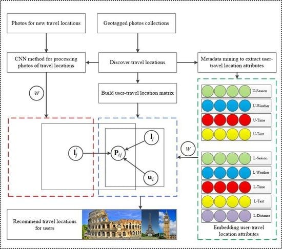
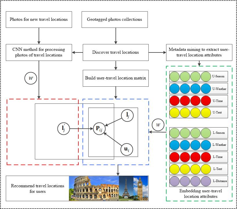
4. Methodology
4.1. Discovering Travel Locations from CCGPs
4.2. Obtaining Explicit Information
4.2.1. Contextual Information Modeling
- Time of day: weekday AM, weekday PM, weekend AM, and weekend PM.
- Season: spring (Mar-Apr-May), summer (Jun-Jul-Aug), autumn (Sept-Oct-Nov), and winter (Dec-Jan-Feb).
- Weather-temperature: hot (≥25 °C), warm (15–25 °C), cool (5–15 °C), and cold (<5 °C).
- Weather-sky condition: sunny, cloudy, rainy, snowy, and foggy.
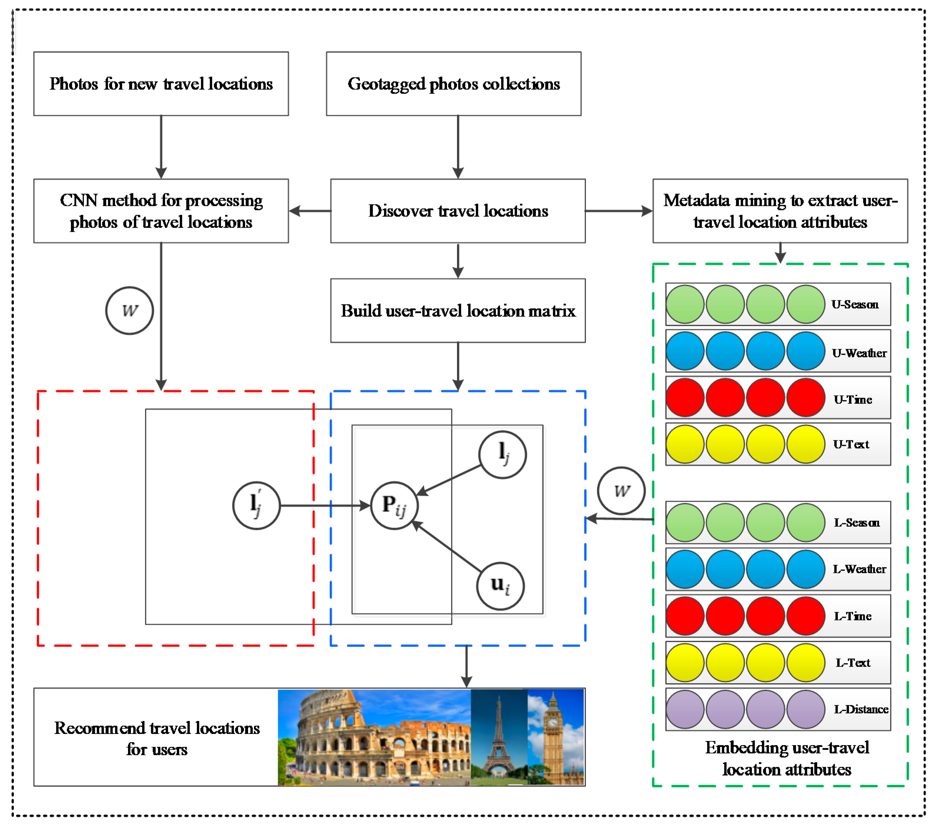
4.2.2. Textual Information Modeling
- Select parameters -𝐷𝑖r (), where is the topic distribution of document and 𝐷𝑖r () is the Dirichlet distribution of parameter 𝛼.
- For each word:
- Select a topic -multinomial ().
- Select a word -multinomial ().
4.3. Obtaining Explicit Information
4.4. Factorizing User–Travel Location Interaction
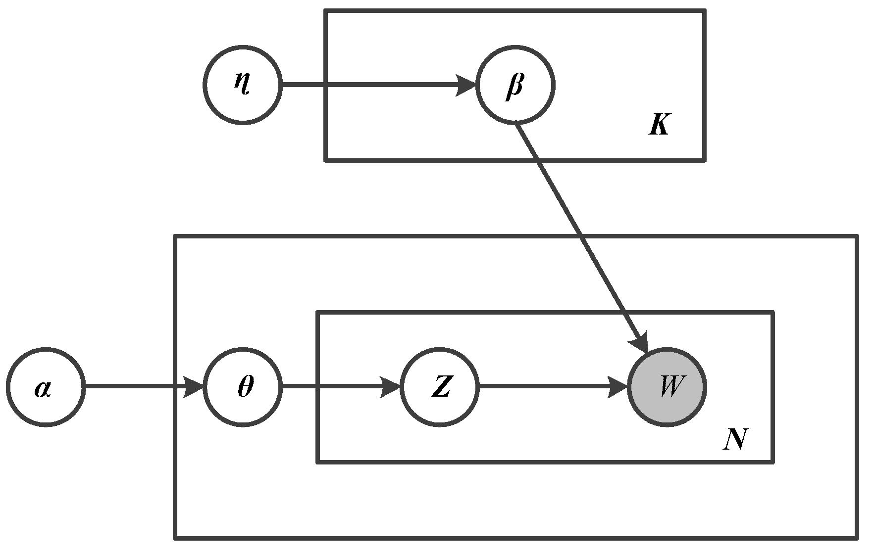
4.5. Exploiting Visual Content
4.6. Estimating Latent Factor from Photos
4.7. Travel Location Recommendation
4.8. The Learning Algorithm of CNNMF
| Algorithm 1. The proposed Framework CNNMF |
| Input: P, user–travel location preference matrix Simu(ui, uk): user–user similarities Siml(lj,lk):travel location–travel location similarities lj for lj ∈ Output: Latent factor vector of user and travel location ui, lj; 1: initialize the weight of VGG-16 on the place database 2: initialize ui, lj and 3: for each ui do 4: update by Equation (10) 5: end for 6: for each lj do 7: update by Equation (11) 8: end for 9: If travel location j is new then 10: estimate by CNN(W,fj) 11: update by Equation (12) 12: end if 13: return the top travel locations by Pij |
5. Experiments
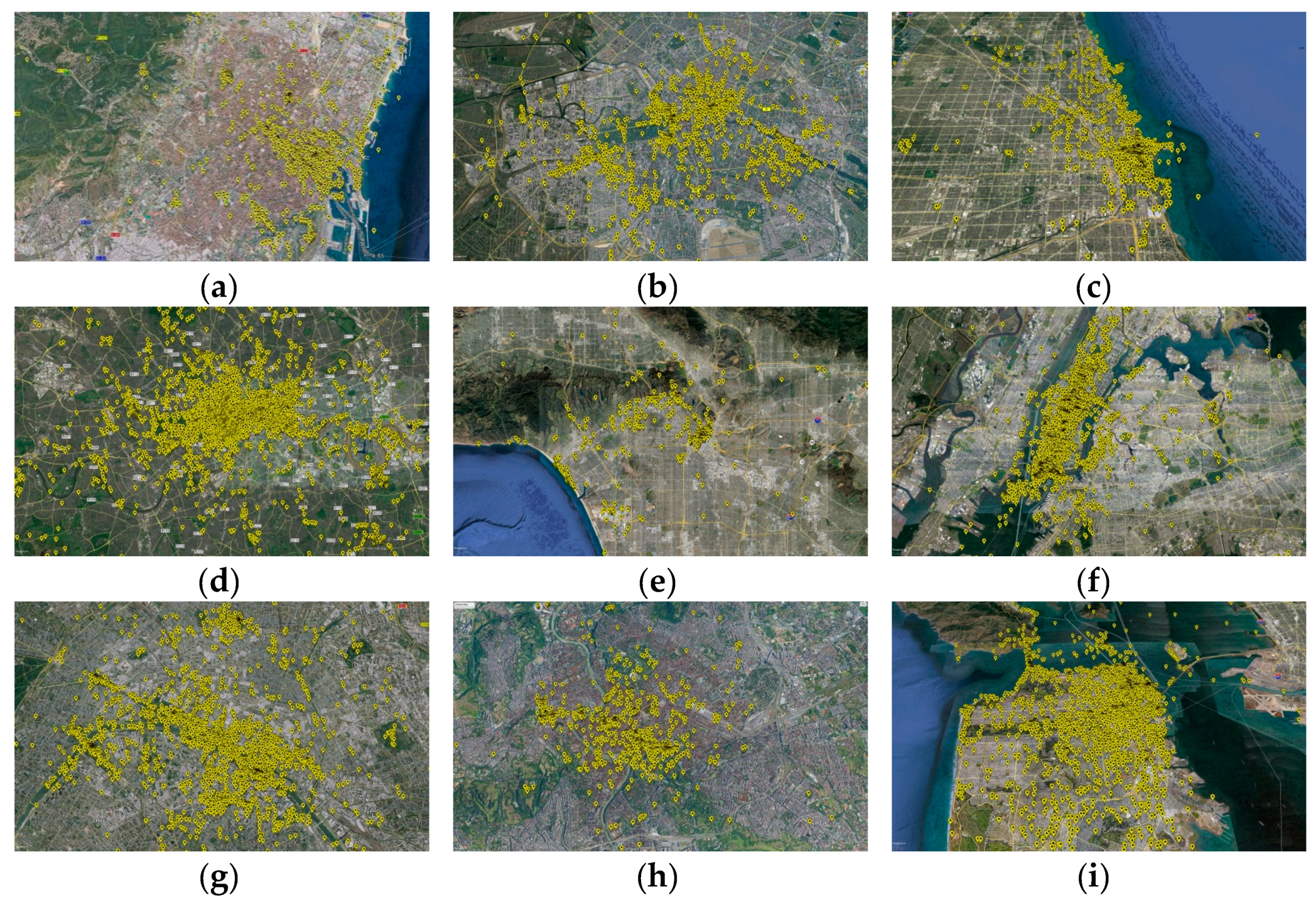
5.1. Dataset
5.2. Parameter Settings
- To enable P-DBSCAN to detect travel locations from CCGPs, we set a , radius m, and density ratio .
- To obtain the user–travel location interaction information, we empirically set a threshold of visit duration h.
- In all the following experiments based on matrix factorization methods, we set parameters , , , , and .
- CNN is employed to estimate the latent factors of new travel locations. The learning rate parameter is for epochs and mini-batch size is 128. The momentum is 0.9. The weight decay is 0.0005. The weights are randomly initialized following previous work [40].
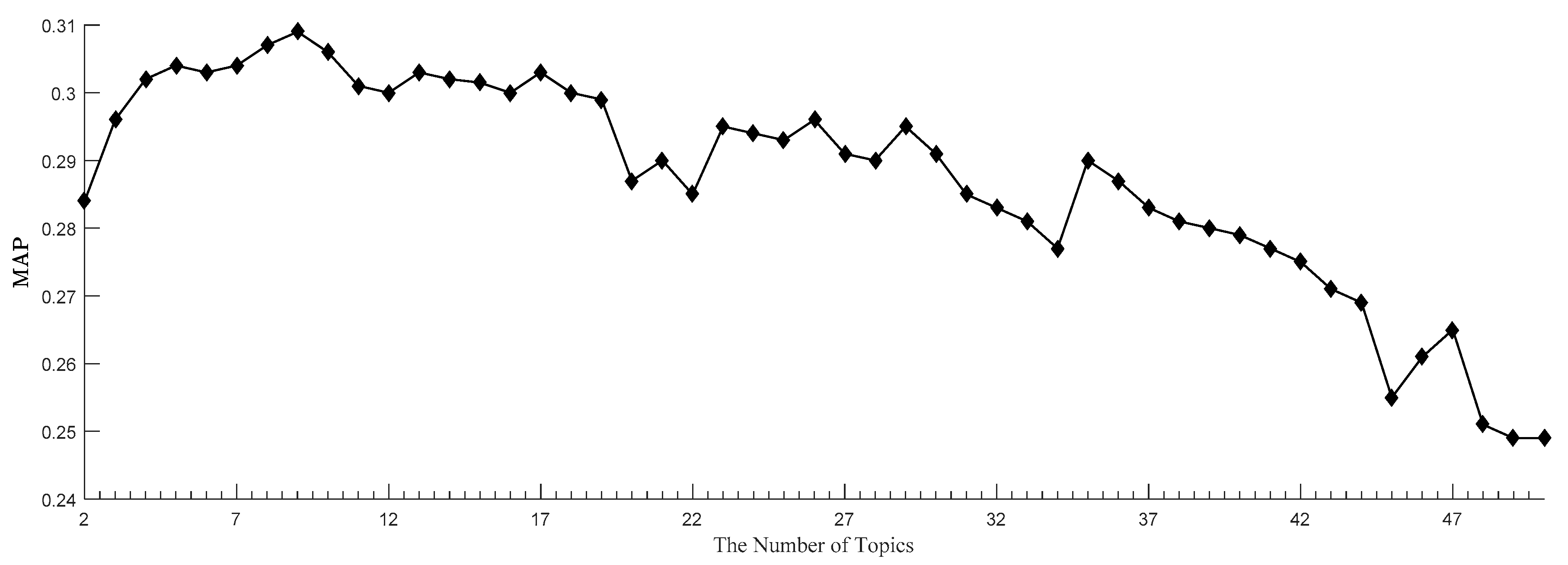
5.3. The Impact of Topic Number
5.4. The Impact of Diverse Types of Information
- Diverse types of information enhance recommendation performance to diverse degrees. According to influence degree, the information can be ranked as follows: season information > weather information > text information > time information > geographical distance information. The performance of eliminating “season” information is the lowest, which means that “season” information is the most important information to recommend travel location. The performance of eliminating “geographical distance” information is the highest, which means that “geographical distance” information is the most unimportant information, as most travel locations are not far from each other.
- The MAP of the proposed method is significantly better than those of the five other variants, which demonstrated that the proposed method integrates contextual, textual, and geographical information together and can thus provide improved recommendations.
5.5. The Performance Comparison of Recommendation Methods
- Dynamic topic model and matrix factorization (DTMMF): DTMMF integrates topic model with matrix factorization to recommend travel locations. DTM is used to obtain implicit information, while explicit information is obtained from past check-ins and visual contents (i.e., age and gender) to construct user and travel location profiles [9].
- Neural network-based Collaborative Filtering (NCF): NCF combines matrix factorization with multi-layer perceptron to capture nonlinear user–travel location interactions [41]. Visual content is not considered.
- Visual-enhanced probabilistic matrix factorization model (VPMF): VPMF uses visual features to learn user preferences by leveraging the past check-ins of users. Then, it integrates user preferences with travel location constraints for trip planning [42].
- Visual Bayesian personalized ranking (VBPR): VBPR extracts the visual features from photos using a pre-trained method without any context information [5]. The extracted visual feature is used to predict the scores of people’s opinions.
- Visual Content Enhanced POI recommendation (VPOI): VPOI uses joint learning of photo classification, matrix decomposition, and visual feature extraction tasks [29], to recommend travel locations to the user. The difference with the proposed method is that VPOI uses photos for joint learning of the latent factor vector representations.
- The proposed method beats other methods, i.e., DTMMF, NCF, VPMF, VBPR and VPOI, respectively, on average 35.21%, 32.65%, 31.22%, 22.87%, 9.5%.
- VPMF works better than DTMMF, which might be because VPMF extracts visual features directly from the whole photo, while DTMMF extracts only some attributes (i.e., age and gender) based on face recognition.
- VPOI works better than VBPR, which might be because VPOI models photos for both users and travel locations while VBPR only models photos for travel locations.
- The proposed method significantly outperforms VPOI. That is because of the incorporating of contextual (i.e., time, weather, and season), textual (i.e., tags), and geographical (i.e., distance) information, while VPOI only uses photos for joint learning of the latent factor vector representations.
- In general, the performance of all methods drops when we present the travel location cold start problem. For example, the performance of DTMMF decreases up to 14.65% in terms of MAP@10.
- The proposed method beats other methods, i.e., DTMMF, NCF, VPMF, VBPR and VPOI, respectively, on average 40.17%, 41.43, 40.17%, 29.06%, 11.63%, for cold start travel locations.
- The performance reduction of VBPR is much smaller than that of DTMMF, as VBPR learns an additional layer to exploit the visual dimensions, which can help to alleviate the travel location cold start problem, while DTMMF uses visual contents only to extract attributes (i.e., age and gender) based on face recognition.
- The proposed method of CNNMF significantly outperforms VPOI, while both methods use visual contents. The differences between the CNNMF and VPOI include: CNNMF directly obtains latent factor from its photos as descriptions of travel locations; while VPOI uses photos to help learn the latent factor vector representation.
6. Conclusions and Future Work
Author Contributions
Funding
Conflicts of Interest
References
- Majid, A.; Chen, L.; Chen, G.; Mirza, H.T.; Hussain, I.; Woodward, J. A context-aware personalized travel recommendation system based on geotagged social media data mining. Int. J. Geogr. Inf. Sci. 2013, 27, 662–684. [Google Scholar] [CrossRef]
- Liu, J.; Zhang, Z.; Liu, C.; Qiu, A.; Zhang, F. Exploiting two-dimensional geographical and synthetic social influences for location recommendation. ISPRS Int. J. Geo-Inf. 2020, 9, 285. [Google Scholar] [CrossRef]
- Sun, X.; Huang, Z.; Peng, X.; Chen, Y.; Liu, Y. Building a model-based personalised recommendation approach for tourist attractions from geotagged social media data. Int. J. Digit. Earth 2019, 12, 661–678. [Google Scholar] [CrossRef]
- Wang, Z.; Zhang, D.; Zhou, X.; Yang, D.; Yu, Z.; Yu, Z. Discovering and profiling overlapping communities in location-based social networks. IEEE Trans. Syst. Man Cybern. Syst. 2014, 44, 499–509. [Google Scholar] [CrossRef] [Green Version]
- Yang, D.; Zhang, D.; Yu, Z.; Wang, Z. A sentiment-enhanced personalized location recommendation system. In Proceedings of the 24th ACM conference on hypertext and social media, Paris, France, 1–3 May 2013; pp. 119–128. [Google Scholar]
- Zhang, J.D.; Chow, C.Y. iGSLR: Personalized geo-social location recommendation: A kernel density estimation approach. In Proceedings of the 21st ACM SIGSPATIAL International Conference on Advances in Geographic Information Systems, Orlando, FL, USA, 5–8 November 2013; pp. 334–343. [Google Scholar]
- Xu, Z.; Chen, L.; Chen, G. Topic based context-aware travel recommendation method exploiting geotagged photos. Neurocomputing 2015, 155, 99–107. [Google Scholar] [CrossRef]
- Shi, Y.; Serdyukov, P.; Hanjalic, A.; Larson, M. Nontrivial landmark recommendation using geotagged photos. ACM Trans. Intell. Syst. Technol. 2013, 4, 1–27. [Google Scholar] [CrossRef]
- Xu, Z.; Chen, L.; Dai, Y.; Chen, G. A dynamic topic model and matrix factorization-based travel recommendation method exploiting ubiquitous data. IEEE Trans. Multimed. 2017, 19, 1933–1945. [Google Scholar] [CrossRef]
- Kim, D.; Park, C.; Oh, J.; Lee, S.; Yu, H. Convolutional matrix factorization for document context-aware recommendation. In Proceedings of the 10th ACM Conference on Recommender Systems, Boston, MA, USA, 15–19 September 2016; pp. 233–240. [Google Scholar]
- Cai, G.; Lee, K.; Lee, I. Itinerary recommender system with semantic trajectory pattern mining from geo-tagged photos. Expert Syst. Appl. 2018, 94, 32–40. [Google Scholar] [CrossRef]
- Gao, H.; Tang, J.; Liu, H. gSCorr: Modeling geo-social correlations for new check-ins on location-based social networks. In Proceedings of the 21st ACM International Conference on Information and Knowledge Management, Maui, HI, USA, 29 October–2 November 2012; pp. 1582–1586. [Google Scholar]
- Gao, H.; Tang, J.; Liu, H. Addressing the cold-start problem in location recommendation using geo-social correlations. Data Min. Knowl. Discov. 2015, 29, 299–323. [Google Scholar] [CrossRef] [Green Version]
- Shi, H.; Chen, L.; Xu, Z.; Lyu, D. Personalized location recommendation using mobile phone usage information. Appl. Intell. 2019, 49, 3694–3707. [Google Scholar] [CrossRef]
- Van den Oord, A.; Dieleman, S.; Schrauwen, B. Deep content-based music recommendation. In Advances in Neural Information Processing Systems 26: 27th Annual Conference on Neural Information Processing Systems 2013, Lake Tahoe, NV, USA, 5–8 December 2013; NeurIPS: San Diego, CA, USA, 2013; pp. 2643–2651. [Google Scholar]
- Kim, Y. Convolutional neural networks for sentence classification. In Proceedings of the Conference on Empirical Methods in Natural Language Processing (EMNLP), Doha, Qatar, 25–29 October 2014; pp. 1746–1751. [Google Scholar]
- Yue-Hei Ng, J.; Yang, F.; Davis, L.S. Exploiting local features from deep networks for image retrieval. In Proceedings of the IEEE Conference on Computer Vision and Pattern Recognition Workshops, Boston, MA, USA, 7–12 June 2015; pp. 53–61. [Google Scholar]
- Jiang, S.; Qian, X.; Mei, T.; Fu, Y. Personalized travel sequence recommendation on multi-source big social media. IEEE Trans. Big Data 2016, 2, 43–56. [Google Scholar] [CrossRef]
- Liu, C.; Liu, J.; Xu, S.; Wang, J.; Liu, C.; Chen, T.; Jiang, T. A Spatiotemporal Dilated Convolutional Generative Network for Point-Of-Interest Recommendation. ISPRS Int. J. Geo-Inf. 2020, 9, 113. [Google Scholar] [CrossRef] [Green Version]
- Zheng, Y.T.; Zha, Z.J.; Chua, T.S. Mining travel patterns from geotagged photos. ACM Trans. Intell. Syst. Technol. 2012, 3, 1–18. [Google Scholar] [CrossRef]
- Chen, C.; Chen, X.; Wang, Z.; Wang, Y.; Zhang, D. ScenicPlanner: Planning scenic travel routes leveraging heterogeneous user-generated digital footprints. Front. Comput. Sci. 2017, 11, 61–74. [Google Scholar] [CrossRef]
- Majid, A.; Chen, L.; Mirza, H.T.; Hussain, I.; Chen, G. A system for mining interesting tourist locations and travel sequences from public geo-tagged photos. Data Knowl. Eng. 2015, 95, 66–86. [Google Scholar] [CrossRef]
- Cheng, A.J.; Chen, Y.Y.; Huang, Y.T.; Hsu, W.H.; Liao, H.Y.M. Personalized travel recommendation by mining people attributes from community-contributed photos. In Proceedings of the 19th ACM International Conference on Multimedia, Scottsdale, AZ, USA, 28 November–1 December 2011; pp. 83–92. [Google Scholar]
- Chen, Y.Y.; Cheng, A.J.; Hsu, W.H. Travel recommendation by mining people attributes and travel group types from community-contributed photos. IEEE Trans. Multimed. 2013, 15, 1283–1295. [Google Scholar] [CrossRef]
- Ke, X.; Zou, J.; Niu, Y. End-to-end automatic image annotation based on deep cnn and multi-label data augmentation. IEEE Trans. Multimed. 2019, 21, 2093–2106. [Google Scholar] [CrossRef]
- Kuang, H.; Zhu, S.; El Saddik, A. Boosting prediction of geo-location for web images through integrating multiple knowledge sources. In Proceedings of the 5th ACM on International Conference on Multimedia Retrieval, Shanghai, China, 23–26 June 2015; pp. 559–562. [Google Scholar]
- Xing, S.; Wang, Q.; Zhao, X.; Li, T. Content-aware point-of-interest recommendation based on convolutional neural network. Appl. Intell. 2019, 49, 858–871. [Google Scholar] [CrossRef]
- Weyand, T.; Kostrikov, I.; Philbin, J. Planet-photo geolocation with convolutional neural networks. In Proceedings of the 14th European Conference on Computer Vision—ECCV 2016, Amsterdam, The Netherlands, 11–14 October 2016; pp. 37–55. [Google Scholar]
- Wang, S.; Wang, Y.; Tang, J.; Shu, K.; Ranganath, S.; Liu, H. What your images reveal: Exploiting visual contents for point-of-interest recommendation. In Proceedings of the 26th International Conference on World Wide Web, Perth, WA, Australia, 3–7 April 2017; pp. 391–400. [Google Scholar]
- Crandall, D.J.; Backstrom, L.; Huttenlocher, D.; Kleinberg, J. Mapping the world’s photos. In Proceedings of the 18th International Conference on World Wide Web, Madrid, Spain, 20–24 April 2009; pp. 761–770. [Google Scholar]
- Yu, Y.; Zhao, Y.; Yu, G.; Wang, G. Mining coterie patterns from Instagram photo trajectories for recommending popular travel routes. Front. Comput. Sci. 2017, 11, 1007–1022. [Google Scholar] [CrossRef]
- Kisilevich, S.; Mansmann, F.; Keim, D. P-DBSCAN: A density based clustering algorithm for exploration and analysis of attractive areas using collections of geo-tagged photos. In Proceedings of the 1st International Conference and Exhibition on Computing for Geospatial Research & Application, Washington, DC, USA, 21–23 June 2010; pp. 1–4. [Google Scholar]
- Matsuo, S.; Shimoda, W.; Yanai, K. Twitter photo geo-localization using both textual and visual features. In Proceedings of the IEEE 3rd International Conference on Multimedia Big Data, Laguna Hills, CA, USA, 19–21 April 2017; pp. 22–25. [Google Scholar]
- Blei, D.M.; Ng, A.Y.; Jordan, M.I. Latent dirichlet allocation. J. Mach. Learn. Res. 2003, 3, 993–1022. [Google Scholar]
- Hu, Y.; Koren, Y.; Volinsky, C. Collaborative filtering for implicit feedback datasets. In Proceedings of the IEEE International Conference on Data Mining, Pisa, Italy, 15–19 December 2008; pp. 263–272. [Google Scholar]
- Simonyan, K.; Zisserman, A. Very deep convolutional networks for large-scale image recognition. In Proceedings of the International Conference on Learning Representations 2015, San Diego, CA, USA, 7–9 May 2015; pp. 1409–1556. [Google Scholar]
- Donahue, J.; Jia, Y.; Vinyals, O.; Hoffman, J.; Zhang, N.; Tzeng, E.; Darrell, T. Decaf: A deep convolutional activation feature for generic visual recognition. In Proceedings of the 31th Conference on Machine Learning, Beijing, China, 21–26 June 2014; pp. 647–655. [Google Scholar]
- Sharif Razavian, A.; Azizpour, H.; Sullivan, J.; Carlsson, S. CNN features off-the-shelf: An astounding baseline for recognition. In Proceedings of the 27th IEEE Conference on Computer Vision and Pattern Recognition Workshops, Columbus, OH, USA, 24–27 June 2014; pp. 806–813. [Google Scholar]
- He, K.; Sun, J. Convolutional neural networks at constrained time cost. In Proceedings of the IEEE Conference on Computer Vision and Pattern Recognition, Boston, MA, USA, 7–12 June 2015; pp. 5353–5360. [Google Scholar]
- Zhou, B.; Lapedriza, A.; Xiao, J.; Torralba, A.; Oliva, A. Learning deep features for scene recognition using places database. In Proceedings of the Advances in Neural Information Processing Systems 27: Annual Conference on Neural Information Processing Systems 2014, Montreal, QC, Canada, 8–13 December 2014; pp. 487–495. [Google Scholar]
- He, R.; McAuley, J. VBPR: Visual bayesian personalized ranking from implicit feedback. In Proceedings of the 30th AAAI Conference on Artificial Intelligence, Phoenix, AZ, USA, 12–17 February 2016. [Google Scholar]
- Zhao, P.; Xu, C.; Liu, Y.; Sheng, V.S.; Zheng, K.; Xiong, H.; Zhou, X. Photo2trip: Exploiting visual contents in geo-tagged photos for personalized tour recommendation. In Proceedings of the the 25th ACM international conference on Multimedia, Silicon Valley, CA, USA, 23–27 October 2017. [Google Scholar]


| Photo ID | User ID | Tags | Date Taken | Latitude | Longitude |
|---|---|---|---|---|---|
| pic00139703 | user0001435 | France, Paris, honeymoon, Eiffel tower | 2006-03-26 01:33:10 | 48.873747 | 2.324981 |
| pic00054003 | user000908 | England, London, Thames, Tower bridge | 2006-05-05 18:05:55 | 51.50942 | 0.107266 |
| Cities | Users | Travel Locations | Check-in | Photos | |
|---|---|---|---|---|---|
| (Filtered) | (Row) | ||||
| Barcelona | 122 | 37 | 289 | 5853 | 15,704 |
| Berlin | 100 | 36 | 273 | 11,083 | 13,420 |
| Chicago | 134 | 64 | 416 | 12,304 | 22,104 |
| London | 270 | 82 | 1468 | 14,256 | 43,557 |
| Los Angeles | 101 | 30 | 65 | 3961 | 10,122 |
| New York | 228 | 71 | 782 | 12,049 | 34,374 |
| Paris | 273 | 67 | 1120 | 10,879 | 24,507 |
| Rome | 125 | 30 | 309 | 7828 | 18,416 |
| San Francisco | 175 | 56 | 842 | 10,060 | 24,572 |
| Total | 1528 | 473 | 5564 | 88,273 | 206,776 |
| Performance | Text (txt) | Distance (dis) | Season (s) | Weather (w) | Time (t) | CNNMF |
|---|---|---|---|---|---|---|
| MAP@1 | 0.456 ± 0.043 | 0.632 ± 0.051 | 0.397 ± 0.045 | 0.446 ± 0.082 | 0.492 ± 0.072 | 0.653 ± 0.012 |
| MAP@5 | 0.320 ± 0.054 | 0.364 ± 0.066 | 0.281 ± 0.062 | 0.313 ± 0.082 | 0.322 ± 0.085 | 0.404 ± 0.013 |
| MAP@10 | 0.215 ± 0.044 | 0.242 ± 0.072 | 0.191 ± 0.071 | 0.213 ± 0.063 | 0.219 ± 0.077 | 0.271 ± 0.022 |
| MAP@20 | 0.136 ± 0.031 | 0.152 ± 0.043 | 0.122 ± 0.082 | 0.135 ± 0.065 | 0.139 ± 0.046 | 0.171 ± 0.011 |
| Performance | (a) | (b) | (c) | (d) | (e) | (f) | Improv. |
|---|---|---|---|---|---|---|---|
| DTMMF | NCF | VPMF | VBPR | VPOI | CNNMF | f vs. best | |
| MAP@1 | 0.475 ± 0.061 | 0.492 ± 0.071 | 0.512 ± 0.061 | 0.584 ± 0.029 | 0.623 ± 0.097 | 0.662 ± 0.018 | 6.26% |
| MAP@5 | 0.358 ± 0.081 | 0.359 ± 0.039 | 0.351 ± 0.081 | 0.367 ± 0.074 | 0.391 ± 0.075 | 0.415 ± 0.012 | 6.19% |
| MAP@10 | 0.198 ± 0.072 | 0.200 ± 0.073 | 0.201 ± 0.072 | 0.203 ± 0.077 | 0.231 ± 0.070 | 0.271 ± 0.022 | 17.32% |
| MAP@20 | 0.115 ± 0.025 | 0.118 ± 0.085 | 0.120 ± 0.025 | 0.130 ± 0.098 | 0.158 ± 0.041 | 0.171 ± 0.013 | 8.23% |
| Performance | (a) | (b) | (c) | (d) | (e) | (f) | Improv. |
|---|---|---|---|---|---|---|---|
| DTMMF | NCF | VPMF | VBPR | VPOI | CNNMF | f vs. best | |
| MAP@1 | 0.421 (11.37%) | 0.441 (11.56%) | 0.454 (11.33%) | 0.532 (8.90%) | 0.585 (6.10%) | 0.623 (5.89%) | 6.50% |
| MAP@5 | 0.315 (12.01%) | 0.318 (11.42%) | 0.320 (8.83%) | 0.331 (9.81%) | 0.362 (7.42%) | 0.395 (4.82%) | 9.12% |
| MAP@10 | 0.169 (14.65%) | 0.173 (13.5%) | 0.175 (12.94%) | 0.182 (10.34%) | 0.214 (7.36%) | 0.255 (5.90%) | 19.16% |
| MAP@20 | 0.101 (12.17%) | 0.106 (10.17%) | 0.105 (12.50%) | 0.116 (10.77%) | 0.145 (8.23%) | 0.162 (5.26%) | 11.73% |
© 2020 by the authors. Licensee MDPI, Basel, Switzerland. This article is an open access article distributed under the terms and conditions of the Creative Commons Attribution (CC BY) license (http://creativecommons.org/licenses/by/4.0/).
Share and Cite
Ameen, T.; Chen, L.; Xu, Z.; Lyu, D.; Shi, H. A Convolutional Neural Network and Matrix Factorization-Based Travel Location Recommendation Method Using Community-Contributed Geotagged Photos. ISPRS Int. J. Geo-Inf. 2020, 9, 464. https://0-doi-org.brum.beds.ac.uk/10.3390/ijgi9080464
Ameen T, Chen L, Xu Z, Lyu D, Shi H. A Convolutional Neural Network and Matrix Factorization-Based Travel Location Recommendation Method Using Community-Contributed Geotagged Photos. ISPRS International Journal of Geo-Information. 2020; 9(8):464. https://0-doi-org.brum.beds.ac.uk/10.3390/ijgi9080464
Chicago/Turabian StyleAmeen, Thaair, Ling Chen, Zhenxing Xu, Dandan Lyu, and Hongyu Shi. 2020. "A Convolutional Neural Network and Matrix Factorization-Based Travel Location Recommendation Method Using Community-Contributed Geotagged Photos" ISPRS International Journal of Geo-Information 9, no. 8: 464. https://0-doi-org.brum.beds.ac.uk/10.3390/ijgi9080464