Spatial Mismatch between the Supply and Demand of Urban Leisure Services with Multisource Open Data

Abstract

Understanding the balance between the supply and demand of leisure services (LSs) in urban areas can benefit urban spatial planning and improve the quality of life of residents. In cities in developing countries, the pursuit of rapid economic growth has ignored residents’ demand for LSs, thereby leading to a high demand for and short supply of these services. However, due to the lack of relevant research data, few studies have focused on the spatial mismatch in the supply and demand of LSs in urban areas. As typical representatives of multisource geographic data, social sensing data are readily available at various temporal and spatial scales, thus making social sensing data ideal for quantitative urban research. The objectives of this study are to use openly accessible datasets to explore the spatial pattern of the supply and demand of LSs in urban areas and then to depict the relationship between the supply and demand by using correlation analysis. Therefore, taking Beijing, China, as an example, the LS supply index (SI) and societal needs index (SNI) are proposed based on open data to reflect the supply and demand of LSs. The results show that the spatial distribution of the LS supply and demand in Beijing varies with a concentric pattern from the urban center to suburban areas. There is a strong correlation between the supply and demand of commercial and multifunctional services in Chaoyang, Fengtai, Haidian and Shijingshan, but there is no obvious correlation between the supply and demand of ecological and cultural services in Beijing. Especially in Dongcheng and Xicheng, there is no obvious correlation between the supply and demand of all services. The proposed approach provides an effective urban LS supply and demand evaluation method. In addition, the research results can provide a reference for the construction of “happy cities” in China.

1. Introduction

Urbanization, as a global phenomenon, has one of the most irreversible impacts on the global biosphere [1,2]. In its report “Prospects for World Urbanization in 2014”, the United Nations Department of Economic and Social Affairs, P. D (2014) predicted that with the acceleration of urbanization, by 2050, more than 70% of the global population will live in cities. As the world’s most-populated country, China has made remarkable achievements in urban construction and economic development [3]. However, one of the main consequences of the population explosion and economic prosperity is the serious conflict between the increased demand and lack of resources in urban areas. In addition, this very same phenomenon also brings more inequality worldwide, with some areas benefiting more from public investments and economic growth than others [4,5].

Representing one of the four basic functions of the city (dwelling, work, transportation, and leisure) [6,7], leisure is one of the most frequently considered activities in the planning process [8], and locations are needed to provide local residents with leisure, entertainment and other services [9]. Urban planning and human activity may affect the provision and delivery process of urban leisure services (LSs). For example, urban planning affects the provision of LSs by determining the location and biophysical features of leisure spaces [10,11]. LSs have been classified in a variety of ways; most commonly, LSs are divided into four categories: ecological leisure (EL), business leisure (BL), cultural leisure (CL) and multifunctional leisure (ML). Studies [12,13] found that leisure can enhance the happiness of urban residents more than income, health, or social relations, mainly because cities with more leisure are more suitable for family life and entertainment; therefore, leisure attracts many people, especially those with high-level talents, thereby further increasing the city’s attraction and the happiness of its residents [14]. Carlino also noted that residents with high education levels prefer cities that provide attractive leisure [15]. Thus, leisure has become an important factor for people in choosing where to live. If a city does not consider the configuration of leisure while developing, residents’ attitudes toward the government will be pessimistic.

Unfortunately, most governments have focused on the construction of “smart cities”, but “happy cities” is an advanced version of the “smart cities” concept. Compared with the design of a traditional smart city, which focuses on the technical level—that is, basic networks, sensing equipment, cloud computing facilities, and basic information resources—the construction of a happy city places more emphasis on the interaction between “technology” and “people”; notably, the actual needs of “people” are considered the top-level design objective, and improving the happiness and satisfaction of “people” is the core of the conceptual framework. For decades, the measures of happiness have been the gross domestic product (GDP) and human development index (HDI). However, there has been a growing criticism of depending on the standard of living as the only measure of happiness because the standard of living does not adequately portray well-being [16]. Leisure can contribute to subjective well-being (SWB) [17]. Clearly, involvement in daily leisure experiences (more than the GDP or HDI) increases the amount of direct pleasure that is perceived from participating in routine activities [17]. Urban residents should have equal opportunities to enjoy the benefits of urban LSs. Thus, the equity of urban LSs is a priority in constructing a happy city and a sign of civilization and progress in modern society [18,19]. It is thus necessary to develop a better understanding of the distribution of and the relationship between LS supply and demand to inform urbanists and city planners.

The remainder of this paper is organized as follows: Section 2 reviews related work. Section 3 introduces the materials and methods. Section 4 presents a case study to explore the spatial mismatch and spatial distribution of LSs in Beijing, China. Section 5 discusses the result and limitations. Section 6 concludes with a brief summary of this paper.

2. Related Work

“Supply and demand mismatch” refers to the mismatch of service supply and human demand within the defined spatial scope. For a long time, the lack of urban spatial temporal information was a major obstacle in studying and solving urban problems. In recent years, the development of remote sensing technology and computer technology has led to the creation of new data sources for urban research. A growing number of planners and researchers have realized the importance of urban public service facilities for urban residents. However, only a few have paid attention to the supply and demand pattern of urban multiple LSs, and most of them only paid attention to the green space that can provide ecological leisure services and ignored the commercial, cultural and multifunctional leisure services. Therefore, in the literature review, we mainly focus on and draw on the research of urban ecological leisure services.

According to the research method used, the current research can be divided into three categories: (1) index construction methods, (2) analysis methods, and (3) mixed methods. Index construction methods measure the degree of supply-demand matching according to the ratio of the service facility scale to the population within a certain range. For example, Karsten Grunewald [20] constructed an index system that included the green area, green area to population ratio, commuting distance, etc., to reveal the degree of matching between the supply and demand of daily LSs in urban green spaces in Germany. Fan [21] constructed a comprehensive index based on the quality and accessibility of green spaces and evaluated the supply pattern and evolution characteristics of recreational services at two scales (100 m grid units and municipal district) in Shanghai; Chen [22] used the ecosystem services supply and demand ratio (ESDR) to express the relationship between the ecosystem service (ES) supply and demand and to calculate the ES supply and demand in Wuhan, China. Analysis methods based on geographic information systems (GISs) commonly use GIS tools, such as network analysis, buffer analysis and spatial overlay analysis, to analyze supply and demand matching. For example, Gupta K. [23] used buffer zone analysis and network analysis to reveal the supply–demand matching degree of the Delhi green space in India; Maria Susana Orta Ortiz [9], using recreation and the food supply as an example, developed a methodology based on a quantitative explicit comparison and GIS network analysis to assess the unsatisfactory demand in Havana, Cuba. Mixed methods are suitable for simultaneously analyzing different data formats (qualitative and quantitative). For example, Kati Vierikko [24] used interview data and statistical data to analyze the direct relationship between the supply and demand of entertainment related to urban lake ecosystems in Finland by using a comprehensive ecosystem service method. Burkhard et al. [25] presented an easy-to-apply concept based on a matrix linking spatial explicit biophysical landscape units to ecological integrity and ecosystem service supply and demand.

Although the above methods have contributed to the detection of a mismatch between the supply and demand of urban LSs, the following problems generally exist:

(1) The questionnaires or statistical data used in most studies have low temporal and spatial resolutions and, therefore, may not meet the decision-making requirements.

(2) Currently, there is no systematic and comprehensive research on the supply and demand of urban LSs. Most current studies considered LSs as being part of urban ESs [3,9,20], and thus covered only green spaces and parks that may provide outdoor LSs while ignoring services such as culture leisure and entertainment leisure.

(3) Most studies on urban LSs often did not properly consider access to leisure spaces; e.g., these studies did not consider transportation infrastructures [26].

To address these issues, we employ openly accessible datasets (such as point-of-interest (POI) data, population data and GDP data) instead of census and questionnaire data to evaluate and analyze urban LSs. POI data, which are obtained from web maps, are point data on real geographical entities. POI data have location-rich semantic information [27], high precision, wide coverage, and rapid updates and are widely applied to understand urban environments [28,29]. Moreover, some POI categories, such as stadiums and parks, are closely related to human leisure, while other categories of POIs, such as companies, have a weak supply of leisure and even have an exclusion effect. In addition, population density data reflect the intensity of human activities, while GDP data reflect the intensity of socioeconomic distribution. Combining the advantages of these data boasts considerable potential for achieving better insights into urban LS supply and demand patterns. To the best of our knowledge, at a large spatial scale and a high level of detail, a gap remains in the research on spatial mismatch for urban LS supply and demand. In this context, this paper explores the spatial mismatch between the urban LS supply and societal needs by using multisource data. The specific objectives of the study are (a) to identify the areas of LS supply-demand mismatch, (b) to analyze the relationship between the supply and demand of urban LSs, and (c) to provide reference for urban construction.

3. Materials and Methods

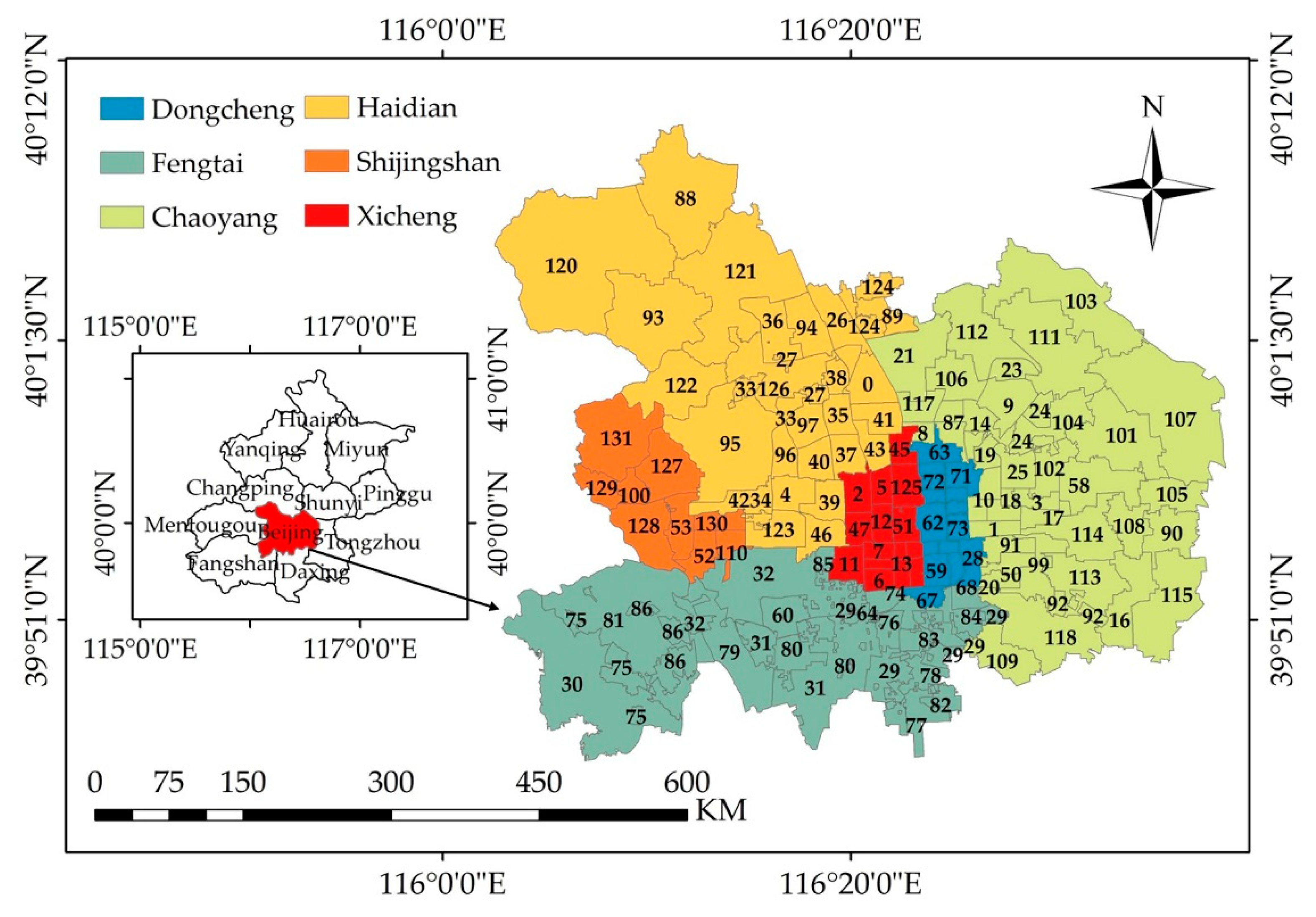
3.1. Study Area

Beijing has a population of approximately 21.54 million people living within an area of approximately 16,410.54 km². Additionally, Beijing is the capital of the People’s Republic of China and is the political center, cultural center, international exchange center, and scientific and technological innovation center of China. A UN report noted that the HDI of Beijing ranks second among those of the cities in China. In 2019, Beijing’s GDP was 3537.13 billion yuan, and the total retail sales of consumer goods was 1227.01 billion yuan. However, unfortunately, Beijing was not named as having been in the top 30 of China’s happiest cities in 2019. The rapid economic growth in Beijing has led to an imbalanced and mismatched spatial distribution of public facilities and services.

To accelerate the development of urban LSs in Beijing, the government has proposed plans and measures to enhance the construction of urban leisure spaces. For example, the Beijing urban master plan (2016–2035), which was adopted in 2017, identified the sustainable development of urban areas as the main goal of urban planning. Achieving this goal requires, among other things, increasing the construction of recreational areas, green spaces and sports leisure spaces to preserve and enhance the benefits of urban leisure spaces, thereby contributing to citizens’ well-being and quality of life. The “Measures to Further Improve the Economy and Promote Consumption Growth in Beijing” was proposed to establish a number of functional nighttime landmarks, nighttime business districts, and nighttime living areas in Beijing by the end of 2021. Additionally, the “Beijing Shijingshan Capital Culture Recreation and Leisure District (CRD) Construction Action Plan” was proposed to build numerous leisure facilities and public green spaces and transform old buildings into museums, art centers and galleries to create an attractive leisure environment. Since 2008, these plans have profoundly affected Beijing’s land use and urban development. Thus, government departments need to quickly and effectively obtain data on the area and location of each urban leisure space. This urban planning requirement is one of the motivations of this study. Therefore, we selected six central areas (Dongcheng, Xicheng, Chaoyang, Fengtai, Shijingshan, and Haidian) in Beijing as the study area to evaluate the distribution of the supply and demand of LSs (Figure 1).

3.2. Data Sources and Preprocessing

In this study, six types of data were used. The administrative boundary in Beijing is the basic dataset. Urban LS POIs and traffic hub data were used to calculate the LS supply index (SI), and urban residential POIs, population data and GDP data were used to calculate societal needs index (SNI) values. The specific sources of the above data, their spatiotemporal resolutions and the preprocessing steps are described below.

3.2.1. POI Data

The POI data used in this study were collected in 2019 from the most popular online map service provider in China: Gaode Map (https://www.amap.com/). We compiled a crawler program and collected the POI data by using the free interface provided by the Gaode application programming interface (API) (https://lbs.amap.com/api/ios-sdk/guide/map-data/poi/). A total of 1,285,920 POIs in Beijing were obtained. Among the Gaode POIs, there were 23 first-level, 264 second-level and 869 third-level classifications; we selected 7 first-level (food and beverages, shopping, sports and recreation, tourist attraction, daily life service, science/culture and education service and place name and address), 24 second-level and 87 third-level classifications related to LSs for reclassification. Based on previous research [6], LSs were reclassified into 4 types: EL, BL, CL, and ML. The reclassified detailed information is shown in

Table 1. Reclassification of leisure services.

ID	Leisure Service Category	Corresponding POI Categories in the Baidu Map (Second-Level)	Corresponding POI Categories in the Baidu Map (Third-Level)
1	Ecological leisure (EL)	Natural place name, scenery spot	National view spot, provincial view spot, beach
		park and square	Zoo, park, botanical garden, aquarium
2	Business leisure (BL)	Theatre and cinema, recreation center, commercial Street, coffee house, tea house, ice-cream shop, dessert house, bath and massage center	All
3	Cultural leisure (CL)	Arts organization, cultural palace, planetarium, science and technology museum, library, art gallery, convention and exhibition center, exhibition hall, museum, tourist attraction related	All
		scenery spot	World heritage, memorial hall, Buddhist and Taoist temple, church, scenery spot, mosque
4	Multifunctional leisure (ML)	Sports stadium, golf related, recreation place	All
		park and square	Park and square, city plaza, facilities within the park

. A total of 16,112 traffic hubs (subway stations and bus stations) and 52,736 residential POIs (accommodation service and commercial houses) were included in the study area.

3.2.2. Nighttime Light (NTL) Data

The NTL data (annual synthetic data in 2015 and monthly synthetic data in 2019) were obtained from the National Centers for Environment Information (https://www.ngdc.noaa.gov/eog/viirs/download_dnb_composites.html). The unit is nanowatts/cm²/sr. We used the invariant region model that was proposed by Wu [30] to correct the outliers in the data. Since the Suomi National Polar-orbiting Partnership Visible Infrared Imaging Radiometer Suite (NPP/VIIRS) (NTL image) data in 2019 are monthly synthetic data, they were averaged to obtain annual images [31]. The spatial resolution was 500 m.

3.2.3. Population and GDP Data

The population and GDP data from 2015 were obtained from the Resource and Environment Data Cloud Platform (http://www.resdc.cn/) in raster format. Each cell value of the 1-km grid of the spatial distribution of population data represents the population within the cell range (1 km²) in units of person/km². Additionally, each cell value of the 1-km grid of the spatial distribution of the GDP represents the total GDP within the cell range (1 km²) in units of ten thousand yuan/km². The original projection of the GDP and population data is the Albers Equal Area Conic projection. Additionally, we resampled 500-m data to obtain 1-km data.

NTL data are used to characterize the intensity and distribution of human activities [32,33], the population density [33,34] and economic vitality [35,36] due to the strong linear correlations between NTL data and these factors. In addition, Liu [37] and Li [35] found that there is a strong correlation between NTL and population and GDP data and developed a linear model. Therefore, to approximate the population density and economic data for 2019, we developed spatial relationship models for NTL-population data and NTL-GDP data.

$$y_{2019}=Int(\frac{y_{2015\times (x_{2019}+esp)}}{x_{2015}+esp})$$

(1)

where $y_{2019}$ is the population or GDP in 2019; $y_{2015}$ is the population or GDP in 2015; $x_{2015}$ and $x_{2019}$ are the NTL data in 2015 and 2019, respectively; $esp$ is a very small number, and its role is to prevent the population density from being invalid when the nighttime light value is 0; and $Int$ means to take an integer.

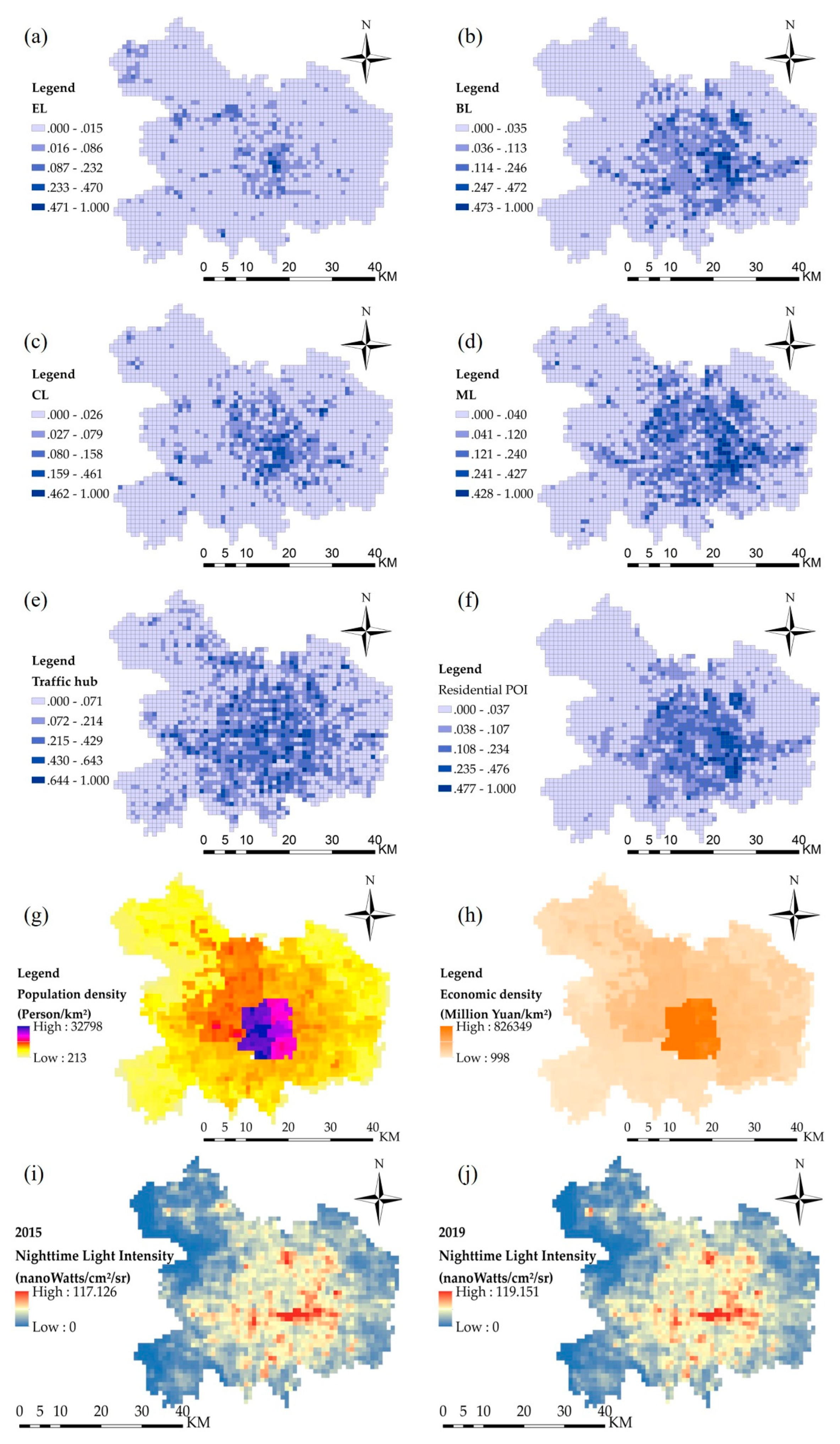
According to the above method, the population and GDP of the 1-km grids in 2019 were obtained. In addition, by using projections and transformations tools in ArcGIS, all of the data were transformed into a uniform projection (Alerts) at a resolution of 1 km. These data were extracted for the Beijing urban area by using the administrative boundary as a mask polygon (Figure 2).

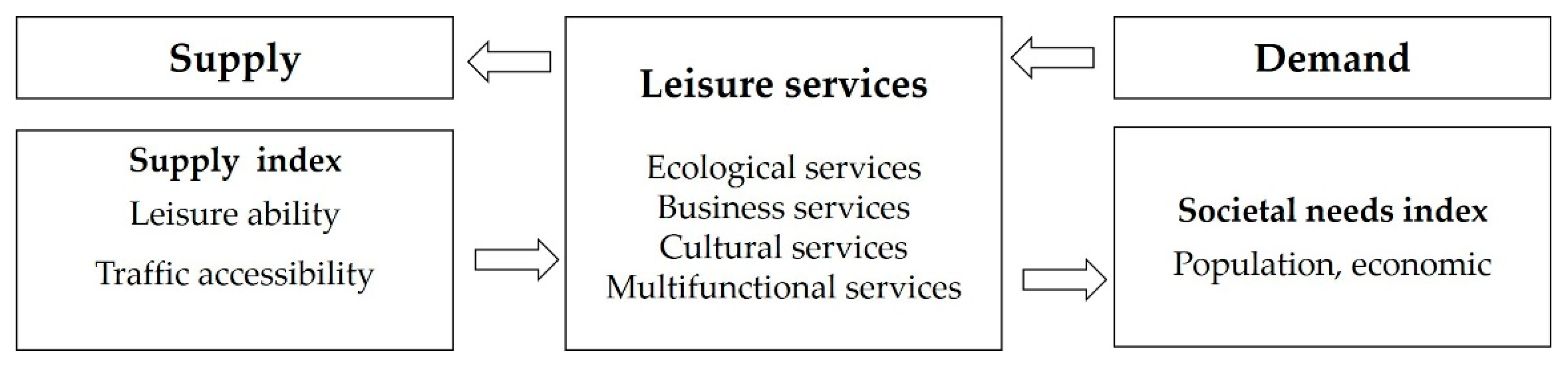
3.3. Calculation of LS Supply and Demand Index

Figure 3 illustrates the conceptual framework upon which the LS supply–demand assessments have been developed.

3.3.1. Supply Index of LSs

The distribution of LSs in the study area and the LS per unit area in different research units were calculated and analyzed by quantifying different types of LSs. The proportion of LSs was calculated based on the number of LS POIs relative to the total number of POIs; the proportion of LSs reflects the supply intensity of LSs. In addition, studies [26,38,39] have shown that leisure is associated with the ability of people to access leisure areas. Thus, leisure areas are inaccessible to society due to the lack of road or path networks. The greater the density of traffic hubs in a region is, the stronger the accessibility of the region; accessibility is the basic characterization of the ability of a region to provide LSs. Additionally, correlation analysis results show that there is no strong correlation between the ratio of LS POIs and the ratio of traffic hubs (the correlation coefficient is 0.376).

$$S{I}_i=L_i\times T_i$$

(2)

where $S{I}_i$ is the SI of LSs in area $i$, $L_i$ is the ratio of LS POIs in area $i$ to the total number of LS POIs, and $T_i$ is the ratio of the traffic hub in area $i$ to the total number of traffic hubs in the study area.

3.3.2. Societal Needs Index of LSs

In this study, the demand for urban LSs was interpreted based on human consumption capacity and activity intensity. Based on literature analysis [9,38,40] and the availability and temporal range of the data, two typical indicators were selected; namely, the population density and economic density, to reflect the demand for LSs in the region [40,41]. The population density directly reflects the degree of human demand for LSs in an area. Current studies [40] use GDP information to quantitatively estimate the willingness of residents to pay and characterize their economic ability. In general, the higher the GDP in a region is, the better the economic ability of the residents in the region, and the stronger the ability to purchase LSs [42,43].

Based on a correlation analysis of raster data, there was no obvious correlation between population and economic level and the ratio of residential POIs (correlation coefficients are 0.174, 0.352 and 0.349). Therefore, we proposed a comprehensive index model to measure the human demand for LSs.

$$SN{I}_i=R_i\times P_i\times E_i$$

(3)

where $SN{I}_i$ is the index of the demand for LSs in area $i$, $R_i$ is the ratio of residential POIs in area $i$ to the total number of residential POIs, and $P_i$ and $E_i$ represent the ratio of population and economic level in area $i$ to the total population size and economic level, respectively. All dependent variables were preprocessed using the min-max normalization method before modeling.

3.3.3. Analysis of the Supply-Demand Pattern of LSs

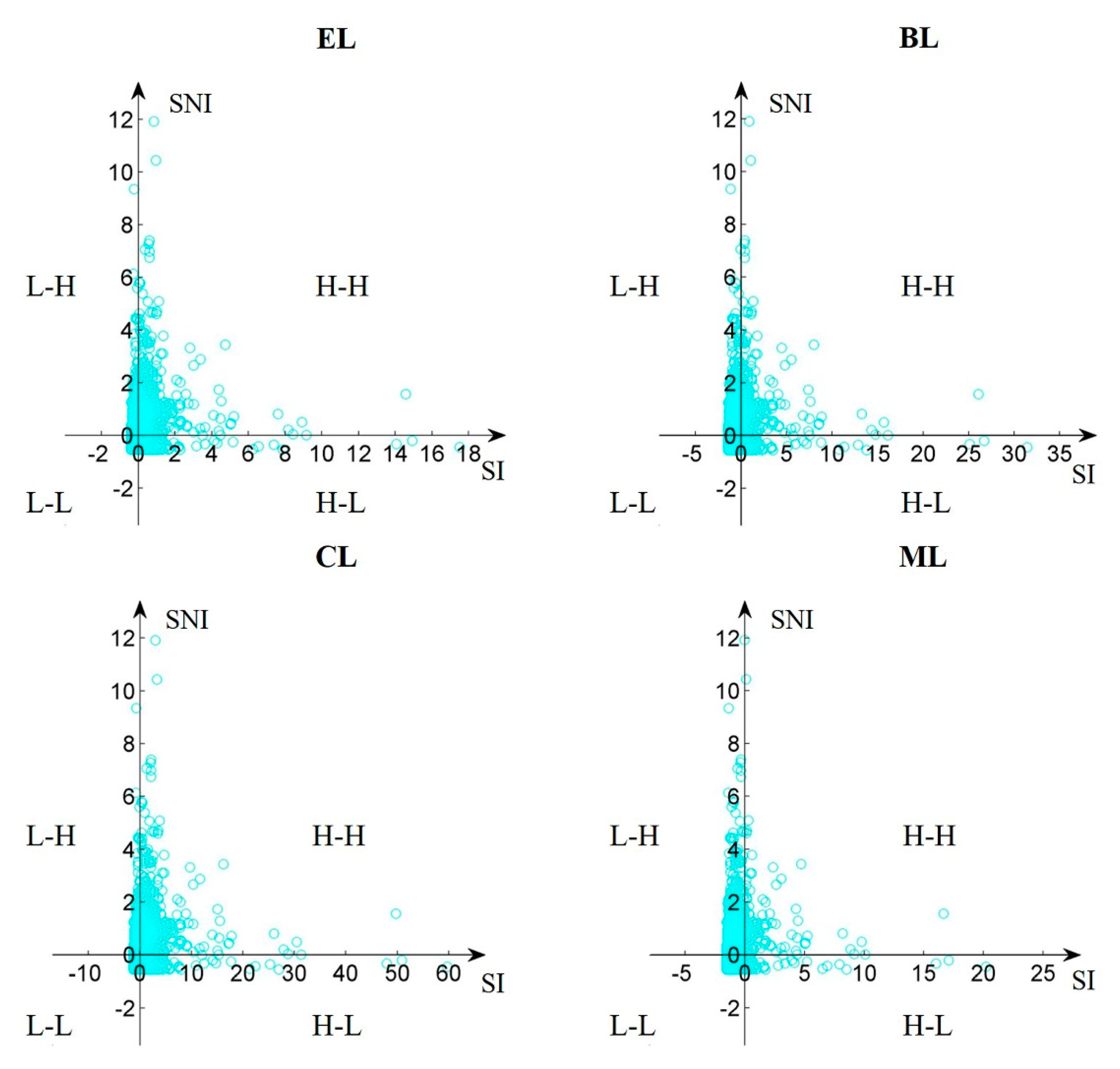
Since SI and SNI have different dimensions and orders of magnitude, the data needed to be standardized before calculating the supply and demand pattern. Z-score standardization was used to standardize SI and SNI. Additionally, the standardized SI was plotted on the x-axis, and the standardized SNI was plotted on the y-axis; thus, four quadrants were generated: High supply-High demand (H-H), Low supply-High demand (L-H), Low supply-Low demand (L-L) and High supply-Low demand (H-L). The specific formula is as follows:

$$x^{*}=\frac{x_i-\overline{x}}{\sigma }$$

(4)

$$\overline{x}=\frac{1}{n}{\displaystyle \sum }_{i=1}^n{x}_i$$

(5)

$$\sigma =\sqrt{\frac{1}{n}{\displaystyle \sum }_{i=1}^n{\left(x_i-\overline{x}\right)}^2}$$

(6)

where $x^{*}$ is the standardized SI or SNI; $n$ is the total number of regions; and $\overline{x}$ and $\sigma$ indicate the average and standard deviation, respectively, of SI or SNI in all regions in urban areas. The spatial distribution of standardized indices SI or SNI were overlaid in ArcGIS 10.2 to analyze the mismatching pattern.

3.4. Analysis of the Relationship between the LS Supply and Demand

In this study, the SI and SNI were used to analyze the relationship between LS supply and demand. We use the commonly used Spearman correlation coefficient [44] to assess the relationship between the supply and demand of LS. The purpose of correlation analysis is to determine the degree of influence of one variable on another by analyzing the interactions between variables, and the results of correlation analysis are expressed by the correlation coefficient and significance degree [45,46].

Due to the differences in socioeconomic level and population distribution in different regions in Beijing, China, Beijing was divided into 6 zones: Dongcheng, Xicheng, Chaoyang, Fengtai, Shijingshan, and Haidian. The correlation analysis was developed in each zone under the administrative division. In addition, we attempted to characterize spatial gradients in the LS supply and demand in Beijing from four directions (W-E, N-S, SW-NE, and NW-SE).

4. Results

4.1. LS Supply and Demand

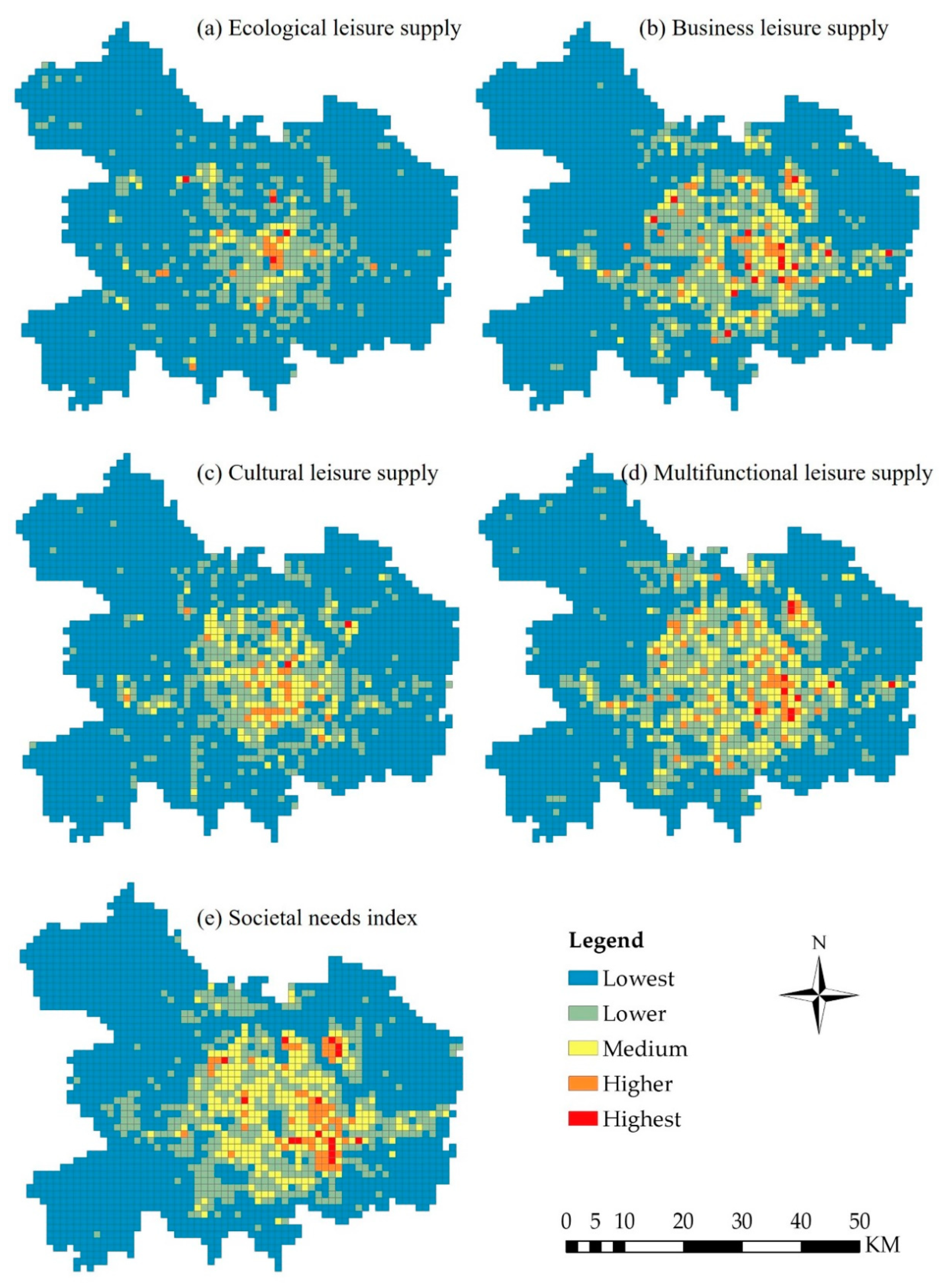
According to the research results, from the perspective of space, the SI of the study area shows that the city center area is higher than the city edges, but the low-value areas are mainly concentrated in the northwestern and southwestern regions. Concerning the types of LSs, the supply of different types can be ranked from high to low as follows: multifunctional services, commercial services, cultural services and ecological services (as shown in Figure 4a,d). The SNI is higher in the center of the study area than at the edges, the value is lower in the west than in the east, and the value is higher in the north than in the south. Dongcheng, Xicheng, Chaoyang and Haidian display significantly higher values than Shijingshan and Fengtai, and the value in Fengtai is the lowest (as shown in Figure 4e). The SI and SNI values in the study area show different spatial distribution trends. Variations in the population, infrastructure construction, population density and economic development level are the main reasons for the different distributions. Infrastructure construction is more developed in high-SI areas than in other areas, thus resulting in more LSs. Areas with large populations, relatively high economic levels, and frequent human activities generally have high SNI value areas and a high demand for LSs.

4.2. Multiattribute Model Analysis

Since our method can calculate the supply and demand of LSs in urban areas, we analyze the accuracy of the model by comparing it with the actual situation (local knowledge base). The reliability and accuracy of spatial mismatch between the supply and demand of urban LSs analyzed using our proposed method may be influenced by the choice of model variables. There are two uncertain variables in this research: traffic hub and GDP density. To obtain different calculation models and optimal attribute combinations, we constructed a three-attribute model, a four-attribute model and a five-attribute model (

Table 2. Different methods involving combinations of models.

ID	Model	L 1	T 2	R 3	P 4	E 5
1	Five-attribute model	√	√	√	√	√
2	Four-attribute model 1	√	√	√	√
3	Four-attribute model 2	√		√	√	√
4	Three-attribute model	√		√	√

¹ L = the ratio of LS POIs; ² T = the ratio of traffic hubs; ³ R = the ratio of residential POIs; ⁴ P = population density; ⁵ E = economic density.

).

For verification, we manually selected one landmark in each region for each category of LS (

Table 3. Comparison of the actual supply and demand and calculated results.

ID	Landmark	District	Leisure Type	Actual Supply and Demand	Model for Validation
					1 1	2	3	4
1	Yuanmingyuan	Haidian	EL	H-L	H-L	H-L	H-H	H-H
2	Temple of Heaven Park	Dongcheng	EL	H-H	H-H	H-H	H-H	H-H
3	Beijing Zoo	Xicheng	EL	H-L	H-H	H-L	H-H	H-H
4	Chaoyang park	Chaoyang	EL	H-L	H-L	H-L	H-H	H-H
5	World Park	Fengtai	EL	H-L	H-L	H-L	H-H	H-H
6	Beijing International Sculpture Park	Shijingshan	EL	H-H	H-H	H-H	H-H	H-H
7	Wukesong	Haidian	BL	H-H	L-L	H-L	L-L	L-L
8	Wangfujing	Dongcheng	BL	H-H	L-H	H-H	H-L	H-L
9	Dashilar	Xicheng	BL	H-H	H-H	H-H	H-L	H-H
10	Sanlitun	Choayang	BL	L-H	L-H	L-H	L-L	L-L
11	Wanda Plaza	Fengtai	BL	L-H	L-H	L-H	L-L	L-L
12	Wanda Plaza	Shijingshan	BL	H-H	L-H	H-H	L-L	L-L
13	Summer Palace	Haidian	CL	H-L	H-L	H-L	H-H	H-H
14	Palace Museum	Dongcheng	CL	H-L	H-L	H-L	H-H	H-H
15	Grand View Garden	Xicheng	CL	H-L	H-L	H-L	H-H	H-H
16	Jiuxianqiao	Chaoyang	CL	H-H	L-H	H-L	H-L	H-L
17	Beijing Garden Expo	Fengtai	CL	H-L	H-L	H-L	H-H	H-H
18	Cultural Center	Shijingshan	CL	H-H	H-H	H-H	H-L	H-L
19	Beijing Sport University	Haidian	ML	L-H	L-H	L-H	L-L	L-L
20	Beijing Workers’ Stadium	Dongcheng	ML	L-H	L-H	L-H	L-L	L-L
21	Beijing Zoo	Xicheng	ML	H-H	H-H	H-H	H-H	H-H
22	National National Olympic Sports Center	Chaoyang	ML	H-L	H-L	H-L	H-H	H-H
23	Nangong Leisure Square	Fengtai	ML	L-L	L-L	L-L	L-L	L-L
24	Shougang Basketball Center	Shijingshan	ML	L-H	L-H	L-H	L-L	L-L
	Model accuracy				79%	92%	17%	25%

¹ The numbers 1, 2, 3, 4 correspond to the ID of the models in Table 2.

) and rely on local knowledge to determine the LS supply-demand pattern. Then, the pattern is compared with the supply–demand patterns calculated by models 1 (five-attribute model), 2 (four-attribute model 1), 3 (four-attribute model 2) and 4 (three-attribute model). We used the accuracy indicator to evaluate the results of these models.

Overall, from Table 3, we learn the following: (1) in descending order of strength, the models with the best ability to calculate supply-demand patterns were the four-attribute model 1, five-attribute model, three-attribute model and four-attribute model 2. (2) For a single attribute, the GDP may reduce the accuracy of the model, while the traffic hub can improve the accuracy of the model.

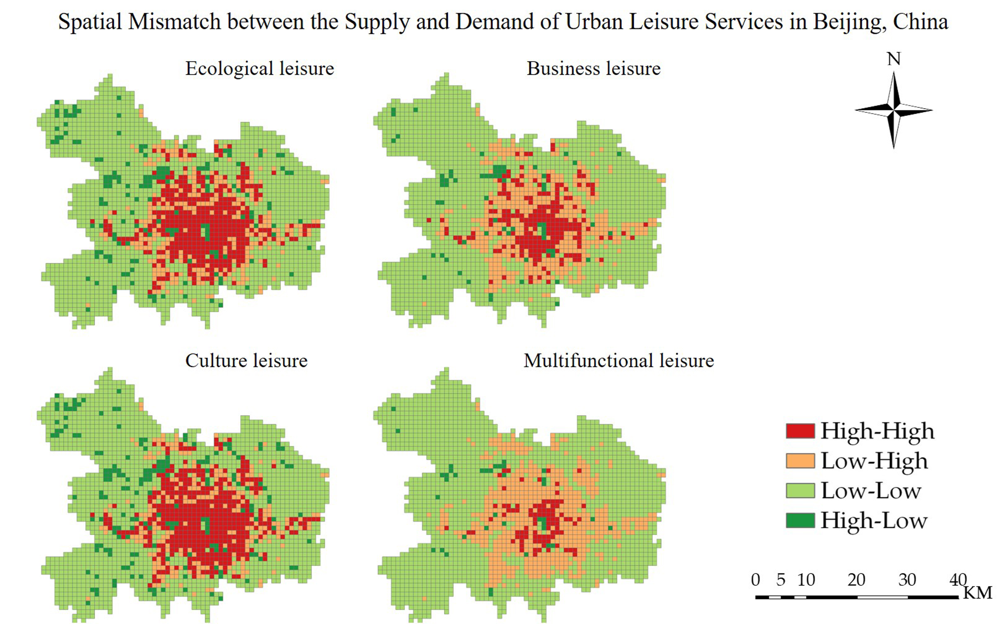
4.3. Spatial Pattern in the Supply and Demand of LSs

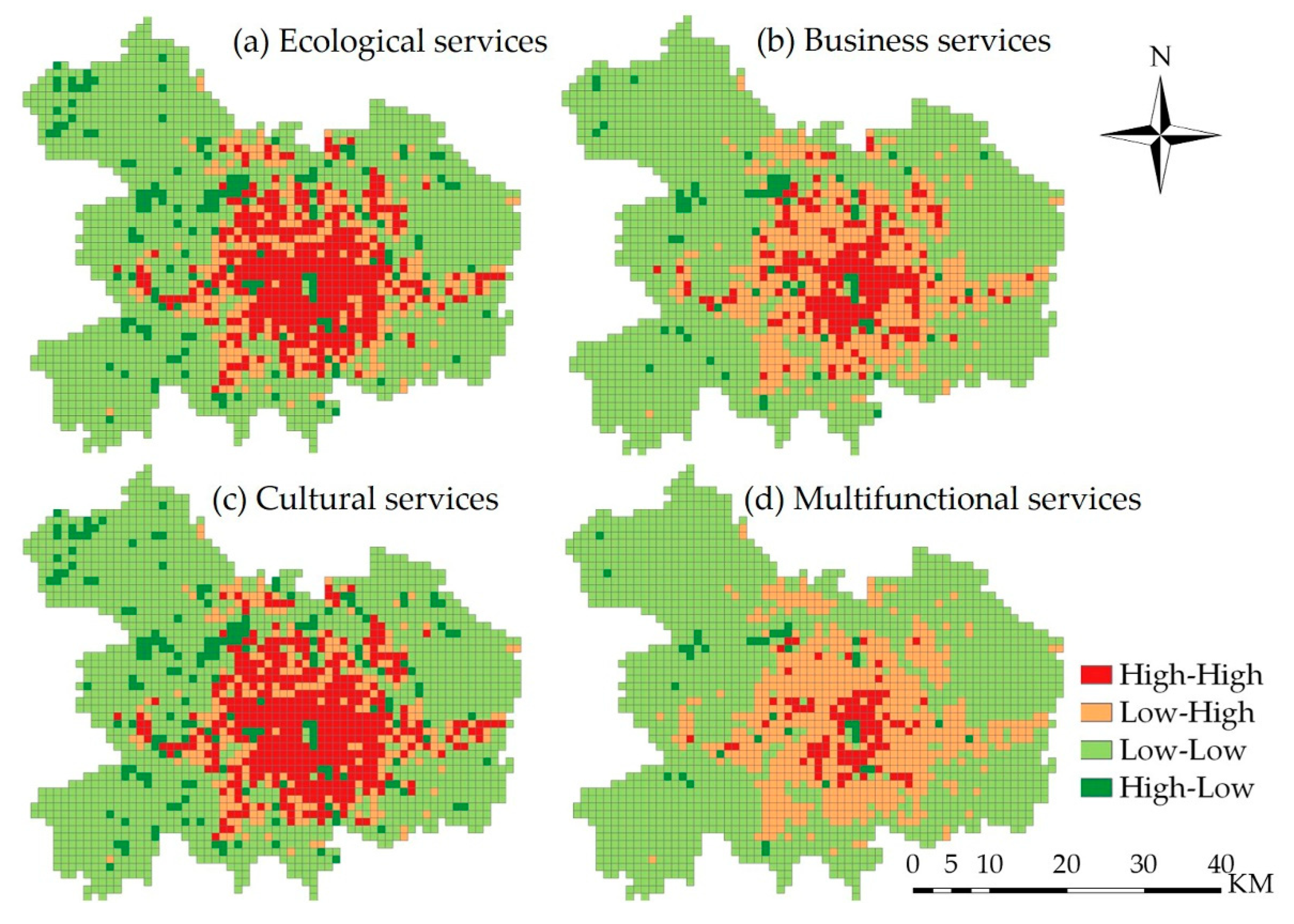
After obtaining the best multi-attribute model (four-attribute model 1), we analyzed the supply and demand pattern (High supply-High demand, Low supply-High demand, Low supply-Low demand and High supply-Low demand) of LSs in the main urban areas of Beijing. Based on the quadrant diagram of the supply and demand of LSs, most regions in Beijing follow the L-L pattern (Figure 5 and

Table 4. Distributions of the numbers of different supply-demand patterns in Beijing, China, 2019.

Type	EL	BL	CL	ML
High supply-High demand	396	211	430	93
Low supply-High demand	276	461	242	579
Low supply-Low demand	1503	1592	1474	1619
High supply-Low demand	154	65	183	38

).

For EL services, the H-H pattern (which was observed in 396 regions) was located mainly in central urban areas, where economic development has advanced and the degree of urbanization was high compared to other regions. The L-H pattern (which was observed in 276 regions) was located mainly between the H-H region and L-L region. Most regions where the L-L pattern was observed were located mainly in the periphery of the city, and a few regions where the H-L pattern was observed were scattered throughout the city (Figure 6a).

For BL services, the supply and demand situation reflects mainly two patterns (L-H and L-L). The number of L-H patterns accounted for 20% of the total number of patterns, and the number of L-L patterns accounted for 68% of the total number of patterns. The L-H pattern was located between the H-H pattern and L-L pattern, and the L-L pattern was located mainly in suburban areas. In addition, the H-H pattern and a small number of regions where the H-L pattern was observed were located in the central areas in the Xidan and Wangfujing commercial centers. As famous commercial streets in Beijing, Xidan and Wangfujing play a significant role in Beijing’s commercial leisure (Figure 6b).

For CL services, the patterns vary mainly as follows from inside to outside the study area: H-L (18.5%), H-H (10.4%), L-H (7.9%) and L-L (63.3%). The H-H pattern was distributed mainly in the central areas of Beijing mainly because the central area, which has a higher cultural leisure supply, has many historical and cultural attractions. Additionally, the population density is larger in the central areas than in other areas and appears to have a higher cultural leisure demand. Additionally, a few regions that display H-L patterns are scattered throughout the central areas and western area. (Figure 6c)

For ML services, the H-H pattern (4%), H-L pattern (1.6%) and L-H pattern (24.9%) were located in the central areas of the city. Among areas displaying the L-L model, the largest proportion (69.5%) was located mostly in the periphery of the city (Figure 6d).

Among the four types of patterns, the L-L pattern (which was located mainly in the periphery of the city) was observed in the most regions. In these regions, the urbanization level was relatively low due to low economic development, and the demand for LSs was also low. The number of H-L patterns was the lowest, and these patterns were located mainly near Tiananmen Square and the western suburbs; the LSs in these regions are abundant, while the population density in these two areas is relatively low. Concerning the type of LSs, the suburbs of Beijing provide mainly EL, but there is a lack of commercial leisure (BL), CL and ML. The situation in the center of the city is the opposite of that in the suburbs.

4.4. Correlation Analysis between the LS Supply and Demand

To effectively study the relationship between the supply and demand of LSs in different regions in Beijing, correlation analysis was used to evaluate the relationship between the SI and SNI in region scale.

Table 5. The correlation coefficients between the supply index (SI) and societal needs index (SNI).

District	EL	BL	CL	ML
Dongcheng	−0.136 *	0.454 **	0.053 *	0.460 ***
Xicheng	−0.302 ***	0.479 **	0.127 *	0.473 ***
Chaoyang	0.3141 ***	0.623 ***	0.400 ***	0.654 ***
Fengtai	0.312 ***	0.707 ***	0.438 ***	0.722 ***
Shijingshan	0.268 ***	0.788 ***	0.441 ***	0.734 ***
Haidian	0.259 ***	0.667 ***	0.515 ***	0.667 ***

* p-value < 0.1; ** p-value < 0.05; and *** p-value < 0.01.

lists the correlation coefficient and significance degree in six regions between the SI and SNI. The results indicate that for BL and ML services, the SI in most regions in Beijing was positively correlated with the SNI, and there was no significant correlation between the SI and SNI in EL and CL services. Especially in Dongcheng and Xicheng, there is no obvious correlation between the supply and demand of all services. For a historical and cultural city such as Beijing, EL and CL services are the foundation of the city, and these services are limitedly affected by urban planning. In addition, urban planning coupled with factors such as different planning objectives, urban structures and economic levels in different regions contribute to the complexity of the relationship between the SI and SNI.

Figure 7 shows the spatial gradients of the LS supply and demand from four directions. The results indicate that there are substantial differences in the LS supply and demand along these axes. In the central urban area, there is a high supply and high demand of LS, while at distances far from the urban central areas, there is a low supply and low demand of LS. Along the W-E axis (Figure 7a), LS demand in Haidian Xicheng and Chaoyang districts is mostly higher than supply, while that in Dongcheng and central Chaoyang districts is lower than supply. Along the N-S axis (Figure 7b), the LS demand in Chaoyang district is much higher than supply, while in Dongcheng district, it is lower than supply. The LS demand and supply in Fengtai district changes from high to low with increasing distance from the urban center. Along the SW-NE axis (Figure 7c), the demand and supply in Xicheng, Dongcheng and the southwest of Chaoyang districts are high, while in Fengtai, they are much lower. Along the NW-SE axis (Figure 7d), LS demand in Xicheng, Dongcheng and Chaoyang districts is higher than supply, while in Fengtai district in the outer suburbs the LS demand is lower than supply. Comparison of the supply and demand in different axes reveals that along the W-E axis and N-S axis, the spatial supply and demand are higher than those along the SW-NE axis and NW-SE axis.

5. Discussion

In urban construction and management, it is important to understand the supply and demand relationship and the spatial distribution of LSs. In this study, LSs were reclassified into four types, EL, BL, CL, and ML, and the LS SI and SNI were used to quantitatively measure the supply and demand of LSs. The SI was employed to depict only the LS supply, which represents a spatial trend of the production of leisure goods and services. The SNI was employed to depict LS demand, which represents the consumption and preference needs of human living. The mismatch analysis on the SI and SNI represents only a relative imbalance in spatial distribution, thereby enabling the rapid interpretation of distribution in the supply and demand pattern of LSs. Moreover, we use the correlation and spatial gradient analysis to characterize the correlations between the supply and demand of LSs in different regions in Beijing. The conclusions of this study differ from those of previous studies and provide a valuable supplement to research on the balanced development of cities.

The results show that there is a positive correlation between the supply and demand of LSs in Beijing, but there are regional and category-based differences in the supply–demand relationship. There is a significant positive correlation between the supply and demand of commercial and multifunctional services, and there is no significant correlation between ecological and cultural services. Thus, the supply and demand of most LSs in Beijing are dependent on urban planning and less influenced by the market economy.

Next, we will discuss the drawbacks of our method and provide policy recommendations.

(1) Superiority of the proposed method

In this study, for the first time in urban research, the concept and classification system for spatial mismatch between the supply and demand of urban LSs is proposed. Considering the limited data on urban LS research, we developed an effective method for identifying the spatial distribution of the urban LS supply and demand from multisource socioeconomic data. First, our method was less time consuming and more cost effective than detecting distributions in absolute values and material goods of LSs by using field survey datasets. The analysis method is meaningful for rapidly detecting and managing LSs. Second, our method can not only detect the spatial distribution of the urban LS supply and demand but also perform correlation analysis, which enables us to quantitatively analyze the relationship between the supply and demand of LSs in urban areas. In addition, research at the grid scale can be easily translated to other research scales, thus making the approach convenient for planners to develop policies at different scales.

(2) Limitations of the proposed method

Although our approach can detect the spatial mismatch of LSs in a given urban area, there are limitations. (1) Limited data availability: this study uses only population data to characterize LS demand, with few indicators selected and a lack of individual preference data, such as residents’ sex and age; therefore, the method may be unable to comprehensively reflect LS demand. For example, the elderly population prefers park leisure, and the young population prefers shopping mall leisure. (2) The supply and demand capacities are represented only by the quantity of each type of LS without considering the different supply and demand capacities that different types of POIs can represent. For example, a large park may have a stronger LS capacity than a small gym. (3) Currently, research on the supply and demand of urban LSs is relatively rare, so there is no effective data comparison. In the future, questionnaires, sampling surveys and field observation data can be used in a small range to improve the verification and accuracy of the model.

(3) Policy recommendations

The spatial imbalance of the LS supply and demand may lead to a series of fairness and justice problems to a certain extent; for example, an area with a balanced level of LS supply and demand or an area with an excess LS supply may make residents happier than those in an area where the demand is not satisfied. In addition, the supply and demand of urban LSs is not equal, and the increase in commuting for entertainment may cause a serious traffic burden. Thus, future urban research should include social and environmental inequity in the analysis of the imbalance between the supply and demand of urban LSs and explore ways to solve the problems related to the distribution of urban leisure benefits. Moreover, urban land use planning should consider the distribution of urban LSs at different scales so that balanced LSs can be provided to residents while meeting economic development objectives.

6. Conclusions

Currently, the main contradictions in Chinese society have been transformed into contradictions between people’s increasing need for a better life and unbalanced and inadequate development. To achieve sustainable economic and social development, policy makers must consider the best way to meet people’s growing needs for a better life in specific decision-making processes. In this study, it is possible for us to quickly display the supply and demand of LSs in different parts of an urban area by using multisource open data and deriving the spatial distribution of areas of mismatch. The results show that most areas in Beijing display high demand-low supply and low supply-low demand patterns for LSs. In addition, this study makes an important attempt to quantify the relationship between the supply and demand of urban LSs. The results can guide urban construction management and decision-making. Overall, we believe that the advantages of this method are its low cost and broad applicability.

Future work should, consequently, focus on the following tasks: (1) improving the accuracy of experimental data, (2) weighing various types of POIs, and (3) considering residents’ personal leisure preferences. These improvements will contribute toward accurately determining the spatial mismatch and distribution of LSs in urban areas.