An Open-Source Framework of Generating Network-Based Transit Catchment Areas by Walking


1
Chair of Cartography, Technical University of Munich, 80333 Munich, Germany
2
School of Geospatial Information, Information Engineering University, Zhengzhou 450052, China
*
Author to whom correspondence should be addressed.
ISPRS Int. J. Geo-Inf. 2020, 9(8), 467; https://0-doi-org.brum.beds.ac.uk/10.3390/ijgi9080467
Submission received: 3 July 2020
/
Revised: 18 July 2020
/
Accepted: 20 July 2020
/
Published: 22 July 2020
Abstract
:The transit catchment area is an important concept for public transport planning. This study proposes a methodological framework to generate network-based transit catchment areas by walking. Three components of the framework, namely subgraph construction, extended shortest path tree construction and contour generation are presented step by step. Methods on how to generalize the framework to the cases of the directed road network and non-point facilities are developed. The implementation of the framework is provided as an open-source project. Using metro stations in Shanghai as a case study, we illustrate the feasibility of the proposed framework. Experiments show that the proposed method generates catchment areas of high geospatial accuracy and significantly increases computational efficiency. The open-source program can be applied to support research related to transit catchment areas and has the potential to be extended to include more routing-related factors.
1. Introduction
The transit catchment area (TCA) is an important concept for transport planning, especially for public transit planning. The catchment area of a transit station can be defined as a geographical area where the majority of passengers will typically be found [1,2]. In recent years, an upsurge of interest has been witnessed in the research on TCAs, including TCA modeling [1,3] and TCA analysis [4,5], which have shown that an in-depth understanding of a TCA can facilitate planning in several aspects. First, a well-defined TCA can support the design of road networks, land uses, and floor area ratios around transit stations [6,7,8]. Second, the TCA is one of the fundamental elements for transit-ridership modeling [9,10,11]. This is because several potential ridership-related factors, such as population, employment, and road quality, are commonly measured based on the catchment area of a station. Third and more generally, the analysis of the TCAs of a certain type of transit system can provide insights into the balance between its supply and demand [12,13,14]. For example, an investigation of the coverage of metro catchment areas can help planners to determine underserved and overserved areas of the metro system and thus support the planning of new metro stations.
The TCA can be classified into different types according to the feeder mode of transit stations. Specifically, the feeder mode can be walking, biking, bus riding and car driving. Walking is generally recognized as the largest feeder mode for several types of transit systems (e.g., urban metro systems); hence, most researchers have reached general agreement that the size of the catchment area of transit stations should be defined for pedestrian access [15,16,17] (known as pedestrian catchment areas). It is thus not surprise to see that most of the previous studies have been focusing on the analysis of TCAs by walking [15,16,17,18,19,20].
Generating an appropriate TCA is one of the prerequisites of the TCA analysis (e.g., coverage analysis). The methods of generating TCAs largely depend on how the TCAs are modeled (i.e., how to represent a TCA). Generally, the modeling of TCAs can be classified into two major categories. The first category represents the catchment area of a transit station as a buffer area around the station, referring to an area within which the majority of users can be located. The size of the buffer area is commonly determined based on passengers’ “acceptable” access/egress travel time/distance. For example, one-half mile is commonly used as the buffer distance to define the rail-transit catchment areas by walking [21]. The buffer distance can be either measured by the Euclidean distance or the network distance. According to [5,22], the latter can generate a more accurate catchment area because people need to travel along roads in the real world. The Euclidean buffer-based method usually overestimates the size of catchment areas because of the detour nature of real roads. The second category can be termed as probability-based TCA modeling, where a catchment area is commonly represented by a set of sub-areas with corresponding probabilities [1,3,23]. This type of TCA modeling is tightly correlated with station choice modeling and usually used for modeling TCAs by motorized transport. For instance, Lin et al. proposed an enhanced huff model to measure the probabilities of train station choice for park-and-ride users living in different suburbs [1]. The derived station choice probabilities are used to redefine the origins of each train station and thus the catchment area of each train station is constructed based on the redefined origins.
Serval studies have discussed how to generate buffer-based TCAs [24,25,26]. The Euclidean buffer-based TCAs can be easily generated by creating a circular area centered at the transit station. By combining the Thiessen polygons and the Euclidean-based buffer areas of transit stations, mutually exclusive polygons can be generated to represent non-overlapped catchment areas [24,26]. With respect to generating buffer-based TCAs along the road network, there are two types of input data model, namely the raster data model and network data model [25]. As for the raster data model, a study region is represented by a tessellation of cells (e.g., square cells). In order to measure the distance along the road network, additional strategies are needed to integrate the road network information into the raster data model. For example, Upchurch et al. proposed a strategy that assigns different weights to network cells (i.e., cells that represent roads) and off-network cells [26]. By setting a “large” weight to the off-network cells, the pathfinding algorithm can guarantee the obtained shortest paths are constrained to the road network. Additionally, areas without road network (i.e., off-network areas) were explicitly represented as off-network cells and thus provide an easy way to measure off-network distances. The accuracy of the TCAs obtained by the raster data model largely depends on the cell size. A smaller size of the cell usually generates more accurate catchment areas because more details, such as the turns of roads, can be modeled in the raster data model. However, a smaller size means a larger number of cells, which could increase exponentially computation time [26]. In contrast, a large size of the cell can help accelerate the computation process at the cost of accuracy.
On the other hand, generating TCAs based on the network data model is a much more straightforward approach because the roads are normally represented as a network data model. No additional data transform between the network data model and the raster data model is needed. The distance along the road network can be accurately measured based on the network data model. As a result, this method is frequently applied to build catchment areas in practice. However, very few studies have been reported on the methods of generating TCAs based on the network data model (termed network-based TCAs). Most of the existing studies [5,13,25,27] mentioned that the network-based TCAs are generated using the service area tool of ArcGIS [28]. However, few studies have discussed how to generate the network-based TCAs and how to evaluate their accuracy. Although a study [25] showed that the catchment areas based on the raster data model tend to overestimate the coverage as compared with those based on the network data model, a quantitative evaluation on the accuracy of the network-based catchment areas is still missing.
In recent years, the rising importance of open-source approaches in geospatial analysis and visualization has been widely recognized for two major reasons [29,30,31]. First, open-source approaches provide an easy way for researchers to re-conduct similar analyses without worrying about software and/or data limitation. Second, since open-source approaches are fully transparent, the corresponding algorithms and workflows can be better understood and revised/extended in a flexible way. Following this direction, we herein focus on proposing an open-source framework of generating network-based TCAs by walking. In addition, we aim to develop a method to evaluate the geospatial accuracy of the network-based TCAs. The contribution of this work regards the following three aspects.
- We propose a methodological framework to generate the network-based TCAs by walking.
- We propose a method to evaluate the geospatial accuracy of the network-based TCAs.
- We provide an open-source implementation of our framework.
The rest of the paper is organized as below. In Section 2, we first present the methodological framework of generating the TCAs by walking. Then, we propose a metric to evaluate the geospatial accuracy of the catchment area. Section 3 showcases our framework by generating the catchment areas of metro stations in Shanghai as case studies, followed by the evaluation of geospatial accuracy and time efficiency. In Section 4, we discuss the limitation and potential extension of the proposed framework and we conclude the study in Section 5.
2. Methods
2.1. Problem Definition and Assumptions
Given a road network graph (where the node set N represents road intersections and the edges set E represent the corresponding roads) and a transit facility with a cut-off distance , the network-based catchment area of is defined as an area that exactly encompass all the points with a distance to no longer than . We refer the points within the delta distance of as the accessible points and points beyond this distance as inaccessible points. The “exactly” means that all the inaccessible points should be excluded in the catchment area. The distance between a point and a facility includes two parts: network and off-network distances. Two assumptions are made to facilitate the distance measurement. First, users are assumed to choose the nearest road of the origin/destination to start/end their traveling along the road network. Second, users are assumed to choose the shortest path to travel along the road network. Based on these two assumptions, the network and off-network distances can be measured and the distance between and any point can be obtained accordingly. The shortest path may not always be the optimal route, factors such as time, familiarity, and number of turnings can also affect users’ route choices. However, since these factors can be converted to distances with a weighting function, the assumption of the shortest path still holds in a general sense (see Section 4 for more details).
Based on the definition of the network-based TCA, the problem under consideration is described as:
Given a road network graph and a set of facilities . Each facilityhas an associated cut-off distance . The aim is to design a method to generate n TCAs for these facilities in an efficient and accurate way.
The “efficient” here means the method should be fast in terms of generating a large number of catchment areas. The “accurate” means the generated catchment area should match with the TCA definition as much as possible, i.e., the generated catchment area should include more accessible points and fewer inaccessible points (see Section 2.4 for the detailed evaluation metrics).
2.2. Framework of Generating Network-Based Transit Catchment Areas (TCAs)
The catchment areas can be measured in two directions, namely to-facility and from-facility directions, corresponding to using the facility as the destination and origin, respectively. For undirected road networks, the distance measured in to-facility direction is the same as that measured in from-facility direction; thus, the to and from facility catchment areas are the same. In contrast, it is necessary to differentiate the to-facility and from-facility catchment areas for the case of the directed road network. In addition to representing a facility as a point, the facility can also be geometrically represented as a set of points (i.e., multiple points), a polyline, or a polygon. In this section, we focus on illustrating the framework of generating the TCAs by walking using the case of the undirected road network and point-based facility. The methods on how to generalize the framework to directed graph and non-point facility are described in Section 2.3.
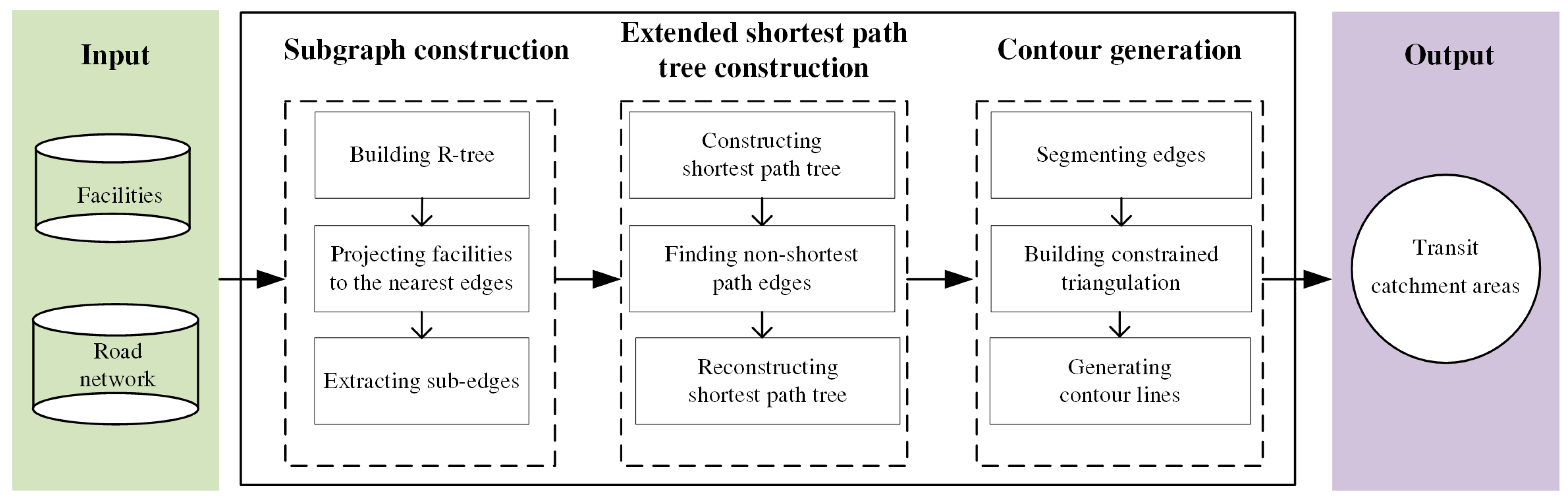
Figure 1 illustrates the workflow of the proposed framework. The general idea is to build a triangulation to interpolate the contour at the cut-off distance, and the area enclosed by the contour is used as the catchment area. Specifically, given the input road network and facilities, the workflow includes three components: subgraph construction, extended shortest path (SP) tree construction, and contour generation. We elaborate on these three components in the following subsections.
2.2.1. Subgraph Construction
Since the cut-off distances for TCAs based on walking are generally small, a subgraph is constructed for each facility to accelerate the construction of extended shortest path tree (see Section 2.2.2) by limiting the shortest path searching to a small size of subgraph (i.e., graph with fewer nodes).
- Building R-tree. Based on the input road network edges, an R-tree [32] is built to accelerate the nearest road searching and sub-edge extraction.
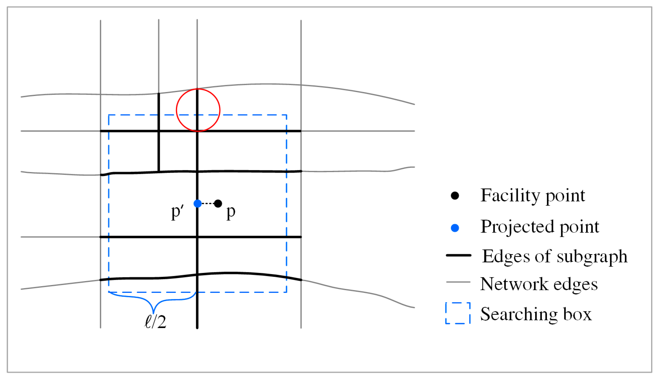
- Projecting facilities to the nearest edges. In order to measure the distance from/to a facility, each facility point is projected to its nearest edge. The nearest edge of a facility is retrieved using the nearest neighbor query of R-tree [33]. Then, each facility is projected to its nearest edge by using a linear reference algorithm, which iterates through every segment (i.e., a line connecting two neighboring points of an edge) of the edge to determine the nearest segment [34]. As illustrated in Figure 2, is the corresponding projected point of the facility.
- Extracting sub-edges. Based on the projected points obtained, a set of edges around each projected point can be identified. Given a facility with its projected point and the cut-off distance, a square searching box with a width of and centered at is created (Figure 2). The sub-edges of each facility are then extracted by finding the edges that intersect with its searching box with the assistance of the intersection query of R-Tree. Based on the extracted sub-edges of each facility, the corresponding subgraph for a facility can be constructed. Additionally, the projected point is inserted into as a new node. The parameter setting of needs to satisfy two requirements: (1) all the accessible edges (i.e., edges whose distance to/from are less than or equal to should be included in ; and (2) some edges beyond the distance of need to be included in , which will be used to interpolate additional boundary points of the catchment area (see Section 2.2.3). Therefore, should satisfy the following formulawhere is the Euclidean distance between and , is the given cut-off distance of . Under the condition of these two requirements being satisfied, should be as small as possible to improve the computation efficiency. We set to be for three reasons. First, the detour ratios of roads are generally bigger than 1. Second, is usually bigger than 0. Third, boundary edges with distances to larger than are naturally included in the subgraph because we use the “intersection query” to extract sub-edges (e.g., the edge marked by the red circle in Figure 2).
2.2.2. Extended Shortest Path Tree Construction
An extended shortest path (SP) tree is constructed for each subgraph, based on which the distance from a node to any point along the road network can be measured [35].
- Constructing SP tree. Given a node as the root node, the SP tree starting from a root node can be constructed by employing Dijkstra’s algorithm.
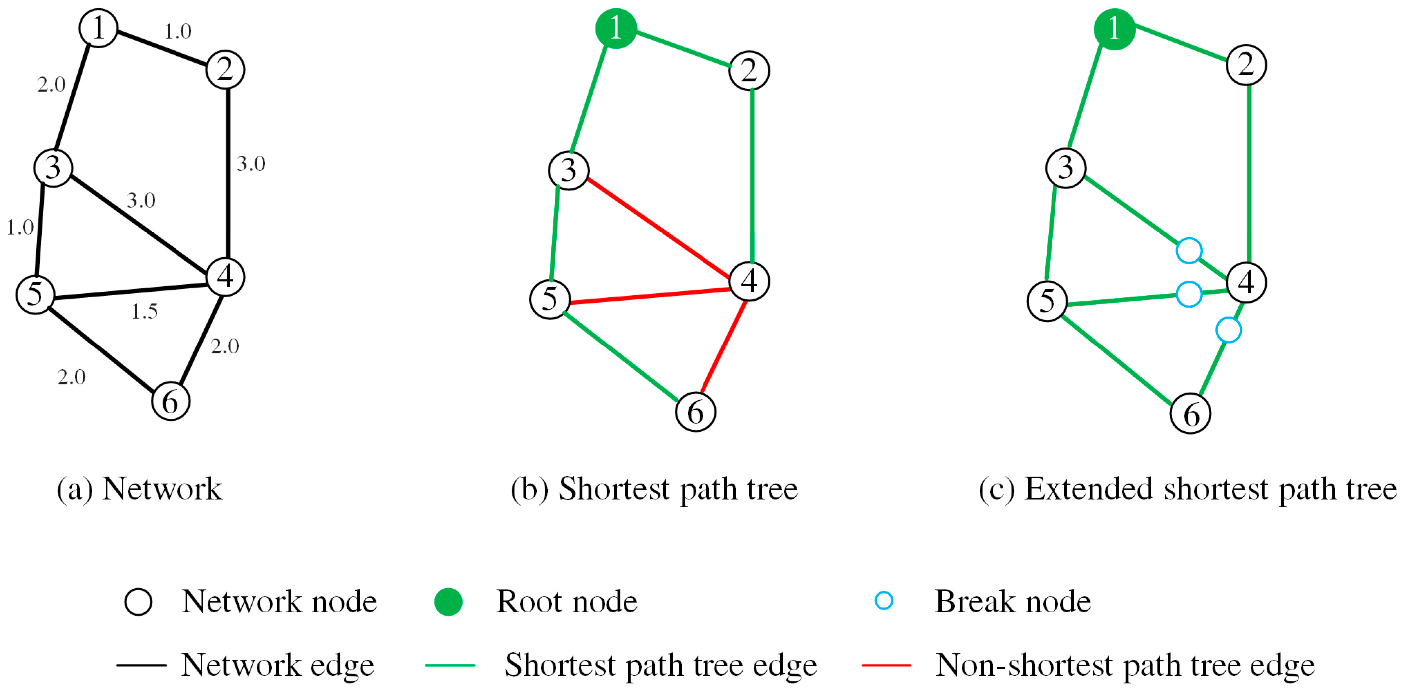
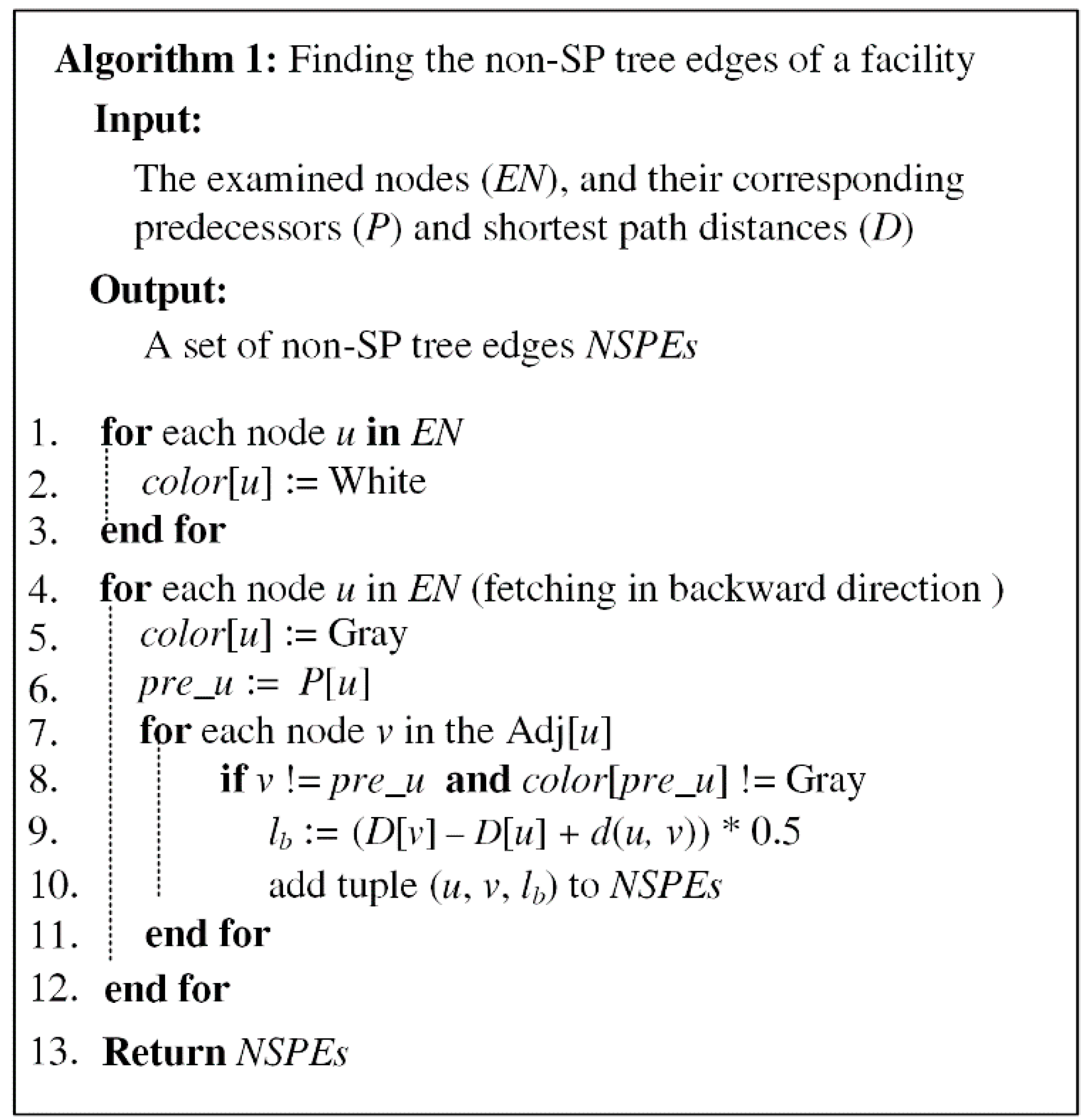
- Finding the non-SP tree edges. As illustrated by an example in Figure 3. Some edges (the red edges in Figure 3b) are not included in the SP tree, which are termed non-SP tree edges. In order to construct an extended SP tree that includes these non-SP tree edges, we need to insert additional points into them. According to [36], if a given edge is a non-SP tree edge, there must be a point (termed as break point) on this edge that satisfies the following:where are the network distances from the root node to nodes and , and are the network distances between point and nodes and . How to efficiently find the non-SP tree edges and the corresponding break points is the key issue of constructing the extended SP tree. We represent a non-SP tree edge as a tuple , where . Algorithm 1 describes the means of identifying the non-SP tree edges of a facility (denoted as , see Figure 4). The input of this algorithm is the output of the Dijkstra’s algorithm (i.e., the output of the preceding step), including the sequence of the examined nodes of the Dijkstra’s algorithm (denoted as ), the predecessors of the examined node (denoted as), and the shortest distances of the examined nodes to the root node (denoted as ). By iterating the examined nodes in a backward direction, the non-SP tree edges can be efficiently identified (Lines 4–12 in Algorithm 1).
- Reconstructing SP tree. Each non-SP tree edge is split into two edges at its break point , namely edge and edge . Although and have the same location, there are regarded as two distinct nodes to avoid circular roads in the graph after inserting the break points [36]. After the insertion of every single non-SP tree edge, an updated graph can be obtained. Then, by re-running Dijkstra’s algorithm on this updated graph, the corresponding extended SP tree can be generated (Figure 3c).
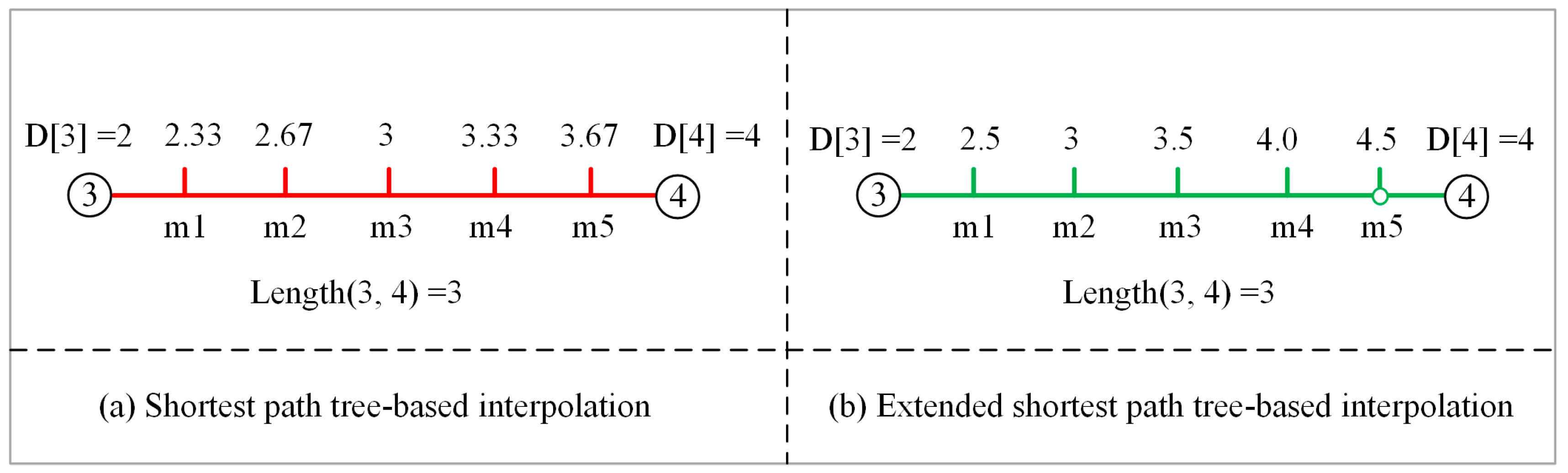
Compared with the SP tree, the extend SP tree can include all the non-SP tree edges. The inclusion of these edges is essential for the distance interpolations during the contour generation (see Section 2.2.3). Figure 5 illustrates the interpolations based on the SP and extended SP trees by using a non-SP tree edge (i.e., edge (3, 4)) from Figure 3b). As demonstrated, if no break point (i.e., in Figure 5b) is inserted, the interpolation along the edge is incorrect. For instance, the distance from the root node to point is 2.5. Under the condition of the extended SP tree, the distance to can be correctly determined through the interpolation along the (see Figure 5b). Under the condition of the SP tree, the distance is wrongly determined as 2.33 if the interpolation is conducted along the (see Figure 5a). Since a non-SP tree edge might be used as an edge of the triangulation, it is essential to build the extend SP tree to guarantee a correct interpolation during the triangulation.
In the context of the TCA generation, the root node of the extended SP tree is set to be the projected point . The network corresponds to the subgraph of the facility. By following the above three steps, an extended SP tree can be generated for each subgraph.
2.2.3. Contour Generation
Based on the extended SP tree constructed in Section 2.2.2, the contour lines at the distance is generated for a facility as the boundaries of its catchment area in the following three steps.
- Segmenting edges. Given an edge represented by point sequence, where to are intermediate points of edge . We divide the edge into segments and add them as constraints during the triangulation (their endpoints thus act as the vertices of the triangulation). Since every single edge is included in the extended SP tree, the distance from a root node to an intermediate point can be calculated by the following formula.where is the distance from the root node to the intermediate point , is the distance from the root node to node , is the distance from node to the intermediate point .
- Building constrained triangulation. Based on the constrained segments obtained in the previous step, a constrained Delaunay triangulation is built for each extended SP tree by using the Computational Geometry Algorithms Library [37].
- Generating contour lines. Using the constrained triangulation as input, the contour lines specified at the cut-off distance (i.e., ) are generated by employing a tracing-based contour generation algorithm [38].
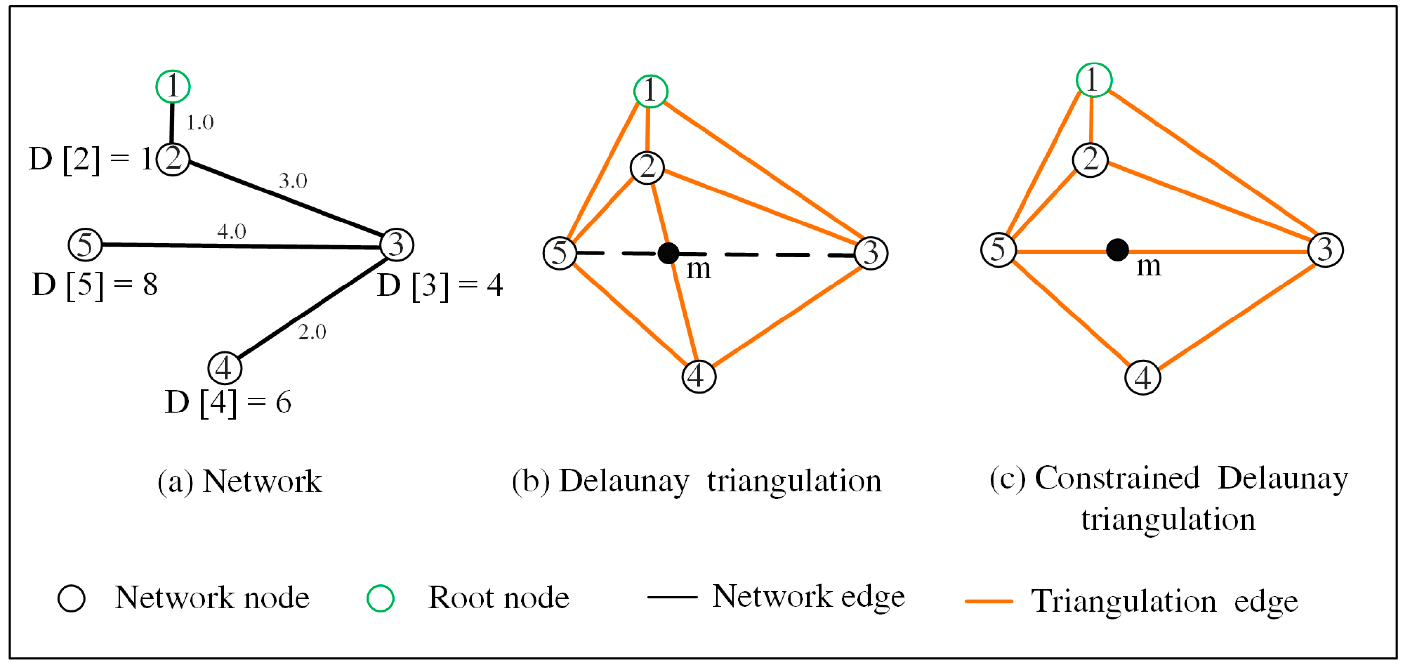
We build the constrained Delaunay triangulation instead of normal Delaunay triangulation because the edges of Delaunay triangulation may intersect with network edges and lead to incorrect distance interpolation during the contour generation. Figure 6 shows an example of the Delaunay and constrained Delaunay triangulations for a road network. Figure 6b shows a triangulation edge (2,4) intersecting with a network edge (3,5) at point m. In such case, the distance from the root node to point m is interpolated based on the triangulation edge (2,4) because the network edge (3,5) is not a triangulation edge. As a result, the interpolated distance is different from the real distance from node 1 to point m (following a path 1–2–3–m). In contrast, since every network edge is included in the constrained Delaunay triangulation (Figure 6c), the distance from the root node to any point along the network edge can be correctly measured.
2.3. Generalization of the Framework
In Section 2.2, we illustrate our framework using the case of the undirected road network and point-based facilities. In this section, we present the methods on how to generalize the framework to the cases of the directed road network and non-point facilities.
2.3.1. Generalization to the Directed Road Network
The major differences between the directed and undirected road networks occur at the process of “Extended shortest path tree construction”. Three modifications need to be made.
First, for the directed graph, the adjacent nodes in Line 7 of Algorithm 1 specify the start nodes of the in-edges (i.e., edges with the target node at node u) of node u. Whereas for the undirected graph, there is no need to distinguish the in-edges and the outer-edges of a node.
Second, if an edge corresponds to a single-direction road edge is a non-SP tree edge, we must have . Then, it is only possible to find a point at the location of that satisfies formula (2). Therefore, there is no need to insert any break point under such conditions. Although no break point is added into a non-SP tree edge when it corresponds to a single-direction road edge, during the segmentation of road edges (see Section 2.2.3), the distance between an intermediate point and the root node can also be determined using formula (3).
Third, during the reconstruction of the shortest path tree, both edges (i.e., edge () and edge ()) of a bi-direction edge need to be split at the break point . Additionally, instead of inserting two points (i.e., and ) with same location, only one break point needs to be inserted.
As noted in Section 2.1, the to and from facility TCAs are different for the directed road network. By default, the root node of Dijkstra’s algorithm is set to be the projected facility point, which corresponds to the from-facility catchment area. With respect to the generation of the to-facility catchment area, the only modification is to reverse the direction of each edge during the construction of subgraph (Section 2.2.1). Then, by using the projected facility point as the root node, the derived catchment area can be changed from the “from-facility” catchment area to the “to-facility” catchment area.
2.3.2. Generalization to Non-Point Facilities
Since polylines and polygons can be transferred into a set of multiple points by using a discretization strategy, we use the case that a facility is represented as by a set of multiple points to illustrate how to generate the catchment areas for non-point facilities. This is assuming a facility is represented by sub points ), and their corresponding projected points are . An intuitive method of generating the catchment area of is to dissolve all the individual catchment areas of its sub points (termed as dissolving-based method). We herein propose another method, termed as virtual node-based method, to generate the catchment area of in a more efficient way. Specifically, the virtual node-based method requires two modifications.
First, during the processing of subgraph construction, the searching box should be set as the bounding box of all the searching boxes of .
Second, a virtual node needs to be added into each subgraph during the subgraph construction. The weights between the virtual node and any of point in . are set to be zero. Then, this virtual node is used as the root node to construct the extended SP tree and generate the corresponding catchment area.
2.4. Geospatial Accuracy Metrics
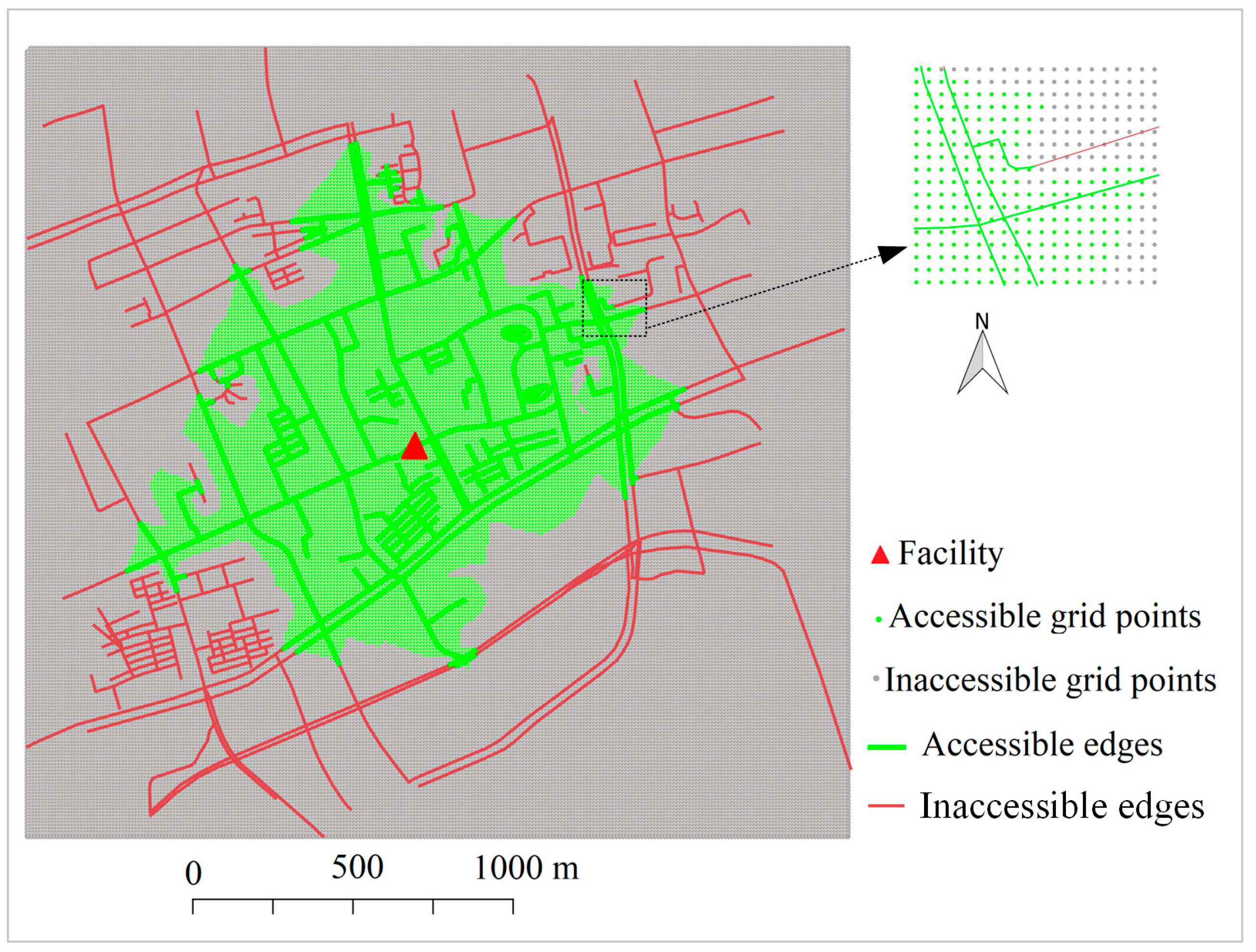
For the evaluation of the geospatial accuracy of a catchment area, a benchmark is needed to represent the “correct” catchment area of a facility with a given cut-off distance. Corresponding to the TCA definition given in Section 2.1, a set of regular grid points within the searching box of each facility are generated (see Figure 7). The distance between a grid point and the facility can be measured based on the extended-SP tree and then classified as an accessible or inaccessible point. Theoretically, a good catchment area should satisfy two criteria (1) a high ratio of the correctly included accessible points to all the included points, and (2) a high ratio of the correctly included accessible points to the all accessible points. Thus, the accuracy evaluation of catchment areas can be deemed to be the evaluation of a binary classification issue. Specifically, the first criterion means a high precision; and the second criterion means a high recall. Furthermore, another commonly used integrated metric, i.e., F1 score, is used as an integrated metric of the accuracy evaluation. F1 score is the harmonic average of the precision and recall, and a higher F1 score represents a better accuracy of the generated catchment area. Mathematically, the precision, recall and F1 score are measured as follows.
where denotes the number of accessible grid points within the catchment area, denotes the number of grid points within the catchment area, . denotes the number of accessible grid points, . denote the precision, recall, and F1 sco, respectively.
2.5. Implementation
The proposed framework is implemented as an open-source C++ program (https://gitlab.com/Drsulmp/tcageneration). The program can be used to generate catchment areas with different configurations. Specifically, the input road network can be undirected roads or directed roads; the input facilities can be point-based or multiple points-based facilities. Additionally, the program also provides function to generate accessible edges within the TCAs.
3. Case Study and Evaluation
In this section, we first conduct case studies to validate the feasibility of our framework. Then, we conduct several experiments to evaluate the accuracy and time efficiency of the proposed method.
3.1. Data Description and Experimental Set-up
Two major datasets, namely metro station dataset and road network dataset, are prepared for experiments. The metro station dataset includes 1223 metro station entrances of 301 metro stations in Shanghai, which are collected via Gaode map API (a leading map service in China). The road network of Shanghai is downloaded by using the OSMNX python package [39]. The road network is modeled as an undirected graph. All the experiments are conducted on a desktop computer with Intel Quad Core central processing unit (CPU) 3.40 GHz and 32 GB RAM.
3.2. Case Study
3.2.1. Undirected Graph with Point-Based Facility
Using the Da Muqiao metro station as an example, the process of catchment generation is shown in Figure 8. In this example, the road network is represented as an undirected graph, the station is represented as a point. The cut-off distance and the width of the searching box are set to be 1 km and 2 km, respectively. Figure 8a shows the sub-edges extracted by using the searching box. Figure 8b shows the SP tree and non-SP tree edges among the sub-edges. As indicated, all the non-SP tree edges and their corresponding break points are successfully extracted using Algorithm 1. Figure 8c shows the constrained Delaunay triangulation. The intermediate points and segments are included in the triangulation as its vertices and edges, respectively. Figure 8d shows all the accessible edges and the corresponding catchment area. The catchment area is represented by a polygon consisting of an exterior ring and three interior rings (i.e., the “holes” in Figure 8d), corresponding to four obtained contours lines. Obviously, all the accessible edges are successfully covered by the generated catchment area. Moreover, the inaccessible areas within the exterior ring can be identified and excluded in the generated catchment area.
3.2.2. Directed Graph and Non-Point Facilities
For the case of the directed graph, several bi-directional edges in Figure 8a are modified into single-direction edges (the red edges in Figure 9) to construct a directed subgraph. Figure 9 shows the generated catchment areas in to and from facility directions using the same cut-off distance as that of Figure 8. Although only a few edges are modified as single-direction edges, a distinctive difference is observed between the results for the undirected graph (Figure 8d) and the directed graph (Figure 9a). Additionally, we determine that the dissolved areas of the from-facility (Figure 9a) and to-facility (Figure 9b) catchment areas of the directed graph is almost the same as the catchment area generated by the undirected graph (Figure 8d). This is because the input directed graph for the to-facility catchment is obtained by reversing the directions of roads of the from-facility catchment area.
Figure 10 shows the catchment area of a multiple-point facility. In this example, Da Muqiao metro station is represented by its six entrances. The cut-off distance is set to be 1 km. The catchment area boundaries of each individual metro entrance by using 1 km as the cut-off distance are generated as well (in yellow dotted lines). As shown in Figure 10, the generated catchment area of the multiple-point facility is almost the same as that obtained by dissolving the individual catchment areas of each entrance. This demonstrates that the virtual node-based method can be effectively applied to generate catchment areas for non-point facilities.
3.3. Geospatial Accuracy Evaluation
3.3.1. Visual Comparison
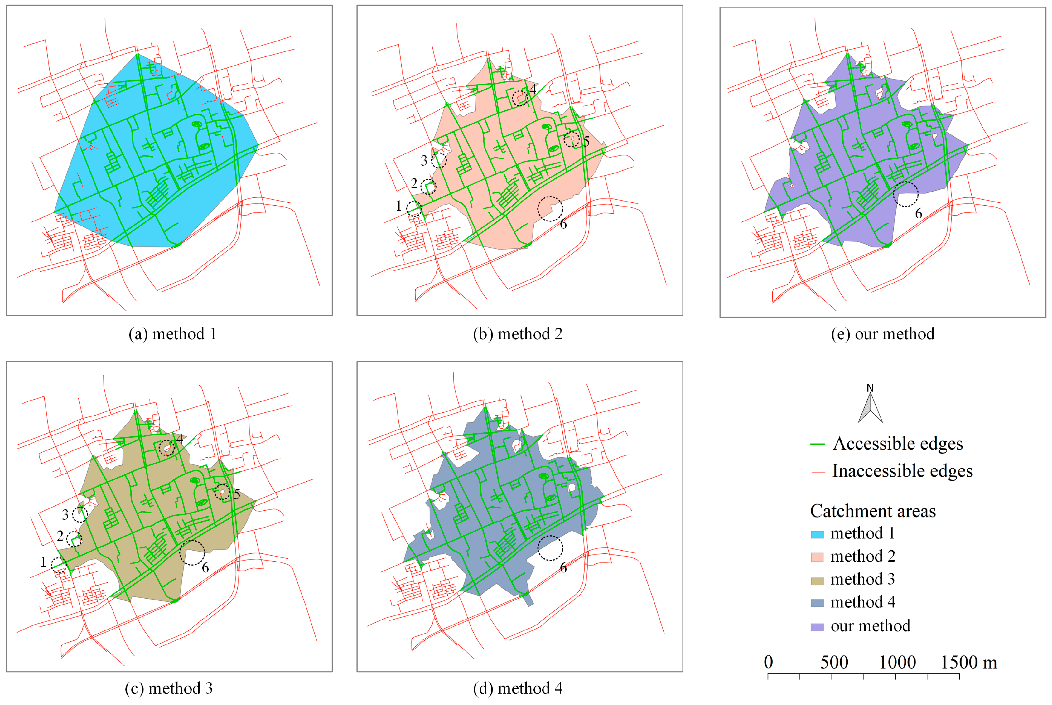
To illustrate the effectiveness of the proposed method, four alternative methods are compared.
Method 1: Convex hull-based method. This method first finds the cut-off points along with the network, whose distances to/from the facility are equal to the cut-off distance. Then, the convex hull of the cut-off points is used as the catchment area.
Method 2: A SP tree-based triangulation method. This method is a simplified version of the proposed method. Specifically, after the construction of subgraph, a normal SP tree is built to obtain the distances between network nodes and the facility. Then, using the network nodes as the input, a Delaunay triangulation is built to generate the contour lines at the specific cut-off distance.
Method 3: An extended SP tree-based triangulation method. As indicated by the name of this method, the difference between this method and the proposed method only occurs at the part of triangulation construction. Instead of a constrained Delaunay triangulation, a Delaunay triangulation is constructed. The contour lines are then generated based on the constructed Delaunay triangulation.
Method 4: The ArcGIS method. In this method, the service area tool provided by ArcGIS is used to generate the network-based catchment areas. The ArcGIS method is conducted via the ArcGIS Desktop 10.6, where the polygon type of the service area is set to be “detailed” and the other parameters are set as default.
Using the same input and setting as that of Section 3.2.1, the catchment areas generated by the four above methods and our method are visualized in Figure 11. It is noticeable that some inaccessible edges are wrongly included in the catchment area generated by method 1. Very few inaccessible edges are wrongly included in the catchment areas generated by method 2 and 3. As shown by the dotted black circle 4 in Figure 11c, the method 3 has improvements on excluding inaccessible edges than method 2 because the non-SP tree edges are included in the extended SP tree. Some accessible edges are not correctly included in the catchment areas generated by method 2 and 3. Specifically, these accessible edges are marked by the dotted black circles 1, 2 and 3 in Figure 11b,c. In contrast, all accessible edges are correctly included, and inaccessible edges are correctly excluded in the catchment areas generated by method 4 (Figure 11d) and our method (Figure 11e). Slight differences can be found in terms of the shapes of these two catchment areas (e.g., marked by the dotted black circle 6 in Figure 11d,e). The comparison between our method and method 3 illustrates the necessity of building the constrained Delaunay triangulation. The comparison between method 3 and method 2 shows the advantages of the extended SP tree over the SP tree.
3.3.2. Quantitative Evaluation
In this section, the geospatial accuracy of TCAs generated by the proposed method is evaluated quantitatively. Based on the visual analysis of in the preceding section, the ArcGIS method is selected as a comparison because it has the results closest to ours (see Table 1). For evaluation, of the 32 station centers of the metro line 12 are used as the input facilities. Corresponding to the pedestrian access, the cut-off distances are set to be 0.8 km, 1 km, and 1.2 km, respectively (see [40] for a review of walking distances to transit). The size of the grid is set to be 10*10 m for the generation of grid points. Given a cut-off distance, we can measure the corresponding precision, recall and F1 score for each station. The average values of the precision, recall and F1 score of the 32 stations are listed in Table 1. As indicated by the average number of grid points in the TCAs, the TCAs generated by our method are larger than those generated by the ArcGIS method. The two methods both obtain a mean F1 score larger than 90% for all the three cut-off distances, indicating that both methods can be suitably used for the generation of network-based TCAs. As reflected by the mean values of F1 score, our method generally achieves better performance than the ArcGIS method. The ArcGIS method generally achieves a higher precision than ours, indicating that less inaccessible grid points are wrongly included in the TCAs generated by the ArcGIS method. By contrast, our method achieved a much higher recall than the ArcGIS method, indicating more accessible grid points are correctly included in the catchment areas generated by our method.
3.4. Computation Efficiency Evaluation
The time efficiency is evaluated by using two experiments. In the first experiment, we compare the efficiency of generating TCAs of point-based facilities by using our method and ArcGIS method. In the second experiment, we compare the efficiency of generating TCAs of multiple-point facilities by using the dissolving-based and virtual node-based methods (see Section 2.3.2).
3.4.1. Point-Based Facility
The running times of the ArcGIS and our method are used as the metric for efficiency evaluation. For the ArcGIS method, the running time includes two parts: the time used for searching the projected points of facilities and the time used for generating the catchment areas. For the proposed method, the running time is the entire process time from input to output. The experiment requires us to set two parameters, namely the number of point-based facilities and the cut-off distance. Similar to Section 3.3.2, the cut-off distances are set to be three different values: 0.8 km, 1 km, and 1.2 km. With respect to the number of facilities, three different levels (i.e., 32, 64, and 128 facilities) are selected. The facilities are randomly selected from the 165 metro entrances of line 12. By combining these two parameters, we obtain nine different experimental settings. For each experimental setting, the same experiment is conducted three times, and the average running time is taken as the final running time.
As revealed in Figure 12, our method is at least two times faster than the ArcGIS method. Under the same cut-off distance, more facilities lead to an increase in the running time for both methods. And the increase for the ArcGIS method is more obvious than that of ours. It is also noticeable that our method is more sensitive to the change of cut-off distance. An increase in the cut-off distance causes a larger increase in running time in our method than the ArcGIS method. A larger cut-off distance leads to a larger size of subgraph; hence, the overall running time of our method has been increased.
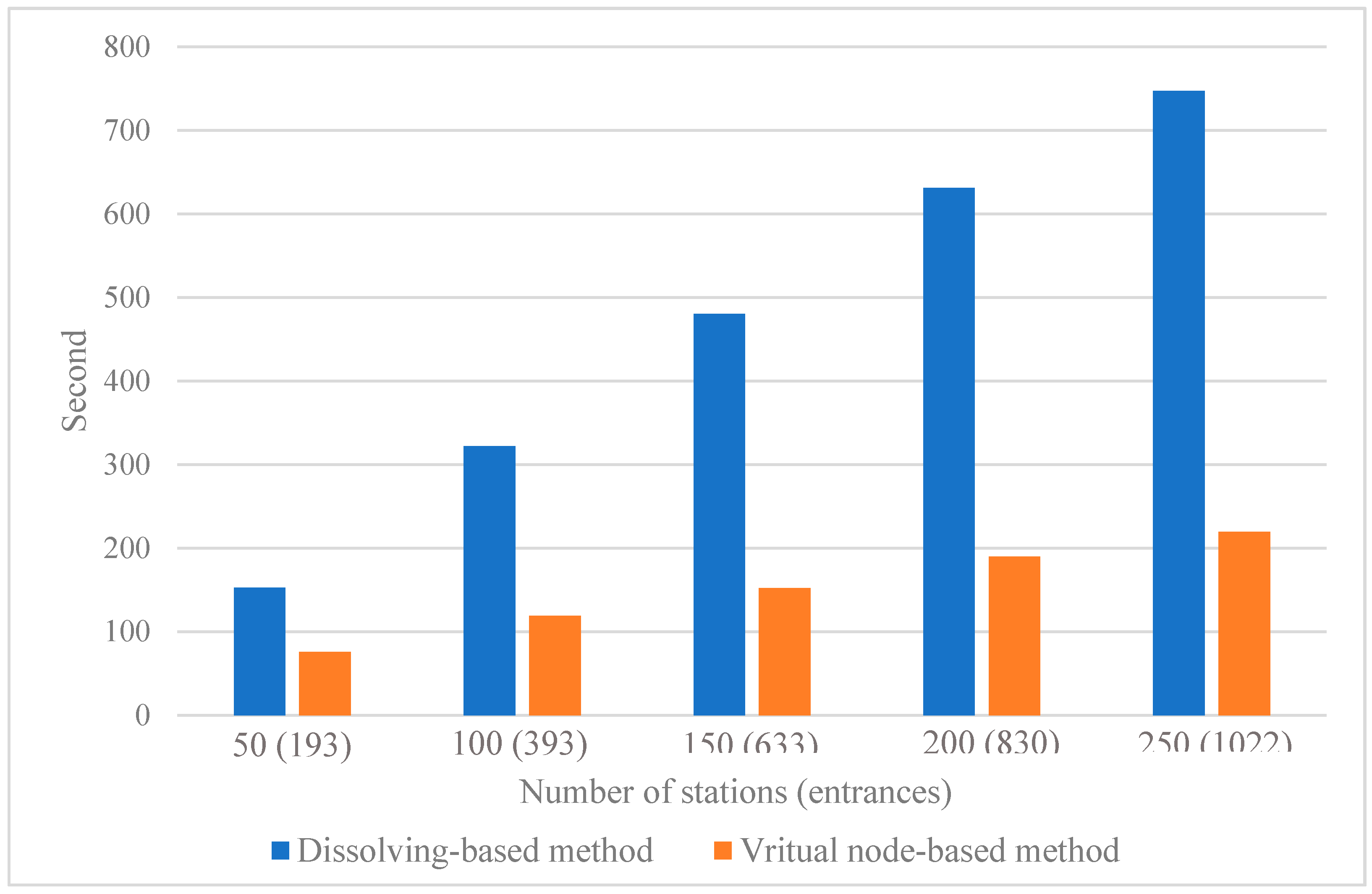
3.4.2. Non-Point Facility
In this experiment, we randomly select 5 different numbers of metro stations, i.e., 50, 100, 150, 200 and 250, to test the running time based on the dissolving-based and virtual node-based methods. The two methods are conducted using the proposed method and the cut-off distance is set to 1.2 km. For the dissolving-based method, the running time represents the time used for generating individual catchment areas of all the entrances, i.e., the time for dissolving the catchment areas is not included. Similar to experiment 1, the same experiment is conducted three times for each experimental setting, and the average running time is deemed to be the final running time. As shown by the results listed in Figure 13, we observe a sharp drop in the running time when the virtual node-based method is used for generating the metro catchment areas. Such a drop indicates that the virtual node-based method can largely improve the time efficiency, and the improvement is more obvious with the increase of the number of input facilities. Furthermore, no additional dissolving procedure is required by the virtual node-based method. Combined with the results obtained in Figure 12, we can infer that the virtual node-based method can achieve an even larger improvement in efficiency if the dissolving-based method is conducted using ArcGIS.
4. Discussion
The impedance of a network edge is measured by its length in this study. In practice, we may use travel time rather than length as the impedance. The proposed framework can be easily applied to generate the TCA within a given cut-off time through minor modifications. Specifically, the modification occurs at the step of subgraph construction, i.e., the cut-off time needs to be transferred to a cut-off distance to define the size of the searching box. Such a transfer can be achieved by multiplying the cut-off time by the maximum walking speed of road edges.
Furthermore, other potential environmental factors, such as road quality (e.g., road material) and connectivity, can be incorporated into the travel impedance modeling [40]. For instance, the sidewalk is an important element that may need consideration for defining the travel impedance of walking. In general, the impact of these elements can be modeled by incorporating additional weighing factors to the length of road edges. The updated travel impedance of an edge is denoted as follows.
where is the new impedance of, . is the length of, and is the weighting function determined by considered influence factors. Hence, a new weighted road network can be constructed and used to support the new approach for the generation of TCAs.
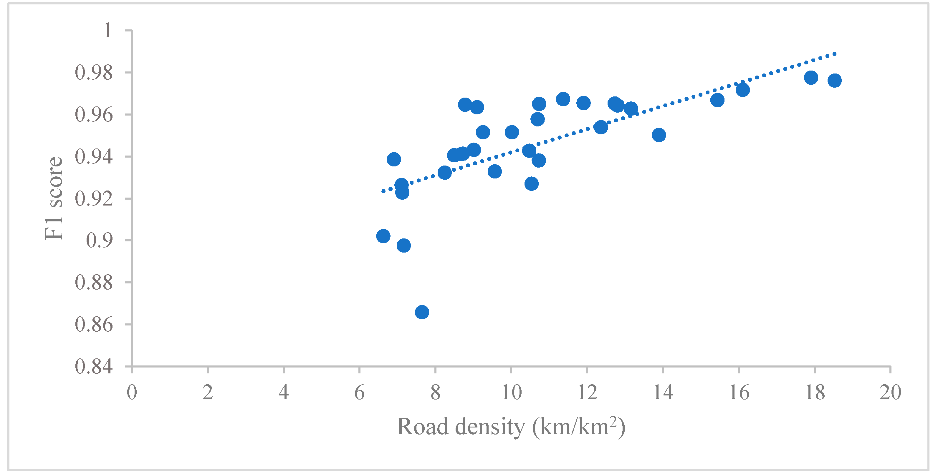
The interpolation based on the constrained Delaunay triangulation is one of the key components of the proposed framework. Since all road segments are included as the constraints during the triangulation, the interpolated distances along the network are thus guaranteed to be accurate. On the other hand, the interpolation by triangulation cannot guarantee an accurate result for the off-network area. This is reflected by the accuracy evaluation of generated TCAs (i.e., the precision and recall are both below 100%). Generally, the high F1 score indicates that such a triangulation-based method offers a reasonable accuracy of TCAs in the urban context. This can be partly explained by the high density of roads in urban areas because a high road density means more network nodes are involved during the interpolation. Figure 14 shows an example of the scatter plot between the road density and the F1 scores. The road density is measured as the ratio of the total length of subgraph edges to the area of the corresponding searching box. The F1 scores correspond to the evaluation of the 32 catchment areas generated by our method under the cut-off distance of 1.2 km (see Section 3.3.2). As shown, although it is not a linear relationship, the distribution generally indicates that a higher density of road is likely to have a better F1 score.
It is important to note the F1 score is an integrated accuracy evaluation from the geospatial perspective. A high F1 score means a high similarity of the generated catchment area and the real catchment area. In this way, such a metric is especially useful when the generated catchment area is employed to differentiate the transit-served areas from underserved areas. If the generated catchment area is specifically used for estimating the population being covered by a station (e.g., for transit ridership modeling), we may need additional metrics to evaluate the performance of a TCA generation method, i.e., metrics to test how the covered population estimated by the generated TCAs is different from the real covered population. For instance, a comparison of the total population of the accessible points and the covered population by the catchment area could be a possible approach.
As demonstrated by the time efficiency evaluation, the proposed framework is especially useful for a fast TCA generation of non-point transit facilities (e.g., rail transit stations). For instance, identifying a suitable cut-off distance for transit ridership modeling from a series of candidates (e.g., 600–1200 m) is a typical time-consuming scenario. The running time of our method is largely affected by the cut-off distance. A larger cut-off distance means a larger size of subgraph and more computing time for the construction of the extended SP tree and constrained Delaunay triangulation. For transit catchment areas by walking, the cut-off distances usually are small, which makes the running time can be limited at a reasonable level. In our test, we find that the most time-consuming part of the processing is the construction of constrained Delaunay triangulation. Therefore, reducing the number of constraint edges is a possible way to improve time efficiency. Correspondingly, a preprocess of road simplification (e.g., remove the intermediate points of a straight road edge) could help accelerate the generation of catchment areas.
5. Conclusions
Generating the network-based TCA is one of the prerequisites for TCA-related analysis. It is therefore highly desirable to make this service sharable and transparent to the public. The open-source method would be particularly useful for those who have limited access to commercial Geographic Information System (GIS) software and researchers who wish to develop more sophisticated models for catchment area generation (e.g., integrating more routing-related factors). Our open-source framework of generating TCAs by walking is developed for this purpose. The methodological framework includes three components of the process: subgraph constructions, extended SP tree construction, and contour generation. The methods on how to extend the framework to the directed graph and non-point facilities are developed. The implementation of the framework is provided as an open-source project. We illustrate the feasibility of our framework using metro stations in Shanghai as case studies and show the advantages of our methods by comparing with four alternative methods. We quantitatively evaluate the feasibility and effectiveness of the proposed methods. The results show that the precisions and the recalls of the generated TCAs are above 90% and the F1 scores are comparable with the ArcGIS method. The running time of the proposed method is much faster than the ArcGIS method under the nine different experimental settings. The proposed framework is especially efficient in generating a larger number of catchment areas of non-point facilities.
Future work of this study can be conducted in the following aspects. First, the catchment areas generated by the proposed framework can be overlapped with each other. It is worthwhile exploring how to generate a non-overlapped catchment area. For instance, similar to [24], Voronoi polygons can be used to cut the overlapped catchment areas to generate mutually exclusive catchment areas, where the major difficulty would be the generation of “network-based” Voronoi polygons. Alternatively, we can divide the overlapped areas into small grids [26] and assign each grid to its nearest facility to create the non-overlapped catchment areas. Second, the framework is designed for generating TCAs by walking. Applying the framework to generate TCAs by other transport modes is also possible but needs more in-depth study. For example, how to improve the computation time under a large cut-off distance (e.g., 10 km) is an interesting question. Finally, from the aspect of implementation, we plan to design a more user-friendly interface for our framework. For instance, implementing our methods as a QGIS plugin is an appealing option.
Author Contributions
Conceptualization, Diao Lin; Methodology, Diao Lin; Software, Diao Lin; Validation, Diao Lin; Formal Analysis, Diao Lin; Data Curation, Diao Lin; Writing-Original Draft Preparation, Diao Lin; Writing-Review & Editing, Ruoxin Zhu, Jian Yang and Liqiu Meng; Visualization, Diao Lin; Supervision, Liqiu Meng. All authors have read and agreed to the published version of the manuscript.
Funding
This research is supported by China’s National Key R&D Program (grant No.2017YFB0503500) and National Natural Science Foundation of China (grant No.41901335). The APC is funded by the German Research Foundation (DFG) and the Technical University of Munich (TUM) in the framework of the Open Access Publishing Program.
Conflicts of Interest
The authors declare no conflict of interest. The funders had no role in the design of the study; in the collection, analyses, or interpretation of data; in the writing of the manuscript; or in the decision to publish the results.
References
- Lin, T.G.; Xia, J.C.; Robinson, T.P.; Olaru, D.; Smith, B.; Taplin, J.; Cao, B. Enhanced Huff model for estimating Park and Ride (PnR) catchment areas in Perth, WA. J. Transp. Geogr. 2016, 54, 336–348. [Google Scholar] [CrossRef] [Green Version]
- Dolega, L.; Pavlis, M.; Singleton, A. Estimating attractiveness, hierarchy and catchment area extents for a national set of retail centre agglomerations. J. Retail. Consum. Serv. 2016, 28, 78–90. [Google Scholar] [CrossRef] [Green Version]
- Lieshout, R. Measuring the size of an airport’s catchment area. J. Transp. Geogr. 2012, 25, 27–34. [Google Scholar] [CrossRef]
- Kimpel, T.J.; Dueker, K.J.; El-Geneidy, A.M. Using GIS to Measure the Effect of Overlapping Service Areas on Passenger Boardings at Bus Stops. Urban Reg. Inf. Syst. Assoc. J. 2007, 19, 5–11. [Google Scholar]
- Gutiérrez, J.; García-Palomares, J.C. Distance-measure impacts on the calculation of transport service areas using GIS. Environ. Plan. B Plan. Des. 2008, 35, 480–503. [Google Scholar] [CrossRef]
- García-Palomares, J.C.; Sousa Ribeiro, J.; Gutiérrez, J.; Sá Marques, T. Analysing proximity to public transport: The role of street network design. Boletín Asoc. Geógrafos Españoles 2018, 102–130. [Google Scholar] [CrossRef] [Green Version]
- Riggs, W.; Chamberlain, F. The TOD and smart growth implications of the LA adaptive reuse ordinance. Sustain. Cities Soc. 2018, 38, 594–606. [Google Scholar] [CrossRef]
- Zacharias, J.; Zhao, Q. Local environmental factors in walking distance at metro stations. Public Transp. 2018, 10, 91–106. [Google Scholar] [CrossRef]
- Gutiérrez, J.; Cardozo, O.D.; García-Palomares, J.C. Transit ridership forecasting at station level: An approach based on distance-decay weighted regression. J. Transp. Geogr. 2011, 19, 1081–1092. [Google Scholar] [CrossRef]
- Lee, S.; Yi, C.; Hong, S.P. Urban structural hierarchy and the relationship between the ridership of the Seoul Metropolitan Subway and the land-use pattern of the station areas. Cities 2013, 35, 69–77. [Google Scholar] [CrossRef]
- Langford, M.; Fry, R.; Higgs, G. Measuring transit system accessibility using a modified two-step floating catchment technique. Int. J. Geogr. Inf. Sci. 2012, 26, 193–214. [Google Scholar] [CrossRef]
- El-Geneidy, A.; Grimsrud, M.; Wasfi, R.; Tétreault, P.; Surprenant-Legault, J. New evidence on walking distances to transit stops: Identifying redundancies and gaps using variable service areas. Transportation 2014, 41, 193–210. [Google Scholar] [CrossRef]
- Wang, Z.; Chen, F.; Xu, T. Interchange between Metro and Other Modes: Access Distance and Catchment Area. J. Urban Plan. Dev. 2016, 142, 04016012. [Google Scholar] [CrossRef]
- Páez, A.; Scott, D.M.; Morency, C. Measuring accessibility: Positive and normative implementations of various accessibility indicators. J. Transp. Geogr. 2012, 25, 141–153. [Google Scholar] [CrossRef]
- Hsiao, S.; Lu, J.; Sterling, J.; Weatherford, M. Use of geographic information system for analysis of transit pedestrian access. Transp. Res. Rec. 1997, 50–59. [Google Scholar] [CrossRef]
- O’Sullivan, S.; Morrall, J. Walking Distances to and from Light-Rail Transit Stations. Transp. Res. Rec. 1996, 1538, 19–26. [Google Scholar] [CrossRef]
- Zhao, J.; Deng, W. Relationship of Walk Access Distance to Rapid Rail Transit Stations with Personal Characteristics and Station Context. J. Urban Plan. Dev. 2013, 139, 311–321. [Google Scholar] [CrossRef]
- Jun, M.J.; Choi, K.; Jeong, J.E.; Kwon, K.H.; Kim, H.J. Land use characteristics of subway catchment areas and their influence on subway ridership in Seoul. J. Transp. Geogr. 2015, 48, 30–40. [Google Scholar] [CrossRef]
- Macias, K. Alternative methods for the calculation of pedestrian catchment areas for public transit. Transp. Res. Rec. 2016, 2540, 138–144. [Google Scholar] [CrossRef]
- Xi, Y.; Saxe, S.; Miller, E. Accessing the subway in Toronto, Canada: Access mode and catchment areas. Transp. Res. Rec. 2016, 2543, 52–61. [Google Scholar] [CrossRef]
- Bhat, C.; Bricka, S.; La Mondia, J.; Kapur, A.; Guo, J.; Sen, S. Metropolitan Area Transit Accessibility Analysis Tool; No. Report No. 0-5178-P3; Public Transportation Service: Austin, TX, USA, 2006. [Google Scholar]
- Foda, M.; Osman, A. Using GIS for Measuring Transit Stop Accessibility Considering Actual Pedestrian Road Network. J. Public Transp. 2010, 13, 23–40. [Google Scholar] [CrossRef] [Green Version]
- Young, M. Defining probability-based rail station catchments for demand modelling. In Proceedings of the 48th Annual UTSG Conference, Bristol, UK, 6–8 January 2016; pp. 1–12. [Google Scholar]
- Haggett, P.; Cliff, A.D.; Frey, A. Locational Analysis in Human Geography, 1st ed.; Edward Arnold: London, UK, 1977. [Google Scholar]
- Delamater, P.L.; Messina, J.P.; Shortridge, A.M.; Grady, S.C. Measuring geographic access to health care. Int. J. Health Geogr. 2012, 11, 15. [Google Scholar] [CrossRef] [PubMed] [Green Version]
- Upchurch, C.; Kuby, M.; Zoldak, M.; Barranda, A. Using GIS to generate mutually exclusive service areas linking travel on and off a network. J. Transp. Geogr. 2004, 12, 23–33. [Google Scholar] [CrossRef]
- Lin, D.; Zhang, Y.; Zhu, R.; Meng, L. The analysis of catchment areas of metro stations using trajectory data generated by dockless shared bikes. Sustain. Cities Soc. 2019, 101598. [Google Scholar] [CrossRef]
- Service Area Analysis—Help|Documentation. Available online: https://desktop.arcgis.com/en/arcmap/latest/extensions/network-analyst/service-area.htm (accessed on 18 June 2020).
- Edler, D.; Husar, A.; Keil, J.; Vetter, M.; Dickmann, F. Virtual reality (VR) and open source software: A workflow for constructing an interactive cartographic VR environment to explore urban landscapes. Kartogr. Nachr. 2018, 5–13. [Google Scholar] [CrossRef]
- Garnett, R.; Kanaroglou, P. Qualitative GIS: An open framework using spatialite and open source GIS. Trans. GIS 2016, 20, 144–159. [Google Scholar] [CrossRef]
- Coetzee, S.; Ivánová, I.; Mitasova, H.; Brovelli, M.A. Open geospatial software and data: A review of the current state and a perspective into the future. ISPRS Int. J. GeoInf. 2020, 9, 90. [Google Scholar] [CrossRef] [Green Version]
- Guttman, A. R-trees: A dynamic index structure for spatial searching. In Proceedings of the 1984 ACM SIGMOD International Conference on Management of Data—SIGMOD, New York, NY, USA, 1 June 1984; ACM Press: New York, NY, USA, 1984. [Google Scholar] [CrossRef]
- Roussopoulos, N.; Kelley, S.; Vincent, F. Nearest neighbor queries. In Proceedings of the ACM SIGMOD international conference on Management of data, San Jose, CA, USA, 22 May 1995; Michael, C., Donovan, S., Eds.; Association for Computing Machinery: New York, NY, USA, 1995; pp. 71–79. [Google Scholar] [CrossRef]
- Yang, C.; Gidófalvi, G. Fast map matching, an algorithm integrating hidden Markov model with precomputation. Int. J. Geogr. Inf. Sci. 2018, 32, 547–570. [Google Scholar] [CrossRef]
- Okabe, A.; Okunuki, K.I.; Shiode, S. The SANET toolbox: New methods for network spatial analysis. Trans. GIS 2006, 10, 535–550. [Google Scholar] [CrossRef]
- Okabe, A.; Sugihara, K. Spatial Analysis along Networks: Statistical and Computational Methods, 1st ed.; Wiley: New Jersey, NJ, USA, 2012. [Google Scholar]
- Boissonnat, J.; Devillers, O.; Pion, S.; Teillaud, M.; Boissonnat, J.; Devillers, O.; Pion, S.; Teillaud, M.; Yvinec, M.; Boissonnat, J. Triangulations in CGAL. Comput. Geom. 2007, 22, 5–19. [Google Scholar] [CrossRef] [Green Version]
- Watson, D. Contouring: A Guide to the Analysis and Display of Spatial Data, 1st ed.; Pergamon: Oxford, UK, 1992. [Google Scholar]
- Boeing, G. OSMnx: New methods for acquiring, constructing, analyzing, and visualizing complex street networks. Comput. Environ. Urban Syst. 2017, 65, 126–139. [Google Scholar] [CrossRef] [Green Version]
- Van Soest, D.; Tight, M.R.; Rogers, C.D.F. Exploring the distances people walk to access public transport. Transp. Rev. 2020, 40, 160–182. [Google Scholar] [CrossRef]
Figure 1.
Framework of generating the network-based transit catchment areas by walking.

Figure 2.
Example of subgraph construction of a facility.

Figure 3.
Demonstration of an extended shortest path tree.

Figure 4.
Algorithm of finding the non-SP tree edges of a facility.

Figure 5.
Illustration of the interpolations based on the shortest (a) and extended shortest path trees (b).
Figure 5.
Illustration of the interpolations based on the shortest (a) and extended shortest path trees (b).

Figure 6.
Illustration of the interpolations based on the Delaunay and constrained Delaunay triangulations.
Figure 6.
Illustration of the interpolations based on the Delaunay and constrained Delaunay triangulations.

Figure 7.
Illustration of accessible and inaccessible points within the searching box.

Figure 8.
The process of catchment area generation of a point facility based on an undirected road network. (a) sub-edges; (b) shortest path (SP) tree and non-SP tree edges; (c) constrained Delaunay triangulation; (d) accessible edges and catchment area.
Figure 8.
The process of catchment area generation of a point facility based on an undirected road network. (a) sub-edges; (b) shortest path (SP) tree and non-SP tree edges; (c) constrained Delaunay triangulation; (d) accessible edges and catchment area.

Figure 9.
The from-facility (a) and to-facility (b) catchment area of a point facility based on a directed road network.
Figure 9.
The from-facility (a) and to-facility (b) catchment area of a point facility based on a directed road network.
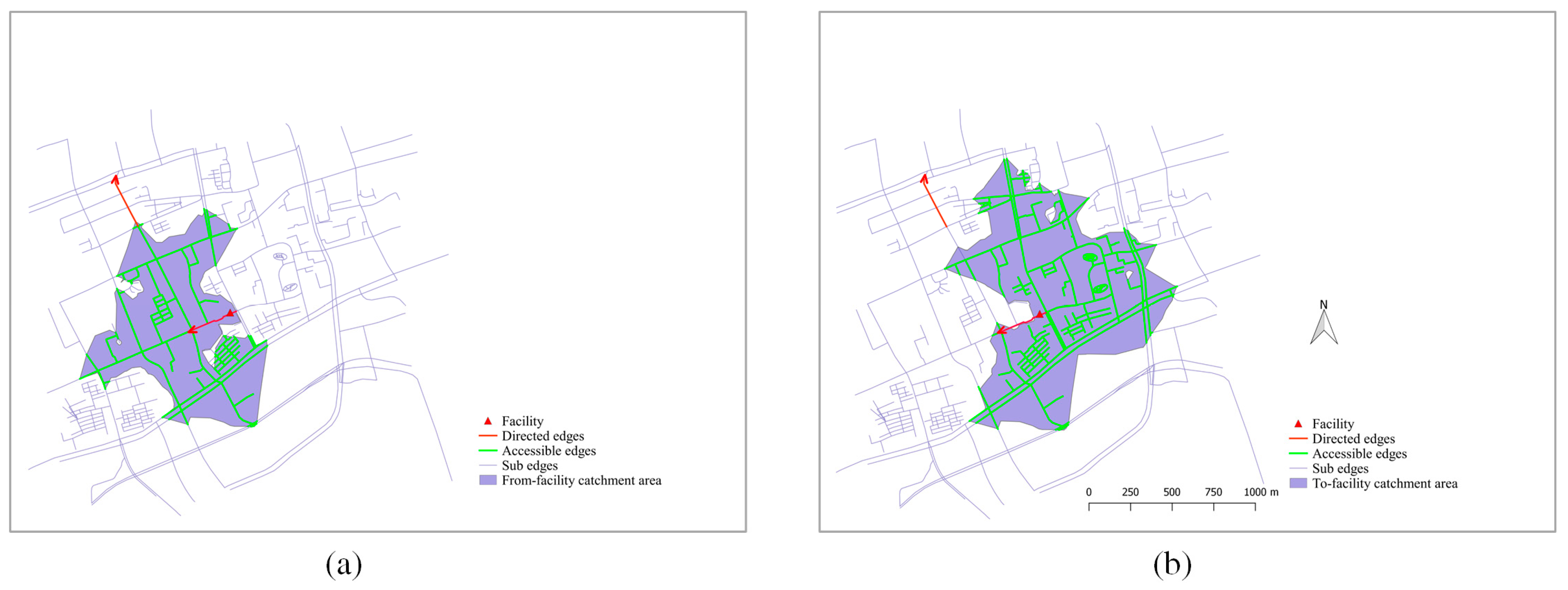
Figure 10.
The catchment area of a multiple-point facility based on an undirected road network.
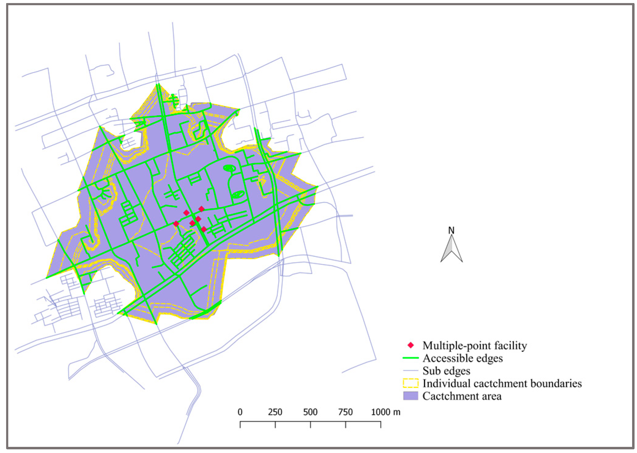
Figure 11.
The catchment areas generated by five different methods.

Figure 12.
Running times of the ArcGIS method and our method under nine different experimental settings.
Figure 12.
Running times of the ArcGIS method and our method under nine different experimental settings.
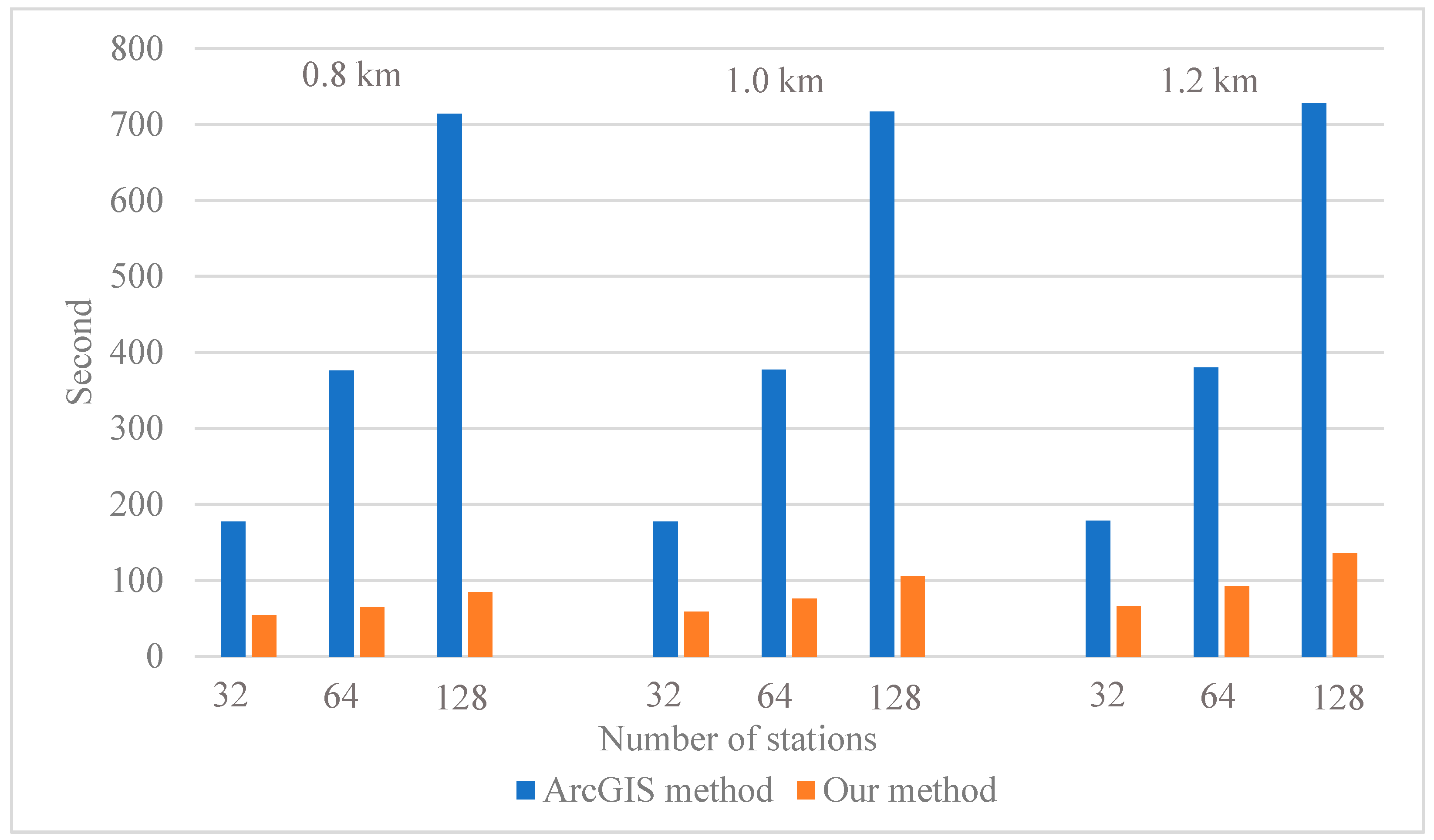
Figure 13.
Running times of generating the catchment areas of non-point facilities using the virtual node-based and dissolving-based methods. Both methods are conducted via the proposed method and the cut-off distance is 1.2 km for all the experimental settings.
Figure 13.
Running times of generating the catchment areas of non-point facilities using the virtual node-based and dissolving-based methods. Both methods are conducted via the proposed method and the cut-off distance is 1.2 km for all the experimental settings.

Figure 14.
Relationship between road densities and F1 scores. The F1 scores correspond to the evaluation of the 32 catchment areas generated by our framework under the cut-off distance of 1.2 km.
Figure 14.
Relationship between road densities and F1 scores. The F1 scores correspond to the evaluation of the 32 catchment areas generated by our framework under the cut-off distance of 1.2 km.


Table 1.
The statistics for 32 stations under different cut-off distances.
| Cut-off Distance (km) | Average Number of Grid Points in the TCAs | Average Precision | Average Recall | Average F1 Score | ||||
|---|---|---|---|---|---|---|---|---|
| ArcGIS | Ours | ArcGIS | Ours | ArcGIS | Ours | ArcGIS | Ours | |
| 0.8 | 9271 | 10217 | 0.932 | 0.908 | 0.885 | 0.954 | 0.904 | 0.928 |
| 1.0 | 15120 | 16798 | 0.948 | 0.916 | 0.891 | 0.962 | 0.914 | 0.937 |
| 1.2 | 22480 | 25049 | 0.955 | 0.921 | 0.899 | 0.973 | 0.924 | 0.946 |
© 2020 by the authors. Licensee MDPI, Basel, Switzerland. This article is an open access article distributed under the terms and conditions of the Creative Commons Attribution (CC BY) license (http://creativecommons.org/licenses/by/4.0/).
Share and Cite
MDPI and ACS Style
Lin, D.; Zhu, R.; Yang, J.; Meng, L. An Open-Source Framework of Generating Network-Based Transit Catchment Areas by Walking. ISPRS Int. J. Geo-Inf. 2020, 9, 467. https://0-doi-org.brum.beds.ac.uk/10.3390/ijgi9080467
AMA Style
Lin D, Zhu R, Yang J, Meng L. An Open-Source Framework of Generating Network-Based Transit Catchment Areas by Walking. ISPRS International Journal of Geo-Information. 2020; 9(8):467. https://0-doi-org.brum.beds.ac.uk/10.3390/ijgi9080467
Chicago/Turabian StyleLin, Diao, Ruoxin Zhu, Jian Yang, and Liqiu Meng. 2020. "An Open-Source Framework of Generating Network-Based Transit Catchment Areas by Walking" ISPRS International Journal of Geo-Information 9, no. 8: 467. https://0-doi-org.brum.beds.ac.uk/10.3390/ijgi9080467
Note that from the first issue of 2016, this journal uses article numbers instead of page numbers. See further details here.