Spatio-Temporal Visualization Method for Urban Waterlogging Warning Based on Dynamic Grading

Abstract

With the acceleration of the urbanization process, the problems caused by extreme weather such as heavy rainstorm events have become more and more serious. During such events, the road and its auxiliary facilities may be damaged in the process of the rainstorm and waterlogging, resulting in the decline of its traffic capacity. Rainfall is a continuous process in a space–time dimension, and as rainfall data are obtained through discrete monitoring stations, the acquired rainfall data have discrete characteristics of time interval and space. In order to facilitate users in understanding the impact of urban waterlogging on traffic, the visualization of waterlogging information needs to be displayed under different spatial and temporal granularity. Therefore, the appropriateness of the visualization granularity directly affects the user’s cognition of the road waterlogging map. To solve this problem, this paper established a spatial granularity and temporal granularity computing quantitative model for spatio-temporal visualization of road waterlogging and the evaluation method of the model was based on the cognition experiment. The minimum visualization unit of the road section is 50 m and we proposed a 5-level depth grading method and two color schemes for road waterlogging visualization based on the user’s cognition. To verify the feasibility of the method, we developed a prototype system and implemented a dynamic spatio-temporal visualization of the waterlogging process in the main urban area of Nanjing, China. The user cognition experiment showed that most participants thought that the segmentation of road was helpful to the local visual expression of waterlogging, and the color schemes of waterlogging depth were also helpful to display the road waterlogging information more effectively.

1. Introduction

Flood disaster is the most common meteorological disaster. According to statistics, the loss caused by flood disaster alone is as high as 40% every year worldwide. Against the background of rapid urbanization, with new construction, reconstruction, and expansion projects changing the original surface conditions and increasing the impervious area, the problem of urban waterlogging has become more and more serious [1,2]. The rainstorm and waterlogging disaster will affect many aspects of the complex system of the city, for example, the road and its ancillary facilities will be damaged in the process of the rainstorm and waterlogging, resulting in the decline of its traffic capacity; once the traffic system is interrupted or paralyzed, it will have a very adverse impact on the production and life of the city. Among them, the urban transportation system, as the skeleton of the city and the carrier of travel, is the most vulnerable bearing body in rainstorms and waterlogging [3]. In disaster management, an accurate focal priority analysis of how societies can adapt to these changing events can provide insight into practical solutions [4]. Therefore, we can improve the pertinence and effectiveness of meteorological service, and bring the benefits of meteorological service into full play to carry out an early warning service of urban waterlogging.

For first-tier cities, through meteorological stations, hydrological observation stations, and road water sensors throughout the city, a large number of continuous and various forms of meteorological monitoring data will be generated every day. With the help of these meteorological data, and through the integration with the terrain, road network, road condition, and VGI (volunteer geographic information) data, a large spatio-temporal dataset can be used by the meteorological department to monitor and forecast urban waterlogging, and effectively assist the relevant departments to evaluate the waterlogging of the road.

Road waterlogging decreases driving safety [5]. At present, most of the visualization of urban waterlogging is to show the area and depth of waterlogging. However, two issues should be discussed if these maps want to show the impact of traffic. First, the urban waterlogging situation is generally grid surface data when visualized, but the road and its traffic conditions are mostly vector line data. The difference between the two types of data brings difficulties to the comprehensive assessment of road conditions, so it is necessary to match. Second, due to the interconnectivity of the road network, the impact of traffic flow and water depth on the road conditions are not global, only affecting the corresponding waterlogging road sections, therefore, the granularity of road sections in different scales needs to be selected appropriately.

However, due to the gaps in different professional fields, there is no effective method of dynamic grading for visualization to show the depth of road waterlogging, and the public cannot understand this information in an intuitive form, resulting in its prediction failing to give fully understanding. It is an important step to classify the complicated geographical phenomena to different levels to improve the map availability. Due to the spatial heterogeneity of urban waterlogging and the complexity of its geographical process, dynamic grading in the visualization process must be considered when visualizing the depth of road waterlogging in different level. For the geometric and semantic features of the road such as the depth of waterlogging, traffic flow, and road surface flatness, which are often expressed in linear form, they have the attributes of spatial heterogeneity. In the process of visualization, the road is usually divided into several small sections with a certain length to realize its spatial distribution. Due to the spatio-temporal changing characteristics of urban waterlogging, it is still lack of methods which are suitable for the dynamic grading of road waterlogging dynamiclly.

This paper aimed at the visualization of waterlogging information displayed under different spatial and temporal granularity. The situation of road waterlogging often occurs in local road sections, so it needs multi-scale and multi-level expression based on the road sections in the spatio-temporal visualization. The visualization of road waterlogging in spatio-temporal animation provides a scientific reference for the disaster prevention department and the traffic management department to specify emergency strategies, help the public understand the road conditions of accumulated waterlogging information, and is beneficial in adjusting their travel plans.

2. Related Work

2.1. Road Waterlogging: Definitions and Evaluation Metrics

Urban waterlogging refers to the phenomenon that heavy rainfall or continuous rainfall in urban areas exceeds the capacity of urban rainwater facilities, causing waterlogging in urban areas [6]. Extreme precipitation events and the resulting urban rainstorms were first found in developed countries in Europe and America which had rapid urbanization, and then caused worldwide attention [7,8,9]. The occurrence of urban waterlogging is mainly caused by the following four reasons [10]: (1) Extreme heavy rain events; (2) Waterlogging in the outer river; (3) Changes in the underlying surface of the city affect the law of production and confluence; and (4) The planning and design of drainage systems are unreasonable.

Road waterlogging in urban environments is mainly due to the road surface elevation being lower than that of the surrounding surfaces (especially concave overpasses), and the water permeability of the hardened ground is reduced, so the precipitation caused by heavy rain cannot be discharged through surface runoff or discharged through infiltration, so has to gather on the road surface.

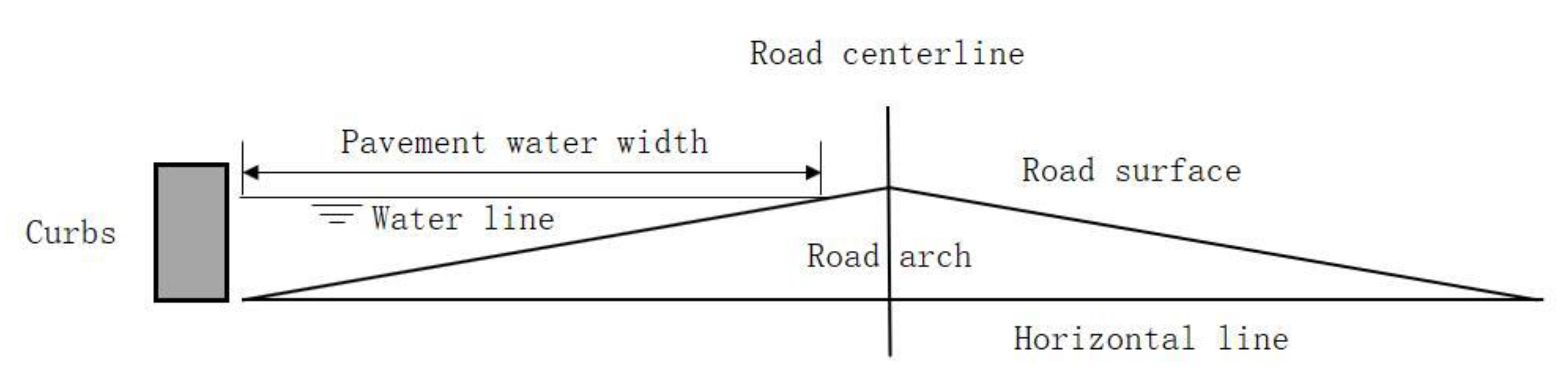
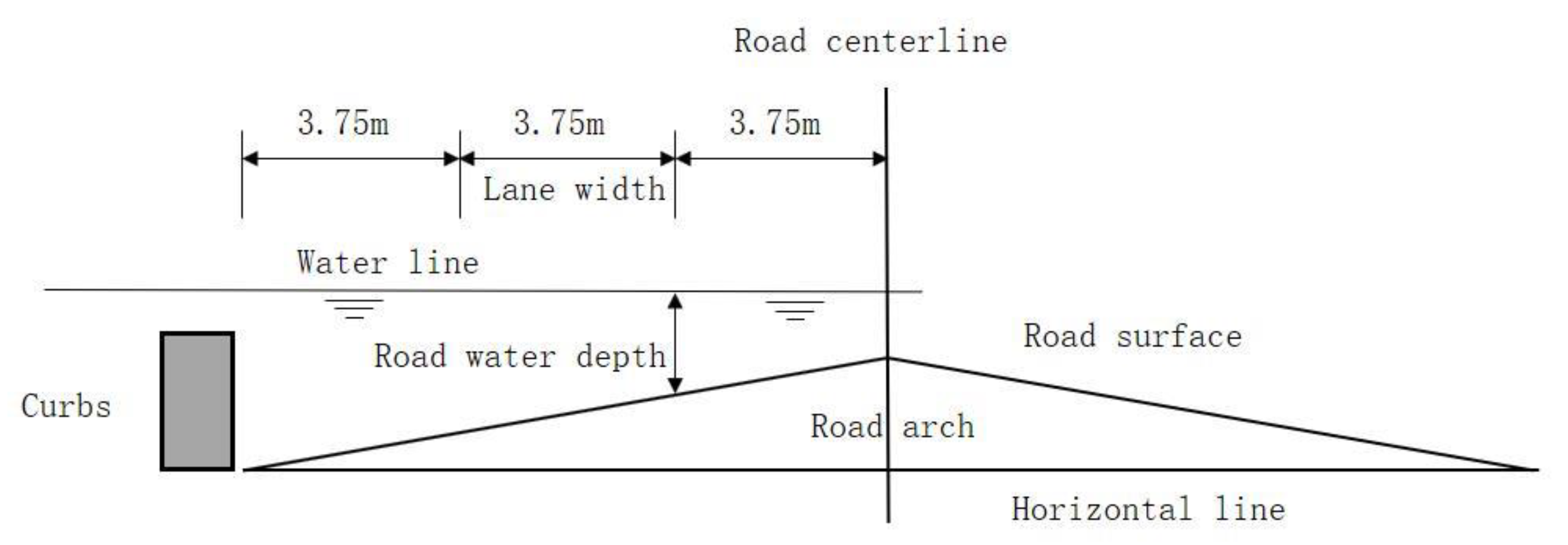
Road waterlogging is usually measured by two indexes: (1) width of road pavement water; and (2) depth of road water [6]. The width of the road pavement water refers to the width of the water in the direction of the road curbs to the road centerline (Figure 1), the depth of the road water is the deepest water depth on the lane; when there are multiple lanes on each side of the road’s centerline, then the lane closest to the road arch is measured (Figure 2). Therefore, it should be noted that during the measuring process, the former does not need to consider the number and width of lanes, while the latter is the opposite.

2.2. Data Acquisition and Simulation of Urban Waterlogging

Ideally, urban waterlogging data should be monitored by waterlogging sensors, however, the current monitoring data of waterlogging sensors cannot reflect the spatio-temporal distribution characteristics of urban waterlogging. Scholars widely use hydrological and rain waterlogging models to simulate and calculate waterlogging under different rainfall scenarios, in order to evaluate and predict the spatio-temporal distribution of waterlogging [11,12].

However, the rain waterlogging models are more concerned with the calculation process of waterlogging simulations. From the perspective of geographical visualization, to analyze and visualize the spatio-temporal process of urban waterlogging, it is necessary to study the construction of the urban waterlogging data model under the space–time dimension. The spatio-temporal data model is a data model for the centralized management of spatio-temporal data, where a significant feature is that the characteristic expression of spatio-temporal data is more complete than the traditional spatial data model, which solves the problem of limited type and quantity of spatio-temporal information [13,14]. The spatio-temporal data model has undergone rapid development since Langran and Chrisman [15] proposed spatiotemporal GIS (Geographic Information System), at this stage, there are four classic data models: the sequence snapshot model [16], ground state correction model [17], space–time composite model, and space–time cube model. On this basis, many scholars of geographic information science have proposed spatio-temporal data models for different application fields such as object-oriented data models [18], the event-based spatio-temporal data model (ESTDM) [19], etc. This greatly enriches the theory and application of the spatio-temporal data model. The spatio-temporal data model is a data model used to describe the spatio-temporal change process of geographical phenomena. At present, the study of spatio-temporal processes such as urban waterlogging is based on the spatio-temporal data model [20,21]. For the visual needs of road waterlogging, it is necessary to establish a spatio-temporal data model of road waterlogging.

2.3. Spatio-Temporal Visualization Methods

Spatio-temporal data models introduce the concept of granularity in storage, where a continuous entity is divided into multiple sets of discrete data with a similar size in the storage model in an orderly manner, and the granularity is the smallest unit. As the three dimensions of spatio-temporal data are space, time, and semantics, the granularity is also divided into spatial granularity, temporal granularity, and semantic granularity.

The research in this paper involves spatial granularity and temporal granularity. The spatial granularity of geo-information expresses the degree of detail of geographic information in the spatial scale, and it is most closely related to the level of geographic detail [22]. For spatial granularity, the interval is the direct distance of the sampling point, where the smaller the interval, the finer the space granularity. The size of the spatial granularity can be regarded as a split method of spatial data in the actual visual process. Zuo [23] once applied the method of dynamic segmentation to the management of road data, and commercial software Mapbox proposes the use of Vector Tiles to realize the spatial partition of vector data (Mapbox 2016) [24]. According to the constraints of scale and graphical constraints at the multi-scale visualization process, Wan [25] proposed a waterlogging rule between the granularity of riding trajectory division and the scaling level of a map.

On the other hand, temporal granularity refers to the frequency or time interval when an event or phenomenon occurs, and it is closely related to spatial granularity. Temporal granularity research in the spatio-temporal visualization usually directly depends on the sampling interval of the data itself [26]. In the visualization of the time dimension, more scholars have focused on the determination of time scale and the generation of frames based on time series [27]. Furthermore, if the events are visualized by animation, the duration and change rate of the visual symbol is also a temporal granularity [28].

3. Methodology

3.1. Extraction of Road Waterlogging Depth

The road waterlogging data obtained in this paper were provided by the Huaihe River Rainstorm and Waterlogging Early Warning System developed by the Jiangsu Meteorological Service Center, and the output result is the surface raster data [29]. In the process of spatio-temporal visualization of road waterlogging, the accuracy of the waterlogging depth extraction will directly affect the visualization effect. Therefore, the extraction of the waterlogging depth information from the obtained road waterlogging data involves two key issues: (1) how to match the raster road waterlogging data to the vector road network; and (2) how to correct the waterlogging depth change caused by the elevation of the road.

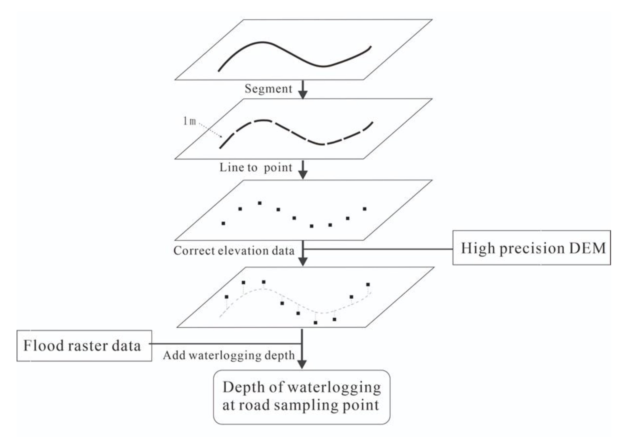
Therefore, in this paper, the following solutions are proposed. In the raster-format surface data returned by the simulation system, the value of each pixel indicates the average water depth based on the average elevation of the space in which the pixel is located. Since water is a fluid, we assumed that the water surface is flat, therefore, it is only necessary to know the actual elevation of the sampling point and offset it with the average elevation. Based on the solution of the above two issues, we proposed the following method for obtaining the depth of road water, and the main flow is shown in Figure 3.

This method is mainly divided into four stages: (1) Segment the road with a certain length, referring to the highest accuracy in the data source, and we set this length as 1 m; (2) Take the center point of the small section after splitting as the “Sampling point” of this section; (3) Calculate the deviation between the sampling point elevation and the average elevation of the pixel through high-precision DEM (Digital Elevation Model) data, deposit the data field “offset”; (4) Extract the depth information of the pixel where the sampling point is located and use the “offset” field to correct the depth of waterlogging and deposit it into the data field “Depth”. For the above steps, (1) to (3) are single operation, where the calculation result can be stored as intermediate data in the database for subsequent reuse, and (4) will execute once after each urban waterlogging calculation. Through this method, high-resolution waterlogging information can be obtained in various parts of the road network, and serves in the subsequent granularity study to calculate the water depth of road sub-sections under different granularity.

3.2. Grading of Road Waterlogging Depth and Color Design

In the “Technical guide for urban intrinsic risk warning service” [30], to accurately reflect the impact of urban waterlogging disasters on different disaster-bearing bodies, the editor divides urban waterlogging into four levels, and different depth division criteria are set according to different bearer bodies. The depth of road water affects the driving condition of vehicles, where we referred to the classification of waterlogging depth criteria. At the same time, in the map design, the visual variables should guarantee covering all entire range of values, so the level of 0–5 cm should be added. Furthermore, considering the consistency of numbers and that it is consistent with the change direction of the water depth, the reverse re-compilation level forms the visual variable level in the visualization system, as shown in

Table 1. Grading of water depth.

Level	Water Depth	Grade Meaning
0	0–5 cm	Basically nothing different
1	5–20 cm	Vehicle speed slowdown
2	20–55 cm	A few cars cannot pass
3	55–100 cm	Most cars cannot pass
4	>100 cm	Traffic is completely paralyzed

.

In the spatio-temporal visualization of road waterlogging, colors are used to show different levels of road water depth. The water depth color schemes of this paper are shown in

Table 2. Color design for water depth.

Water Depth	Color
	Scheme 1	Scheme 2
0–5 cm	RGB (44,212,53)	RGB (199,230,242)
5–20 cm	RGB (48,102,255)	RGB (84,197,237)
20–55 cm	RGB (255,255,0)	RGB (37,138,206)
55–100 cm	RGB (254,154,0)	RGB (0,61,135)
>100 cm	RGB (218,41,37)	RGB (0,7,68)

. Considering that the color setting needs to conform to the industry habits, Scheme 1 under similar color matching is given, where the tone changes from cold to warm, and the depth of waterlogging is smaller than that of green, which will give people a safer visual association, representing that the waterlogging situation at this time will not cause too much impact, and with the increase in the level, the color moves gradually to red, giving people a relatively tense visual feeling, which means that the level of road waterlogging at this time needs to be given attention. Furthermore, scheme 2 refers to Wu [31] for the relevant research results of waterlogging symbol design, where color design was carried out under a unified tone to show the depth of waterlogging, as in the user’s cognitive habits, the color blue can easily form an association with water, and the darker the color forms a psychological hint of increasing quantity.

3.3. Minimum Visualization Unit of Road Waterlogging

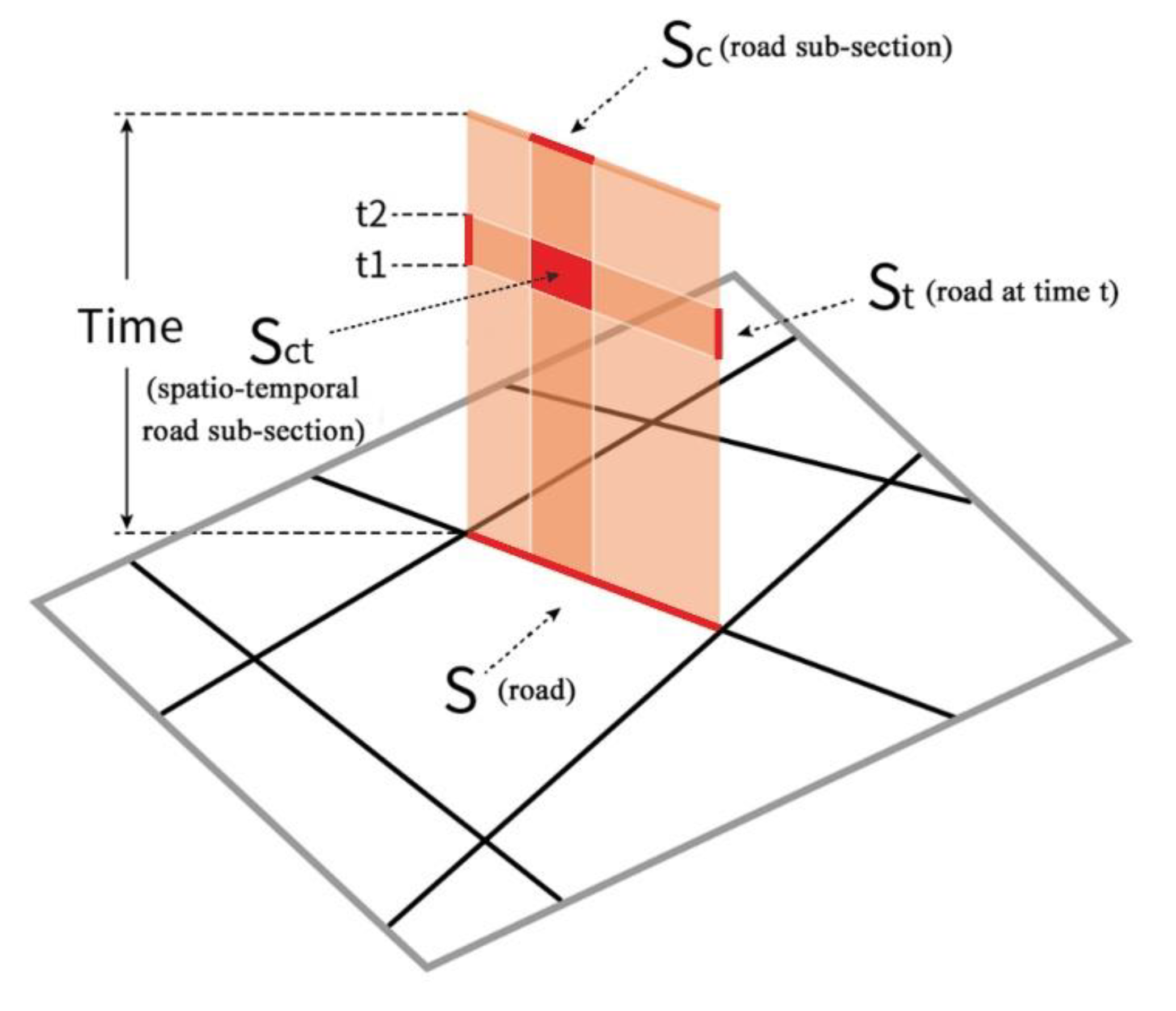
In spatio-temporal visualization, data can be divided into three levels: feature layer, target layer, and geometric detail layer [32]. The feature layer is the collection of the same kind of objects with the same semantics, and the feature refers to the waterlogging information of the road in this article. The target layer is an individual spatial feature with independent significance, and the target refers to the waterlogging depth of a single road in this article. The geometric detail layer is a structure divided by a single feature, and it is the basic unit of the target. For the spatio-temporal visualization of road waterlogging, we used “spatio-temporal road section” [33] as the smallest unit of visualization.

Due to the whole process of urban waterlogging, the depth of waterlogging in the road section will continue to change at different times. For example, in low-intensity continuous heavy rain, the waterlogging in the road section will gradually deepen when there is a single peak rain type, and the water depth on the road will show a trend of rising first and then falling with the change in rainfall. Therefore, for the road section, based on spatial visualization, the importance of the temporal dimension should also be considered. The temporal sub-section is the road between the two adjacent intersections in a certain period. As shown in Figure 4, based on section S, the timeline of the whole waterlogging process is added, a two-dimensional temporal sub-section is formed, and the time scale can include time measurement units such as year, month, day, hour, etc. Since road waterlogging is usually a manifestation of urban waterlogging caused by heavy rain, it shows the characteristic of non-periodic independent occurrence. Therefore, the time scale range of this paper is the process duration of single road waterlogging, St represents the section S of a certain period, and in the figure, it is the section S of the t1 to t2 period.

By combining the above two dimensions, a spatio-temporal road sub-section is generated. Based on the spatial distribution, section S is divided into multiple sub-sections Sc. Based on the time process of geographical process evolution, section S is divided into multiple sub-sections St; after the division of two dimensions, each two-dimensional segmentation unit is formed in the spatio-temporal road sub-section Sct, and each one constitutes the smallest unit of the spatio-temporal visualization of road waterlogging in this paper.

3.4. Construction of Spatio-Temporal Visual Granularity Model

The research of the granularity of space–time visualization, in the context of this paper, was to study how to divide the spatio-temporal road sub-section. The change of scale will cause changes in the expression environment of road waterlogging. Indeed, the spatial and temporal visualization granularity is the result of multiple influencing factors. In this process, the expansion of each factor will involve many specific problems. When building the spatial and temporal visual granularity calculation model for road waterlogging, it is necessary to analyze each cause of constraint that will eventually have an impact on spatial granularity and temporal granularity, respectively, as shown in

Table 3. Constraints on the visual granularity by different factors.

Constraint Factor	Spatial Granularity	Temporal Granularity
Characteristics of urban waterlogging	Sub-section upper limit	Time range upper limit
Multi-source data type and accuracy	Sub-section lower limit	Interval lower limit
Spatio-temporal visualization theory	Sub-section lower limit	Rate of change and total duration

.

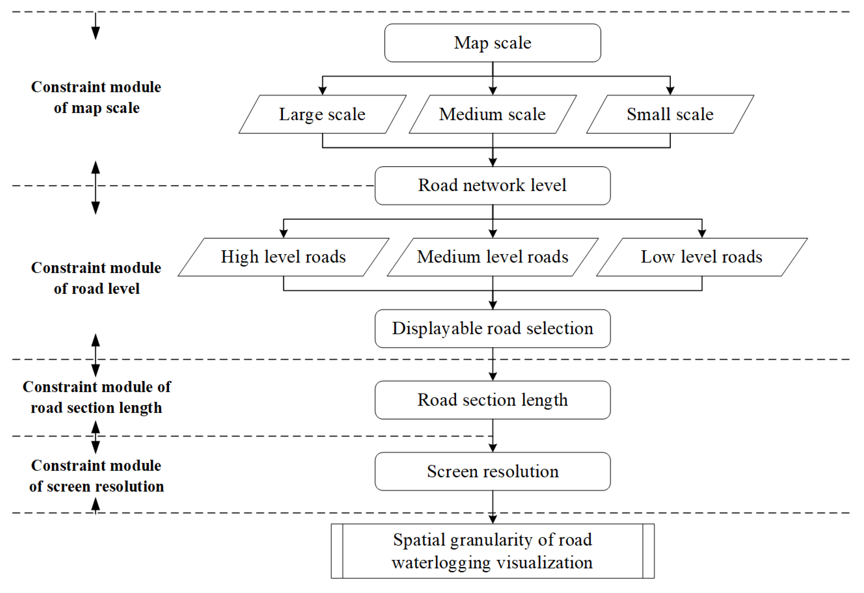
3.4.1. Spatial Granularity Calculation Model

The spatial granularity calculation model is shown in Figure 5, which is mainly divided into the following four modules. (1) Scale constraint module. This module limits the load quantity of road sections under the current scale, and the displayed road grades will change with the change of scale, that is, a dynamic constraint process is formed for the road network levels, thus indirectly constrains the expression of waterlogging information of road sections. (2) Road network hierarchy constraint module. The road network hierarchy constraint module restricts the specific sections and mesh that can carry waterlogging information and limits the base of spatial granularity through the selection of visible road. (3) Road section constraint module. At the current scale, the actual length of each section restricts the upper spatial granularity in the section. (4) Screen resolution constraint module. Screen resolution restricts the minimal division of spatial granularity.

3.4.2. Temporal Granularity Calculation Model

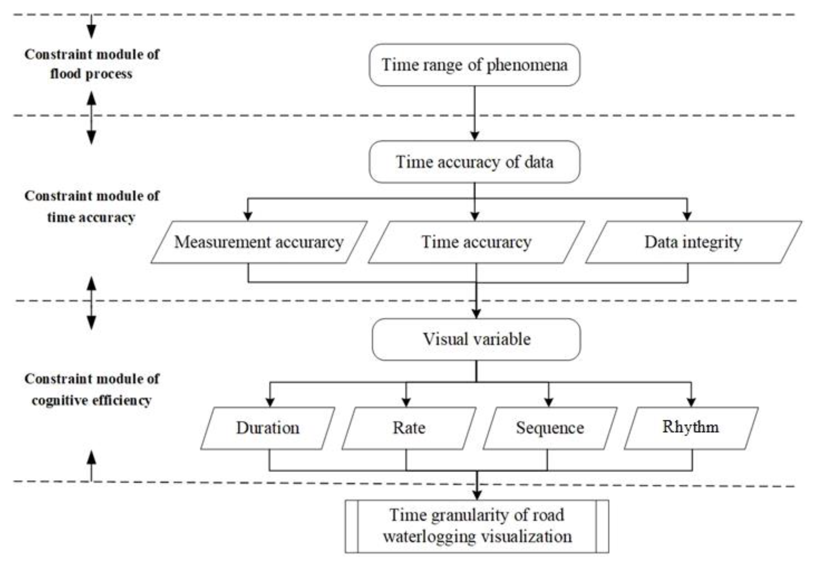
The temporal granularity calculation model is shown in Figure 6, which is mainly divided into the following three modules: (1) Waterlogging process constraint module. The module limits the upper limit of the range when the visualization schedule occurs, and the total duration of the waterlogging occurrence is the total duration of road waterlogging, and it is meaningless to divide the time granularity larger than the long interval at this time. (2) Time precision constraint module. The precision module of spatio-temporal data restricts the accuracy and practicality of space information, which is mainly affected by factors such as time measurement accuracy, time consistency, and time integrity, and the time accuracy of the data will directly affect the accuracy of the visual results. (3) Cognitive efficiency constraint module. Cognitive efficiency limits the lower limit of the minimum segmentation of time granularity. Affected by human cognitive efficiency, dynamic visual variables such as time duration, change rate, change order, and change rhythm should be fully utilized in the time granularity calculation.

To sum up, the temporal granularity is first affected by the process of waterlogging, which is the cause of waterlogging, and the accuracy of the time and space data restricts the accuracy of time dimensions in visualization as human cognitive efficiency restricts the expression of visual variables in dynamic visualization. Therefore, in the time granularity calculation model, the main parameters used were: (1) the time of waterlogging occurrence determines the time domain of temporal granularity division, thus limiting the upper limit of time granularity division; (2) Data accuracy including the evaluation of data time measurement accuracy, time consistency, and time integrity and its accuracy level limits the lower limit of the interval of time granularity division; and (3) Visual variables, reflected in the length of time, change rate, change order, and change rhythm of dynamic symbols. Dynamic visualization expression is the purpose of time granularity division. Visual perception brought by dynamic symbols composed of visual variables directly determines the final time granularity division.

4. Implementation and Evaluation

4.1. Spatio-Temporal Road Section Design

The granularity problem in the spatio-temporal visualization of road waterlogging is specifically the length and time interval of the spatio-temporal sub-section. Based on the architecture of the system, to reduce the computing burden of the client, the final implementation method is to generate a granular database in advance on the server-side as the client only requests the corresponding waterlogging granular data layer to the web server based on the constraints.

(1) Spatial granularity

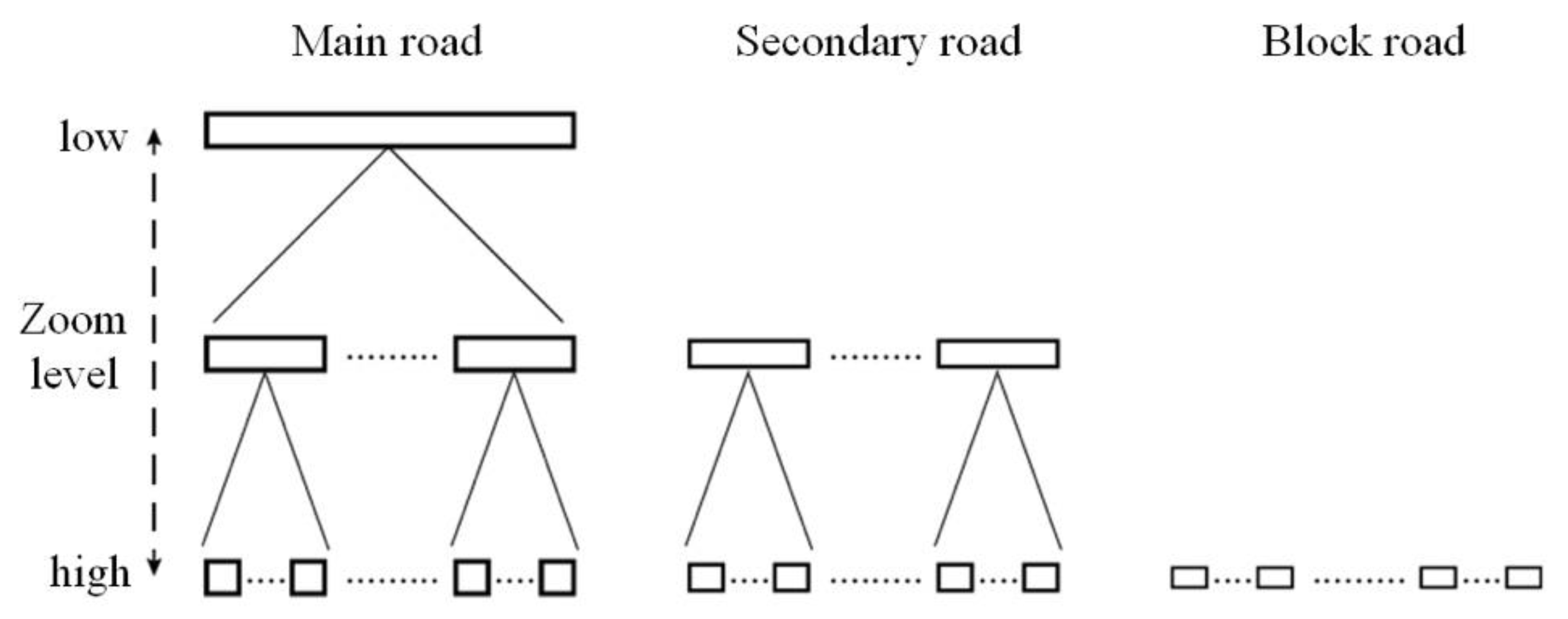
The visual representation of the road network is shown in Figure 7, where it has two significant changes in space; as the zoom level changes, the number of roads and the size of the section will change. For the study area, the appropriate scaling level is 12–15. For these two reasons, the system classifieds the level of the road network in the study area as presented in

Table 4. Road visualization hierarchy.

LOD	Grade	OSM Road Type (and It’s Level)	Minimum Visible Scale
1	Main road	‘trunk’: 1,’trunk_link’: 1	Zoom >= 12
		‘primary’: 2,
		‘primary_link’: 2
		‘secondary’: 3,
		‘secondary_link’: 3
2	Secondary road	‘tertiary’: 4,	Zoom >= 12.5
		‘tertiary_link’: 4
		‘residential’: 5
3	Block road	‘living_street’: 6	Zoom >= 14
		‘pedestrian’: 7

.

In the study area, the system provided five granularities for visualization: road section, 500 m, 200 m, 100 m, and 50 m. In addition to the road section, the maximum granularity size was 500 m, and the main constraints were the average length of the road section and the spatial distribution of waterlogging; the minimum granularity size was 50 m, and the main constraints were the map illustration limit. In Table 4, we can also see that there was an inclusion relationship between the particle sizes of the sub-section at different scales. Therefore, the waterlogging of the high-grade sub-section can be merged from multiple low-level sub-sections, which saves system computing power more than repeated segmentation of different granularity. A reasonable sub-section coding structure helps to sort out the inclusion relationships seen at all levels, which is convenient for the implementation of the above algorithm.

(2) Temporal granularity

Dynamic visualization involves the following parameters: (1) Data time range; (2) Data timestamp interval per frame; and (3) Switching time per frame. For this system, the time granularity mainly refers to the data timestamp interval of each frame. There is a brief introduction to the settings of the above three parameters. The time range is usually a complete rainstorm waterlogging process, which can also be adjusted to the period of interest according to the user’s needs; and the data timestamp interval of each frame depends on the highest data update frequency available. The urban waterlogging simulation module of this system can provide the waterlogging forecast every 10 min, therefore, the minimum time granularity is 10 min; the switching time of each frame depends on the user’s cognitive efficiency. The default is one second, but this can be adjusted by the user.

4.2. Prototype System of Road Waterlogging Visualization

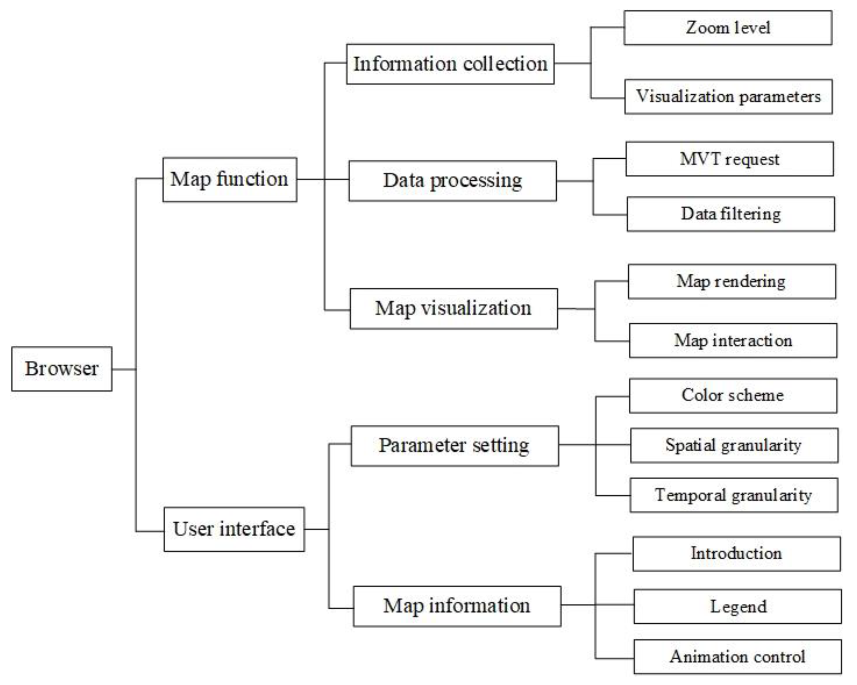
Based on the requirements of the system for cross-platform, publishing the information as a WebGIS page is a good choice. We selected MapBox GL JS as the visualization framework based on the following three considerations: (1) In combination with MVT (Mapbox Vector Tile) technology, it can reduce the burden of data loading in visualization and realize the rapid loading of spatio-temporal data; (2) By combining with MapBox Studio, map design can be carried out through an interactive platform, ensuring the beauty of map rendering and improving map usability; and (3) By using WebGL, cross-platform access is realized, and the possibility is reserved for subsequent 3D visualization. The core architecture of the visualization module is shown in Figure 8.

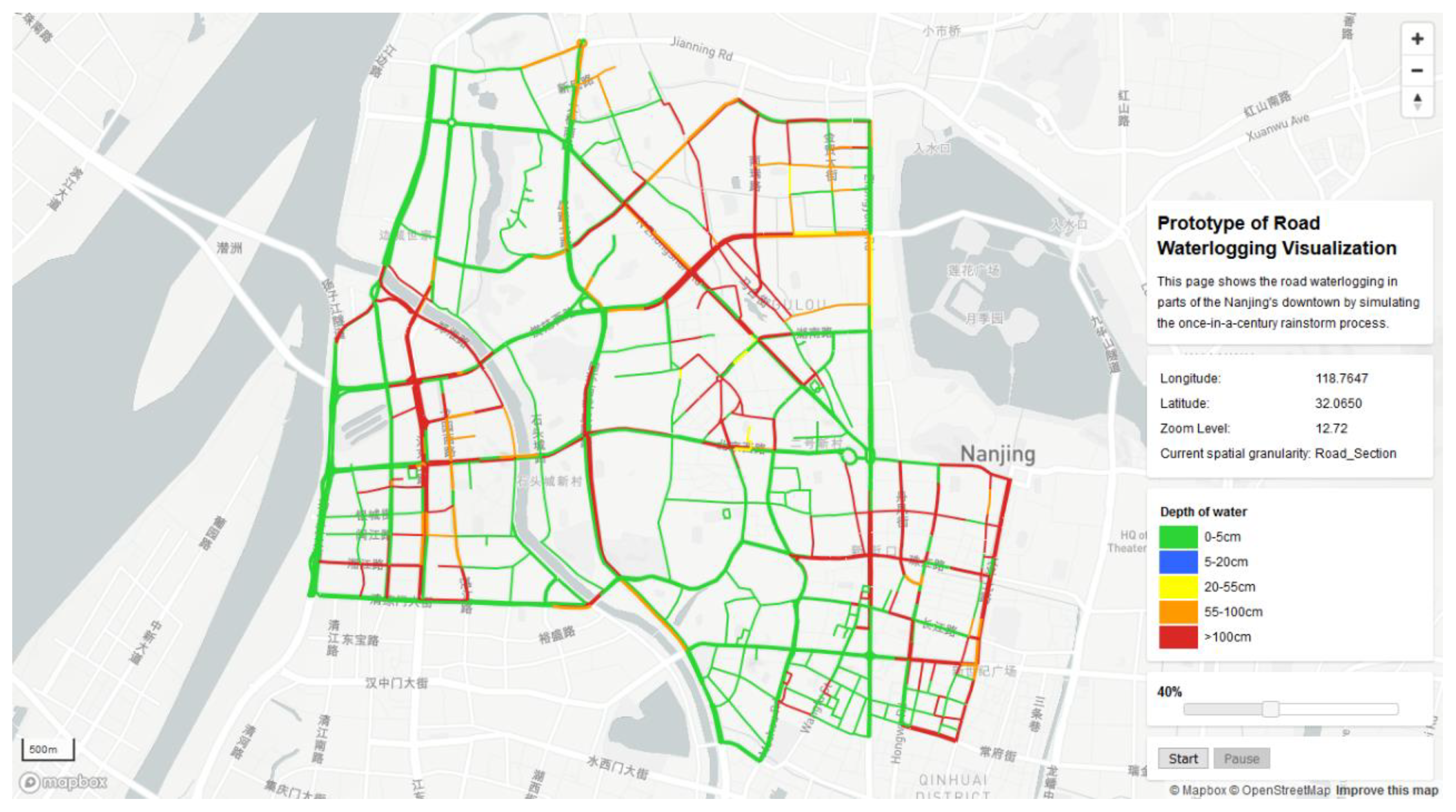
The visualization interface through the user’s web browser, as shown in Figure 9, mainly includes two parts.

(1) Map information

Map rendering in the Canvas container of the web page via Mapbox GL. Use “light-style” as the base map, and superimpose the road water layer on this basis. In addition to the main body of the screen, it also includes (1) a navigation control bar, located at the upper right of the interface, providing the function of zooming and rotating the base image; (2) scale bar, located at the lower left of the interface; and (3) map copyright information, located at the bottom right of the screen.

(2) Auxiliary information

Based on the basics of cartography, supplementary map essentials and control buttons necessary for dynamic visualization include (1) Title; (2) Information under current view such as latitude and longitude, zoom level, spatial granularity; (3) Legend; (4) Time progress bar; and (5) Animation playback switch.

4.2.1. Practical Effect of Granularity Segmentation

(1) Spatial granularity

The performance effect of spatial granularity is based on the spatial granularity calculation model proposed in Section 3.4.1. In this system, the following effects are more significant:

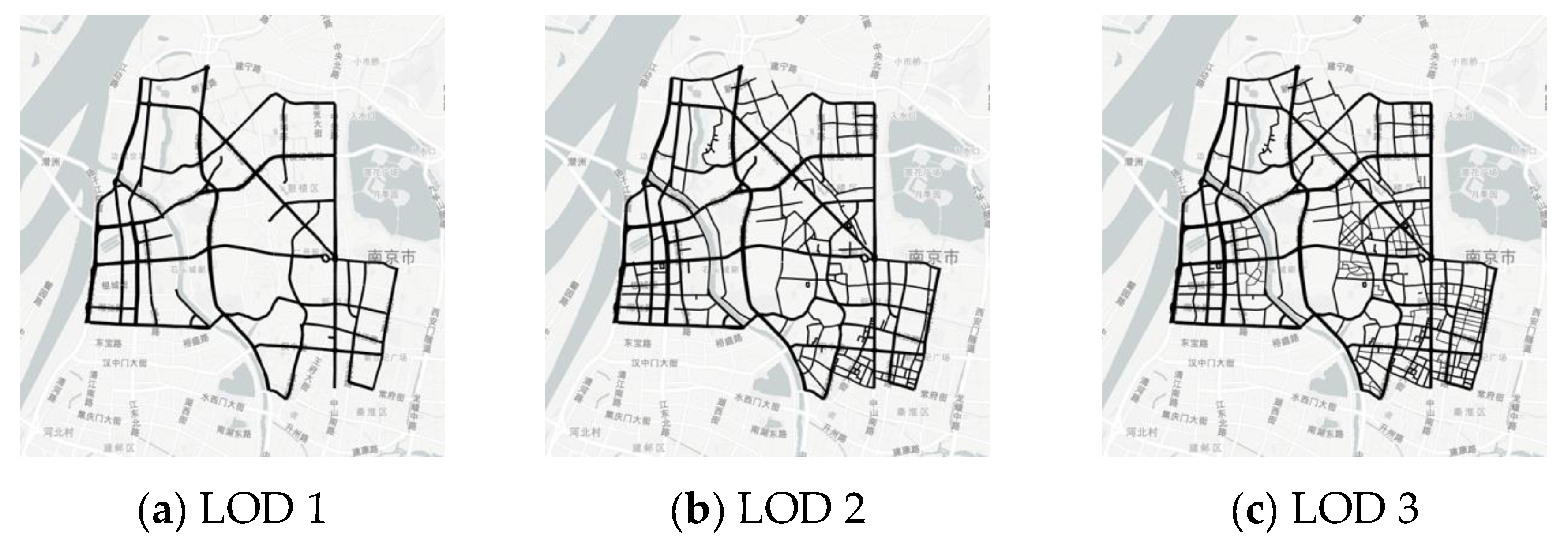
① Road network hierarchy

Based on Table 4, the road network has different display contents under different zoom ratios. In this study area, its display effect is as shown in Figure 10:

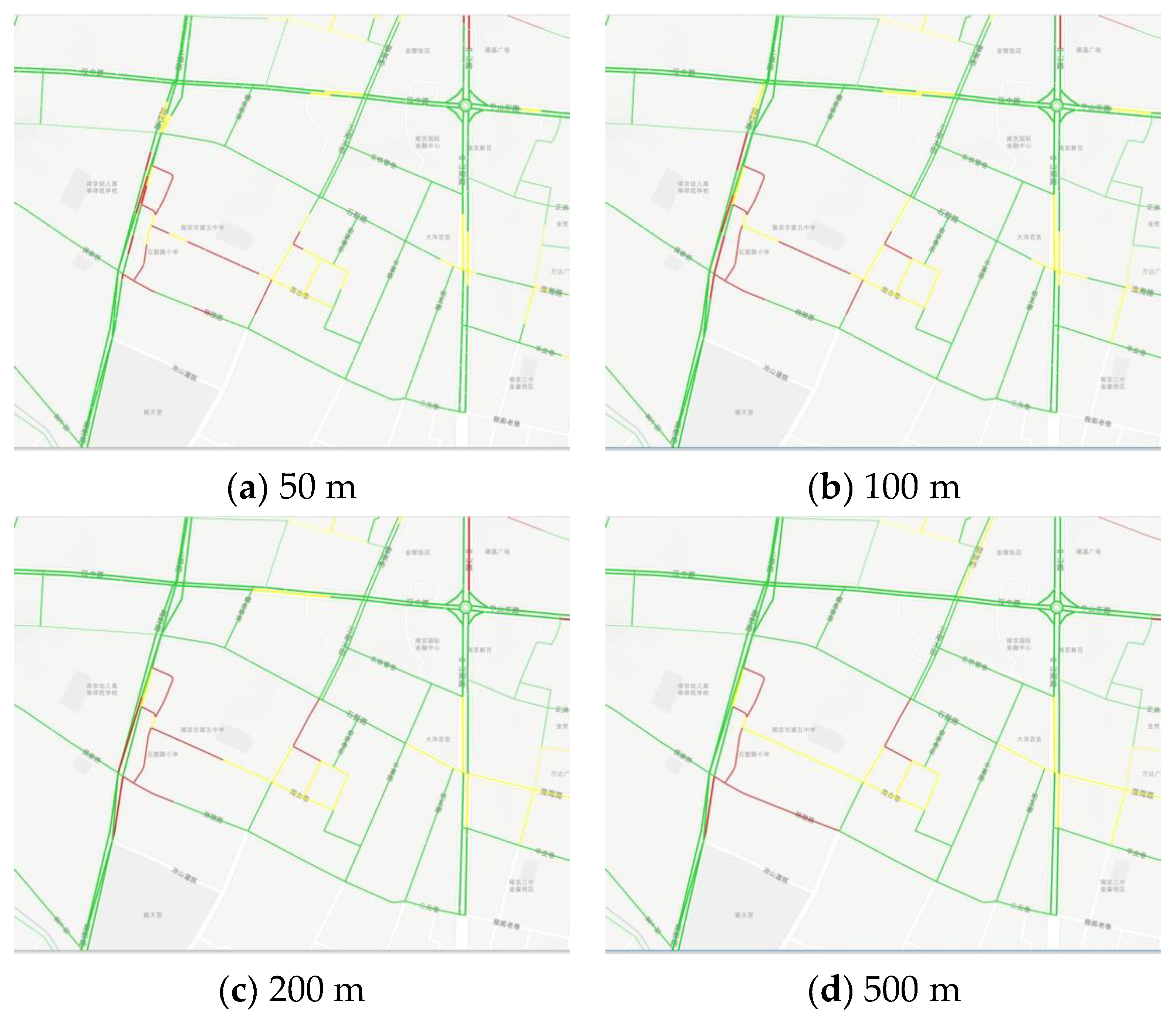
② Sub-section length change

The sub-segment lengths are different under different scaling ratios. In this study area, the effect is as shown in Figure 11.

(2) Temporal granularity

The performance of temporal granularity is based on the temporal granularity calculation model proposed in Section 3.4.2. In this system, the following aspects are more significant:

① Data timestamp interval per frame. To ensure the smoothness of the animation, the data timestamp interval of each frame should be as low as possible, and the data update frequency is limited to 10 min.

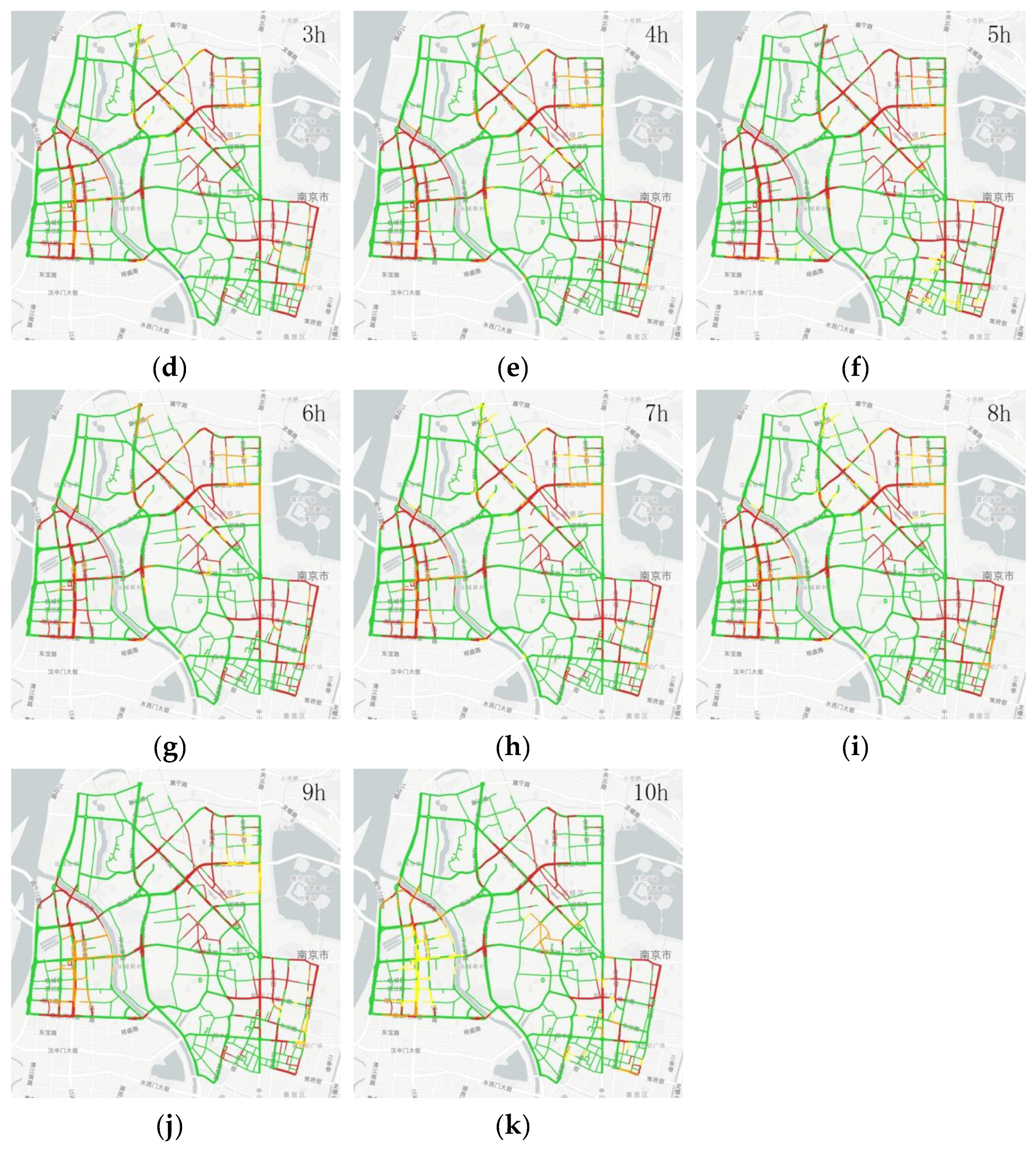
② Switching time per frame. The switching speed of the animation is greatly constrained by the user’s cognitive efficiency. After analysis, the range of values can be more appropriate from 500 milliseconds to 2000 milliseconds, with the default of 1000 milliseconds. Figure 12 shows the complete process of a rainstorm waterlogging lasting 10 h in the study area, expressed in 0 h–10 h, and dynamic visualization in hours (Scheme 1 in color scheme selection Table 2):

4.2.2. User Survey

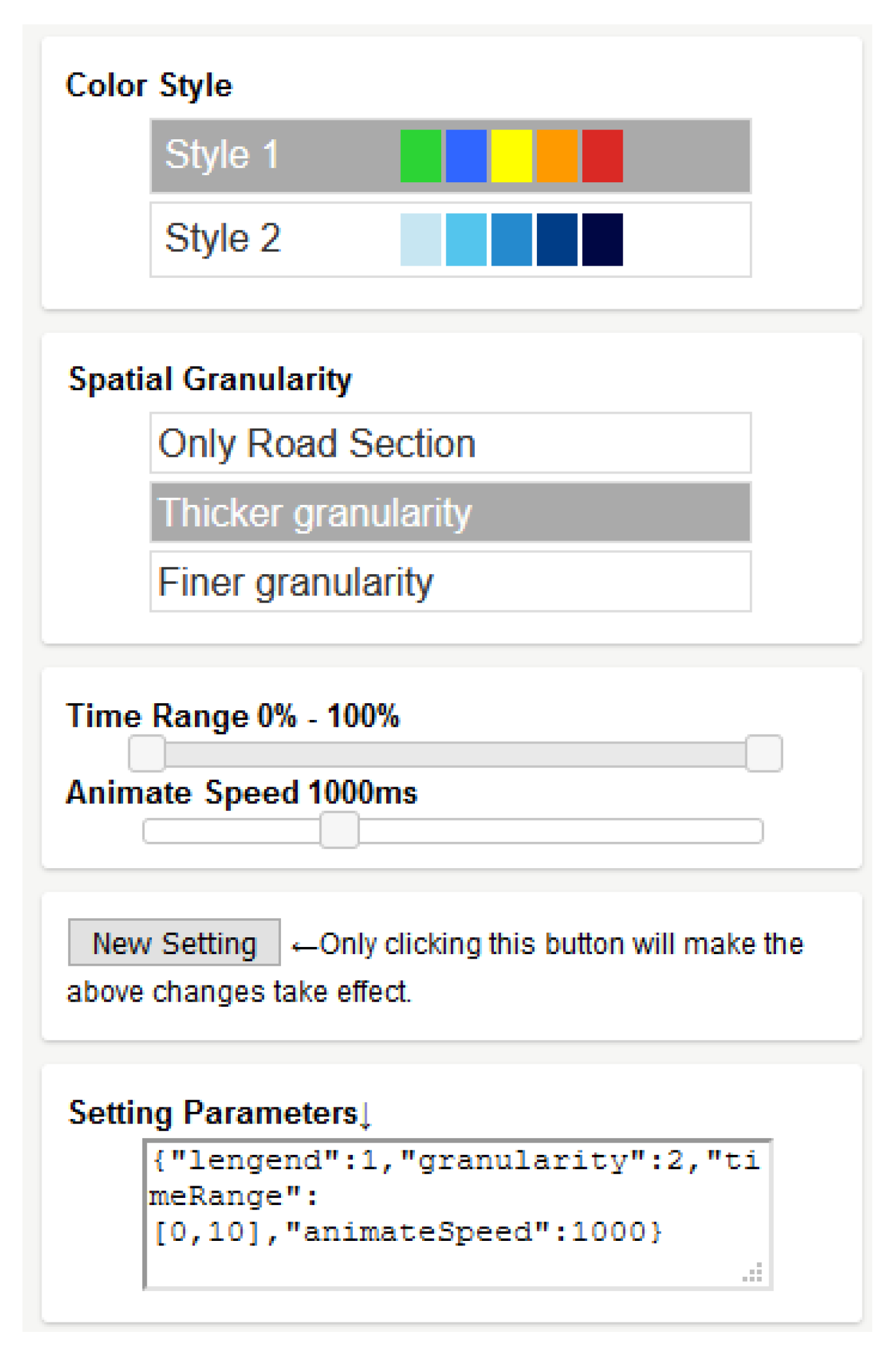
(1) Experimental purpose

In Section 4.2.1, the actual effect of the prototype system is shown from the two aspects of spatial granularity and time granularity. To verify the satisfaction of map users with the spatio-temporal visualization method proposed in this paper, a user test experiment was designed. First, we designed the user interaction function area, as shown in Figure 13. The user can freely select various parameters related to the visualization effect including: (1) Color style: allowing the user to freely select two color schemes of road waterlogging provided by the system; (2) Spatial granularity: the user can select three schemes of the original road section, coarse-grained road network, and fine-grained road network; and (3) Time granularity: the user can select the time range and playback speed of road waterlogging.

(2) Experimental process

A total of 32 participants were invited to participate in the experiment, all with an educational background in cartography and visualization. Before the experiment, we explained the possible influence of each parameter on the visualization effect through face-to-face or remote voice and text to participants, and then we let the participants try to adjust each parameter for about 5–10 min to feel the visualization effect of road waterlogging under different parameters until the user did not adjust the parameters and thought that the visualization effect of road waterlogging at this time was the best setting in the users’ mind, then the parameter settings were saved in the JSON (JavaScript Object Notation) string to collect the final parameter setting information of each participant.

(3) Experimental results and analysis

Results are as shown in

Table 5. Results of the user survey.

No.	Parameter	Optional	Number of Users Selected	Ratio
1	Color	Scheme 1	23	72%
		Scheme 2	9	28%
2	Road sub-section	1. Segment only	5	15.6%
		2. Thicker granularity	14	43.8%
		3. Finer granularity	13	40.6%
3	Time range	0–10 h	69% chose 10 h
4	Frame interval	100–3000 ms	75% in 640–1295 ms

, where the experimental results showed that 72% of the users preferred color scheme 1, where different color systems with distinct differences were used to visualize the depth of road waterlogging. A total of 15.6% of the people thought that for the visualization of road waterlogging, there was no need to divide the road sections using the original road network data, but 84.4% of people still set the parameters of spatial granularity, and thought that the segmentation of sub road sections was conducive to the visualization of road waterlogging, but for the selection of coarse-grained and fine-grained, there was no significant tendency. A total of 69% of people chose the playback range of 10 h, which means that most people were willing to observe a complete waterlogging process, and 75% of the people chose the playback speed of 640–1295 ms, which is close to the default 1000 ms setting of the system. In conclusion, participants generally gave a positive evaluation of the usability of the prototype system.

5. Discussion

The subject of this study was a spatio-temporal visualization method of urban waterlogging early warning based on dynamic grading. To focus on this research goal, first, we extracted the road waterlogging depth, which was provided by the Jiangsu Meteorological Service Center, but because the data provided were in raster format, it needed to match with the vector road network. The depth of road waterlogging provided by them was based on the spatial average elevation. However, we got the high-precision DEM data in the study area and we proposed a method to segment the road to correct the original road waterlogging data. First, we extracted the center point of a small road section as the sampling point and calculated the deviation value between the real elevation and the average elevation of the sampling point to correct the original road waterlogging data and obtain the revised road waterlogging depth information.

Second, we scientifically divided the depth of road waterlogging into five levels and set up two color schemes according to the cognitive habits of users. The first scheme was color matching of different color systems, where the color was from cold to warm, so the waterlogging depth started as less green, and gradually changed to red with the increase of depth, which gives people a relatively tense visual feeling, representing the level of road waterlogging to attract the users’ attention at this time. Scheme 2 was color matching of the same color system. In users’ cognitive habits, blue is an easy color to associate with water, and the darker the color, the deeper the waterlogging. In the user cognitive test experiment, 72% of people preferred Scheme 1 with the different color systems.

Third, the problem of granularity in the spatio-temporal visualization of road waterlogging is specifically about the length and time interval of spatio-temporal segmentation.

(1) Spatial granularity: there are two significant spatial changes in the multi-scale and multi-level road network structure, and with the change in scale level, the number of roads and the size of road sections will change. However, the division distance of sub sections cannot be infinitely reduced, which will lead to an increase in data volume. In this experimental area, five kinds of division granularity are provided: road section, 500m, 200m, 100m and 50m.

(2) Temporal granularity: the time range is usually a complete process of the rainstorm and waterlogging. The timestamp interval of each frame depends on the highest data update frequency available. As the Jiangsu Meteorological Service Center can provide a waterlogging forecast every 10 min, the minimum time granularity as set to 10 min, and the switching time of each frame is dependent on the user’s cognitive efficiency. The default value is one second, but the user can adjust it accordingly.

Finally, we constructed a prototype system of spatio-temporal visualization for waterlogging warning. To verify the satisfaction of map users with the spatio-temporal visualization method proposed in this paper, we designed a user test experiment. For about 5–10 min, users tried to adjust various parameters (color style, spatial granularity, temporal granularity) to feel the visual effect of road waterlogging under different parameters and the results finally showed that most users were willing to observe a complete process of waterlogging and 75% of the users chose the playback speed of 640–1295 ms, which was close to the default 1000 ms setting of the system. A total of 84.4% of the users set the parameters of spatial granularity, and thought that sub section segmentation was helpful to the visual expression of the road waterlogging, but for the selection of coarse-grained and fine-grained, there was little difference and no significant tendency.

6. Conclusions

This paper implements an approach to visualize the waterlogging of roads in spatio-temporal dimension, especially the research on the spatio-temporal granularity of road waterlogging visualization. To address the lack of thematic maps that show the impact of the urban waterlogging on road traffic in the vector format, we proposed the spatio-temporal dynamic grading and visualization method for road waterlogging warning, and a prototype system was designed to evaluate the proposed method. Results of the implementation and the experiment showed that the spatio-temporal visualization method of road waterlogging was positively correlated with the usability of urban waterlogging thematic maps. Spatio-temporal visualization of road waterlogging helps to provide scientific support for the disaster prevention and mitigation department and the traffic management department to specify emergency strategies, helps the public understand the road status and accumulated water information as well as adjust their travel plans.

In the future, we will consider the combination of the early warning of road waterlogging and traffic flow. The main function of road waterlogging warning is to provide auxiliary information for urban citizens’ in their travel decision-making. Therefore, one consideration can be to switch multiple visual variables to express the road condition and waterlogging comprehensively, which will greatly improve the usability of the system. Furthermore, the data model sensitivity study should be approached and improve the adaptivity of the model to different resolutions of DEM and frequent weather data.