A Framework Uniting Ontology-Based Geodata Integration and Geovisual Analytics


1
KRDB Research Centre, Faculty of Computer Science, Free University of Bozen-Bolzano, 39100 Bolzano, Italy
2
Chair of Cartography, Department of Aerospace and Geodesy, Technical University of Munich, 80333 Munich, Germany
3
Ontopic S.r.L, 39100 Bolzano, Italy
4
Department of Computing Science, Umeå University, 901 87 Umeå, Sweden
*
Author to whom correspondence should be addressed.
ISPRS Int. J. Geo-Inf. 2020, 9(8), 474; https://0-doi-org.brum.beds.ac.uk/10.3390/ijgi9080474
Submission received: 10 May 2020
/
Revised: 6 July 2020
/
Accepted: 27 July 2020
/
Published: 28 July 2020
(This article belongs to the Special Issue On Denotation and Connotation in Web Semantics, Collaboration and Metadata)
Abstract
:In a variety of applications relying on geospatial data, getting insights into heterogeneous geodata sources is crucial for decision making, but often challenging. The reason is that it typically requires combining information coming from different sources via data integration techniques, and then making sense out of the combined data via sophisticated analysis methods. To address this challenge we rely on two well-established research areas: data integration and geovisual analytics, and propose to adopt an ontology-based approach to decouple the challenges of data access and analytics. Our framework consists of two modules centered around an ontology: (1) an ontology-based data integration (OBDI) module, in which mappings specify the relationship between the underlying data and a domain ontology; (2) a geovisual analytics (GeoVA) module, designed for the exploration of the integrated data, by explicitly making use of standard ontologies. In this framework, ontologies play a central role by providing a coherent view over the heterogeneous data, and by acting as a mediator for visual analysis tasks. We test our framework in a scenario for the investigation of the spatiotemporal patterns of meteorological and traffic data from several open data sources. Initial studies show that our approach is feasible for the exploration and understanding of heterogeneous geospatial data.
1. Introduction
In a variety of applications relying on geospatial data, getting insights into heterogeneous geodata sources for decision making is crucial and has attracted a lot of attention. Visual analytics is a booming and promising research field dedicated to interactive graphic exploration of large and complex data facilitated by automated computational methods [1,2]. It has been noticed that effective visual analysis requires large and complex data organized in a coherent way and with clear semantics. In particular, the visual analytics research community has identified two major challenges in data management for visual analytics, namely data integration and semantics management [2]. More specifically, they argued that “logic based systems, balancing expressive systems power and computational cost represent state of the art solutions. Visual analytics can greatly benefit from such an approach [...]” and “associated with data integration activities, is the need for managing all the data semantics in a centralised way, for example, by adding a virtual logic layer on top of the data itself”.
The problem becomes more prominent in the big data era. With the pervasive usage of location positioning and communication technologies, huge amounts of geospatial data are collected on a daily basis, for instance, movement trajectories, geo-tagged social media texts, and images. Those data are in a variety of formats, ranging from structured, over semi-structured, to unstructured, and they represent a variety of geospatial phenomena. While most existing visual analytical systems are only able to deal with geospatial big data of particular types, developing visual analytical approaches that can directly apply visualization methods to data of different formats, representing different kinds of phenomena, is still challenging. This problem is acknowledged in the geovisual analytics community [3], where it is stressed that variety is one of the key issues in the research agenda related to visual analytics in the context of geospatial big data. They recognized “the significant analytical potential that can come from diverse data representing different perspectives on a problem” and suggested that “while the integration of geospatial big data is a problem, location can be used as a common denominator, and the linked data concept is also promising”.
The main research challenge that we address in this paper stems from the fact that it is getting increasingly difficult for geoscientists to express their analysis tasks. When working with geospatial phenomena, geoscientists are used to think in terms of the core concepts from the GIS domain, e.g., position, time, observation, and event [4]. The goal of (visual) analytics is essentially to understand the relations existing among these concepts. However, in reality, geoscientists have to deal with data structured and organized in possibly many different ways, so that the correspondence between these data and the core concepts of interest to the scientists is often unclear. Making this correspondence explicit requires a huge effort in finding the appropriate data, and in cleaning and preparing it for analysis. However, these should not be the core tasks of geoscientists. For instance, Equinor (previously Statoil), the Norwegian oil company, reported that the geologists in the exploration department have to spend up to 70% of their time in finding and preparing data, instead of carrying out their analysis itself [5]. The problem above is due to the fact that geoscientists are usually forced to work at a too low level of abstraction and there is a big semantic gap between the raw data and the terms that are commonly adopted in their professional domain. For example, in order to aid in the exploration of oil, oil companies drill wellbores, which are the holes that form the well, and during the drilling they collect a huge amount of data, which will be managed by the IT department. When the geologists analyze such data, they have to know that in order to get all the meaningful wellbores, they need to look into the table WELLBORE and, more importantly, the value of a specific column, namely REF_EXISTENCE_KIND, has to be ‘actual’, but not any other value [6]. Such knowledge is normally only known to the IT management team but not to the geologists. We argue that this challenge of the semantic gap is not merely an engineering problem, it has to do with how geo-concepts and raw data sets are related, and addressing it in an adequate and general way requires both new methodologies and techniques.
In this work, we attempt to fill the above mentioned research gap by resorting to ontology-based data integration (OBDI) and applying it to visual analytics. OBDI aims at providing a (virtual) coherent ontological view of the underlying heterogeneous data, and hence is well suited to be combined with visual analytics in order to facilitate analysis and decision making. Specifically, we propose an ontology-based framework (called Ontology-based Geodata Integration for Geovisual Analytics (GOdIVA)) for data integration and analysis, which consists of two modules centered around an ontology: (1) an OBDI module, in which mappings specify the relationship between the underlying data and a domain ontology; (2) a geovisual analytics (GeoVA) module, designed for the exploration of the integrated data, by explicitly making use of standard ontologies that are defined by standard organizations, or are de-facto standards used in certain domains.
Compared with classical analytics frameworks, ontologies play a central role in the GOdIVA framework by decoupling the challenges of data access and analytics: on the one hand, the ontology layer provides a coherent view over the data in the sources, abstracting away the details of how such data are structured; on the other hand, it acts as a mediator for analysis tasks and visual exploration of spatiotemporal patterns. In this paper, we rely for the OBDI module on the common practice of building the ontology by reusing and extending standard ontologies, e.g., the GeoSPARQL ontology [7] for spatial features and relations, the Time ontology [8] for temporal entities and relations, and the Semantic Sensor Network (SSN) ontology [9] for sensors and observations. The adoption of such standard ontologies also facilitates the reuse of the tools developed for the GeoVA module.
With the GOdIVA framework we attempt to manifest a double value-adding process required in the era of big data. Ontology-based integration of heterogeneous data sources is internalized as a fundamental effort towards a universally interoperable and manageable geodata infrastructure, whereas geovisual analytics supports the externalization of the integrated data back to diverse but easily comprehensible visual expressions. What is new is neither the approach of ontology-based integration nor the geovisual analytics, rather a united form of the two.
We developed a prototype of the framework in a web-based visual analytical system relying on the OBDI system Ontop [10] and carried out an experimentation in a scenario investigating the spatiotemporal patterns of and the correlation between meteorological data and traffic data in the area of South Tyrol, Italy. To do so, we used the GeoSPARQL and SSN ontologies to integrate the time-series and observation data from several open data sets provided by the Open Data Portal of South Tyrol (http://daten.buergernetz.bz.it/de/) and by the State Institute for Statistics of the Autonomous Province of Bozen-Bolzano (ASTAT) (http://astat.provinz.bz.it/de/default.asp). Our studies show that the GOdIVA approach can indeed be adopted for exploring and understanding heterogeneous geospatial data.
The rest of the paper is structured as follows: In Section 2, we provide background knowledge and survey related work. In Section 3, we present our framework in detail. In Section 4, we describe a case study integrating and analyzing data from several open data sources. In Section 5 we conclude the paper and discuss further research challenges and opportunities.
2. Background and Related Work
In this section, we provide background knowledge and discuss several research directions relevant to this work.
2.1. Ontology-Based Geospatial Data Integration
Geospatial data integration is the key technology to achieve the added value from heterogeneous data sources to the geovisual services [11,12]. Semantic integration has gained considerable attention in geographic information system (GIS) interoperability with the goal of conquering semantic heterogeneity [13,14].
At the core of solutions based on Semantic Technologies we typically have an ontology. In computer science, the term “ontology” denotes a concrete artifact that conceptualizes a domain of interest and allows one to view the information and data relevant for that domain in a coherent way shared among all actors interested in that domain. Such ontologies (which we call domain ontologies) are typically designed and used with a specific purpose in mind, as opposed to having the objective of capturing general notions about the world. To simplify the sharing and reuse of ontologies, the World Wide Web Consortium (W3C) (http://www.w3c.org/) has defined standard languages in which to express them. We refer here to Resource Description Framework (RDF) [15], providing a simple mechanism to define the vocabulary used in a specific domain, and Web Ontology Language (OWL) [16], providing a very rich language in which to encode complex conditions that hold in the domain of interest. These two standards are important, on the one hand because Open Data becomes increasingly available as knowledge graphs in RDF [17], and on the other hand because many domain ontologies expressed in OWL have been standardized. For instance, the Spatial Data on the Web Interest Group (https://www.w3.org/2017/sdwig/), a joint effort of both W3C and Open Geospatial Consortium (OGC), is working specifically on sharing spatial data on the Web using Semantic Web technologies. Their activities include standardizing the Time ontology [8] and the Semantic Sensor Network (SSN) Ontology [9], and maintaining the GeoSPARQL ontology [7].
In the past two decades, the ontology-based approach has been widely used in the GIScience domain to overcome semantic integration obstacles by an explicit and formalized representation of semantics [18,19,20]. Many researches proposed geo-ontologies to represent domain knowledge and support geospatial data integration in applications like trajectory mining [21], earthquake emergency response [22], and oceanographic data discovery [23]. Other examples of such ontologies are developed to support the tasks of geographic information discovery [24], retrieval [25], and integration [26]. Most of these works integrate the geodata sources by converting original data and materializing them as RDF, and then storing them in a triple store. This way of proceeding is expensive when datasets are large or when the data change frequently.
Ontology-based data access (OBDA), also known as Virtual Knowledge Graph in the literature, is a popular paradigm that enables end users to access data sources through an ontology. The ontology is semantically linked to the data source by means of a mapping consisting of a set of mapping assertions [27]. The standard mapping language is R2RML [28]. Thus, the ontology and mapping together, called an OBDA specification, expose the underlying data source as a virtual RDF graph, and makes it accessible at query time using SPARQL. The virtual approach avoids the high cost of materialization.
Ontology-based data integration (OBDI) is an extension of OBDA in which data are not originally in a single data source, but come from multiple data sources that need to be queried in an integrated way. OBDI typically requires an additional step of setting up an (integrated) database so that one can issue SQL queries to multiple data sources at the same time. This can be done by either using a SQL federation engine, e.g., Denodo (https://www.denodo.com/) or Dremio (https://www.dremio.com/), to connect to the existing databases, or using a more straightforward “physical integration” approach to import all the datasources into one database system. After this step, OBDI maintains the same conceptual architecture as OBDA [29]. OBDI systems implementing this paradigm include Mastro (http://www.obdasystems.com/it/mastro/) [30], Morph (https://github.com/oeg-upm/morph-rdb/) [31], Ontop [10], Stardog (https://www.stardog.com/), and Ultrawrap (https://capsenta.com/ultrawrap/) [32]. Recently, Ontop has been extended to support GeoSPARQL [33]. Although not using the R2RML and OWL standards, the LinkedGeoData project [34] is a pioneer work which follows the principle of OBDI and converts the OpenStreetMap (OSM) data to an RDF graph and interlinks these data with other open RDF knowledge bases. OBDI has been used in many use cases [35]. In particular, it has been used for consistency assessment of open geodata [36], and for maritime security [37]. In this work, we rely on OBDI for geodata integration.
2.2. Geovisual Analytics
Geovisual analytics (GeoVA), derived from visual analytics [1], refers to the science of analytical reasoning with spatial information as facilitated by interactive visual interfaces [38]. It deals with problems involving geographical space and various objects, events, phenomena, and processes populating it [39]. GeoVA approaches are widely applied for the efficient exploration of big geospatial data, including movement trajectories [40,41,42], geo-tagged social media data [43,44], and sensor data streams [45].
Meaningful visual analytics of geodata still faces semantic challenges of heterogeneous information [3,46,47]. Some efforts have been done towards integrating domain ontology models as a knowledge representation component to visual analytics systems, e.g., for the management of bridge safety and maintenance [48], and in the analysis of trajectories [49]. Compared with the approach proposed in our paper, these works focused on particular use cases and did not carry out systematical studies on the issue of combining ontologies and visual analytics.
Ontology-based geovisual analytics systems require an interactive graphical user interface to visualize geo-ontologies and spatial RDF data. Katifori et al. [50] surveyed comprehensive visualization techniques for representing ontologies. Lutz and Klien [51] presented an approach for ontology-based retrieval of geographic information, and discussed the interface design. Several systems have been developed for visualizing RDF and SPARQL queries and results over spatial data. OptiqueVQS [52] is a visual query system for building SPARQL queries. GeoYASGUI [53] is a front end Javascript library for visualizing the results of GeoSPARQL queries on the map. Sextant [54] is a web-based system for the visualization and exploration of time-evolving linked geospatial data. Spex is a tool for exploratory querying of SPARQL endpoints in space and time [55]. Brasoveanu et al. [56] studied visualizing statistical linked knowledge for decision support. Huang and Harrie [57] proposed a knowledge-based approach to formally represent geovisualisation knowledge regarding cartographic scale, data portrayal and geometry source. See also the work by Dadzie and Pietriga [58] for a summary of recent research on visualization of linked data. Most of these researches are assuming that the data sources to be analyzed are already integrated, but we argue that integration and analysis are closely related and should be handled together in one framework. Moreover, most of these visualization tools try to cope with arbitrary ontologies, while we focus on standard ontologies so that we can develop more dedicated and appropriate visualizations.
2.3. Sensor Data Analysis
With the advances in sensor technologies, sensor (or geosensor) data have been increasingly collected for monitoring the environment and urban dynamics. For instance, networks of meteorological sensors are essential to monitor atmospheric processes, and to assess both long-term climate change and short-term weather events. Vehicle sensing technologies are prevalent in measuring real-time traffic situations, which can support decision making in public traffic management and individual travel planning. The integration of vast amounts of heterogeneous sensor data is helpful to understand the behavior of complex environmental phenomena [59].
Statistical analysis methods are commonly applied to analyze sensor data. In the transportation domain, many works have investigated the relations between weather conditions and traffic flows, for instance, on the influence of rainfall on road accidents [60], road safety [61]), and the effect of weather condition on traffic performance and air pollution [62]. In most cases, relevant heterogeneous data have to be preprocessed and spatially joined in advance for specific analysis tasks. Then statistical analysis methods are applied to derive statistical values. However, this spatial join is an ad-hoc integration of geodata, while a systematic way of doing it is largely missing.
There have been several previous works e.g., [63,64], inspecting the ontology-based approach for sensor data analytics. In these works data are materialized for ontology and rule-based reasoning, and thus the approach is not well suited when data are very large or dynamically changing. In contrast, we employ the virtual integration approach and rely on on-the-fly query translation. Another key difference is the means for finding patterns from large geodata and inferring high-level knowledge (e.g., events, correlations, or causalities). Previous approaches rely on a fixed set of predefined rules, while in our framework the visual interface offers users the flexibility of discovering patterns with the support of high-level query answering and user interactions guided by intuitive visualizations.
When dealing with sensor data streams in real-time, the classical SPARQL querying is not suitable as it only works with static RDF graphs. Stream Reasoning [65] is an area studying reasoning in real-time over continuous data streams. In particular, RDF Stream Processing (RSP) adopts RDF streams as data model and can express patterns to detect in the streams. As for the query language, several extensions of SPARQL with a continuous semantics have been proposed [66,67]. The W3C RDF Stream Processing Community Group (https://www.w3.org/community/rsp) is trying to define a common language, and identifies RSP-QL [68] as a reference model that unifies the semantics of the existing RSP approaches. In addition, plain SPARQL is often not expressive enough to model complex temporal patterns. To overcome this limitation, [69] proposed an expressive rule language based on Metric Temporal Logic. The current paper focuses only on static data retrieved through classical SPARQL queries, while the real-time aspect and more expressive temporal queries are left for future work.
3. GOdIVA: A Framework Unifying Ontology-based Geodata Integration and Visual Analytics
In this section, we present a comprehensive framework, called Ontology-based Geodata Integration for Geovisual Analytics (GOdIVA), for integrating and analyzing geospatial data. The GOdIVA framework consists of two main modules: (1) ontology-based geodata integration (OBDI) and (2) geovisual analytics (GeoVA).
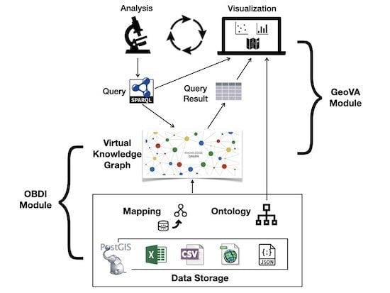
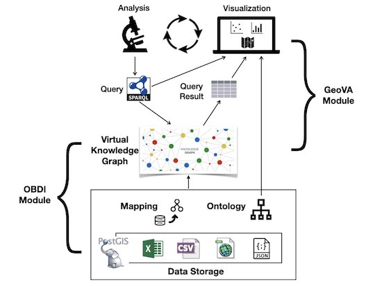
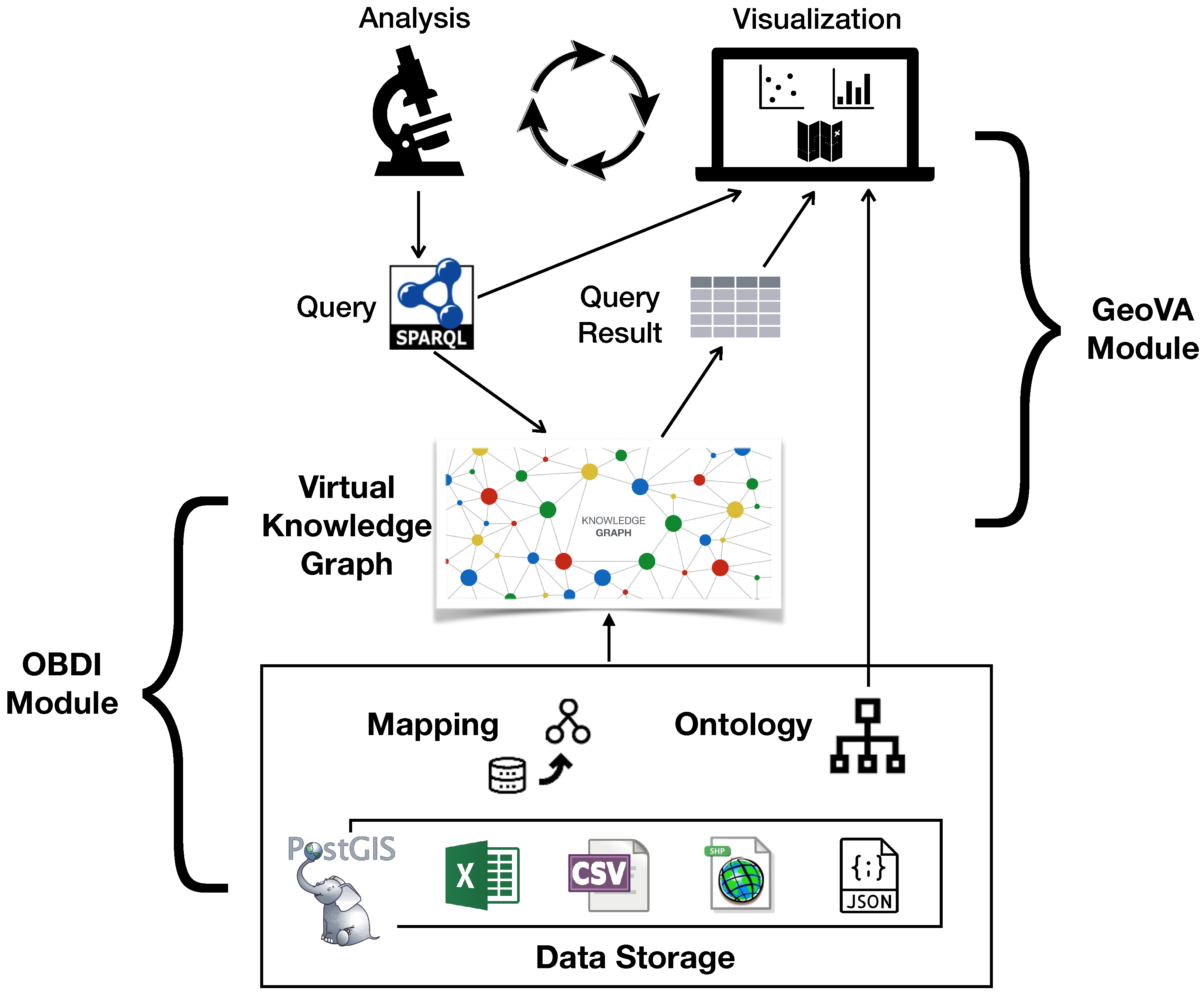
The framework provides the functionality to allow users to formulate their analysis tasks, in the GeoVA module, over the ontological representation of the underlying data exposed by the OBDI module. We depict in Figure 1 the structure of the two modules, where arrows indicate information flow. We now discuss briefly their main components. The OBDI module provides an ontological view over the datasets loaded in the data storage component. More concretely, a declarative mapping specifies how to populate the classes and properties defined in the ontology with the underlying data. The mapping and ontology together expose the underlying data sources as a unified virtual knowledge graph, which can be accessed via SPARQL queries. The GeoVA module allows users to visually interact with the virtual knowledge graph. The analysis tasks can be formulated as SPARQL queries using the vocabulary from the ontology. Then the query results, together with the ontology and queries, are presented to users using multiple visualization techniques. Following the iterative classical visual analysis pipeline [1], based on the visualization results, users can generate and perform new analysis and explore the data further. In the following subsections, we provide more details of these two modules.
3.1. Ontology-Based Geodata Integration Module
The OBDI module defines high-level concepts that model the domain of interest in terms of an OWL ontology [16]. The ontology models the underlying semantic concepts of the geospatial phenomena and can be used to guide the formulation of appropriate queries for the given purpose and data. The ontology hides the heterogeneity of the underlying data sources. The ontology-based data integration process is actually divided into two phases: (1) The physical integration phase is responsible for integrating raw data items into one geospatial database, and often requires data cleaning and format conversion. (2) The semantic integration phase provides an ontological view over the physically integrated geospatial data using the OBDI technology. The relationship between ontology and data sources is specified by declarative mappings. We pursue the virtual approach to OBDI, which avoids the materialization of the data in the ontology. Instead, queries formulated over the ontology vocabulary are answered by being translated on the fly into queries over the original sources, while performing also ontological reasoning.
The process of designing ontologies and mappings can be regarded as a documentation/annotation process over the data source. The construction of the ontology can be based on existing standard ontologies, e.g., GeoSPARQL [7] for features and geometries, and SSN [9] for sensors and observations. The ontology should reflect the nature of the studied spatial phenomenon. For instance, since the weather is a continuous spatial phenomenon (or field in the geosemantics community), we can add a property to associate the discrete observations to their stations, and also interpolate the observed values to a vector of grid data. This process of mapping and ontology construction is incremental and iterative: normally, we start with a small fragment of the data, and create an ontology and map data items into the ontological vocabulary. The initial fragment can be verified by observing query answers and visualization results. Then we deal with a larger fragment of the data. In this way, the construction combines both the inductive (bottom-up, data to ontology) and deductive (top-down, ontology to data) methodology. We remark that thanks to the virtual nature of our framework, we can avoid to explicitly materialize the data into the ontology, hence the (re)iteration of ontology/mapping construction step is much more lightweight than the materialization-based approach.
The OBDI module relies on standard formats in order to achieve interoperability, including R2RML [28] for mappings, OWL 2 QL [70] and RDFS [71] for ontologies, RDF [15] for the virtual graph, and SPARQL [72] and GeoSPARQL [7] for queries. Hence, any OBDI engine compatible with these standards can be used in this architecture. The OBDI setup is then exposed as a standard SPARQL endpoint, which implies that clients can communicate with the endpoint using the standard HTTP protocol [73].
3.2. Geovisual Analytics Module
The GeoVA module provides appropriate visual representations of the integrated ontological view of the underlying data sources, and guides the users to construct the analysis tasks to explore the data. In particular, the ontology can be used to select which visual analytics methods are suitable for the data sources [74]. The GeoVA module allows the analysts to concentrate on the relations between the ontological concepts. For instance, when the SSN ontology is employed, the users are ready to focus on the core concepts of “Platforms”, “Sensors”, and “Observations”, and a set of visualization methods relying on SPARQL queries can be developed dedicated for these concepts.
We also note that the decoupling of the OBDI module and the GeoVA module brings great reusability in designing visualization methods. Since the visualization methods only rely on the ontological representation, the GOdIVA framework is robust with respect to changes in the data source layer. Indeed when the ontology is stable, adding new data sources only requires adding more mappings from the new sources to the established concepts in the OBDI module, but the visualization methods in the GeoVA module can be reused.
The GeoVA module is designed to visually convey the following information: (1) the concepts in the ontology, and how they are related to each other, (2) the information needs in the form of SPARQL queries, and (3) the query results. The graphical interface should be designed to reflect the characteristics of these types of information [75]. Since an ontology normally contains a large number of concepts, which are often connected by complex relations, it is crucial to avoid overloading users with too much information about the ontology. Rather, the visualization should be designed centered around the key concepts and common patterns in the ontology [50]. The SPARQL language is based on graph pattern-matching, and basic graph patterns in SPARQL naturally have a graphical representation, which can be exploited. The query results normally contain rich information with spatiotemporal characteristics, which need to be revealed using visualization techniques focusing on different perspectives [45,74].
An effective geovisual analytics system requires a proper visual interface with a set of visualization and computation techniques that facilitate analytical reasoning. The visualization techniques are based on methods of cartographic visualization, information visualization, and other graphic representations [75]. For instance, heat maps are effective in conveying the spatial distribution of an ontological concept that captures a continuous phenomenon. These methods help to visualize the queried geodatasets in multiple ways and allow a synchronized visual exploration. The analytics functionalities support identifying patterns and deriving high-level knowledge (e.g., events and complex correlations). Statistical analysis methods can help abstract the queried results with statistical measures, like min, max values and correlation coefficients over ontological concepts, e.g., temperature and precipitation. These measures and their graphic representations provide users insights of the characteristics of the integrated geodata [38,76].
4. Case Study
We evaluate the GOdIVA framework on the use case of sensor data. More specifically, we integrate meteorological and traffic sensor data and visually analyze their spatiotemporal patterns and correlations. We store all the datasets in a PostGIS database. For OBDI, we build the ontology and the mapping using the Protégé ontology editor [77] with the Ontop plugin [10], and setup a SPARQL endpoint using Ontop. For GeoVA, we have implemented a web-based visualization system communicating with the SPARQL endpoint. The graphical interface is based on several popular Javascript libraries, including RDFLib.js (https://github.com/linkeddata/rdflib.js/), Openlayers (https://openlayers.org/), d3.js (https://d3js.org/), and vis.js (http://visjs.org/). The source code, including the documentation and data sets, is released on Github (https://github.com/dinglinfang/suedTirolOpenDataOBDA/).
4.1. Test Area and Data
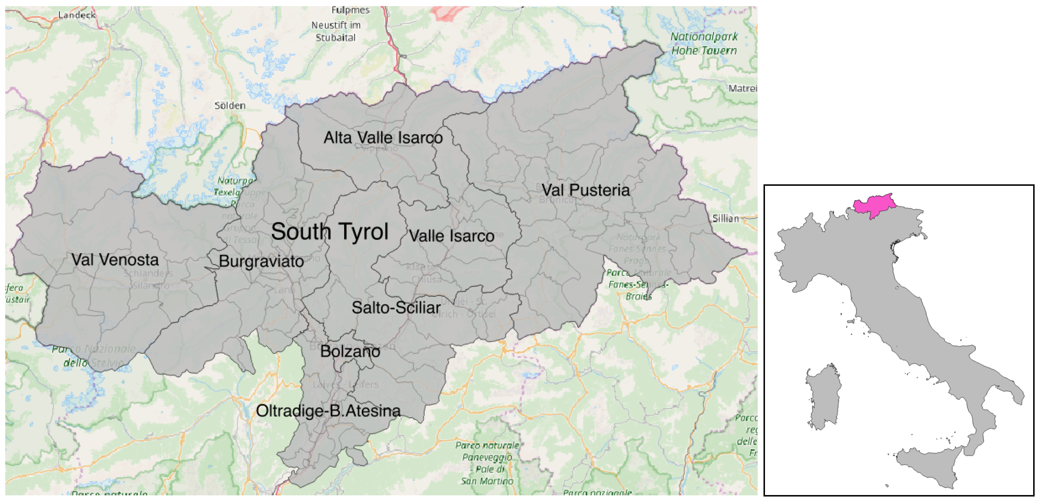
We use the province of South Tyrol (German: Südtirol; Italian: Alto Adige) in Italy as the test area. It is an autonomous province in northern Italy with two official languages, German and Italian. Figure 2 shows the geographic location of South Tyrol.
In this study, we use data from two data sources: (1) the Open Data Portal of South Tyrol (ODP) (http://daten.buergernetz.bz.it/), and (2) The State Institute for Statistics of the Autonomous Province of Bozen-Bolzano (ASTAT) (http://astat.provinz.bz.it/). The ODP collects data from local authorities, companies, and relevant stakeholders. As of 20 April 2018, it has published 458 datasets covering 17 categories on topics like meteorology, culture, health. These data and their metadata are provided in different formats, e.g., JSON, XML, CSV, and PDF. The portal also features a Geocatalog portal (http://geokatalog.buergernetz.bz.it/geokatalog/), providing massive geodata on administrative boundaries, satellite images, and transportation networks. These geodata are available in the formats of ESRI SHP, AutoCAD, Google KML, or GeoJSON. The ASTAT coordinates the official statistical activities in the province. It provides an interactive database on its website (http://astat.provinz.bz.it/de/datenbanken-gemeindedatenblatt.asp), where users can interactively view and download socioeconomic data. Most data are in XLS or PDF formats.
In this use case, we use meteorological and traffic data available from ODP and ASTAT. More specifically, from ODP we download data of municipality boundaries, meteo stations, sensors, and measurements in the last 30 years from 1980 to 2017. From ASTAT we download traffic statistical data on traffic volume and speed in 2017. These datasets are organized in different structures and provided in diverse formats. Table 1 shows the details of these datasets. We physically integrate these data by converting them into relational tables and storing them in PostGIS.
In addition, since meteorological measurements are representatives of a continuous geographic phenomenon existing through space, in this study we model this phenomenon as a surface with each location a unique phenomenon value. More specifically, we partition the study area into grid cells and interpolate the grid surface with the meteorological data. Considering the size of the study area, we set the grid cell size to 1 km by 1 km, resulting in total 7793 cells inside the study area. Figure 3a shows the grid partition. We then apply interpolation algorithms to the meteorological measurement data. The interpolation process can be regarded as an interpolator generating an observation for each cell. For generating precipitation and temperature surfaces, we apply the widely used Kriging interpolation method. Figure 3b depicts the interpolated precipitation surface on 4 January 2017.
4.2. Ontology-Based Data Integration
We show how to construct ontology and mapping so as to use the OBDI module for integrating the datasets.
4.2.1. Ontology
To model the knowledge of sensor data, we build our ontology on top of two standard ontologies, namely GeoSPARQL (with prefix geo:) and Semantic Sensor Network (SSN, with prefixes ssn: and sosa:). The complete list of prefixes used in our ontology is shown in Table 2. Figure 4 depicts parts of the ontology as shown in the Protégé editor. In this study, the core classes that we are relying on are geo:Feature, sosa:Platform, sosa:Sensor, sosa:ObservableProperty, and sosa:Observation. To represent domain-specific entities, we have enriched the ontology as follows:
- We have created two classes :WeatherStation and :TrafficStation as subclasses of both sosa:Platform and geo:Feature.
- We have created five subclasses of sosa:Sensor, e.g.,:MinTemperatureSensor and :TrafficSpeedSensor.
- We have created five instances of the sosa:ObservableProperty class, e.g., <minTemperature> and <trafficSpeed>.
- We have introduced a class :GridCell extending geo:Feature to represent a seamless partition of a geographic area. Then we create the :Interpolator class as a subclass of ssn:System, whose instance is hosted on a :GridCell platform and interpolates instances of :Observation.
4.2.2. Mapping
We construct the mapping from the database tables to the ontology vocabulary. A mapping assertion takes the form
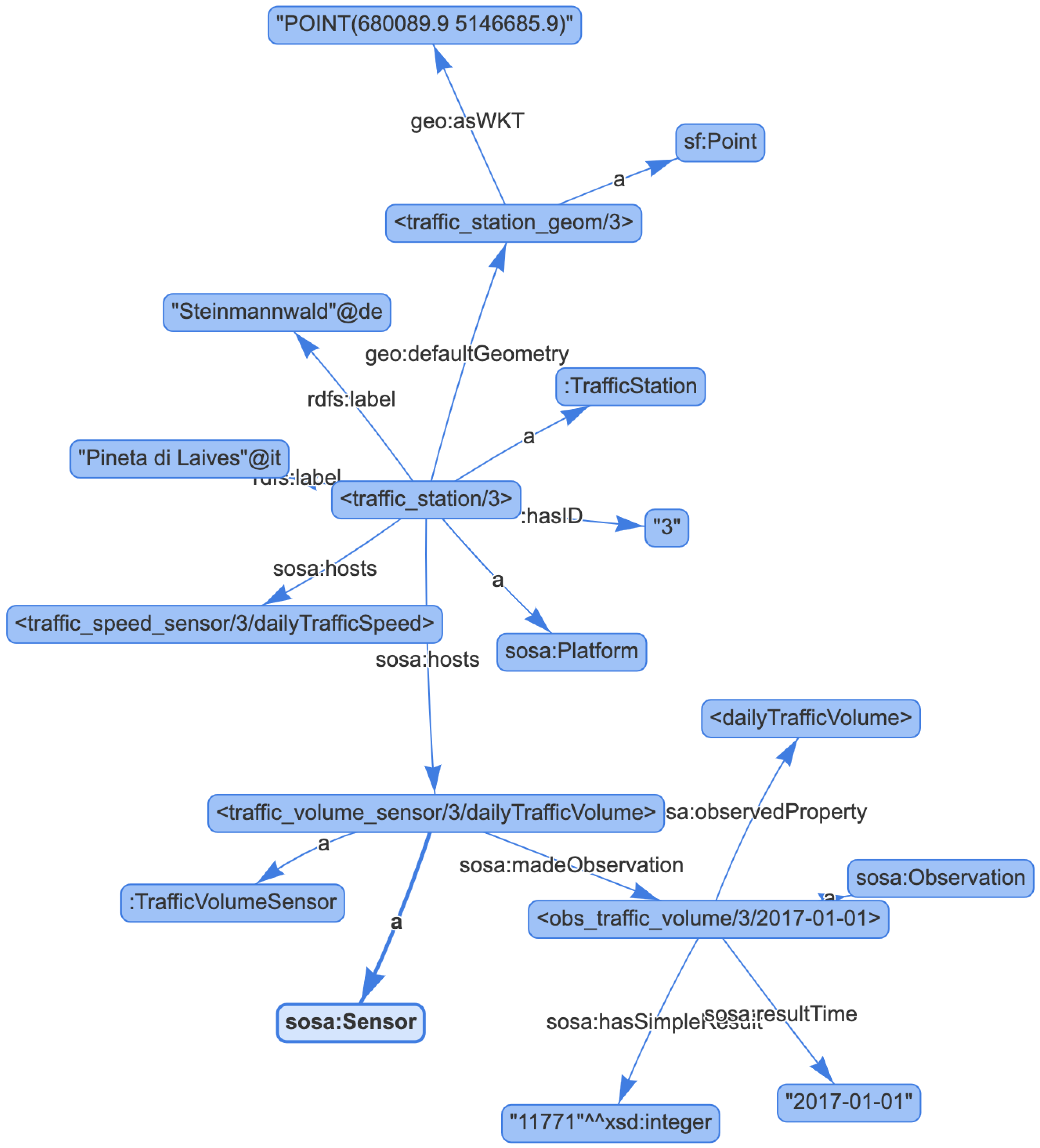
where id is an identifier, source is an SQL query, and target is a triple template. The target part contains placeholders like “{column}”, where column is an output column in source. In total we build 23 mapping assertions. In Table 3, the first column lists four example mapping assertions related to traffic stations, sensors, and observations, written in the Ontop mapping syntax [10], the second column shows sample data, and the last column shows triples generated by the mapping assertion over the sample data. For instance, consider the first mapping assertion M_traffic_station_info: since the answers to its SQL query over the database include (3, ‘Pineta di Laives’, ‘Steinmannwald’), it can generate the triples in the third column of the table. As the outcome of the integration, these four groups of triples, generated by the four mapping assertions over the sample data, form one connected RDF graph, as visualized in Figure 5. This clearly shows that these data sets have been integrated.
In addition to the triples generated explicitly by the mapping, the RDF graph is also enriched by the ontologial reasoning. For instance, Figure 5 includes the following two triples inferred by the ontology:
|
<traffic_station/3> a sosa:Platform . <traffic_volume_sensor/{station_code}/dailyTrafficVolume> a sosa:Sensor . |
Note that the triples generated by the mapping and ontology do not need to be materialized, but they are accessible via SPARQL queries using SPARQL-to-SQL rewriting techniques. By avoiding materializing the triples, adding new sources and modifying the OBDA specification becomes rather easy. In fact, the development of mapping and ontology is an iterative process: we adjust the mapping when we have a better understanding of the data. This shows that the virtual approach provides a large flexibility.
4.2.3. Query
The RDF graph, populated by the ontology and mapping over the database, can be queried with the SPARQL language using the vocabulary in the ontology. Query answering takes advantage of the ontological reasoning capabilities. For instance, when querying all the instances of sosa:Sensor, the system retrieves also all the instances of its subclasses in the ontology, e.g., :PrecipitationSensor and :TrafficSpeedSensor, using their SQL definitions in the mapping. In this way, the SPARQL queries are in general more understandable and more compact than their corresponding SQL versions. This aspect will be evaluated in Section 4.5, where also more example SPARQL queries are provided.
4.3. Geovisual Analytics
As a proof of concept, we have developed a web-based interactive system for the visual exploration of the observation data. The visualization is intended to show the following information: (a) the core concepts of the ontology, (b) the structure of SPARQL queries, (c) the spatial distribution of the stations, sensors, and meteorological observations, e.g., precipitation and temperature, (d) the temporal pattern of the observations in a defined time period, and (e) the potential spatiotemporal correlations among multiple observable properties. The designed visual interface and the set of visualization and statistical analysis methods are introduced below.
Visual interface. Corresponding to the tasks, we design the visual interface with four basic visual components, shown in Figure 6. It consists of four linked views:
- A data access and analysis view (upper left). This view lists the core concepts as information items, which connects the ontology model and SPARQL. Users can click/check the intended features to formulate a query to access data. The design of this view is basically according to the core vocabularies in the ontology, including stations, sensors, and observable properties. A time window is added to select data in a certain time slot. In addition, we add one functionality to allow the visual exploration of the correlations between weather and traffic data. At the moment, the view is hand-crafted, but we plan to automatically generate it in the future according to the ontology.
- A SPARQL query view (bottom left). This view is linked to the data access view. When the query is formulated and issued to the SPARQL endpoint, it draws a network graph of the SPARQL query, showing directly the basic graph patterns of the query. It allows an intuitive perception of the involved concepts and their complicated relations.
- A map view (upper right). The map view is linked with the data access view and the statistical view. It is designed to show the spatial distribution of queried objects, for instance, the locations of all the meteo-stations, and the precipitation distribution. In addition, users can interactively select a feature on the map to investigate its characteristics in the linked statistical view.
- A statistical result view (bottom right). It is linked to the data access view and the map view, and is designed to show relevant statistics of the selected feature on the map in the selected time period. We have designed three tabs, respectively showing the basic information of the selected feature (e.g., traffic station ID, and the min and max traffic volume at this station), the time series of the observations, and the correlation coefficients of the weather and traffic at this station.
In Figure 6, the query “traffic stations” on the data access view is executed to get all the traffic stations. Correspondingly, the formulated SPARQL query graph is visualized on the SPARQL query view, and the retrieved stations are shown on the map view. After selecting the station with the ID of 3, the statistics view shows its basic information and the min and max values of the traffic volume and traffic speed.
Visualization techniques. Multiple visualization techniques are employed in the system to show data in different perspectives, following cartographical principles [78]:
- Network visualization. The visualization consists of nodes and edges and is especially suitable to visualize the complicated objects and relations involved in SPARQL queries. Figure 6 shows the query graph after selecting the traffic station with the ID of 3 to retrieve all the relevant information of this station, in which blue-filled nodes are used to represent IRIs and literals, and unfilled ones are variables.
- Dot maps and Heat maps. Cartographic techniques are effective in conveying spatiotemporal patterns. We use dot maps to represent the distribution of the sensor and station locations, and heat maps to show the distribution surfaces of the continuous phenomena, e.g., precipitation and temperature.
- 2-D scatter and line plots. They are designed mainly to reveal the temporal patterns of the observations. The scatter plots can show the individual variable values of each day, while the line plots show the temporal trend over a time period.
- Interactive correlation coefficient matrix. The matrix view can show the overview of the calculated coefficient results among multiple variables. It helps the users to find significant correlations. A bipolar color scheme from blue to red is applied to represent the correlations from negative to positive values. Furthermore, users can click a cell in the matrix to investigate the scatter plot of the two selected variables.
Statistical analysis methods. We implemented several statistical computing operations to abstract the queried datasets with statistical measures including min values, max values, and correlation coefficients. Those values together with their graphical representations give users an intuitive view about the datasets [56].
- Aggregate functions. The aggregate functions mainly calculate the min, max, and average values of each variable. For example, at each traffic station, users can get a list of the basic statistical values. These values, like daily traffic volume values, give users an overview of the traffic flow at the station.
- Correlation coefficient analysis. Spatial and temporal correlations of multivariates from different sources are important for finding interesting patterns and inferring potential events. As a demonstration, we implemented the Pearson correlation coefficient (For two datasets and , the Pearson correlation coefficient is .) and visualize the coefficients as a matrix.
4.4. Analysis
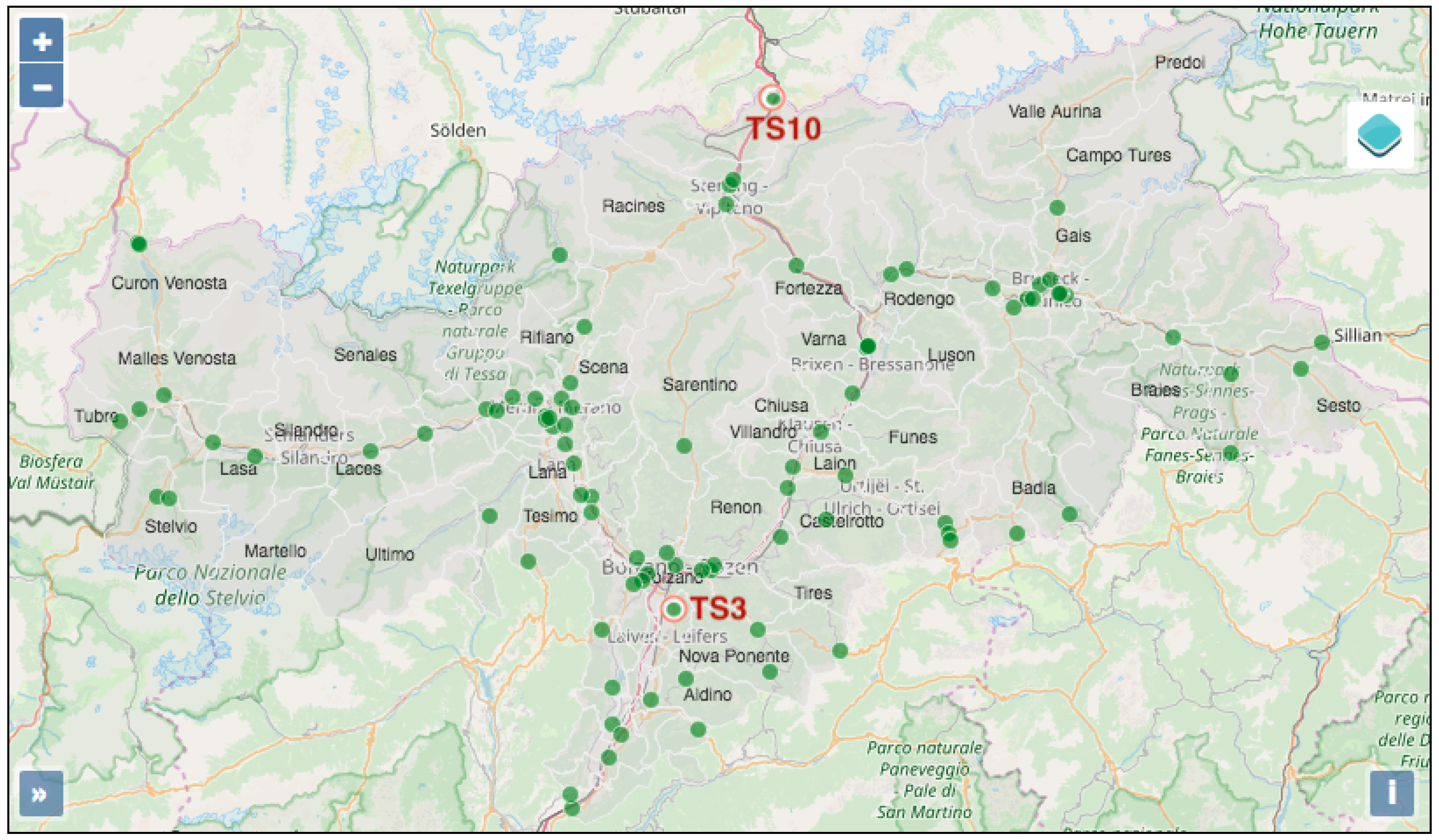
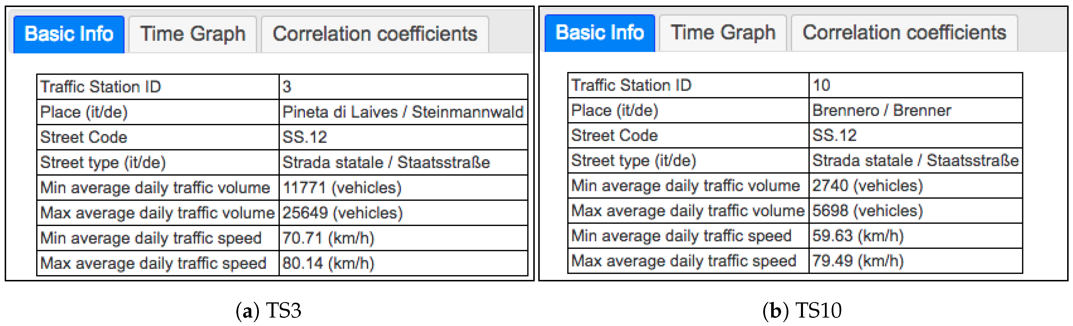
As a demonstration of the system, we select for the analysis two months of data of January and July 2017. More specifically, we focus on the analysis of three types of observations: precipitation, traffic volume, and traffic speed. We choose the two traffic stations TS3 and TS10 (respectively with ID 3 and ID 10) for illustration, where TS3 is located near the capital city Bolzano of South Tyrol, and TS10 is located in the north of the province and close to the border to Austria. Figure 7 shows the locations of these two stations. Below we analyze the spatial and temporal patterns of the observations, and their correlations.
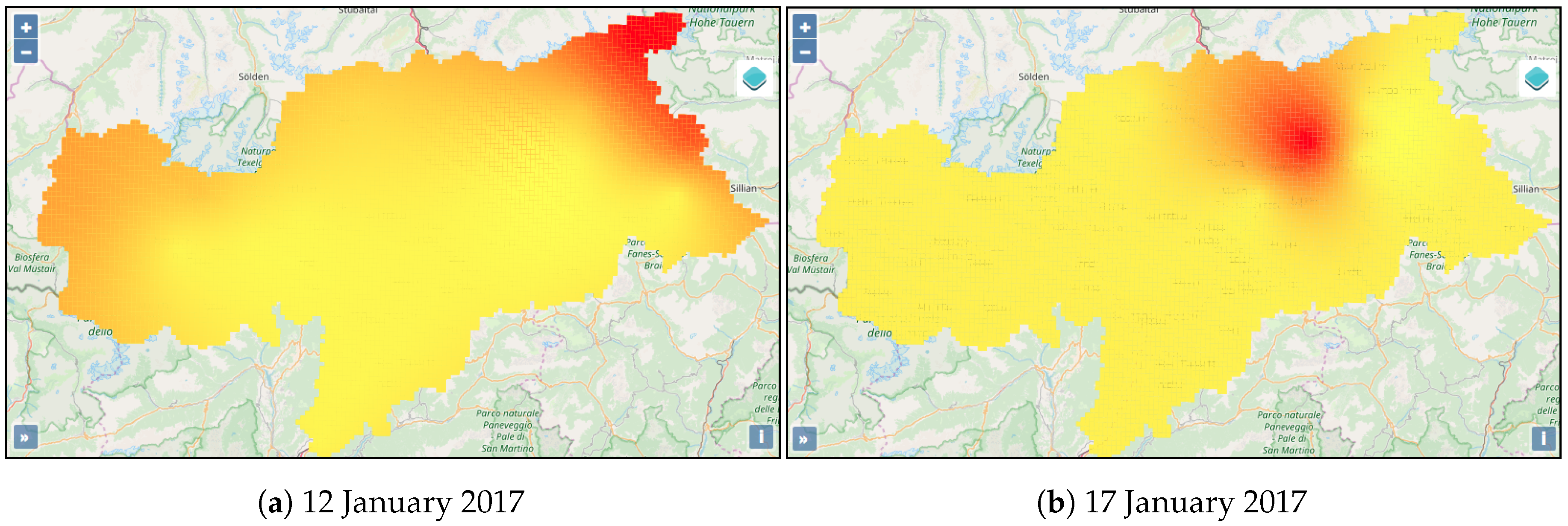
Spatial patterns. The basic information of TS3 and TS10 and their aggregated statistical values are shown in Figure 8. TS3 and TS10 are located in the regions of “Pineta di Laives” and “Brennero” respectively, and at two road segments of the national-level street with the code SS.12. We first examine the traffic volume and speed at these two stations. In January, for the traffic volume, TS3 is much “busier” than TS10, according to both the average min and max and values. For daily average traffic speed, the min value at ST3 is higher than that at TS10, while the max speeds at TS3 and TS10 are similar, due to the speed limit. The precipitation distribution varies strongly at different locations and days. Figure 9 shows precipitation interpolated on the grid cells on the 12 and 17 January 2017, with precipitation hotspots located in different areas.
Temporal patterns. We use 2-D scatter plots and line plots to show the temporal variations of the multivariate. Figure 10 shows the values of precipitation, traffic speed, and volume in January and July 2017 at TS3. As expected, the precipitation in July is significantly higher than in January. Moreover precipitation varies dramatically in both months. For traffic speed and volume, there is an obvious negative correlation. We also observe a clear weekly pattern that traffic volumes are larger in weekdays and smaller at weekends, but the speeds exhibit an opposite pattern. In general, the traffic volume is larger in July than in January, but the traffic speeds are similar in January and July.
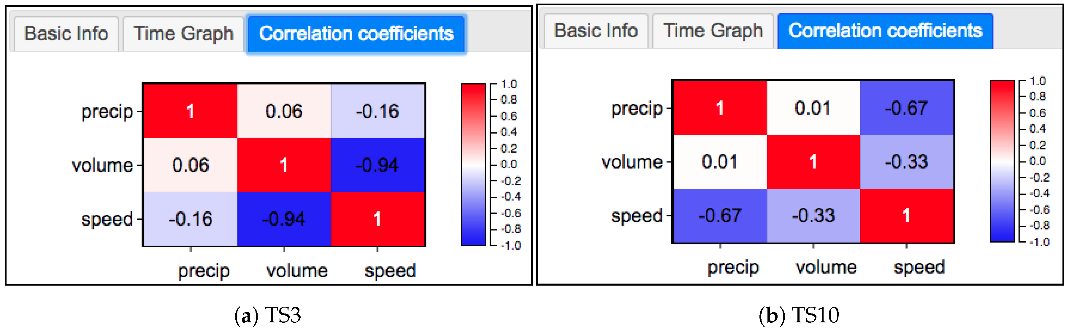
Correlation of observations. We use a correlation coefficient matrix to show the correlations () among multiple variables. Figure 11 shows the correlation coefficient matrices of TS3 and TS10 in January 2017. From the figures, we can see that in general there is no linear correlation (∼0) between precipitation and volume at both TS3 () and TS10 (), while precipitation has a negative correlation with traffic speed, and the correlation is more significant at TS10 () than at TS3 (). The traffic volume and speed have an obvious negative correlation, and at TS3 it is very strong ().
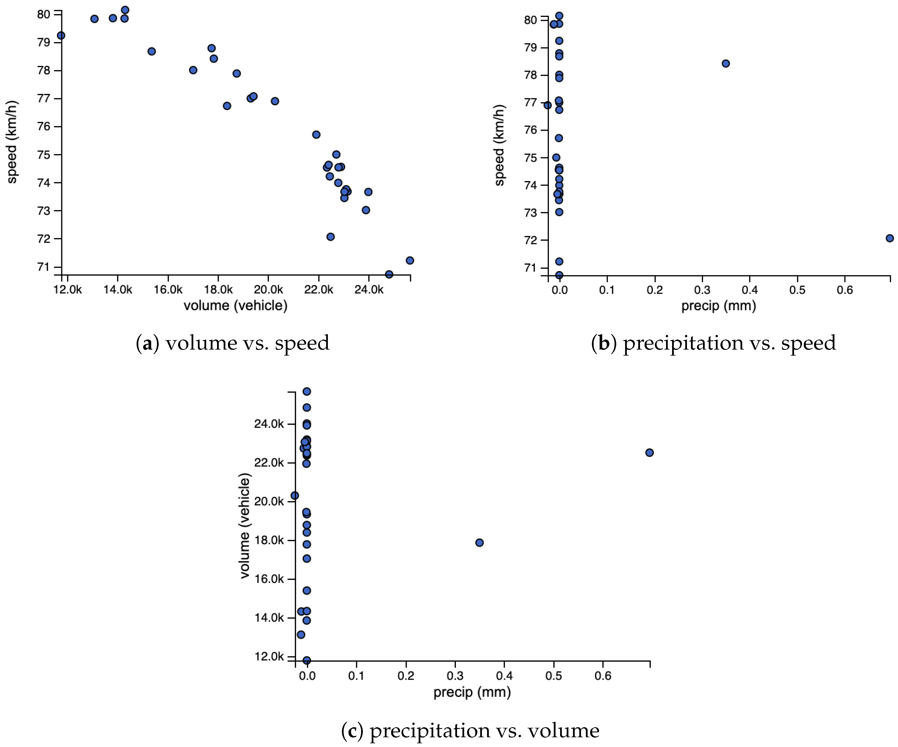
Furthermore, users can interactively explore the details of the correlations between two variables by clicking a specific cell in the matrix. Figure 12 displays the three bivariate plots at TS3 in January 2017. Figure 12a shows a very clear negative linear correlation between volume and speed, while Figure 12b,c show no linear correlation, as the points are mostly scattered around the vertical axis.
4.5. Preliminary Studies
We have carried out an evaluation of the framework with respect to its appropriateness in supporting the formulation of sensor data analysis tasks through the visual interface, the formulation of the SPARQL queries, and in reducing the complexity from SPARQL to SQL. In addition, we have collected general feedback from various stakeholders.
4.5.1. Exploring Effectiveness
We measure the effectiveness by verifying whether typical sensor data analysis tasks and queries can be expressed over the visual interface and the ontologies that we developed. Below, we consider three tasks that can be done from the graphical user interface. We show the SPARQL queries generated by the interface and their graphical representations. In addition, we explain the SQL queries. Below we present three of these tasks, formulating them in natural language, in SPARQL, in the corresponding graphic representation and in SQL. The tasks and queries are presented in increasing complexity.
Task 1: “Get all the sensors and their locations.” This task can be executed with just one click on the “Stations” checkbox in the visual interface. The corresponding SPARQL query and its graphical representation visualized on the interface are:

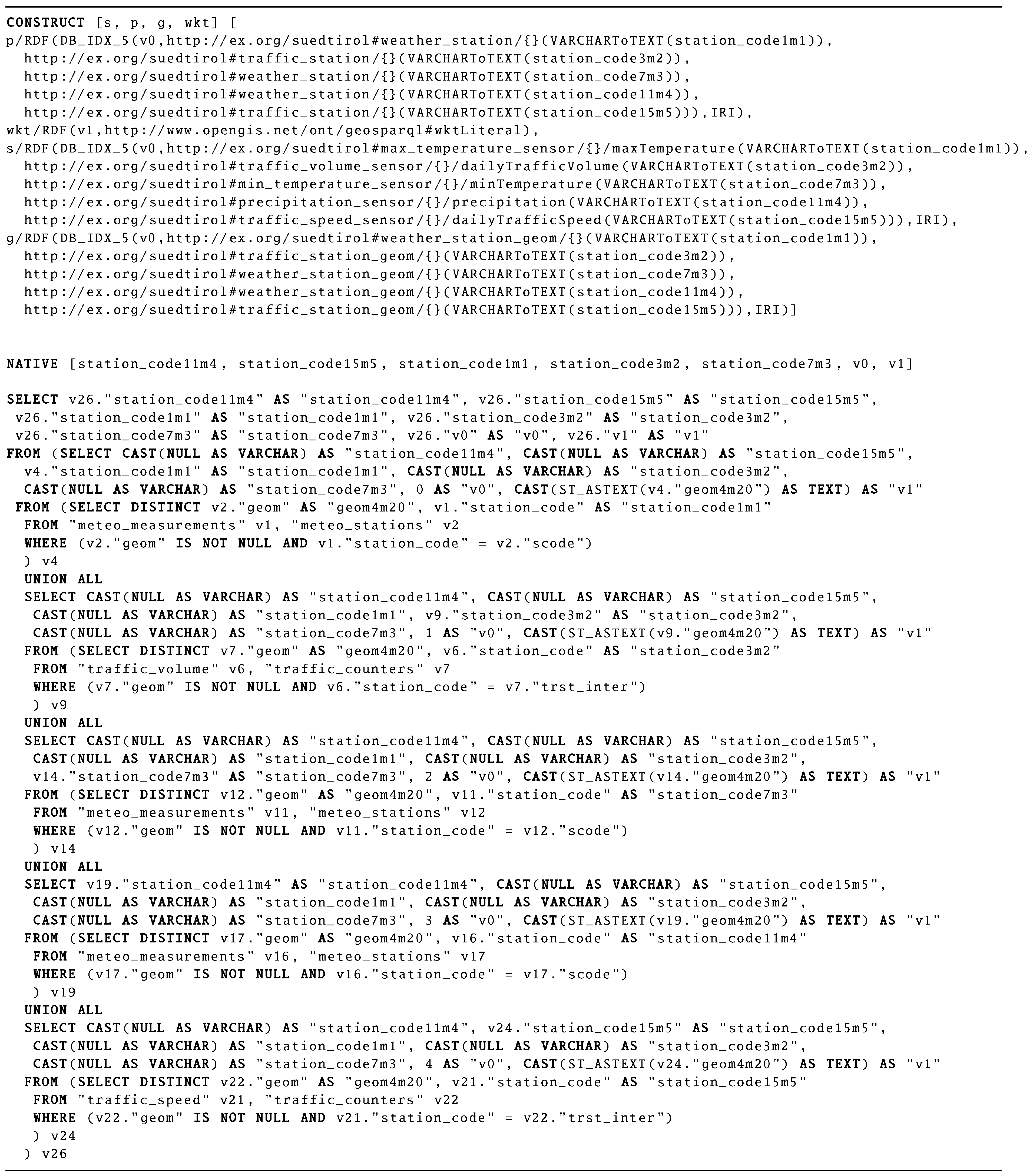
This SPARQL query only uses vocabularies from the SOSA and GeoSPARQL ontologies, and is very easy to understand. As shown in Figure 13, Ontop translates the SPARQL query to a SQL query (starting with the line NATIVE) to be evaluated over the database, together with a post-processing step (starting with the line CONSTRUCT) to construct the SPARQL answers. The SQL query is a union of 5 subqueries, and each subquery is a join of two tables. We remark that the generated SQL query is actually optimal in the sense that its structure is very close to the one produced by human experts. Hence, compared with the SPARQL counterpart, the SQL query is much more difficult to understand and to write manually.
Task 2: “Get all the sensors, their locations, and observations on 1 January 2017.” This is done by one more click using the time selection function in the interface. The corresponding SPARQL query and its graphical representation are:

The generated SQL query, which we do not include here for space reasons, has a similar structure as the one for Task 1, but projects more columns and uses more filter conditions for the selected time period.
Task 3: “Get all the sensors, their locations, and observations in the municipality of Bolzano on 1 January 2017.” This is done by one more click on the map over the municipality of “Bolzano” in the interface. Compared with the SQL query generated for Task 2, now each sub-query needs to join with another table of the municipality using a spatial filter. For space reasons, we do not include the generated query here, and just observe that the gap between the SPARQL query and the SQL query becomes even more significant than in the previous tasks.

Overall, this evaluation shows that (1) to collect information for analysis, the user interface can generate SPARQL queries that are easy to understand; (2) the corresponding SQL query is much more involved, and would be difficult to write and understand by a human expert. This confirms that our approach can effectively support users to get information for performing their analysis tasks.
4.5.2. Feedback
The GOdIVA framework was first presented at the 9th Workshop of “Computer Science Research Meets Business” on GIS and Location-based Services, held on 23 November 2017 (https://www.unibz.it/en/events/126513), organized by the Free University of Bozen-Bolzano (unibz). Among the attendants, were (1) Südtiroler Informatik AG (SIAG) (https://www.siag.it/de/home/), who is managing the OpenDataPortal, (2) ASTAT, who is in charge of the local traffic data, (3) NOI Techpark (https://noi.bz.it/en/), a local service provider for companies, and (4) R3 GIS (https://www.r3-gis.com/en/), an SME specialized in the development of GIS technology. The feedback from the attendants was very positive and they showed strong interest in adopting this approach to integrate and analyze their data sources. They were particularly happy to see that data coming from different providers and in different formats could be integrated and visualized. Since then, several follow-up meetings, including dedicated demos and a hackthon to play with further data sources, were held with these stakeholders, with the aim of defining concrete collaborations. In the end, these activities have directly triggered two large industrial projects on geodata integration and analysis, where the GOdIVA framework is used as the core technology.
- IDEE: Data Integration for Energy Efficiency (https://ideenergy.eu/) is a 3-year project supported by European Regional Development Fund (ERDF). The aim of the IDEE project is to develop a technological infrastructure based on semantic technologies for the integration of data concerning buildings, with an emphasis on the energy related data, and to provide techniques and tools for the visualization and analysis of such data. The consortium consists of unibz (geodata integration solution provider), Alperia (energy consumption data provider), and R3 GIS (GIS infrastructure provider), and has the city of Merano as the main use-case partner providing both requirements and data about the city.
- Open Data Hub-Virtual Knowledge Graph is a joint project between NOI techpark and Ontopic (http://ontopic.biz/) to extend the South Tyrolean OpenDataHub (https://opendatahub.bz.it/) with a Knowledge Graph interface (https://sparql.opendatahub.bz.it/). The first phase to integrate tourism data (e.g., about hotels and events) is already completed, and a second phase with the aim of integrating traffic data has started. In addition, following the principle of GOdIVA, we have created a Web Component (https://webcomponents.opendatahub.bz.it/webcomponent/567cb2e2-3e5d-421a-bf85-b8ecc500aab9), which can be embedded into any web page like a standard HTML tag, to visualize SPARQL query results in different ways, including customized maps.
5. Conclusions and Future Work
In this paper, we discussed several challenges in integrating and analyzing heterogeneous geospatial data. We address these challenges by proposing a framework, called GOdIVA, uniting the two well-established research areas of ontology-based data integration and geovisual analytics, by placing an ontology at the center. In GOdIVA, the ontology-based integration module aims at providing an interoperable and manageable geodata infrastructure for heterogeneous data sources, whereas the geovisual analytics module exploits the structure of the ontology and delivers diverse but easily comprehensible visual expressions for understanding and exploration. To test our approach, we implemented a web-based visual analytical system, and used heterogeneous sensor observations collected in the province of South Tyrol, Italy as test data. A preliminary evaluation has been conducted and two follow-up industrial projects were briefly presented. The experiment confirmed our hypothesis that GOdIVA framework is feasible for the exploration and understanding heterogeneous geospatial data.
Future Work. In this paper, we used historical sensor data for one year as a demonstration. We plan to investigate longer-term time series data for further spatiotemporal analysis to discover long-term trends and periodic patterns. We will also include data from other domains into our study. Moreover, we consider processing real-time sensor data streams in our future work.
For the purpose of interoperability, we have used several standard ontologies. In the future, we plan to adopt more standards, in particular, we are interested in QB4ST (https://www.w3.org/TR/qb4st/) from Spatial Data on the Web Working Group, an extension of the RDF Data Cube Vocabulary (https://www.w3.org/TR/vocab-data-cube/) for spatiotemporal components. Another promising direction is to integrate cityGML data for digital 3D models of cities and landscapes [79]. The semantics of the SPARQL query [80] to support the mapping can be further explored construction, making sure the we get desired answers.
Regarding the GeoVA module, there are several aspects we can improve. First, we will enrich the data access view so that it can be generated following the common access patterns of the ontology, and users can combine these patterns to form more complex queries. For example, information dashboard design strategies can be adopted to improve the visual interface [81]. In addition, we will propose more appropriate visualization techniques, e.g., by incorporating scientific visualization and thematic mappings techniques to achieve synergetic effects [75]. Currently, we implemented some aggregation and correlation coefficient functionalities for demonstration purposes. Further spatial statistics and machine learning algorithms will be integrated for spatiotemporal analysis. Overall, we will provide additional functionalities to automatically generate substantial parts of the user interface, we will provide more analysis functions, and overall we will make the GeoVA module more user friendly.
References yes
Author Contributions
Conceptualization: Linfang Ding, Guohui Xiao, Diego Calvanese, and Liqiu Meng; methodology: Linfang Ding and Guohui Xiao; project administration: Diego Calvanese and Liqiu Meng; software: Linfang Ding and Guohui Xiao; visualization: Linfang Ding; writing—original draft: Linfang Ding and Guohui Xiao; writing—review and editing: Diego Calvanese and Liqiu Meng. All authors have read and agreed to the published version of the manuscript.
Funding
This research has been partially supported by the EU H2020 project INODE, by the Italian PRIN project HOPE, by the European Regional Development Fund (ERDF) Investment for Growth and Jobs Programme 2014-2020 through the project IDEE (FESR1133), by the Free University of Bozen-Bolzano through the projects QUADRO, KGID, and GeoVKG, by the Jiangsu Industrial Technology Research Institute (JITRI), by the Changshu Fengfan Power Equipment Co., Ltd., and by the Wallenberg AI, Autonomous Systems and Software Program (WASP) funded by the Knut and Alice Wallenberg Foundation.
Conflicts of Interest
The authors declare no conflict of interest.
References
- Thomas, J.J.; Cook, K.A. A visual analytics agenda. IEEE Comput. Graph. Appl. 2006, 26, 10–13. [Google Scholar] [CrossRef]
- Keim, D.A.; Kohlhammer, J.; Ellis, G.; Mansmann, F. (Eds.) Mastering the Information Age-Solving Problems with Visual Analytics; Eurographics Association: Goslar, Germany, 2010. [Google Scholar]
- Robinson, A.C.; Demšar, U.; Moore, A.B.; Buckley, A.; Jiang, B.; Field, K.; Kraak, M.J.; Camboim, S.P.; Sluter, C.R. Geospatial big data and cartography: Research challenges and opportunities for making maps that matter. Int. J. Cartogr. 2017, 3, 32–60. [Google Scholar] [CrossRef] [Green Version]
- Kuhn, W. Core concepts of spatial information for transdisciplinary research. Int. J. Geogr. Inf. Sci. 2012, 26, 2267–2276. [Google Scholar] [CrossRef]
- Kharlamov, E.; Hovland, D.; Skjæveland, M.G.; Bilidas, D.; Jiménez-Ruiz, E.; Xiao, G.; Soylu, A.; Lanti, D.; Rezk, M.; Zheleznyakov, D.; et al. Ontology based data access in Statoil. J. Web Semant. 2017, 44, 3–36. [Google Scholar] [CrossRef] [Green Version]
- Xiao, G.; Calvanese, D.; Kontchakov, R.; Lembo, D.; Poggi, A.; Rosati, R.; Zakharyaschev, M. Ontology-Based Data Access: A survey. In Proceedings of the 27th International Joint Conference on Artificial Intelligence (IJCAI), IJCAI Org, Stockholm, Sweden, 13–19 July 2018; pp. 5511–5519. [Google Scholar]
- Perry, M.; Herring, J. GeoSPARQL-A Geographic Query Language for RDF Data; OGC Candidate Standard OGC 11-052r3; Open Geospatial Consortium: Wayland, MA, USA, 2011. [Google Scholar]
- Cox, S.; Little, C. Time ontology in OWL; W3C Recommendation, W3C: Cambridge, MA, USA, 2017. [Google Scholar]
- Haller, A.; Janowicz, K.; Cox, S.; Phuoc, D.L.; Taylor, K.; Lefrançois, M. Semantic Sensor Network Ontology; W3C recommendation, W3C: Cambridge, MA, USA, 2017. [Google Scholar]
- Calvanese, D.; Cogrel, B.; Komla-Ebri, S.; Kontchakov, R.; Lanti, D.; Rezk, M.; Rodriguez-Muro, M.; Xiao, G. Ontop: Answering SPARQL queries over relational databases. Semant. Web J. 2017, 8, 471–487. [Google Scholar] [CrossRef] [Green Version]
- Vaccari, L.; Shvaiko, P.; Marchese, M. A geo-service semantic integration in spatial data infrastructures. Int. J. Spat. Data Infrastruc. Res. 2009, 4, 24–51. [Google Scholar]
- Meng, L. From multiple geodata sources to diverse maps. In Frontiers in Geoinformations; Lin, H., Shi, X., Eds.; Higher Education Press: Beijing, China, 2017; Chapter 11; pp. 191–218. [Google Scholar]
- Harvey, F.; Kuhn, W.; Pundt, H.; Bishr, Y.; Riedemann, C. Semantic interoperability: A central issue for sharing geographic information. Ann. Reg. Sci. 1999, 33, 213–232. [Google Scholar] [CrossRef]
- Hong, J.H.; Kuo, C.L. A semi-automatic lightweight ontology bridging for the semantic integration of cross-domain geospatial information. Int. J. Geogr. Inf. Sci. 2015, 29, 2223–2247. [Google Scholar] [CrossRef]
- Manola, F.; Mille, E. RDF Primer. W3C Recommendation, W3C, 2004. Available online: https://www.w3.org/TR/rdf-primer/ (accessed on 27 July 2020).
- Hitzler, P.; Krötzsch, M.; Parsia, B.; Patel-Schneider, P.F.; Rudolph, S. OWL 2 Web Ontology Language: Primer (Second Edition). W3C Recommendation, W3C, 2012. Available online: http://www.w3.org/TR/owl2-primer/ (accessed on 27 July 2020).
- Wu, Y.; Moylan, E.; Inman, H.; Graf, C. Paving the Way to Open Data. Data Intell. 2019, 1, 368–380. [Google Scholar] [CrossRef]
- Hakimpour, F.; Timpf, S. Using ontologies for resolution of semantic heterogeneity in GIS. In Proceedings of the 4th AGILE Conference on Geographic Information Science, Olhao, Portugal, 19 April 2001; pp. 385–395. [Google Scholar]
- Bittner, T.; Donnelly, M.; Smith, B. A spatio-temporal ontology for geographic information integration. Int. J. Geogr. Inf. Sci. 2009, 23, 765–798. [Google Scholar] [CrossRef] [Green Version]
- Zhang, C.; Zhao, T.; Li, W.; Osleeb, J.P. Towards logic-based geospatial feature discovery and integration using web feature service and geospatial semantic web. Int. J. Geogr. Inf. Sci. 2010, 24, 903–923. [Google Scholar] [CrossRef]
- Hu, Y.; Janowicz, K.; Carral, D.; Scheider, S.; Kuhn, W.; Berg-Cross, G.; Hitzler, P.; Dean, M.; Kolas, D. A geo-ontology design pattern for semantic trajectories. In Spatial Information Theory; Tenbrink, T., Stell, J., Galton, A., Wood, Z., Eds.; Springer: Berlin/Heidelberg, Germany, 2013; pp. 438–456. [Google Scholar]
- Xu, J.; Nyerges, T.L.; Nie, G. Modeling and representation for earthquake emergency response knowledge: Perspective for working with geo-ontology. Int. J. Geogr. Inf. Sci. 2014, 28, 185–205. [Google Scholar] [CrossRef]
- Jiang, Y.; Li, Y.; Yang, C.; Liu, K.; Armstrong, E.M.; Huang, T.; Moroni, D.F.; Finch, C.J. A comprehensive methodology for discovering semantic relationships among geospatial vocabularies using oceanographic data discovery as an example. Int. J. Geogr. Inf. Sci. 2017, 31, 2310–2328. [Google Scholar] [CrossRef]
- Chen, N.; Chen, Z.; Hu, C.; Di, L. A capability matching and ontology reasoning method for high precision OGC web service discovery. Int. J. Digit. Earth 2011, 4, 449–470. [Google Scholar] [CrossRef]
- Li, W.; Goodchild, M.F.; Raskin, R. Towards geospatial semantic search: Exploiting latent semantic relations in geospatial data. Int. J. Digit. Earth 2014, 7, 17–37. [Google Scholar] [CrossRef]
- Hahmann, T.; Stephen, S. Using a hydro-reference ontology to provide improved computer-interpretable semantics for the groundwater markup language (GWML2). Int. J. Geogr. Inf. Sci. 2018, 32, 1138–1171. [Google Scholar] [CrossRef]
- Poggi, A.; Lembo, D.; Calvanese, D.; De Giacomo, G.; Lenzerini, M.; Rosati, R. Linking data to ontologies. J. Data Semant. 2008, 10, 133–173. [Google Scholar] [CrossRef]
- Das, S.; Sundara, S.; Cyganiak, R. R2RML: RDB to RDF Mapping Language. W3C Recommendation, W3C, 2012. Available online: http://www.w3.org/TR/r2rml/ (accessed on 27 July 2020).
- Xiao, G.; Hovland, D.; Bilidas, D.; Rezk, M.; Giese, M.; Calvanese, D. Efficient ontology-based data integration with canonical IRIs. In Lecture Notes in Computer Science, Proceedings of the 15th Extended Semantic Web Conference (ESWC), Heraklion, Crete, Greece, 3–7 June 2018; Springer: Berlin/Heidelberg, Germany, 2018; Volume 10843, pp. 697–713. [Google Scholar] [CrossRef]
- Calvanese, D.; De Giacomo, G.; Lembo, D.; Lenzerini, M.; Poggi, A.; Rodriguez-Muro, M.; Rosati, R.; Ruzzi, M.; Savo, D.F. The Mastro system for ontology-based data access. Semant. Web J. 2011, 2, 43–53. [Google Scholar] [CrossRef] [Green Version]
- Priyatna, F.; Corcho, O.; Sequeda, J.F. Formalisation and experiences of R2RML-based SPARQL to SQL query translation using morph. In Proceedings of the 23rd International Conference on World Wide Web, Seoul, Korea, 7–11 April 2014; pp. 479–490. [Google Scholar] [CrossRef]
- Sequeda, J.F.; Miranker, D.P. Ultrawrap: SPARQL execution on relational data. J. Web Semant. 2013, 22, 19–39. [Google Scholar] [CrossRef] [Green Version]
- Bereta, K.; Xiao, G.; Koubarakis, M. Ontop-spatial: Ontop of geospatial databases. J. Web Semant. 2019, 58. [Google Scholar] [CrossRef]
- Stadler, C.; Lehmann, J.; Höffner, K.; Auer, S. LinkedGeoData: A core for a web of spatial open data. Semant. Web J. 2012, 3, 333–354. [Google Scholar] [CrossRef]
- Xiao, G.; Ding, L.; Cogrel, B.; Calvanese, D. Virtual Knowledge Graphs: An overview of systems and use cases. Data Intell. 2019, 1, 201–223. [Google Scholar] [CrossRef]
- Ding, L.; Xiao, G.; Calvanese, D.; Meng, L. Consistency assessment for open geodata integration: An ontology-based approach. Geoinformatica 2019. [Google Scholar] [CrossRef]
- Brüggemann, S.; Bereta, K.; Xiao, G.; Koubarakis, M. Ontology-based Data Access for maritime security. In Lecture Notes in Computer Science, Proceedings of the 13th Extended Semantic Web Conference (ESWC), Crete, Greece, May 29–June 2 2016; Springer: Berlin/Heidelberg, Germany, 2016; Volume 9678, pp. 741–757. [Google Scholar]
- Robinson, A. Geovisual analytics. Geogr. Inf. Sci. Technol. Body Knowl. 2017, 2017. [Google Scholar] [CrossRef]
- Andrienko, G.; Andrienko, N.; Keim, D.; MacEachren, A.M.; Wrobel, S. Challenging problems of geospatial visual analytics. J. Vis. Lang. Comput. 2011, 22, 251–256. [Google Scholar] [CrossRef]
- Andrienko, G.; Andrienko, N.; Bak, P.; Keim, D.; Wrobel, S. Visual Analytics of Movement; Springer: Berlin/Heidelberg, Germany, 2013. [Google Scholar]
- Ding, L.; Fan, H.; Meng, L. Understanding taxi driving behaviors from movement data. In Lecture Notes in Geoinformation and Cartography; Springer: Berlin/Heidelberg, Germany, 2015; pp. 219–234. [Google Scholar]
- Ding, L.; Krisp, J.M.; Meng, L. Visual analysis of floating car data. In Geospatial Data Science Techniques and Applications; Karimi, H.A., Karimi, B., Eds.; CRC Press: Boca Raton, FL, USA, 2017. [Google Scholar]
- Pezanowski, S.; MacEachren, A.M.; Savelyev, A.; Robinson, A.C. SensePlace3: A geovisual framework to analyze place–time–attribute information in social media. Cartogr. Geogr. Inf. Sci. 2018, 45, 420–437. [Google Scholar] [CrossRef]
- Zhu, R.; Lin, D.; Jendryke, M.; Zuo, C.; Ding, L.; Meng, L. Geo-tagged social media data-based analytical approach for perceiving impacts of social events. ISPRS Int. J. Geo-Inf. 2018, 8, 15. [Google Scholar] [CrossRef] [Green Version]
- Sibolla, B.H.; Coetzee, S.; Van Zyl, T.L. A framework for visual analytics of spatio-temporal sensor observations from data streams. ISPRS Int. J. Geo-Inf. 2018, 7, 475. [Google Scholar] [CrossRef] [Green Version]
- Andrienko, G.; Andrienko, N.; Jankowski, P.; Keim, D.; Kraak, M.; MacEachren, A.; Wrobel, S. Geovisual analytics for spatial decision support: Setting the research agenda. Int. J. Geogr. Inf. Sci. 2007, 21, 839–857. [Google Scholar] [CrossRef]
- Janowicz, K.; Schade, S.; Bröring, A.; Keßler, C.; Maué, P.; Stasch, C. Semantic enablement for spatial data infrastructures. Trans. GIS 2010, 14, 111–129. [Google Scholar] [CrossRef]
- Wang, X.; Jeong, D.H.; Dou, W.; Lee, S.W.; Ribarsky, W.; Chang, R. Defining and applying knowledge conversion processes to a visual analytics system. Comput. Graph. 2009, 33, 616–623. [Google Scholar] [CrossRef] [Green Version]
- Vatin, G.; Napoli, A. Using ontologies for proposing adequate geovisual analytics solutions in the analysis of trajectories. In Proceedings of the 18th International Conference on Information Visualisation, Paris, France, 16–18 July 2014; pp. 176–182. [Google Scholar] [CrossRef] [Green Version]
- Katifori, A.; Halatsis, C.; Lepouras, G.; Vassilakis, C.; Giannopoulou, E. Ontology visualization methods—A survey. ACM Comput. Surv. 2007, 39, 10. [Google Scholar] [CrossRef] [Green Version]
- Lutz, M.; Klien, E. Ontology-based retrieval of geographic information. Int. J. Geogr. Inf. Sci. 2006, 20, 233–260. [Google Scholar] [CrossRef]
- Soylu, A.; Kharlamov, E.; Zheleznyakov, D.; Jiménez-Ruiz, E.; Giese, M.; Skjæveland, M.G.; Hovland, D.; Schlatte, R.; Brandt, S.; Lie, H.; et al. OptiqueVQS: A visual query system over ontologies for industry. Semant. Web J. 2018, 9, 627–660. [Google Scholar] [CrossRef] [Green Version]
- Beek, W.; Folmer, E.; Rietveld, L.; Walker, J. GeoYASGUI: The GeoSPARQL query editor and result set visualizer. ISPRS Int. Arch. Photogramm. Remote Sens. Spat. Inf. Sci. 2017, XLII-4/W2, 39–42. [Google Scholar] [CrossRef] [Green Version]
- Nikolaou, C.; Dogani, K.; Bereta, K.; Garbis, G.; Karpathiotakis, M.; Kyzirakos, K.; Koubarakis, M. Sextant: Visualizing time-evolving linked geospatial data. J. Web Semant. 2015, 35, 35–52. [Google Scholar] [CrossRef] [Green Version]
- Scheider, S.; Degbelo, A.; Lemmens, R.; van Elzakker, C.; Zimmerhof, P.; Kostic, N.; Jones, J.; Banhatti, G. Exploratory querying of SPARQL endpoints in space and time. Semant. Web J. 2017, 8, 65–86. [Google Scholar] [CrossRef]
- Brasoveanu, A.M.P.; Sabou, M.; Scharl, A.; Hubmann-Haidvogel, A.; Fischl, D. Visualizing statistical linked knowledge for decision support. Semant. Web J. 2017, 8, 113–137. [Google Scholar] [CrossRef] [Green Version]
- Huang, W.; Harrie, L. Towards knowledge-based geovisualisation using Semantic Web technologies: A knowledge representation approach coupling ontologies and rules. Int. J. of Digital Earth 2019, 1–22. [Google Scholar] [CrossRef] [Green Version]
- Dadzie, A.S.; Pietriga, E. Visualisation of linked data—Reprise. Semant. Web J. 2017, 8, 1–21. [Google Scholar] [CrossRef] [Green Version]
- Muller, C.L.; Chapman, L.; Grimmond, C.S.B.; Young, D.T.; Cai, X. Sensors and the city: A review of urban meteorological networks. Int. J. Climatol. 2013, 33, 1585–1600. [Google Scholar] [CrossRef]
- Jaroszweski, D.; McNamara, T. The influence of rainfall on road accidents in urban areas: A weather radar approach. Travel Behav. Soc. 2014, 1, 15–21. [Google Scholar] [CrossRef] [Green Version]
- Bijleveld, F.; Churchill, T. The Influence of Weather Conditions on Road Safety: An Assessment of the Effect of Precipitation and Temperature; Leidschendam, SWOV Institute for Road Safety Research: Hague, The Netherlands, 2009. [Google Scholar]
- Kwak, H.Y.; Ko, J.; Lee, S.; Joh, C.H. Identifying the correlation between rainfall, traffic flow performance and air pollution concentration in Seoul using a path analysis. Transp. Res. Procedia 2017, 25, 3552–3563. [Google Scholar] [CrossRef]
- Llaves, A.; Kuhn, W. An event abstraction layer for the integration of geosensor data. Int. J. Geogr. Inf. Sci. 2014, 28, 1085–1106. [Google Scholar] [CrossRef] [Green Version]
- Devaraju, A.; Kuhn, W.; Renschler, C.S. A formal model to infer geographic events from sensor observations. Int. J. Geogr. Inf. Sci. 2015, 29, 1–27. [Google Scholar] [CrossRef] [Green Version]
- Dell’Aglio, D.; Della Valle, E.; van Harmelen, F.; Bernstein, A. Stream reasoning: A survey and outlook. Data Sci. 2017, 1, 59–83. [Google Scholar] [CrossRef] [Green Version]
- Barbieri, D.F.; Braga, D.; Ceri, S.; Della Valle, E.; Grossniklaus, M. Querying RDF streams with C-SPARQL. SIGMOD Rec. 2010, 39, 20–26. [Google Scholar] [CrossRef]
- Phuoc, D.L.; Dao-Tran, M.; Parreira, J.X.; Hauswirth, M. A native and adaptive approach for unified processing of linked streams and linked data. In Proceedings of the 10th International Semantic Web Conference (ISWC), Part 1, Bonn, Germany, 23–27 October 2011; pp. 370–388. [Google Scholar] [CrossRef]
- Dell’Aglio, D.; Della Valle, E.; Calbimonte, J.P.; Corcho, Ó. RSP-QL Semantics: A Unifying Query Model to Explain Heterogeneity of RDF Stream Processing Systems. Int. J. Semant. Web Inf. Syst. 2014, 10, 17–44. [Google Scholar] [CrossRef]
- Brandt, S.; Güzel Kalaycı, E.; Ryzhikov, V.; Xiao, G.; Zakharyaschev, M. Querying log data with Metric Temporal Logic. J. Artif. Intell. Res. 2018, 62, 829–877. [Google Scholar]
- Motik, B.; Cuenca Grau, B.; Horrocks, I.; Wu, Z.; Fokoue, A.; Lutz, C. OWL 2 Web Ontology Language Profiles (Second Edition). W3C Recommendation, W3C, 2012. Available online: http://www.w3.org/TR/owl2-profiles/ (accessed on 27 July 2020).
- Brickley, D.; Guha, R. RDF Schema 1.1. W3C Recommendation, W3C, 2014. Available online: https://www.w3.org/TR/rdf-schema/ (accessed on 27 July 2020).
- Harris, S.; Seaborne, A. SPARQL 1.1 Query Language. W3C Recommendation, W3C, 2013. Available online: http://www.w3.org/TR/sparql11-query (accessed on 27 July 2020).
- Feigenbaum, L.; Williams, G.T.; Clark, K.G.; Torres, E. SPARQL 1.1 Protocol. W3C Recommendation, W3C, 2013. Available online: http://www.w3.org/TR/sparql11-protocol (accessed on 27 July 2020).
- Scheider, S.; Tomko, M. Knowing whether spatio-temporal analysis procedures are applicable to datasets. In Formal Ontology in Information Systems; Frontiers in Artificial Intelligence and Applications; Ferrario, R., Werner, K., Eds.; IOS Press: Amsterdam, The Netherlands, 2016. [Google Scholar]
- Ding, L.; Meng, L. A comparative study of thematic mapping and scientific visualization. Ann. GIS 2014, 20, 23–37. [Google Scholar] [CrossRef]
- Worboys, M. Event-oriented approaches to geographic phenomena. Int. J. Geogr. Inf. Sci. 2005, 19, 1–28. [Google Scholar] [CrossRef]
- Gennari, J.H.; Musen, M.A.; Fergerson, R.W.; Grosso, W.E.; Crubézy, M.; Eriksson, H.; Fridman Noy, N.; Tu, S.W. The evolution of Protégé: An environment for knowledge-based systems development. Int. J. Hum.-Comput. Stud. 2003, 58, 89–123. [Google Scholar] [CrossRef]
- Hake, G.; Grünreich, D.; Meng, L. Kartographie: Visualisierung raum-zeitlicher Informationen; Walter de Gruyter: Berlin, Germany, 2013. [Google Scholar]
- Gröger, G.; Kolbe, T.H.; Nagel, C.; Häfele, K.H. OGC City Geography Markup Language (CityGML) Encoding standard; OpenGIS Encoding Standard OGC 12-019; Open Geospatial Consortium: Wayland, MA, USA, 2012. [Google Scholar]
- Zhang, X.; den Bussche, J.V.; Picalausa, F. On the satisfiability problem for SPARQL patterns. J. Artif. Intell. Res. 2016, 56, 403–428. [Google Scholar]
- Few, S. Information Dashboard Design: The Effective Visual Communication of Data; O’Reilly Media, Inc.: Sebastopol, CA, USA, 2006. [Google Scholar]
Figure 1.
The Ontology-based Geodata Integration for Geovisual Analytics (GOdIVA) framework.

Figure 2.
The province of South Tyrol.

Figure 3.
The partition of the study area into grid cells and the interpolation result.

Figure 4.
A fragment of the ontology.

Figure 5.
Example triples generated by the mapping assertions.

Figure 6.
The visual interface.

Figure 7.
The locations of traffic stations with TS3 and TS10 being highlighted.

Figure 8.
The basic information of selected traffic stations in January 2017.

Figure 9.
A heat map showing the distribution of precipitation.

Figure 10.
Diagrams of time series at TS3 for precipitation, traffic speed, and volume.
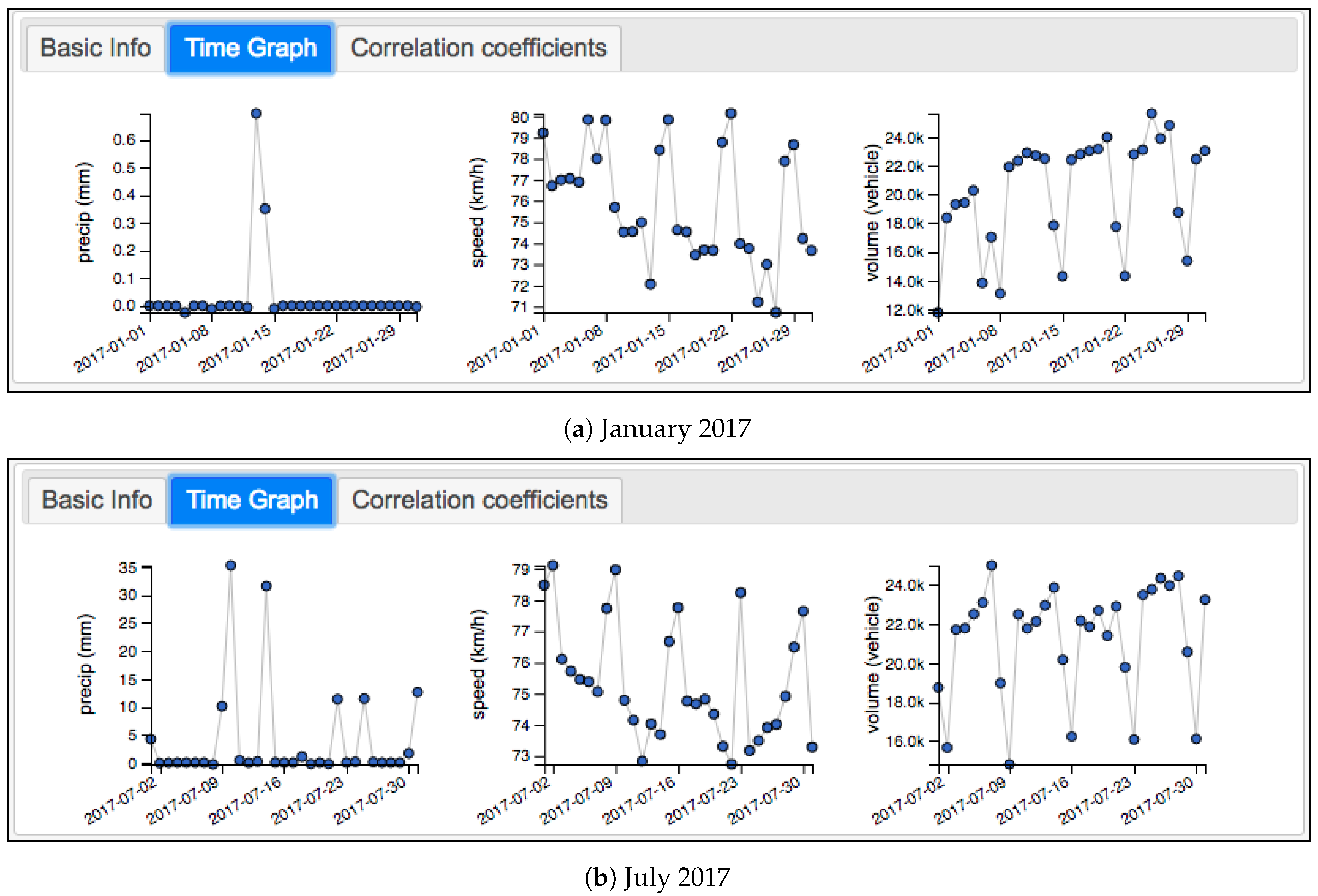
Figure 11.
Correlation coefficient matrices in January 2017.

Figure 12.
Bivariate plots for TS3 in January 2017.

Figure 13.
SQL translation of the SPARQL query for Task 1.

Table 1.
Datasets used in this study.
| Dataset | Description | Format | Spatial | Temporal | #Entries | Source |
|---|---|---|---|---|---|---|
| municipality | polygons, names (de/it), etc. | .shp | √ | - | 116 | ODP |
| meteo stations | code, name, location, etc. | .json | √ | - | 84 | ODP |
| meteo sensors | amounted station, sensor type (e.g., air temperature, precipitation) | .json | - | - | 584 | ODP |
| meteo measurements | 1981–2017, daily min-, max-temperature, precipitation | .xls | - | √ | 388,680 | ODP |
| traffic counters | code, name, location, etc. | .shp | √ | - | 75 | ODP |
| traffic volume | daily average traffic volume in 2017 | .xls | - | √ | 23,381 | ASTAT |
| traffic speed | daily average traffic speed in 2017 | .xls | - | √ | 23,950 | ASTAT |
Table 2.
Prefixes in the ontology.
Table 3.
Example mapping assertions (on traffic station, sensor, and observation), and generated Resource Description Framework (RDF) triples.
Table 3.
Example mapping assertions (on traffic station, sensor, and observation), and generated Resource Description Framework (RDF) triples.
| Mapping Assertion | Sample Data in the Database | Generated RDF Triples |
|---|---|---|
M_traffic_station_info:
  <traffic_station /{trst_inter}> a : TrafficStation;
   :hasID {trst_inter};
   rdfs:label {trst_place}@it , {trst_pla00}@de;
   sosa:hosts
     <traffic_volume_sensor /{trst_inter}/ dailyTrafficVolume>,
     <traffic_speed_sensor /{trst_inter}/ dailyTrafficSpeed>.
← SELECT trst_inter , trst_place , trst_pla00
   FROM traffic_counters
| (3, ‘Pineta di Laives’, ‘Steinmannwald’) |
<traffic_station/3> a :TrafficStation ;
   :hasID ‘3’ ;
   rdfs:label "Pineta di Laives"@it , "Steinmannwald"@de ;
   sosa:hosts
      <traffic_volume_sensor/3/dailyTrafficVolume>,
      <traffic_speed_sensor/3/dailyTrafficSpeed>.
|
M_traffic_station_geom :
  <traffic_station/{trst_inter}> geo:defaultGeometry
    <traffic_station_geom/{trst_inter}>.
  <traffic_station_geom/{trst_inter}> a sf:Point;
    geo:asWKT {wkt }^^geo:wktLiteral .
← SELECT trst_inter , ST_AsText (geom) AS wkt
   FROM traffic_counters
|
 (3,
‘POINT (680089.9
    5146685.9)’)
| <traffic_station/3> geo:defaultGeometry <traffic_station_geom/3>. <traffic_station_geom/3> a sf:Point ; geo:asWKT "POINT (680089.9 5146685.9)"^^geo:wktLiteral. |
M_sensor_traffic_volume :
 <traffic_volume_sensor/{station_code}/dailyTrafficVolume> a
     :TrafficVolumeSensor;
   sosa madeObservation
     <obs_traffic_volume/{station_code}/{date}>.
← SELECT station_code , date
   FROM traffic_volume
| (3, ‘2017-01-01’) | <traffic_volume_sensor/3/dailyTrafficVolume> a :TrafficVolumeSensor; sosa:madeObservation <obs_traffic_volume /3/2017-01-01>. |
M_observation_traffic_volume :
  <obs_traffic_volume/{station_code}/{date}> a sosa:Observation;
    sosa:observedProperty <dailyTrafficVolume> ;
    sosa:hasSimpleResult {daily_volume};
    sosa:resultTime {date}.
← SELECT station_code , date , daily_volume
   FROM traffic_volume
| (3, ‘2017-01-01’ ,11771) | <obs_traffic_volume/3/2017-01-01> a sosa:Observation. sosa:observedProperty <dailyTrafficVolume>; sosa:hasSimpleResult 11771 ; sosa:resultTime "2017-01-01". |
© 2020 by the authors. Licensee MDPI, Basel, Switzerland. This article is an open access article distributed under the terms and conditions of the Creative Commons Attribution (CC BY) license (http://creativecommons.org/licenses/by/4.0/).
Share and Cite
MDPI and ACS Style
Ding, L.; Xiao, G.; Calvanese, D.; Meng, L. A Framework Uniting Ontology-Based Geodata Integration and Geovisual Analytics. ISPRS Int. J. Geo-Inf. 2020, 9, 474. https://0-doi-org.brum.beds.ac.uk/10.3390/ijgi9080474
AMA Style
Ding L, Xiao G, Calvanese D, Meng L. A Framework Uniting Ontology-Based Geodata Integration and Geovisual Analytics. ISPRS International Journal of Geo-Information. 2020; 9(8):474. https://0-doi-org.brum.beds.ac.uk/10.3390/ijgi9080474
Chicago/Turabian StyleDing, Linfang, Guohui Xiao, Diego Calvanese, and Liqiu Meng. 2020. "A Framework Uniting Ontology-Based Geodata Integration and Geovisual Analytics" ISPRS International Journal of Geo-Information 9, no. 8: 474. https://0-doi-org.brum.beds.ac.uk/10.3390/ijgi9080474
Note that from the first issue of 2016, this journal uses article numbers instead of page numbers. See further details here.