POI Mining for Land Use Classification: A Case Study


1
Centre of Informatics and Systems (CISUC), University of Coimbra, 3030-290 Coimbra, Portugal
2
Instituto Superior de Engenharia de Coimbra (ISEC), Instituto Politécnico de Coimbra, 3030-199 Coimbra, Portugal
*
Author to whom correspondence should be addressed.
ISPRS Int. J. Geo-Inf. 2020, 9(9), 493; https://0-doi-org.brum.beds.ac.uk/10.3390/ijgi9090493
Submission received: 9 June 2020
/
Revised: 7 August 2020
/
Accepted: 19 August 2020
/
Published: 20 August 2020
(This article belongs to the Special Issue Geographic Information Extraction and Retrieval)
Abstract
:The modern planning and management of urban spaces is an essential topic for smart cities and depends on up-to-date and reliable information on land use and the functional roles of the places that integrate urban areas. In the last few years, driven by the increased availability of geo-referenced data from social media, embedded sensors, and remote sensing images, various techniques have become popular for land use analysis. In this paper, we first highlight and discuss the different data types and methods usually adopted in this context, as well as their purposes. Then, based on a systematic state-of-the-art study, we focused on exploring the potential of points of interest (POIs) for land use classification, as one of the most common categories of crowdsourced data. We developed an application to automatically collect POIs for the study area, creating a dataset that was used to generate a large number of features. We used a ranking technique to select, among them, the most suitable features for classifying land use. As ground truth data, we used CORINE Land Cover (CLC), which is a solid and reliable dataset available for the whole European territory. It was used an artificial neural network (ANN) in different scenarios and our results reveal values of more than 90% for the accuracy and F-score in one experiment performed. Our analysis suggests that POI data have promising potential to characterize geographic spaces. The work described here aims to provide an alternative to the current methodologies for land use and land cover (LULC) classification, which are usually time-consuming and depend on expensive data types.
1. Introduction
With the recent and rapid development of cities, sustainability concerns have opened a new area for an essential field in recent studies, namely, smart growth. In general, smart growth is an effort for the better management of natural resources by reducing and controlling their consumption [1]. Because of this, the needs for urban land use planning and the efficient management of urban areas have evidently become important [2]. These points are directly connected with the design and development of smart cities, converging to a common objective, which is to attempt to create a high quality of life for people in a more sustainable world. With attention turned to urban spaces, land use analysis becomes an essential topic in this context.
Currently, urban spaces have also gained focus due to issues such as urban expansion, traffic control, wellbeing, population activity monitoring, construction projects, environmental preservation, hazard and pollution analysis, and economic analysis, in addition to public health care and other essential services, all of which are related to smart growth and smart cities. The work in these subjects often requires fine-grained maps to be designed and managed [2,3]. However, as urban areas change, keeping maps and information on infrastructures and functional zones up to date is a challenge that researchers and public administrations face on a daily basis, given the complexity of modern urban systems [3,4].
In this context, there are three essential concepts to focus on, namely: (1) land use, (2) land cover, and (3) functional zones. Land use is highly related to how people use the land—e.g., for conservation, development, or mixed use [5]. In terms of land cover, a given space can be classified as forest, agriculture, impervious surfaces, wetland, and even water types, which includes open water or wetlands. In addition, the concept of functional zones refers to spaces where human activities occur. The same functional zone could support a variety of functions depending on the types of land use. These types include residential, commercial or industrial use, business, etc. Moreover, the same functional zone can be used for various human activities, such as living, shopping, eating, and recreation, among others [6]. For land cover (LC) analysis, many authors generally adopt methods based on the interpretation of remote sensing images and extracting information from image objects, which are scene components or meaningful entities in a given image [7] (e.g., a tree, house, car parking area, or vehicle).
Understanding how people use and interact with functional zones and how these areas usually change has become essential for land use analysis [3,6,8]. Because most researchers focus on land cover objects rather than large-scale functional zones, maps of this type of urban unit are not widely available. Aside from a functional zone being spatially larger than an object, the former is also semantically different from the latter. For example, while a residential area is a functional zone, a building belongs to land cover objects. Because these two types of units are in different semantic layers, traditional object-based methods cannot classify functional zones [4]. Nevertheless, there are many studies based on remote sensing images to provide a classification of urban areas through morphological analysis, extracting spectral and textural characteristics for the representation of information for a given region [9]. This approach has been evolving significantly in recent years, as it allows us, in some way, to reveal information on land cover related to the morphology of the area, given the presence, shape, size, and even the spatial distribution of buildings, including open spaces [10,11,12]. However, the relationship between urban landscapes and how people use them is essential for identifying functional zones, considering that land use patterns are also affected by indoor lifestyles and others factors as well [9,13]. Because remote sensing images do not offer high-level semantic features, it is necessary to aggregate other data sources to provide them instead.
The use of traditional remote sensing models also makes it difficult to classify land use with typical thematic features [4]. Due to this concern, many authors suggest the use of a combination of different data types and methods [2,14]. In addition, driven by rapid technological development in recent years, several methods have emerged, based on new capabilities added by advances in geographic information systems (GIS) and geospatial big data [13]. As a proposal to better classify urban landscapes, some authors have suggested the use of data, such as social information, socioeconomic features, points of interest (POI), or location-based social network (LSBN) data along with remote sensing images to enable the construction of more robust models [2,3,6,9].
The main objective of this paper is to present an approach for land use classification based on features extracted from POIs, as one of the most common types of crowdsourced data. To archive this objective, we performed a survey to collect papers related to the characterization of geographic spaces, allowing us to accomplish the state-of-the-art systematic analysis presented, which is used as a background to develop the approach we suggest. Moreover, we propose a methodology to automatically collect input data for free, over a large area, and use the CORINE Land Cover (CLC) dataset as ground truth, which is a resource created by the European Community, through a fastidious and time-consuming process. In the future, we believe that an automatic approach like ours can automatize, or at least assist, its creation. Additionally, in order to explore the potential of POI data for the identification of the usage and coverage of geographic spaces, we conduct different experiments, archiving an accuracy of more than 90% in one of the cases. The datasets we use, as well as the source code of the application we developed to collect POIs, have been made publicly available and can be downloaded through the link available in Supplementary Materials section.
The remainder of this paper is structured as follows: Section 2 presents a detailed state-of-the-art description, including a comparative analysis of the data and methods utilized for land use classification. Section 3 describes the approach we proposed for characterizing geographic areas, including data collecting and preprocessing. In Section 4, we present and discuss the results we obtained via the work we performed based on various scenarios we planned. Finally, in Section 5, we present our conclusions and suggestions for future work.
2. State of the Art
Given the importance of up-to-date information related to LULC and urban functional regions, many efforts have recently been made regarding this topic, increasing the popularity of different types of data and methods for knowledge discovery in the context of land use analysis. In this section, we discuss the most common categories of data and the most frequent methods employed by authors in this subject.
2.1. Data
Many techniques can be used for land use analysis, based on different data types. An important task for researchers is improving the accuracy of the results generated by these techniques. The integration of features extracted from various data types can, to some extent, show better results. In this section, we present the main data types frequently used for urban functional region extraction and LULC classification. The data types presented in this subsection were used in at least two studies among the set of works analyzed during our survey.
2.1.1. Remote Sensing Images
Several methods, used to update LC maps, are based on the interpretation of aerial photos and field surveys, which are time-consuming and difficult. Due to the recent development of remote sensing technologies, a large number of remote sensing images are available through sensors installed in aircraft or satellites [15]. In addition, remote sensing images are present in scientific datasets, in some cases provided by universities [16], research centers [3], and government agencies [17], among other organizations. Remote sensing images are often useful for extracting LC information and, combined with other data types, generally provide the possibility to identify plots of land used for various purposes (e.g., residential, commercial, or industrial). This identification is usually based on the physical properties of objects, with different characteristics, such as spatial distribution, color, texture, shape, etc. [2,15].
For land use and functional region analysis, when discussing remote sensing images, low-level semantic features can be described as information that comes with data, such as physical properties (e.g., color and texture), and high-level semantic features are directly related to specific "knowledge" for each user and application [2,4]. A semantic gap usually refers to the disparity of features identified between low-level and high-level semantic features. Using only low-level semantic features is probably less accurate because different objects may have the same physical properties and identical objects may have different attributes. In the classification, adding high-level semantic features, referring to various attributes of the object given by the human user will probably achieve better results. For example, a set of remote sensing images where land cover objects (e.g., buildings) can be recognized based on a low-level description. In this case, high-level information provides good features for functional zone classification, such as residential, commercial, or industrial areas [2]. The addition of high-level semantic features has been suggested by many authors—e.g., Zhong et al. [18], in order to provide the possibility of achieving better results for the classification of land use.
2.1.2. Crowdsourced Data
Crowdsourced data are created voluntarily by users, mainly using mobile applications, to provide useful data for different domains and diverse types, especially when the data are opportunistic, based on the user context, such as POIs, social media data, taxi trajectories, cell phone usage, check-in activities from location-based social networks (LBSNs), and even text messages [9,19]. Around the world, every day, there are 7000 million check-ins on Foursquare, 500 million tweets are posted, and more than 80 million photos are uploaded to Instagram [20]. These rich and diversified sources of data potentially provide information on human activities and socioeconomic information, which has been the central idea of many studies to indicate urban functions [9]. Among various categories of crowdsourced data, the most frequently used are the following:
Points of Interest (POIs)
Specific urban functions are reflected by the spatial distributions and interactions of various types of POIs [6]. For different types of activities (e.g., working, studying, dining, shopping, or relaxing), people usually go to specific POIs. For the same reason, many scientific studies (e.g., [6,13,19,21,22]) have focused on extracting features from POIs, which are often fused with remote sensing images. POIs can be collected from various sources and are frequently available for free through social network application programming interfaces (APIs) and online map service providers. For example, Gong et al. [11] and Zhai et al. [19] used POIs extracted via APIs provided by Baidu Map Services, while Liu et al. [22] obtained them from http://www.dianping.com, one of China’s largest online to offline companies, https://www.fang.com, one of China’s largest online house information service providers, and additionally Baidu maps.
Text Messages
Crowdsourced data usually contain a very large amounts of text messages, which can be exploited to generate socioeconomic features [9]. Among some common examples of this type of crowdsourced data are tweets (or Twitter messages), used in [9,19,20,23,24]. In addition, there are other services used for the same purpose, such as the Sina Weibo application [23], as it has the same symmetric Twitter user structure, where a user can follow anyone else without having to establish a friendship. Another category of textual data that can be considered in land use classification is the tags associated with each photo on Flickr [8]. Generally, users can attach geographical coordinates to messages and photos, which is the focus of location-based social networks (LSBNs), which often offer open APIs to download this content for free.
Check-in Activities from LBSNs
Considering the physical locations of users, several LBSNs have created traces of social interactions. Generally, in these social networks, users can check in at a location, rate it, and share their comments or tips [6]. Some examples of LBSNs are Gowalla, Foursquare, and Facebook Places, which are increasingly exploited as the dimensions of these services grow. Flickr can also be considered in this category [8], as a photo in a specific location is evidence of the user’s presence at that time. Some studies (e.g., in [25]) have analyzed spatial, temporal, social, and textual aspects associated with hundreds of millions of user-driven check-in activities. Others (e.g., in [20]) have explored LBSN check-in activities as a factor of popularity for POIs. The use of such data was encouraged by Xing et al. [9] to improve results when other categories of data do not provide useful information.
2.1.3. OpenStreetMap (OSM) Datasets
In comparison with proprietary sources, for many developed regions, OSM datasets are almost always complete, according to a recent analysis on their street networks [26]. A set of user-friendly interfaces is accessible for volunteers. These interfaces offer some map editing capabilities that allow the user to delineate the geometric representation of features or areas of interest based on remote sensing images provided by the broad range of image libraries available for citizen science-based projects. In addition, individual attributes can be added to mapped features to enrich them. The establishment of these types of services has provided representative advances in digital maps thanks to the accurate GPS-based technology present in mobile devices, which may produce a new and more complete map experience. As a result, digital content has become significantly diversified, bringing much more spatial information thanks to volunteers. Because of the large number of users, much larger sets of digital content and information are free for community use. In this context, OSM is an ideal example of a collaborative project. For example, its datasets are used by Liu et al. [2] and Zhang et al. [3] in their studies.
2.1.4. Taxi Trajectories
Beyond the mentioned categories of data, many works have also used, with some frequency, taxi trajectories [22,27]. Taxi trajectories can easily provide pick-up and drop-off points, trip lengths, and the time of each trip. However, these points often do not represent the exact locations where users have their activities [28]. In most cases, passengers exit their taxi quite far from their final destination. Additionally, because the information provided by taxi trajectories does not contain an accurate indication of the passenger’s purposes for their activities, it is challenging to deal with only this kind of information. This is the main reason why taxi trajectory data are commonly combined with other data types (e.g., building blocks or LBSN user information) to provide better results.
2.1.5. Building Blocks
Building blocks are often referred to as “street blocks”, and although they represent a different category than taxi trajectories, for example, they are often used as complementary information in many studies. Building block information is normally provided by local administrations [14], but it is possible to extract these kinds of data from remote sensing images. This technique was utilized, for example, by Liu et al. [22], and the obtained building blocks were combined with social network records, taxi trajectories, and POIs to characterize mixed-use buildings. Another work, conducted by Huang et al. [15], also employed building blocks together with remote sensing images for urban land use mapping.
2.2. Methods
Driven by advances in computational resources, the availability of georeferenced data and modern tools provided by GIS applications, different techniques have become popular for land use analysis. In this subsection, we highlight the most common methods frequently adopted in this context. The methods covered in this subsection have been used in at least two scientific studies among the set of works analyzed in our survey.
2.2.1. Object-Oriented Classification (OOC)
Terms such as "object-oriented" and "object-specific" are also referred to as object-based image analysis (OBIA). This scientific area emerged after the first piece of commercial software designed specifically for the design and analysis of "image objects", rather than individual pixels, was based on remote sensing images [7]. By these concepts, scene components or entities are distinguishable objects in a given image (e.g., a tree, house, or vehicle). Using an object-oriented approach, according to a specific user definition, pixel-based images are segmented into objects. Within each image object, the user-defined homogeneity is obtained during the segmentation process. To avoid a large growth of user-established heterogeneity, a pair of adjacent objects are merged at each step of the process. The process is interrupted if smaller growth exceeds the scale parameter [10]. Currently, this is one of the most popular methods for extracting land use patterns through the physical features of ground objects from images [13]. Although many studies have used this method, object-oriented classification can only reveal land cover information based on low-level semantic features, where spatial relationships among ground objects are not considered.
2.2.2. Latent Dirichlet Allocation (LDA)
When analyzing abundant textual descriptions to discover thematic features and their respective structures, a large number of studies used probabilistic topic models, and, among them, the most common was LDA [6]. An LDA model is often used to extract socioeconomic information from crowdsourced data, providing explicit descriptions of human activities, such as that implemented by Xing et al. [9]. Moreover, it has been applied to elicit the topics from textual descriptions of Flickr photos in order to create features for a land use classification model [8]. LDA is an unsupervised model that works in a generative and probabilistic way, implementing a bag-of-words approach, which means that the order of words in the document is not applicable. In LDA, the main idea is to represent documents as a distributed probability of latent topics, where each topic is a distribution of words. To simplify the concept, the probabilistic topic model, including LDA, can be generically described as a “random mixture of topics” [18].
2.2.3. K-Means
Among many clustering algorithms, K-means is one of the most common in data mining [18]. As a type of unsupervised learning, K-means clustering is used for unlabeled data—i.e., when the categories are not defined. This algorithm works by locating groups in the data by using a parameter k that represents the number of groups. The clustering process is iterative and at each iteration the data points are assigned to one of the k groups based on their attributes. One example of application for K-means is given by Trevino [29], where feature similarity is used for clustering the data points. Moreover, clustering techniques have been successfully applied by many authors for various proposes, such as defining areas or regions [30], classifying features extracted from social media data [2], analyzing correlations between points of interest and zones [13], and aggregating similar formal regions in terms of region topic distributions [21].
2.2.4. Hierarchical Semantic Cognition (HSC)
HSC is a bottom-up Bayesian method with a hierarchical structure used to classify urban functional zones [4,14]. It consists of four semantic levels: Functional zones, patterns of spatial objects, categories of objects, and visual features. In this model, using conditional probabilities, each level characterizes a relationship between two semantic layers. Thus, the first level can, for example, model the relationship between functional zones and patterns of spatial objects. Typically, different objects generally have different distributions of visual features in the same spatial object pattern, whereas in the same object type different patterns of spatial objects may exist and have small differences related to their distributions of visual features. HSC is used for LULC and functional zone classification by using data such as remote sensing images, POIs, and road blocks.
2.2.5. Random Forest (RF)
RF is a bagging ensemble learning algorithm that works by building multiple decision trees, where each one is based on a random sub-sample of the training dataset [3]. The model provides its results based on the class voted by the most trees. As a tree-based ensemble method, this classifier can provide a higher accuracy than single decision trees, such as classification and regression trees (CART) or C4.5. In addition, in many cases, without the need to adjust numerous parameters, RF overcomes popular models, such as support vector machines. In this context, RF is well established in the literature and is widely used for land use and functional zone classification [4,8,19].
2.2.6. Support Vector Machine (SVM)
In a general way, support vector machines can be described as a supervised learning method that works as a discriminative classifier. The method creates a hyperplane or a set of hyperplanes that allow for classifying the inputs in a high-dimensional space by separating them. The algorithm outputs an optimal hyperplane, based on training data. This hyperplane is an N-dimensional space, where “N” is the number of features used for training. For example, a hyperplane created for a two-dimensional space is a line splitting it into two different parts [31]. It is a model based on the principle of structural risk minimization [32]. This method is used, for example, as a classifier in scene classification, to predict scene labels. The main idea of this technique is to train a linear learning classifier in a kernel space, considering generalization and performance optimization, leading to overcoming the problem of pattern classification [18]. SVM was chosen, for example, by Liu et al. [2] to identify urban land use types. The authors adopted SVM because it was suggested in previous studies (e.g., in [33,34]) that, when working with high-dimensional features, this method has a high efficiency level as a classifier.
2.2.7. Deep Convolutional Neural Network (DCNN)
One common approach for LULC classification is to use methods per field to directly extract or classify low-level features of the physical properties of images. These methods can add some advantages over per-pixel or object-based methods. However, per-pixel object-based and per-field land use and land cover classification techniques are based on manual feature descriptors and shallow architectures and cannot work with complex land-use images to capture fine features [15]. Because these images are used for generalization, none of these methods reach the level of accuracy generally required for practical applications. Land use can be described at many levels in an LULC scheme, including the intensities of pixels, edges, objects, parts of objects, and parcels of land. Deep architectures can efficiently represent all these levels. Through a deep learning process, a group of machine learning algorithms aim to model high-level abstractions by employing deep architectures, which are a composition of multiple nonlinear transformations. Deep learning models are a highly promising approach to handle urban LULC classification problems, since they can model hierarchical representations of features that describe urban LULC schemes. DCNNs consist of several convolutional layers and can learn high level abstract features from the original pixel values of images [35]. Among many deep learning methods, the DCNN technique has achieved a high level of performance in land use classification, based on remote sensing images.
2.3. Comparative Analysis
According to the information presented in Table 1, POIs are among the most common crowdsourced data types observed in the studies we analyzed. Many authors adopt them, mainly because of the direct connection they have with human behavior, which allows, to some extent, for revealing the ways people use the spaces. Moreover, POIs are often related with LBSN user activities, and because of this, these two data types are frequently combined for land use classification [2,3]. Observing the table, it is also possible to note the use of various other crowdsourced data types generated by volunteers in their daily routines. In many countries, crowdsourced data are widely available, encouraging their utilization in cases in which other datasets—e.g., urban planning data or GPS data—are not available.
Regarding the methods, due to the absence of ground truth data for validating results, many researchers use non-supervised techniques, among which clustering methods, including spectral clustering and K-nearest neighbor (KNN) are common. However, considering the studies we analyzed, the most frequent technique in this category is K-means, given its simplicity and effectiveness for tasks like grouping POIs, functional regions, or geographic spaces. Some examples of works in which K-means was used include [2,16]. In [2], the authors conclude that using this method together with others leads to satisfactory results for land use classification.
During our survey, we observed different cases where ground truth data were available, leading authors to the adoption of supervised techniques. Among the supervised techniques, RF was one of the most common, given its effectiveness as a classifier, considering a balance between resource consumption and performance for issues such as the classification of land use and functional zones. However, there are other reasons why RF is often chosen, as, for example, in [4,36]. Considering the specific case of the latter, the authors mentioned that they adopted the algorithm because they saw it as a scalable and powerful method to deal with datasets containing a large number of features.
In general, various methods were observed. As we can see in Table 1, the techniques used include Naïve Bayes (NB), extreme learning machines (EML), Word2Vec, Skeleton-based decomposition, Multiresolution segmentation, Place2Vec, joint deep learning (JDL), and many others. Although there are cases where different methods were chosen for similar purposes, the datasets used were often different, making it difficult to compare the results and conclusions.
3. Proposed Approach
According to our previous research, as presented in the state-of-the-art study, many different approaches for land use classification were observed. While many of them are based on image interpretation, a big concern arises from this due to the related costs. Besides these techniques being time-consuming, they are also expensive. Although some scientists have utilized crowdsourced data in their analyses, the uses of these types of data are usually adopted as a complement for image interpretation techniques. Regarding this concern, we tested an approach based on only POI data. As ground truth, we used an LULC dataset available for the whole European territory.
3.1. Study Area
For this study case, the Lisbon metropolitan area (LMA) was chosen. The LMA is a region in Portugal, centered on Lisbon, the capital and largest city of the country. The LMA is spread over 3015 km2, with around 2.8 million inhabitants, which represents 27% of Portugal’s population. The population density in the region is approximately 932 inh/km2, the highest in the country, which is about eight times higher than the national average. Covering 18 municipalities, it is also the largest urban area in the country (the 10th largest in the European Union).
3.2. POI Mining
As mentioned by other authors, POIs are freely and widely available online, either through APIs or download services powered by crowdsourced data communities. It is also possible to get POI data from LBSNs. One example is a service provided by the Facebook API, where it is possible to perform a search given a center coordinate and a radius. The social network provides different options of software development kits (SDKs) to facilitate the development of applications that can interact with API services to get the data. Users can register their accounts as developers, allowing them to create these types of applications.
For this study, we chose to use POI data available from Facebook Places. When a company creates a page on Facebook, the LBSN allows it to add a coordinate that represents its geographic location. If such a location is added, the page become available as a POI dubbed Facebook Place. These kinds of POIs are also accessible through an API service provided by the social network.
To automatically get POI data available on Facebook Places, we developed software. In order to use the Facebook API, first it was necessary to define the coordinates to be used during the search. The software we developed was used to calculate these points, considering four coordinates given by the user, which represent the limits of a rectangle projected over the area where the search was performed. In the specific case of LMA, the bounding box adopted was composed of the following coordinates:
- North:
- ○
- West: 39.06471838, −9.50052661
- ○
- East: 39.06471838, −8.49097213
- South:
- ○
- West: 38.40907442, −9.50052661
- ○
- East: 38.40907442, −8.49097213
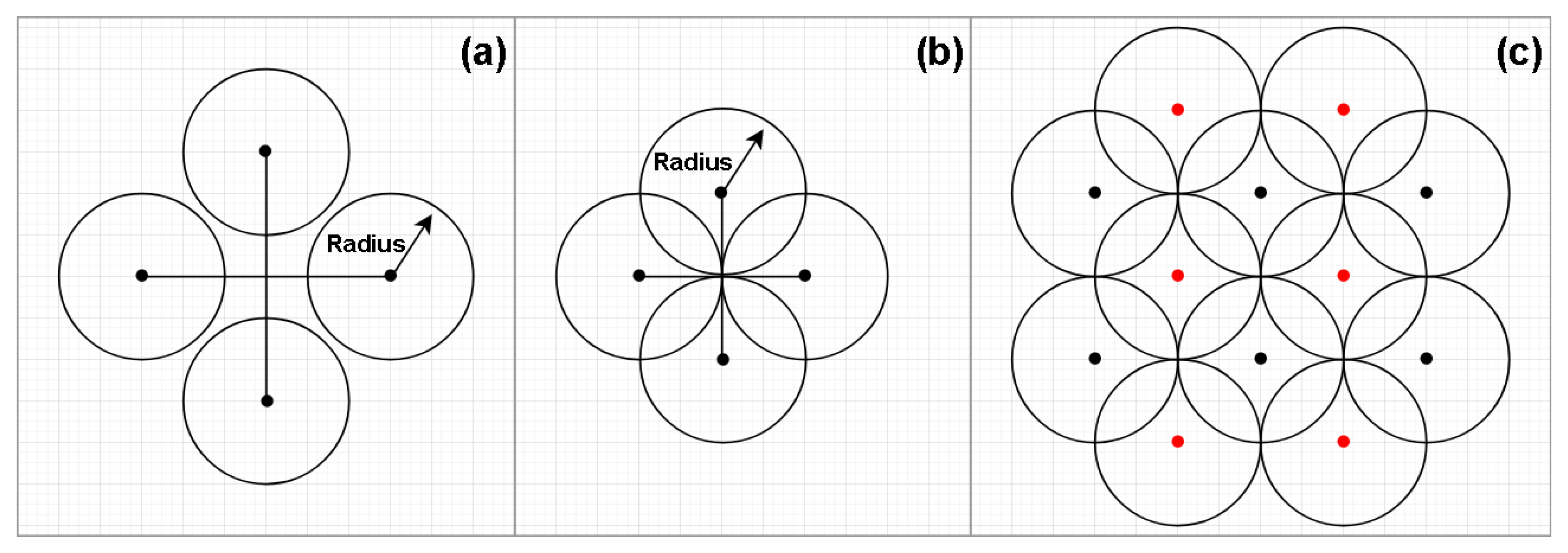
Once the set of coordinates were generated, we discarded the points outside the geographic bounds of the study area. This can be done by using a GIS or a spatial database, for example. However, as shown in Figure 1, given the limitations of this type of search, the coordinates need to respect a predefined spacing, leading to the problem of overlapping radii. In practice, this means that, during the search, the same POI could be returned as result of different requests. We solved this problem by filtering the final dataset using the unique ID provided by Facebook for each POI.
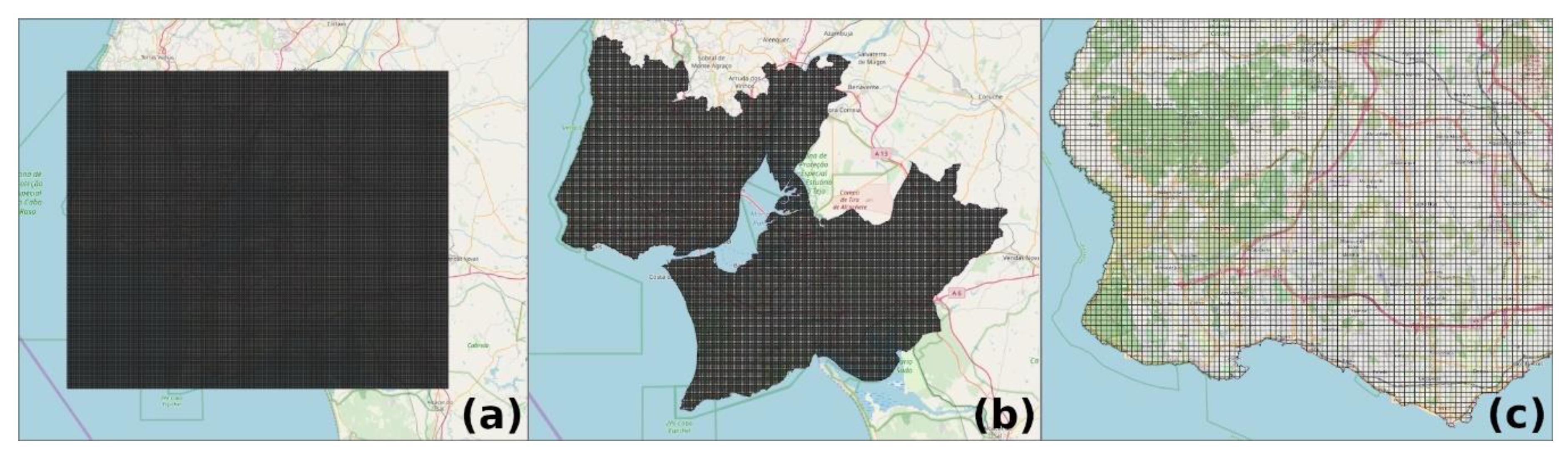
Our software stored the generated coordinates in a database table. Figure 2 shows the steps involved in filtering these points to make them ready for processing. Initially, the set of coordinates generated covers the entire region, according to the four parameters given by the user. This can be seen when creating a layer in GIS software using these points. In this study, we performed a special query directly to the database, based on a polygon saved in a table, which contains the information regarding the geographic bounds of the study area. As a result, only the points within the limits were kept. Although we chose to manipulate the data directly with SQL, the same goal may be easily reached by performing an intersection through a GIS application.
After generating geographic coordinates, the developed application processed them by making searches though a service called “Places Search API for Web” [43,44], provided by Facebook, to collect the data. For each coordinate, the Facebook API returned all POIs in the given radius. When returned, obtained POI data were stored in a database table. As each request take some seconds, the necessary time to collect the data depends on size of the region and, hence, the number of coordinates to be processed. After finishing, it is necessary to filter the final dataset in order to eliminate repeated POIs. Once again, in this case, this was done by manipulating the table directly in the database. For solving this specific problem, we think this is the best approach, given its simplicity and efficacy.
The data used in this work were collected in the scope of another project, and, for this reason they were first obtained for the whole country territory. However, as described before, in the experience we present here, our focus was the LMA. By using the software that we developed, we collected 171,177 POIs distributed along continental Portugal, from which 17,777 were located in the LMA. Considering that each POI can belong to more than one category, the collected dataset presents a total of 24,144 examples in the study area, which were used for extracting features to train the models.
The last step in the POI collection process is to get the Facebook Places taxonomy. We chose to do this through the API, as this was simple and fast. Although each collected POI has an attribute containing a list of all categories to which it belongs, some operations need to be done to link it to the taxonomy obtained separately. We did some manipulation using SQL in order to establish these connections. This step is optional; however, it is highly recommended because the list of categories returned with each POI has no hierarchical structure by itself, and, because of this, the final analysis result may not be so valuable when this taxonomy is unknown.
3.3. Ground Truth Data
CORINE land cover (CLC) [45,46] is basically a dataset representing the use and the coverage of the geographic areas over Europe. It was created as an initiative of the European Environment Agency, in a partnership with the member states. As a thematic cartography, CLC data are mainly produced by image interpretation, often using automatic or semi-automatic solutions available in GIS applications. The dataset can be downloaded in either a raster or vector format, with a minimum mapping unit (MMU) of 25 hectares (ha) for areal phenomena and a minimum width of 100 m for linear phenomena. According to its official nomenclature [47], CLC data are divided in 44 classes over three hierarchical levels. It was first released in 1990 and was updated in 2000, 2006, 2012, and 2018. For our analysis, we utilized the latest version in the format of vector data.
Data Preparation
We adopted a grid-based methodology [48] to represent the land parcels for classification. This method involved creating cells uniformly distributed over the study area. By using a GIS application, a grid in which each cell is 250 meters long/250 meters wide was automatically built, as shown in Figure 3. When created, the grid is a square composed by polygons with a chosen size. In order to keep only the cells inside the study area, we performed an intersection operation. The resulting grid was stored on a database table. For each cell, a spatial attribute that represents its centroid was included. This attribute is essential when generating features for training the predictive model.
After creating the grid, we extracted the LULC class for each cell, based on the CORINE data. It was assumed that there was only one class per land parcel. For example, if in a given cell there is 20% of land covered by class “111. Continuous urban fabric” and in the remaining 80%, the predominant class is “112. Discontinuous urban fabric”, we consider the one that represents most of the space—i.e., the last one. However, before extracting the dominant class for each cell, we organized the dataset class structure, keeping two levels and enabling the possibility to easily classify the units later. Table 2 shows the new class structure. This operation was performed by using a “dissolve” tool available in almost every modern GIS application, which provides the possibility of merging polygons from vector data.
Considering the 15 classes obtained through the reorganization process we applied, after preparing the grid, we obtained 81,238 cells for the study area. Each cell is available for extracting features to be used as training data for the models. The exact number of examples used in each scenario is described in Section 4.
3.4. Feature Extraction
We extracted four distinct types of features based on the collected POI categories and their respective levels, which range from 1 to 6 in the Facebook Places taxonomy [49]. Through an exploratory analysis, we decided to focus on all categories belonging to levels 2, 3, 4, and 5, considering that level 1 is highly generic and level 6 is too specific, presenting only restaurant service categories. Table 3 shows the extracted attribute groups.
As the optimum radius distance, we analyzed 2500, 5000 and 10,000 meters, where the last one proved to be capable of generating the best models. To find the proportion of POIs, this was computed by the following calculation for each category: The amount of points inside the radius, divided by the total of POIs belonging to the category. Considering all feature sets, for all levels, we extracted 5928 attributes in total, with 500 of them belonging to group 1, 1808 to group 2, 2888 to group 3, and the remaining 732 to group 4.
3.5. Feature Selection
After extracting the POI attributes, we first used a correlation matrix to analyze the relevance of each feature type. We noticed that attributes belonging to group 2 presented extremely low correlation with LULC classes. Because of this, we discarded these features. Regarding the features in group 4, we verified that they present almost the same relevance as the attributes belonging to group 3. As the proportion of POI demands more computational power to be calculated, when compared to their amount in a given cell radius, we decided to keep group 3 instead of 4.
As we intended to explore the potential of metrics extracted from POI data for classifying LULC, considering the remain 3388 attributes, for each scenario, we applied a ranking method [50] in order to select the most valuable feature set. Different criteria, including the Information gain, Gain ratio and Gini index, were tested in this process. We chose this approach because it is usually faster and consumes less resources when compared to other methods. By using this technique, we selected different attribute sets which were employed for classification tests. The number of attributes selected in each scenario is presented in Section 4. A list of all feature sets used is available online at http://tiny.cc/9eq8rz.
3.6. Classification
As presented in the state-of-the-art section, among the many different scientific studies we analyzed, the use of various techniques was observed. Some of them are used for data preparation and preprocessing, and others for classification tasks. However, for creating a model capable of classifying land use by using numeric attributes, we believe that it is possible to successfully employ a powerful method which is not usually seen in this context, namely, an artificial neural network (ANN). We tested different scenarios using an ANN, as presented in the next section. The parametrization details are shown in Table 4. As evaluation metrics, the following were adopted: Accuracy, F-score, Kappa, precision and recall. For training the models, we adopted a 10-fold cross-validation technique. RapidMiner Studio [51] was utilized for the classification tests we conducted, and the details for ANN algorithm implementation in this software can be seen in the official documentation [52].
4. Results and Discussion
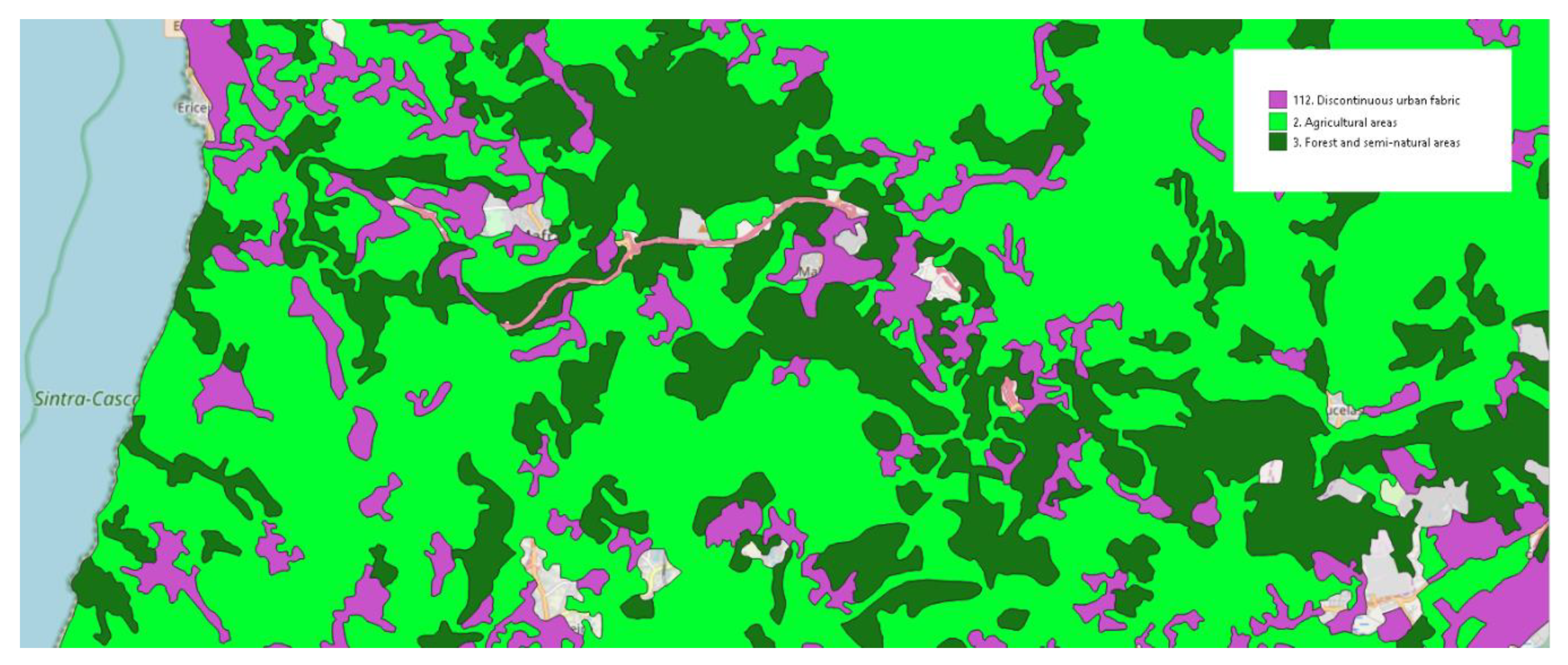
As we noticed in a previously conducted exploratory analysis, a geographic proximity pattern between classes “2. Agricultural areas”, “3. Forest and semi-natural areas”, and “112. Discontinuous urban fabric” seems to exist. Considering this evidence, some preliminary experiments were performed (not presented here), in which we noticed that the models generated when using these three classes together tend to present low performance. For this reason, in most of the experiments approached below, we decided to consider these classes separately.
In the first classification test, we used a dataset containing 144 attributes. Table 5 shows the results of the model evaluation. For this experience, we chose four distinct classes as the final objective for classification: (1) “2. Agricultural areas”; (2) “111. Continuous urban fabric”; (3) “112. Discontinuous urban fabric”; (4) “121. Industrial or commercial units and public facilities”. The training was made by using 2667 examples from the class 121 and 3000 examples for each of those remaining. As seen, the precision and recall of class 112 are both inferior when compared to the others, while the model seems capable of better distinguishing for class 2 among all of them.
As with the previous experiment, we also performed a test based on a model trained using four classes. However, in this test we used the class “3. Forest and semi-natural areas” instead of class “2”. Through the automatic selection method described before, we chose 157 attributes. The results obtained can be seen in Table 6. They show that, in general, the model presents almost no difference when compared to that created in the test before, although we used the same 3000 examples from each class, except for class 121, for which we used 2667 examples.
In the third experiment performed, we also used classes 111 and 121. In order to investigate how far a model can successfully distinguish forests, semi-natural areas, and agricultural land parcels from dense urban spaces and industrial areas, we decided to include classes 2 and 3 for training the model. As with the tests carried out previously, we also adopted a dataset composed by 11,667 examples, although containing 142 attributes—i.e., 15 less than used before. According to the information available in Table 7, the model evaluation shows that, in dense urban areas, the classifier reaches better results, compared to the other classes.
Replacing class 121 with class 112, we trained a new model, recurring to a subsample composed of 4000 examples from each class, except one representing continuous urban fabric parcels, for which only 3043 examples were available. The mentioned dataset has 158 attributes and through the model evaluation we obtained the results listed in Table 8.
In order to complement the presented experiments, in a new scenario considering 221 attributes, we tested a model trained by using three classes that we believed to be highly valuable for land use classification: (1) “2. Agricultural areas”; (2) “111. Continuous urban fabric”; (3) “Industrial or commercial units and public facilities”. The results can be seen in Table 9. For this specific test, we used 4000 examples from class 2, 3043 from class 111, and 2667 from class 121.
Considering that classes 111 and 112 are both from class “1.1. Urban fabric”, we created a model merging the examples from these classes. Using a dataset containing 96 attributes and 4000 examples of the new class, in addition to the other 3043 of class 111 and 2667 of 121, we obtained the results presented in Table 10.
Our last experiment was based on a dataset containing 93 attributes. The model was trained with 4000 examples from classes 111 and 112 together. Another 4000 examples from classes 2 and 3 were mapped to a new class, and 2667, as usual, from class 121. We decided to join examples representing forests and semi-natural regions to those that delimit agricultural areas because of the similarity observed between these two classes via an exploratory analysis we carried out. The results obtained are presented in Table 11.
When analyzing the results obtained, it is possible to discuss some observations. Considering the F-score per class, we can see that, in general, the models tend to show inferior results for the classification of examples that represent discontinuous urban areas. In fact, we can verify this by checking a confusion matrix, where these land parcels are frequently misclassified. As presented in Table 12, the model often tends to predict class 112 as 2 or 111, while it also classifies many examples of agricultural plots as discontinuous urban zones. However, when analyzing the results generated from the model evaluation of scenario 3, it is possible to observe that, when using classes 2, 3, 111 and 121, agricultural lands and forest parcels are those that present the lowest F-score. Examining the confusion matrixes generated for each scenario, we found that these classes are frequently confused with each other.
For trying to find out the main reason forests, agricultural lands, and discontinuous urban areas are classified incorrectly among themselves, we conducted an exploratory analysis. As Figure 4 shows, there is geographical proximity between these classes. Considering that the attributes used represent, in some cases, the distance between each centroid and the nearest POI of each category, and, in others, the amount of points in each category within a radius from each cell center, it is possible to suspect that as many categories are often localized in the dense urban regions, the distance from cells representing these three classes and POIs could be also similar. In other words, this means that the cells representing these three classes are often located far away from many other POI categories. Following this idea, we also think that the amount of POIs from most categories could be lower in these areas, making it difficult to distinguish between them using those features chosen here.
5. Conclusions and Future Work
Initially, in this work, we conducted a survey in order to study a set of works related to the analysis of geographic space. Through a systematic analysis, we have highlighted and discussed the main data types and methods, as well as their utilizations in this context. From the state-of-the-art analysis, we chose to investigate the potential of a specific type of crowdsourced data for land use classification, namely, POIs. We carefully studied the available sources of this information in order to decide which was the most appropriate for our analysis. Based on a service available online, we developed an application to automatically collect POIs for our region of study. Additionally, we applied some data treatment to prepare the data for our experiments.
Based on the POI data, we extracted and analyzed different types of features in order to select those that presented more relevance to be used. Considering the fact that we had a large number of features, we adopted a technique well-established in the literature to automatically rank, among them, the most suitable for each experiment we performed. For land use classification, we chose a grid-based methodology based on a highly reliable ground truth dataset. We defined different scenarios for our tests and adopted a powerful algorithm for classification analysis when using numeric features for all of them.
Although the grid-based method we adopted as part of the methodology we used to prepare the data was previously suggested in the literature, it can be highlighted that, in our study, some differences from the original technique exist. First, our work was based on vector data instead of raster data. We believe that vector data are more efficient for automatic or semi-automatic solutions applied for geographic analysis, because they can aggregate more information related to each parcel of land and can also be easily stored and manipulated directly in a database. Furthermore, the features we adopted are partially different from those used when the method was suggested. Our work provides solid evidence that this methodology works well, and we see these differences that we have implemented as our contribution to the state of the art.
By using an artificial neural network and POI-based data, through different classification scenarios, we achieved values of more than 90% for the accuracy and F-score in the most successful case here. In general, for most experiences, values for these metrics are near to 80%, proving that POIs have the potential to be suggested as a data type for land use classification. Being one of the most common types of crowdsourced data, they are widely and freely available for many countries and can provide relevant contributions by themselves or when combined with other data types, thereby improving results in studies related to the characterization of geographic spaces.
Regarding feature engineering, in this work, we extracted and analyzed four different groups of features. It was verified that only two of them are useful for land use classification. Although we generated a significant number of features, they represent specific metrics extracted from the POI data. Thus, as a suggestion for future work, we recommend analyzing the potential of new metrics—for example, the semantic similarity among POIs—regarding their textual descriptions, which can be added as attributes for training the models, thereby possibly providing better results. Applying deep neural networks for natural language processing (NLP) has been demonstrated as a powerful tool to extract features from texts [13,19]. The adoption of such deep neural networks in our approach could improve the performance of land use classification.
As stated in the state-of-the-art analysis, POI data, as one of the most common crowdsourced data types, are widely available on API services and online repositories. However, as with most of the datasets generated by a large number of users or volunteers, it is very common to find lots of noise in these sets of data. For this reason, we also suggest, as future work, the quality assessment of crowdsourced POI data available from different sources. We have noticed that using reliable datasets is the key for reaching good results in many cases.
In this work, we explored the potential of POI data to characterize geographic spaces—i.e., LULC classification. In the analysis we conducted, we adopted only one source for this kind of dataset. Thus, for future work, we also suggest the investigation of techniques that can be adopted for merging POIs collected from different sources in order to provide additional data enrichment. We believe that using a set of data that is as complete as possible can certainly help to create efficient models.
Supplementary Materials
The datasets and figures used are available online at http://tiny.cc/gq6iqz and the source-code of the application developed to collect the POIs can be found at https://github.com/RibeiroSt/poi-colector-fbp.
Author Contributions
Conceptualization, methodology, data curation, writing—review and editing: Renato Andrade and Ana Alves; investigation, software, writing—original and draft preparation: Renato Andrade; supervision, funding acquisition and project administration: Ana Alves and Carlos Bento. All authors have read and agreed to the published version of the manuscript.
Funding
This research was funded by aicep Portugal Global—Trade & Investment Agency (AICEP).
Conflicts of Interest
The authors declare no conflict of interest. The data used were collected within a preliminary phase of a project that could be implemented by the funders in the future. However, the funders had no role in the design of the study; in the analyses, or interpretation of data; in the writing of the manuscript, nor in the decision to publish the results.
References
- Susanti, R.; Soetomo, S.; Buchori, I.; Brotosunaryo, P.M. Smart Growth, Smart City and Density: In Search of The Appropriate Indicator for Residential Density in Indonesia. Procedia-Soc. Behav. Sci. 2016, 227, 194–201. [Google Scholar] [CrossRef] [Green Version]
- Liu, X.; He, J.; Yao, Y.; Zhang, J.; Liang, H.; Wang, H.; Hong, Y. Classifying urban land use by integrating remote sensing and social media data. Int. J. Geogr. Inf. Sci. 2017, 31, 1675–1696. [Google Scholar] [CrossRef]
- Zhang, Y.; Li, Q.; Huang, H.; Wu, W.; Du, X.; Wang, H. The combined use of remote sensing and social sensing data in fine-grained urban land use mapping: A case study in Beijing, China. Remote Sens. 2017, 9, 865. [Google Scholar] [CrossRef] [Green Version]
- Zhang, X.; Du, S.; Wang, Q. Hierarchical semantic cognition for urban functional zones with VHR satellite images and POI data. ISPRS J. Photogramm. Remote Sens. 2017, 132, 170–184. [Google Scholar] [CrossRef]
- NOAA. National Ocean Service Website. What Is the Difference between Land Cover and Land Use? 2018. Available online: https://oceanservice.noaa.gov/facts/lclu.html (accessed on 13 March 2019).
- Gao, S.; Janowicz, K.; Couclelis, H. Extracting urban functional regions from points of interest and human activities on location-based social networks. Trans. GIS 2017, 21, 446–467. [Google Scholar] [CrossRef]
- Blaschke, T.; Hay, G.J.; Kelly, N.M.; Lang, S.; Hofmann, P.; Addink, E.A.; Feitosa, R.Q.; Van Der Meer, F.; Van Der Werff, H.; Van Coillie, F.; et al. Geographic Object-Based Image Analysis - Towards a new paradigm. ISPRS J. Photogramm. Remote Sens. 2014, 87, 180–191. [Google Scholar] [CrossRef] [Green Version]
- Terroso-Saenz, F.; Muñoz, A. Land use discovery based on Volunteer Geographic Information classification. Expert Syst. Appl. 2020, 140, 112892. [Google Scholar] [CrossRef]
- Xing, H.; Meng, Y. Integrating landscape metrics and socioeconomic features for urban functional region classification. Comput. Environ. Urban Syst. 2018, 72, 134–145. [Google Scholar] [CrossRef]
- Brennan, R.; Webster, T.L. Object-oriented land cover classification of lidar-derived surfaces. Can. J. Remote Sens. 2006, 32, 162–172. [Google Scholar] [CrossRef]
- Gong, B.; Im, J.; Mountrakis, G. An artificial immune network approach to multi-sensor land use/land cover classification. Remote Sens. Environ. 2011, 115, 600–614. [Google Scholar] [CrossRef]
- Qi, Z.; Yeh, A.G.O.; Li, X.; Lin, Z. A novel algorithm for land use and land cover classification using RADARSAT-2 polarimetric SAR data. Remote Sens. Environ. 2012, 118, 21–39. [Google Scholar] [CrossRef]
- Yao, Y.; Li, X.; Liu, X.; Liu, P.; Liang, Z.; Zhang, J.; Mai, K. Sensing spatial distribution of urban land use by integrating points-of-interest and Google Word2Vec model. Int. J. Geogr. Inf. Sci. 2017, 31, 825–848. [Google Scholar] [CrossRef]
- Zhang, X.; Du, S.; Wang, Q. Integrating bottom-up classification and top-down feedback for improving urban land-cover and functional-zone mapping. Remote Sens. Environ. 2018, 212, 231–248. [Google Scholar] [CrossRef]
- Huang, B.; Zhao, B.; Song, Y. Urban land-use mapping using a deep convolutional neural network with high spatial resolution multispectral remote sensing imagery. Remote Sens. Environ. 2018, 214, 73–86. [Google Scholar] [CrossRef]
- Durduran, S.S. Automatic classification of high resolution land cover using a new data weighting procedure: The combination of k-means clustering algorithm and central tendency measures (KMC-CTM). Appl. Soft Comput. J. 2015, 35, 136–150. [Google Scholar] [CrossRef]
- Deng, Z.; Zhu, X.; He, Q.; Tang, L. Land use/land cover classification using time series Landsat 8 images in a heavily urbanized area. Adv. Sp. Res. 2019, 63, 2144–2154. [Google Scholar] [CrossRef]
- Zhong, Y.; Zhu, Q.; Zhang, L. Scene classification based on the multifeature fusion probabilistic topic model for high spatial resolution remote sensing imagery. IEEE Trans. Geosci. Remote Sens. 2015, 53, 6207–6222. [Google Scholar] [CrossRef]
- Zhai, W.; Bai, X.; Shi, Y.; Han, Y.; Peng, Z.-R.; Gu, C. Beyond Word2vec: An approach for urban functional region extraction and identification by combining Place2vec and POIs. Comput. Environ. Urban Syst. 2019, 74, 1–12. [Google Scholar] [CrossRef]
- García-Palomares, J.C.; Salas-Olmedo, M.H.; Moya-Gómez, B.; Condeço-Melhorado, A.; Gutiérrez, J. City dynamics through Twitter: Relationships between land use and spatiotemporal demographics. Cities 2018, 72, 310–319. [Google Scholar] [CrossRef]
- Yuan, J.; Zheng, Y.; Xie, X. Discovering Regions of Different Functions in a City Using Human Mobility and POIs. SIGKDD Int. Conf. Knowl. Discov. Data Min. 2012. [Google Scholar] [CrossRef]
- Liu, X.; Niu, N.; Liu, X.J.; Jin, H.; Ou, J.P.; Jiao, L.M.; Liu, Y.L. Characterizing mixed-use buildings based on multi-source big data. Int. J. Geogr. Inf. Sci. 2018, 32, 738–756. [Google Scholar]
- Jendryke, M.; Balz, T.; McClure, S.C.; Liao, M. Putting people in the picture: Combining big location-based social media data and remote sensing imagery for enhanced contextual urban information in Shanghai. Comput. Environ. Urban Syst. 2017, 62, 99–112. [Google Scholar] [CrossRef] [Green Version]
- Lansley, G.; Longley, P.A. The geography of Twitter topics in London. Comput. Environ. Urban Syst. 2016, 58, 85–96. [Google Scholar] [CrossRef] [Green Version]
- Cheng, Z.; Caverlee, J.; Lee, K.; Sui, D.Z. Exploring Millions of Footprints in Location Sharing Services. Int. Conf. Weblogs Soc. Media 2011, 2010, 81–88. [Google Scholar]
- Arsanjania, J.J.; Vaz, E. An assessment of a collaborative mapping approach for exploring land use patterns for several European metropolises. Int. J. Appl. Earth Obs. Geoinf. 2015, 35, 329–337. [Google Scholar] [CrossRef]
- Yuan, N.J.; Zheng, Y.; Xie, X.; Wang, Y.; Zheng, K.; Xiong, H. Discovering urban functional zones using latent activity trajectories. IEEE Trans. Knowl. Data Eng. 2015, 27, 712–725. [Google Scholar] [CrossRef]
- Gong, L.; Liu, X.; Wu, L.; Liu, Y. Inferring trip purposes and uncovering travel patterns from taxi trajectory data. Cartogr. Geogr. Inf. Sci. 2016, 43, 103–114. [Google Scholar] [CrossRef]
- Trevino, A. Introduction to K-Means Clustering. Oracle + DataScience.com. 2016. Available online: https://www.datascience.com/blog/k-means-clustering (accessed on 20 March 2019).
- Jiang, S.; Alves, A.; Rodrigues, F.; Ferreira, J.; Pereira, F.C. Mining point-of-interest data from social networks for urban land use classification and disaggregation. Comput. Environ. Urban Syst. 2015, 53, 36–46. [Google Scholar] [CrossRef] [Green Version]
- Patel, S. Chapter 2: SVM (Support Vector Machine)—Theory. Machine Learning 101. 2017. Available online: https://medium.com/machine-learning-101/chapter-2-svm-support-vector-machine-theory-f0812effc72 (accessed on 10 June 2019).
- Sotiropoulos, D.N.; Tsihrintzis, G.A. Machine Learning Paradigms. In Machine Learning Paradigms: Artificial Immune Systems and Their Applications in Software Personalization; Springer International Publishing: Cham, Switzerland, 2017; pp. 107–129. [Google Scholar]
- Zhang, X.; Du, S. A Linear Dirichlet Mixture Model for decomposing scenes: Application to analyzing urban functional zonings. Remote Sens. Environ. 2015, 169, 37–49. [Google Scholar] [CrossRef]
- Lilleberg, J.; Zhu, Y.; Zhang, Y. Support vector machines and word2vec for text classification with semantic features. In Proceedings of the 2015 IEEE 14th International Conference on Cognitive Informatics & Cognitive Computing (ICCI*CC), Beijing, China, 6–8 July 2015; pp. 136–140. [Google Scholar]
- Zhang, L.; Zhang, L.; Du, B. Deep learning for remote sensing data: A technical tutorial on the state of the art. IEEE Geosci. Remote Sens. Mag. 2016, 4, 22–40. [Google Scholar] [CrossRef]
- Zhan, X.; Ukkusuri, S.V.; Zhu, F. Inferring Urban Land Use Using Large-Scale Social Media Check-in Data. Netw. Spat. Econ. 2014, 14, 647–667. [Google Scholar] [CrossRef]
- Frias-Martinez, V.; Frias-Martinez, E. Spectral clustering for sensing urban land use using Twitter activity. Eng. Appl. Artif. Intell. 2014, 35, 237–245. [Google Scholar] [CrossRef] [Green Version]
- Yao, Y.; Liang, H.; Li, X.; Zhang, J.; He, J. Sensing urban land-use patterns by integrating Google Tensorflow and scene-classification models. Int. Arch. Photogramm. Remote Sens. Spat. Inf. Sci.-ISPRS Arch. 2017, 42, 981–988. [Google Scholar] [CrossRef] [Green Version]
- Song, J.; Lin, T.; Li, X.; Prishchepov, A.V. Mapping Urban Functional Zones by Integrating Very High Spatial Resolution Remote Sensing Imagery and Points of Interest: A Case Study of Xiamen, China. Remote Sens. 2018, 10, 1737. [Google Scholar] [CrossRef] [Green Version]
- Zhang, C.; Sargent, I.; Pan, X.; Li, H.; Gardiner, A.; Hare, J.; Atkinson, P. An object-based convolutional neural network (OCNN) for urban land use classification. Remote Sens. Environ. 2018, 216, 57–70. [Google Scholar] [CrossRef] [Green Version]
- Flores, E.; Zortea, M.; Scharcanski, J. Dictionaries of deep features for land-use scene classification of very high spatial resolution images. Pattern Recognit. 2019, 89, 32–44. [Google Scholar] [CrossRef]
- Zhang, C.; Sargent, I.; Pan, X.; Li, H.; Gardiner, A.; Hare, J.; Atkinson, P. Joint Deep Learning for land cover and land use classification. Remote Sens. Environ. 2019, 221, 173–187. [Google Scholar] [CrossRef] [Green Version]
- Facebook. Places Search API for Web. Available online: https://developers.facebook.com/docs/places/web/search/ (accessed on 8 July 2020).
- Facebook. Place Information. Available online: https://developers.facebook.com/docs/graph-api/reference/place-information (accessed on 8 July 2020).
- Copernicus. CORINE Land Cover. Available online: https://land.copernicus.eu/pan-european/corine-land-cover (accessed on 2 March 2020).
- Copernicus. CLC 2018. Available online: https://land.copernicus.eu/pan-european/corine-land-cover/clc2018?tab=metadata (accessed on 8 July 2020).
- Kosztra, B.; Büttner, G.; Hazeu, G.; Arnold, S. Updated CLC illustrated nomenclature guidelines. 2019. [Google Scholar]
- Calegari, G.R.; Carlino, E.; Peroni, D.; Celino, I. Extracting urban land use from linked open geospatial data. ISPRS Int. J. Geo-Inf. 2015, 4, 2109–2130. [Google Scholar] [CrossRef]
- Facebook. All Categories. Available online: https://www.facebook.com/pages/category/ (accessed on 16 December 2019).
- Novaković, J.; Strbac, P.; Bulatović, D. Toward optimal feature selection using ranking methods and classification algorithms. Yugosl. J. Oper. Res. 2011, 21, 119–135. [Google Scholar] [CrossRef]
- RapidMiner. RapidMiner | Data Science & Machine Learning Platform. 2020. Available online: https://rapidminer.com/ (accessed on 18 June 2019).
- RapidMiner. Neural Net. Available online: https://docs.rapidminer.com/latest/studio/operators/modeling/predictive/neural_nets/neural_net.html (accessed on 8 July 2020).
Figure 1.
Coordinate generation. As seen in (a), if the distances between the points are too large, the application will not be able to cover the whole area, so, the most reasonable configuration may be that in (b). By adopting this configuration, the final pattern is shown in (c), where we can see that the red points are slightly displaced when compared to the black points. This configuration allows the software to cover more area with less overlapping areas.

Figure 2.
Set of coordinates generated to perform the search. As seen in (a), the points were initially distributed over the entire area inside the square stablished based on limits given by user; (b) shows the points outside geographic limits of the country; (c,d) represent the positions of the final coordinates after filtering.
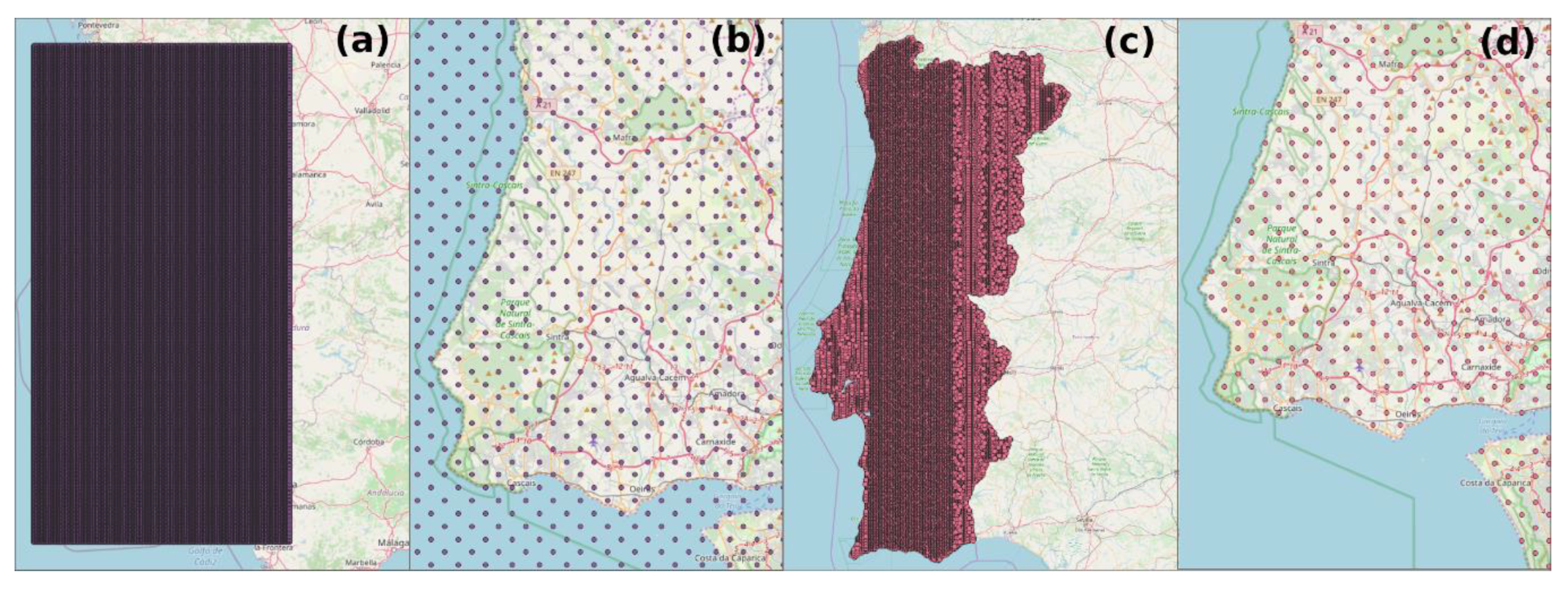
Figure 3.
Grid where each cell represents a land unit to be classified. When created, the grid looks like (a); after the intersection, only the cells inside the geographic bounds of the study area were kept, as we can see in (b,c).
Figure 3.
Grid where each cell represents a land unit to be classified. When created, the grid looks like (a); after the intersection, only the cells inside the geographic bounds of the study area were kept, as we can see in (b,c).

Figure 4.
Geographic proximity between forests, agricultural lands, and discontinuous urban areas.

Table 1.
Data types and methods often adopted for land use analysis.
| Ref. | Data | Method | Objective |
|---|---|---|---|
| [37] | Twitter activity | Self-organizing maps (SOM) | Land segmentation with geolocated data |
| Spectral clustering | Detect urban land uses | ||
| [36] | Location-based social networks (LBSN) user activities, points of interest (POIs) | Laplacian score (LS) | Feature selection |
| Clustering (various algorithms) | Land use inference | ||
| Naïve Bayes (NB); Support vector machine (SVM); random forest (RF) | Classify land use | ||
| [30] | Points of interest (POIs), aggregate census employment data, boundaries of towns | POI matching algorithm | Map POIs from one source to another |
| Bayesian networks; tree-based learners; instance-based learners; rule-based learners | Classify POIs | ||
| Maximum likelihood estimation (MLE) | Estimate disaggregated land use | ||
| [16] | Land cover dataset (remote images + extra attributes) | Multi-resolution segmentation | Image segmentation |
| K-means | Define data belonging to each class | ||
| Central tendency measures | Get the central tendency measure of each class | ||
| K-nearest neighbor (K-NN); extreme learning machine (ELM); Support vector machine (SVM) | Detection of urban land cover | ||
| [27] | POIs, taxi trajectories, public transit records | Dilatation | Remove unnecessary details for map segmentation |
| Subfield-based parallel thinning algorithm | Extract the skeleton of the road segments | ||
| Two-pass algorithm | Generate segmented regions | ||
| Latent Dirichlet allocation (LDA) | Discovery of region topics using mobility patterns based on mobility semantics and location semantics | ||
| Dirichlet multinomial regression (DMR) | |||
| [4] | Remote sensing images, POIs | Hierarchical semantic cognition (HSC) | Classify urban functional zones |
| Multiresolution segmentation | Segment remote sensing images | ||
| Random forest (RF) | Label categories of land use image objects | ||
| ISO- DATA algorithm | Automatically cluster spatial object patterns | ||
| [3] | OpenStreetMaps (OSM) road network, remote sensing images, POIs, LBSN user posts | Cellular automata model | Generate the urban land use parcels |
| RF | Land use classification | ||
| Object-based classification | Classify preprocessed remote sensing images | ||
| Gray-level co-occurrence matrix (GLCM) | Calculate texture attributes | ||
| [2] | OSM road network, remote sensing images, POIs, LBSN user activities | Scale invariant feature transform (SIFT) | Extract features from remote sensing images |
| K-means | Classify features | ||
| Probabilistic latent semantic analysis (pLSA) | Identify latent semantic features | ||
| LDA | |||
| SVM | Classify urban land use types | ||
| [6] | POIs, LBSN user activities | LDA | Generate summaries of thematic place topics |
| K-means | Group semantically similar regions | ||
| Delaunay triangulation spatial constraints | |||
| Ward clustering | Identify topological and hierarchical relations | ||
| [13] | POIs, traffic analysis zones (TAZ) | Greedy algorithm | Construct the TAZ-based documents |
| Word2Vec | Extract POI vectors | ||
| K-means | Group TAZs | ||
| RF | Land use classification | ||
| [38] | Remote sensing images | TF-IDF algorithm | Transform the word frequencies into semantic features |
| RF | Classify urban land use patterns | ||
| Google Inception v5 | Detect land use patterns | ||
| [9] | POIs, text messages, building-level blocks | LDA | Calculate semantic information from crowdsourced data (text messages) |
| RF | Classify functional regions | ||
| [39] | Remote sensing images, POIs, road network | Example-based feature extraction | Produce a binary built-up/non-built-up land cover map |
| Multi-resolution segmentation | Image segmentation | ||
| Object-based classification | Urban land cover classification | ||
| [15] | Remote sensing images, road blocks | Skeleton-based decomposition method | Decompose multispectral image |
| Semi-transfer deep convolutional neural network | Land use mapping | ||
| [22] | LBSN user activities, remote sensing images, taxi trajectories, POIs | Inverse distance weight (IDW) function | Construct the relationships of different data types |
| Kernel density estimation | Infer buildings’ mixed-use functions | ||
| A modified Bayesian model | Calculate the probability of purposes of passengers based on taxi data and POIs | ||
| [14] | Remote sensing images, road blocks | Multiresolution segmentation | Segment blocks |
| Hierarchical Semantic Cognition (HSC) | Bottom-up classification (land covers and functional zones) | ||
| Inverse hierarchical semantic cognition (IHSC) | Optimize classification results | ||
| [40] | Remote sensing images | Object-based convolutional neural network | Urban land use classification |
| [19] | POIs, origin–destination (OD) datasets | K-means | Group POIs and cluster neighborhood areas |
| POI frequency analysis | Annotate the function of each region | ||
| RF | Evaluate and compare the model accuracy | ||
| Place2vec | Extract and classify urban functional regions | ||
| [41] | Remote sensing images | ResNet-50 DCNN | Extract the deep features from images |
| [17] | Remote sensing images | Space–time fusion algorithm (ESTARFM) | Fuse original data pairs at two periods |
| Multiresolution segmentation | Segment the images | ||
| SVM | Extract land use and land cover types | ||
| [42] | Remote sensing images | Joint deep learning (JDL) | Land use and land cover classification |
| [8] | Flickr photos, POIs | Hierarchical clustering LDA RF Multi-label classification | Cluster photos to identify most dynamic regions Extract topics from photo descriptions Land use classification on POI taxonomy (ground truth) using LDA topics as features |
| Ours | POIs | Artificial neural network (ANN) (please see Section 3.6) | Using CORINE (CLC) dataset as ground truth (Section 3.3), extract features from POI taxonomy (Section 3.4) to learn a land use classifier |
Table 2.
CORINE class structures after applying a dissolve operation.
| Class | Subclass |
|---|---|
| Class 1.1. Urban fabric | 111. Continuous urban fabric |
| 112. Discontinuous urban fabric | |
| Class 1.2. Industrial, commercial and transport units | 121. Industrial or commercial units and public facilities |
| 122. Road and rail networks and associated land | |
| 123. Port areas | |
| 124. Airports | |
| Class 1.3. Mine, dump and construction sites | 131. Mineral extraction sites |
| 132. Dump sites | |
| 133. Construction sites | |
| Class 1.4. Artificial non-agricultural vegetated areas | 141. Green urban areas |
| 142. Sport and leisure facilities | |
| 2. Agricultural areas | 2. Agricultural areas |
| 3. Forest and semi-natural areas | 3. Forest and semi-natural areas |
| 4. Wetlands | 4. Wetlands |
| 5. Water bodies | 5. Water bodies |
Table 3.
Feature set extracted from POIs and their categories.
| Feature Set | Description |
|---|---|
| Group 1 | Distance from each cell centroid to the closest POI of each category |
| Group 2 | Distance from each cell centroid to the most distant POI of each category |
| Group 3 | Amount of POIs belonging to each category inside a radius from each centroid |
| Group 4 | Proportion of POIs belonging to each category inside a radius from each centroid |
Table 4.
Parameters used in the classifier.
| Classifier | Parameter | Value |
|---|---|---|
| Artificial neural network—ANN | Hidden layers | (Number of attributes + number of classes)/2 + 1 |
| Training cycles | 200 | |
| Learning rate | 0.01 | |
| Momentum | 0.9 | |
| Shuffle | True | |
| Normalize | True | |
| Error epsilon | 0.0001 |
Table 5.
Results from scenario 1.
| Measure | Value | Class | Prec. | Recall | F-Score |
|---|---|---|---|---|---|
| Accuracy | 77.41 | 2. Agricultural areas | 83.32 | 76.30 | 79.66 |
| Weighted F-score | 77.39 | 111. Continuous urban fabric | 78.74 | 88.24 | 83.22 |
| Kappa | 0.70 | 112. Discontinuous urban fabric | 69.94 | 71.65 | 70.78 |
| Weighted recall | 77.89 | 121. Industrial or commercial units and public facilities | 79.17 | 75.37 | 77.22 |
| Weighted precision | 78.22 |
Table 6.
Results from scenario 2.
| Measure | Value | Class | Prec. | Recall | F-Score |
|---|---|---|---|---|---|
| Accuracy | 78.53 | 3. Forest and semi-natural areas | 87.27 | 82.45 | 84.79 |
| Weighted F-score | 72.14 | 111. Continuous urban fabric | 76.25 | 87.91 | 81.68 |
| Kappa | 0.71 | 112. Discontinuous urban fabric | 74.31 | 70.28 | 72.24 |
| Weighted recall | 78.74 | 121. Industrial or commercial units and public facilities | 75.09 | 74.35 | 74.72 |
| Weighted precision | 78.65 |
Table 7.
Results from scenario 3.
| Measure | Value | Class | Prec. | Recall | F-Score |
|---|---|---|---|---|---|
| Accuracy | 78.01 | 2. Agricultural areas | 76.93 | 66.12 | 71.12 |
| Weighted F-score | 77.86 | 3. Forest and semi-natural areas | 72.90 | 79.07 | 75.86 |
| Kappa | 0.70 | 111. Continuous urban fabric | 87.54 | 90.04 | 88.77 |
| Weighted recall | 78.94 | 121. Industrial or commercial units and public facilities | 76.60 | 80.50 | 78.50 |
| Weighted precision | 78.57 |
Table 8.
Results from scenario 4.
| Measure | Value | Class | Prec. | Recall | F-Score |
|---|---|---|---|---|---|
| Accuracy | 73.34 | 3. Forest and semi-natural areas | 72.84 | 75.58 | 74.18 |
| Weighted F-score | 71.74 | 2. Agricultural areas | 70.04 | 64.65 | 67.24 |
| Kappa | 0.64 | 111. Continuous urban fabric | 82.29 | 89.16 | 85.59 |
| Weighted recall | 74.28 | 112. Discontinuous urban fabric | 69.42 | 67.75 | 68.57 |
| Weighted precision | 73.92 |
Table 9.
Results from scenario 5.
| Measure | Value | Class | Prec. | Recall | F-Score |
|---|---|---|---|---|---|
| Accuracy | 90.21 | 2. Agricultural areas | 93.68 | 91.55 | 92.60 |
| Weighted F-score | 90.20 | 111. Continuous urban fabric | 87.75 | 93.53 | 91.60 |
| Kappa | 0.85 | 121. Industrial or commercial units and public facilities | 85.59 | 84.40 | 84.99 |
| Weighted recall | 89.83 | ||||
| Weighted precision | 89.84 |
Table 10.
Results from scenario 6.
| Measure | Value | Class | Prec. | Recall | F-Score |
|---|---|---|---|---|---|
| Accuracy | 82.31 | 111. Continuous urban fabric & 112. Discontinuous urban fabric | 81.22 | 81.17 | 81.19 |
| Weighted F-score | 82.34 | ||||
| Kappa | 0.73 | 2. Agricultural areas | 86.65 | 83.08 | 84.83 |
| Weighted recall | 82.37 | 121. Industrial or commercial units and public facilities | 77.98 | 82.86 | 80.35 |
| Weighted precision | 82.16 |
Table 11.
Results from scenario 7.
| Measure | Value | Class | Prec. | Recall | F-Score |
|---|---|---|---|---|---|
| Accuracy | 81.88 | 2. Agricultural areas & 3. Forest and semi-natural areas | 84.08 | 84.9 | 84.49 |
| Weighted F-score | 81.89 | ||||
| Kappa | 0.72 | 111. Continuous urban fabric & 112. Discontinuous urban fabric | 79.97 | 81.15 | 80.56 |
| Weighted recall | 81.83 | ||||
| Weighted precision | 81.75 | 121. Industrial or commercial units and public facilities | 81.44 | 78.58 | 79.98 |
Table 12.
Confusion matrix generated in the first scenario.
| 2. Agricultural Areas | 111. Continuous Urban Fabric | 112. Discontinuous Urban Fabric | 121. Industrial or Commercial Units and Public Facilities | |||||
|---|---|---|---|---|---|---|---|---|
| 2. Agricultural areas | 3052 | 76.74% | 15 | 0.49% | 466 | 11.65% | 130 | 4.87% |
| 111. Continuous urban fabric | 83 | 2.09% | 2685 | 88.24% | 409 | 10.23% | 233 | 8.74% |
| 112. Discontinuous urban fabric | 661 | 16.62% | 257 | 8.45% | 2866 | 71.65% | 294 | 11.02% |
| 121. Industrial or commercial units and public facilities | 181 | 4.55% | 86 | 2.83% | 259 | 6.48% | 2010 | 75.37% |
© 2020 by the authors. Licensee MDPI, Basel, Switzerland. This article is an open access article distributed under the terms and conditions of the Creative Commons Attribution (CC BY) license (http://creativecommons.org/licenses/by/4.0/).
Share and Cite
MDPI and ACS Style
Andrade, R.; Alves, A.; Bento, C. POI Mining for Land Use Classification: A Case Study. ISPRS Int. J. Geo-Inf. 2020, 9, 493. https://0-doi-org.brum.beds.ac.uk/10.3390/ijgi9090493
AMA Style
Andrade R, Alves A, Bento C. POI Mining for Land Use Classification: A Case Study. ISPRS International Journal of Geo-Information. 2020; 9(9):493. https://0-doi-org.brum.beds.ac.uk/10.3390/ijgi9090493
Chicago/Turabian StyleAndrade, Renato, Ana Alves, and Carlos Bento. 2020. "POI Mining for Land Use Classification: A Case Study" ISPRS International Journal of Geo-Information 9, no. 9: 493. https://0-doi-org.brum.beds.ac.uk/10.3390/ijgi9090493
Note that from the first issue of 2016, this journal uses article numbers instead of page numbers. See further details here.