Leveraging OSM and GEOBIA to Create and Update Forest Type Maps


Remote Sensing & Geoinformatics Department, Trier University, 54286 Trier, Germany
*
Author to whom correspondence should be addressed.
ISPRS Int. J. Geo-Inf. 2020, 9(9), 499; https://0-doi-org.brum.beds.ac.uk/10.3390/ijgi9090499
Submission received: 29 May 2020
/
Revised: 27 July 2020
/
Accepted: 19 August 2020
/
Published: 21 August 2020
(This article belongs to the Special Issue OpenStreetMap as A Multi-Disciplinary Nexus: Perspectives, Practices and Procedures)
Abstract
:Up-to-date information about the type and spatial distribution of forests is an essential element in both sustainable forest management and environmental monitoring and modelling. The OpenStreetMap (OSM) database contains vast amounts of spatial information on natural features, including forests (landuse=forest). The OSM data model includes describing tags for its contents, i.e., leaf type for forest areas (i.e., leaf_type=broadleaved). Although the leaf type tag is common, the vast majority of forest areas are tagged with the leaf type mixed, amounting to a total area of 87% of landuse=forests from the OSM database. These areas comprise an important information source to derive and update forest type maps. In order to leverage this information content, a methodology for stratification of leaf types inside these areas has been developed using image segmentation on aerial imagery and subsequent classification of leaf types. The presented methodology achieves an overall classification accuracy of 85% for the leaf types needleleaved and broadleaved in the selected forest areas. The resulting stratification demonstrates that through approaches, such as that presented, the derivation of forest type maps from OSM would be feasible with an extended and improved methodology. It also suggests an improved methodology might be able to provide updates of leaf type to the OSM database with contributor participation.
1. Introduction
A key factor for sustainable forest management and forest monitoring is the availability of up-to-date and high spatial resolution information on the state of forest ecosystems. Earth observation data, as well as techniques and methodologies of geoinformatics, can provide valuable contributions to these information needs, while also being suitable in respect to the trade-off between spatial details, update cycles and production costs. As new earth observation data is being released and made publicly accessible, the integration of different data sources and data fusion leads to an increased quality of forest type products [1,2,3,4,5,6]. Considering the required spatial detail and the usability of these products in local forest studies, accurate mapping of the spatial distribution of forest types remains a challenge [3,6]. Open spatial datasets covering forest and forest-related information are available on continental scale for Europe through the Copernicus Land Monitoring Service (https://land.copernicus.eu/), e.g., CORINE Land Cover (CLC) datasets (with broadleaved, needleleaved and mixed forest classes) and High Resolution Layers (HRL) on tree cover density, dominant leaf type and forest type. Datasets covering only selected areas are e.g., Urban Atlas (UA) for selected urban areas. According to these examples, European-wide datasets are either in a resolution that is induced by the underlying satellite data (i.e., Sentinel-2 and Landsat for HRL leads to a spatial resolution of 20 m) or provided with a minimum mapping unit (MMU) not sufficient in a local context (i.e., CLC with 25 ha MMU). UA is produced for specific regions with 2 to 2.5 m spatial resolution and a MMU of 1 ha, but only includes a general forest class without further information on leaf type. Local datasets can be of high spatial and thematic detail, but are rarely accessible by the public.
Very high resolution (VHR) imagery based on aerial or satellite acquisitions are a huge asset for forest inventories. Due to the acquisition in regular intervals for whole states and countries, aerial imagery remains an important data source [7,8,9], while VHR satellite imagery captivates with additional spectral information [10,11]. Due to the high spatial resolution in the sub-meter scale and the option to derive textural parameters, aerial imagery and VHR satellite imagery constitute important image source [9,12,13,14]. Additionally, advances in processing VHR imagery further increase the potential. One of such advances is the field of geographic object-based image analysis (GEOBIA) [15]. In GEOBIA, image segmentation and classification procedures are used to delineate homogenous image segments for analysis. GEOBIA has its strength especially on VHR imagery, as objects tend to be larger than the pixel. Using GEOBIA, processing is based on segments instead of individual pixels [15,16,17,18]. Methods of GEOBIA have proven to be superior to traditional pixel-based classification in spatially high resolution imagery as they lead to a large reduction of the salt-and-pepper effect of many pixel-based classification methods [15,19,20]. The integration of existing vector information (e.g., existing land parcels) has been identified as an advantageous information source that can be used as constraints in the segmentation process in GEOBIA to control the segmentation process with a focus on detecting differences inside already known units [15,21,22,23,24].
Since access to official forest databases is often limited or only available for state owned forests, open datasets become more and more important. As such, volunteered geographic information (VGI) can play a vital role in further advancing GEOBIA concepts. VGI is gaining more and more attention in research and publications, as well as for administrative and commercial applications, and interest has risen over the past decade [25,26,27]. The integration of VGI and remote sensing offers new options in image processing that need to be explored [28]. In respect to vector boundaries fit to be used in the segmentation stage of GEOBIA, OpenStreetMap (OSM) constitutes an extensive data source. Since its creation in 2004, the OSM database and its active contributors have grown steadily to create a detailed map of the world as open data [29,30,31]. OSM geometry in combination with the associated, describing tags contributes to global information needs for many different sectors (e.g., road networks, building footprints or land use/land cover (LULC) information [23,32,33,34,35,36,37,38,39]). With spatially high resolution, cross-border data-consistency and its free availability, OSM has been able to surpass the data quality of administrative datasets in areas with continuous and active contribution [40,41]. Especially for cross-border studies, the constraints of administrative LULC datasets can constitute problems concerning the cross-border availability, consistency and currency of the investigated features [3].
Especially in studies focusing on land cover and natural features, OSM data have been of recent interest. Schultz et al. (2017) [41] and Yang et al. (2017) [42] produced regional land use maps using training data from OSM in supervised classifications of earth observation data. Yang (2019) [43] uses a similar approach to derive a land cover classification using OSM as training data and subsequently assesses forest fragmentation through the incorporation of OSM road networks. Upton et al. (2015) [44] combine OSM data with administrative forest data to estimate access to forest recreational services. Limitations in using OSM in these studies have mainly been due to data gaps for natural and land use features that needed to be filled in by additional data sources or by low contribution activity towards LULC features.
Luxembourg pursues an open (spatial) data policy and was therefore chosen as the study area due to the availability of several critical datasets (e.g., infrared aerial imagery and surface objects from the official carto-/topographic database), which can be used as input data for stratification as well as reference data for validation. A preliminary visual data review of OSM in Luxembourg showed that the mapping of the land use class forest is complete and of spatially high accuracy. Nevertheless, a further stratification into thematic valid subdivisions is often missing, as only half of the forest areas in Luxembourg have been tagged with additional information on leaf type (i.e., broadleaved or needleleaved). The prominence of forest areas with the leaf type mixed is seen as problematic. Given there is a lack of guidance on minimum mapping units in OSM, tagging a large forest area as mixed is technically correct, if the forest area is composed of patches of broadleaved and needleleaved forest. Unfortunately, this way of tagging is ambiguous as it is not able to describe the stratification of the leaf types broadleaved and needleleaved inside the forest polygons. True mixed forest areas would generally be hard to delineate into stratified subdivisions as the mix of needleleaved and broadleaved forest type makes it hard to identify boundaries between the forest types. Data exploration showed that the polygons tagged as mixed forests in OSM include many areas that are comprised of visually recognizable stands of different forest types. A delineation of forest types would thus increase the spatial and thematic detail in the OSM database. A detailed delineation of forest types with information on their leaf types could also increase the potential of using and integrating OSM data in land cover classifications, planning and modelling.
In order to increase the applicability of OSM data for forest research and applications, subdivisions of forest relations need to be mapped and those subdivisions need to be enriched with thematic content (i.e., broadleaved and needleleaved). Accurate mapping of the spatial distribution of forest types in a spatial detail that is fit to be used in regional or local studies could be achieved by the integration of OSM data and remote sensing data and methods.
Based on the information needs and the map product requirements, the following research question has been defined: Is it possible to use OSM data and aerial imagery to create, upgrade, update and spatialize forest type maps?
In order to start answering this overarching question, the present study takes a first step in investigating already present OSM forest polygons that could further be stratified into broadleaved or needleleaved forest stands. Several technical challenges in the processing chain have to be solved to achieve this:
- Separation of forest types based on region growing segmentation and aerial imagery inside existing vector boundaries.
- Classification of derived segments.
- Upgrade of OpenStreetMap geometries through spatial and thematic subdivisions of forest type.
OSM data is used regularly in studies, e.g., to update existing datasets [45,46] or to create new datasets based on OSM data [41,42,43], but rarely do these projects generate feedback to the OSM database. Ideally, the investigation would result in an assessment of the feasibility to use GEOBIA to identify subdivisions of existing OSM forest polygons that can subsequently be integrated back into the OSM database with updated keys on leaf_type. On a more basic level, the feasibility study will result in an estimation of the spatial and thematic content in OSM mixed forest polygons for the investigated area and be able to show the opportunities waiting to be further explored using OSM natural/land use data.
2. Study Area
Forests cover 940 km2 of Luxembourg (see Figure 1), which is 36% of the country’s land area with roughly two thirds of the forest area being covered by broadleaved forests [3]. The most representative tree species are: European beech (Fagus sylvatica L.), sessile oak and pedunculate oak (Quercus petraea (Matt.) Liebl.; Quercus robur L.), Norway spruce (Picea abies (L.) H. Karst.), European hornbeam (Carpinus betulus L.) and Douglas fir (Pseudotsuga menziesii (Mirbel) Franco) [47,48].
Luxembourg’s public data portal (https://data.public.lu/en) offers a large variability of geographic datasets useful for the investigation of forest ecosystems, i.e., aerial imagery (RGB and infrared in 20 cm × 20 cm spatial resolution), digital elevation models and datasets on different aspects (i.e., forest areas) from the official carto-/topographic database [49]. The acquisition of the 2018 aerial imagery took place with flights on the 2nd of July, 8th of July, 27th of July and 5th of August [50]. Additional information from the Administration of cadaster and topography include a flight altitude of 3000 m and a native ground sampling distance of 0.20 m. The data is supplied in JPEG2000 format with 8 bit radiometric resolution [50,51].
Data analysis of OpenStreetMap relations and ways showed that forest areas in Luxembourg tagged with key=value pair landuse=forest cover an area of 812 km2, showing that substantial amounts of forest areas in Luxembourg are also represented in the OSM database. Disparities between the two databases are due to forests in the OSM database carrying different tags, like natural=wood or leisure=park. Additionally, there are areas in the official carto-/topographic database that are administratively forests, but do not comprise forest cover at present. Some of these areas are not tagged as forests in the OSM database as the data is constructed by visual inspection of satellite imagery.
OpenStreetMap entities can be described with several tags and further investigation of the tags showed that forests are often additionally tagged with a leaf_type tag. The majority of forest areas is tagged with the leaf_type value mixed (50% of around 3600 forest polygons). Those OSM mixed forest polygons amount to an area of 703 km2, therefore comprising 87% of the whole OSM forest area. OSM broadleaved forest polygons cover 87 km2 and OSM needleleaved forest polygons cover 22 km2. Although leaf_type with the value mixed is technically correct in most of the cases, it misses the potential of OSM to delineate forest types with more detailed tagging of leaf_type=broadleaved or needleleaved in high spatial detail. This information would deliver spatially explicit information that would enrich the database. Subsequently, this information could be used as training data for classifications or as validation data for other forest type maps.
Intersection of the OSM forest polygons with forest polygons from the official carto-/topographic database of Luxembourg resulted in a 785 km2 agreement for forest location. An intersection based on the leaf-type information present in both databases shows a high discrepancy between the two databases. It again shows the high prevalence of OSM forest polygons with leaf type mixed as they encompass 84% of broadleaved and 86% of needleleaved from the official carto-/topographic database. A substantial amount of forest type information is not mapped in the OSM forest polygons with the leaf type mixed, which shows a stratification of leaf types inside the detailed OSM-geometry could provide a valuable contribution to the upgrade and update of forest type maps.
3. Materials and Methods
The entire processing chain (Figure 2) was developed exclusively in open-source software and using open-access data sources. This was deemed very important as the whole data processing can be reproduced by using the mentioned tools, which might encourage similar studies. It is also the prerequisite to be able to unrestrictedly access and to make the results publicly available. Open source software provides access to the latest algorithms and to the underlying source code, which makes it possible to adapt processes as required for specific tasks.
3.1. Selection of OSM Relations
OpenStreetMap vector data with landuse=forest and leaf_type=mixed tags have been acquired using the Overpass Turbo API (http://overpass-turbo.eu/) [52]. Areas crossing the administrative boundary of Luxembourg have subsequently been discarded, as other data sources are only available inside the country’s boundaries. Inconsistencies between the OSM database and the official carto-/topographic database could be investigated in the leaf type mixed classes, which are highly overestimated by the OSM database. This discrepancy is due to the digitization of large polygons in the OSM database, which have a mean size of 37 ha. OSM mixed forest polygons also occupy 87% of the whole forest area, showing that these areas are of large size in tendency. A total of 21 of the larger OSM forest polygons (127 ha to 1365 ha) with the leaf-type value mixed have been selected all over Luxembourg in order to investigate the readiness of the approach in consideration of different ecological stand conditions as well as forest management schemes (Figure 3). These large mixed forest polygons are subsequently used as boundaries in the image segmentation (compare Figure 2).
3.2. Image Segmentation inside OSM Forest Polygons
Region growing approaches have proven to perform well in the segmentation of natural features, like forests, where hard edges might not be present [53,54,55]. The segmentation of the aerial imagery has therefore been carried out with a region growing algorithm implemented in the GRASS GIS i.segment.gsoc module [56]. Region growing algorithms are based on a similarity measure that is calculated for neighboring segments and the most similar neighbors are subsequently merged. The segmentation initializes with each pixel being set as a segment. The merging of individual segments is controlled by a threshold parameter, describing the allowed level of dissimilarity between segments. Therefore, the threshold inherently determines the size of resulting segments as it indicates the maximum difference under which two different segments will still be merged. The calculation of the similarity measure as used in the i.segment.gsoc module is shown in Equation (1). The parameters to be adjusted in the segmentation module are the threshold, radioweight and smoothweight [57].
Radioweight establishes the weight of color and shape towards the calculated difference between segments. If the calculated value v between two segments is below the given threshold, segments will be merged. As soon as no further merges can be made, the parameter minsize forces small segments to be merged with their most similar neighbor, even if the value v is larger than the specified threshold. The parameter smoothweight can be adapted in order to put more weight on either smoothness or compactness of the segments in the hshape contribution of the similarity measure (Equation (1)).
GEOBIA workflows most commonly rely on testing of different parameters and a visual estimation if the segmentation is suitable to solve the presented delineation problem. Automated procedures have been developed in order to find the best parameters for segmentation. The unsupervised parameter optimization (USPO) implemented in the GRASS GIS module i.segment.uspo [58] is such an automated procedure. This unsupervised optimization is based on the research of Espindola et al. (2006) [59] using within-segment homogeneity (an area weighted variance, WV) and between-segment heterogeneity (Moran’s I measure for spatial autocorrelation, MI) to evaluate the overall goodness of segmentations based on different parameter combinations. WV and MI values for each segmentation are scaled according to the maximum and minimum WV and MI values of all segmentations. The segmentation with the highest sum of the scaled values is chosen as the best segmentation. Johnson et al. (2015) [60] further enhanced this optimization by introducing the F-measure, which can be used to give either within-segment homogeneity or between-segment heterogeneity more weight through a parameter α. The parameter α has been set to the value 2 to find optimal segmentations where within-segment homogeneity is given more weight than between-segment heterogeneity [60]. This is based on the assumption that oversegmentation is generally preferred to undersegmentation. In most segmentation procedures, oversegmentation allows more options for post-processing of the segments (e.g., classification, merging) [58,61]. The USPO code has been transferred from the function i.segment.uspo to be used in combination with the i.segment.gsoc module.
The USPO has been developed to select the best segmentation parameter combinations based on different regional subsets in a larger image and choosing the lowest optimal segmentation parameter for segmentation of the whole scene [58]. In the presented study, the regions themselves are bound by the OSM geometry of mixed forest polygons and therefore are used as subsets to determine the best threshold parameter per forest polygon. The OSM forest polygons are imported and segmentations are run subsequently using each OSM forest polygon as mask for the segmentation algorithm. The analysis of the best parameter set was focused on the threshold parameter, while holding radioweight and smoothweight constant at the defaults of 0.9 and 0.5, respectively. Considering comparability between the segmented OSM forest polygons, this local optimization is not ideal. On the other hand, a global threshold is not fit to optimize the segmentation on all OSM forest polygons due to the different spatial contexts (e.g., surrounding topography, forest management schemes or different ecological stand conditions).
Very high resolution R/G/B and IR aerial imagery has been used as segmentation input in order to be able to compare the resulting segmentations based on the omission or inclusion of an infrared band. The aerial images have been resampled to a lower resolution (original 0.2 m × 0.2 m to 2 m × 2 m) due to processing costs, appropriateness for intended target objects and according to the desired minimum segment size. As the target objects are not individual trees, but should constitute forest areas with homogenous leaf-type, 2 m × 2 m resolution leads to segments that are of high spatial detail in delineating the target objects. The original resolution of 0.2 m × 0.2 m would lead to smaller variations in the forest areas to be aggravated. These small variations would lead to unpredictable behavior in the last step of the region growing procedure as the minsize parameter leads to aggregation of 12,500 pixels in order to arrive at the minimum size of 0.05 ha. This is also the most processing cost-intensive part of the region growing procedure as several iterations might be necessary to arrive at the minimum size. The minimum mapping unit has been set to 0.05 ha, which is the lower boundary of the UNFCCC forest definition [62].
3.3. Selection of Training Areas for Classification
As the whole processing chain is based on open data and open software, the training data has been derived directly from the OSM database. It was deemed an important part of the processing chain to focus on an approach that could be operationally employed using the information from the OSM database, without the need to find training data from different sources or to manually construct them out of the aerial imagery. Checking different approaches to derive training data from OSM may give some indication as to whether it is feasible to use already digitized forest polygons from the OSM database or if incorrect keys or rough digitization can become a problem. Concerning the temporal discrepancy between the OSM database and the acquisition of the aerial images, an inspection of the history of OSM forest polygons showed that there is active contribution concerning land use features in the study area and that existing land use features are continuously updated.
Training data was derived by selecting those OSM forest polygons, which include the leaf_type needleleaved or leaf_type broadleaved values. This also assures that the training and target datasets are spatially independent from each other, as polygons are distributed over the whole area of Luxembourg and the training polygons are spatially separate from the OSM mixed forests in which the segments are subsequently classified. Two different training approaches were tested to find out, if a manual selection of appropriate training areas would lead to substantially better classification accuracies than an automated selection. The amount of training areas for each forest type derived by those approaches is recorded in Table 1.
An automatic approach was used to derive all the OSM forest polygons tagged as broadleaved or needleleaved between 0.1 ha and 10 ha, without further checking if those tags are appropriately set. The second approach included manual inspection of OSM Forest polygons by consulting the spatially high resolution aerial imagery. Only those polygons that were tagged appropriately have been kept for training. Table 1 shows that the manual checking significantly reduced the amount of training areas.
3.4. Classification
Classifications in GEOBIA workflows are based on resulting segments instead of pixels. Those segments need to be enriched with additional data, as the result from the segmentation carries no information in addition to the geometric properties. Preparation for the classification was carried out in GRASS GIS by calculating zonal statistics on additional thematic information for each of the segments. The list of calculated variables consists of the radiometric values from the aerial imagery (R/G/B/nIR mean and standard deviation) as well as selected texture measures, which can be derived directly from the aerial images.
Using texture in a GEOBIA classification has shown to be an important additional feature to discriminate forest types and leads to increased classification accuracies [16,63,64]. The perception of an object and discrimination of objects is largely driven by texture and spatial information [15,65]. A successful employment of texture parameters in the classification demands for parameters (window size and sampling distance) to be optimized according to the features that are intended to be detected (e.g., forest stands instead of individual trees). Following the authors in Feng et al. (2015) [66], the green band has been used to calculate the texture measures with a window size of 7 and a sampling distance of 1. Texture measures have been calculated with the GRASS GIS module r.texture [67] which implements developed algorithms on grey level co-occurrence matrices of Haralick et al. [65,68] using 1 m × 1 m aerial imagery. Texture measures have been selected following recommendations of a practical guideline for GLCM feature selection [69] and thus Inverse Difference Moment (IDM), Angular Second Momentum (ASM), Correlation (COR), Entropy (ENT) have been selected as the texture measures to be used in the classification.
Mean and standard deviation for each band of the aerial image and the mean for the selected texture measures have been calculated for all polygons of the training setups (automatic and manual) and for all segments resulting from the segmentation setups (RGB, RGBnIR).
Classification was carried out using the Random Forest classifier [70] with R package Caret in R 3.6.2. [71]. For a complete overview and review of the Random Forest classifier and its use in remote sensing, refer to Belgui and Drăguţ (2016) [72]. The Random Forest classifier has been used successfully in GEOBIA studies and has shown lower sensitivity concerning the selection of features to be used in the classification [73]. Another advantage of the Random Forest classifier (e.g., over Support Vector Machines) is that fewer parameters have to be set and better results can be achieved on multi-source data [72]. Random Forests can also be used to estimate variable importance. Estimation of variable importance is implemented in the R package Caret for different classifiers. In the case of Random Forest, out-of-bag (OOB) samples are used to estimate variable importance and to estimate internal model errors. All models were trained using 10-fold cross-validation with 5 times repetition and using a grid search to tune the parameter mtry, which determines the number of randomly sampled variables to be used at each split of the model. Additionally, due to unbalanced leaf-type classes, especially in the automatic training area selection, a resampling procedure has been used to down sample the majority class (broadleaved).
3.5. Validation
Forest type polygons from the official carto-/topographic database of Luxembourg have been used as the basis for validation. The official forest type polygons also comprise a forest type mixed. This forest type has been removed completely from the validation strategy. Mainly, this information is not easy to translate and to incorporate with the presented approach. Additionally, only 15% of the forest area from the official carto-/topographic database belong to this type. Since the validation data is provided as polygons, a sampling strategy had to be defined to carry out the validation. The chosen sampling strategy is to use a 50 m × 50 m regular point grid that has been superimposed over the extent of Luxembourg. This approach was chosen as it is independent from the outcome of the segmentation and is therefore able to give the best comparison between the different setups. The regular grid validation ensures that difficult spatial conditions (e.g., segments at the border of the OSM forest polygons or segments with a high proportion of shadow in the aerial image) are represented in the accuracy measures.
4. Results
4.1. Image Segmentation inside OSM Forest Polygons
Segmentations have been carried out on 2 m × 2 m spatial resolution aerial imagery (RGB) and on nIR-aerial imagery (RGBnIR). A comparison of segmentations for OSM mixed forest polygon No. 4 based on RGB and on RGBnIR in 2 m × 2 m resolution is presented in Figure 4. It is apparent that oversegmentation is prevalent in both cases, which makes it hard to see the differences at a larger scale. Close-ups of a part of the area are therefore presented. Those close-ups reveal a problem when using RGB imagery. In comparison to the single-date RGBnIR imagery, a single-date RGB-image might not able to distinguish between broadleaved and needleleaved forests in the segmentation procedure (see Figure 4c,e). Due to the overflights in July and August, the radiometric response of broadleaved and needleleaved forest stands is not disparate enough to be distinguished in the segmentation process of RGB imagery. Most of the segments in the RGB segmentation grow over the boundaries of forest stands with different leaf types. This is also noticeable in a visual comparison of the segmentation using RGB and false color representation as backgrounds (see Figure 4c,d). The incorporation of the near Infrared in the segmentation process shows a much more promising result as broadleaved and needleleaved stands have been separated more successfully. Still, the segmentation on RGBnIR is not without flaws, as is visible from the arrow indication in close-up Figure 4e, where a segment of mainly broadleaved species grew into a coniferous stand.
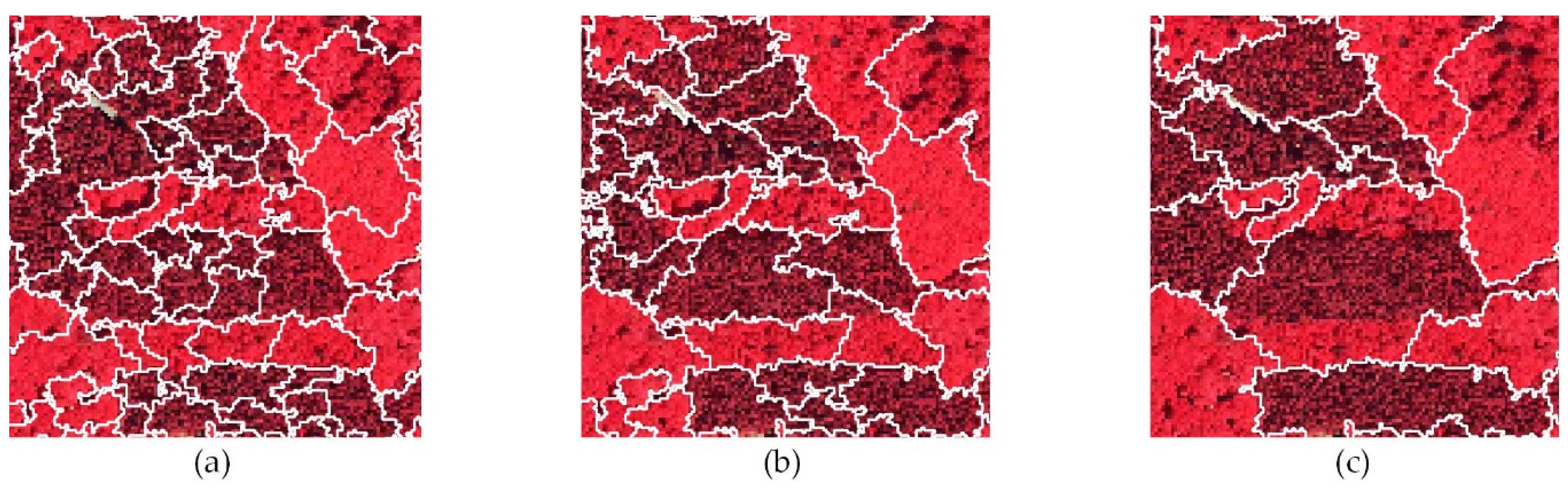
As the optimal threshold for segmentation was derived by the unsupervised parameter optimization approach, a plot of the F-measure based on the segmentation of nIR-aerial imagery can be investigated in Figure 5. The plot shows the value of the F-measure based on scaled intra-segment homogeneity and inter-segment heterogeneity for segmentations using different thresholds. Taking a look at forest area No. 4 again, the F-measure plot shows the best segmentation could be derived with a threshold of 0.46. In Figure 6, close-ups of segmentation derived by the optimal threshold, by a lower threshold (0.44) and on a higher threshold (0.49) can be compared. Figure 6b shows that the optimal threshold for segmentation is also visually well suited for the task of forest stratification based on leaf type. Additionally, the lower threshold shows that oversegmentation is not necessarily a criterion to dismiss a segmentation as visually it compares well with the segmentation from the optimal threshold. In Figure 6c on the other hand, the segmentation result of the higher threshold shows undersegmentation, resulting in broadleaved and needleleaved stands that have not been well separated.
4.2. Classification and Validation
Classification of the derived segments has been carried out with a Random forest classifier in R using the Caret package. Different training setups (automatic and manual) and available features (with mean and standard deviation for radiometric features (RGB+nIR) and mean for textural features (Texture)) have been used to train the models to derive their impact on internal model accuracy. Models built on RGB features lead to the lowest model accuracies (70% automatic, 77% manual), while inclusion of the near Infrared leads to higher model accuracies, especially in the manual training setup (78% automatic, 91% manual). The inclusion of the texture features leads to higher accuracies in all setups (2–6%), while leading to the highest increase for the manual RGB setup (6%). Variable importance plots for each training setup using all features (RGB+nIR+Texture) additionally confirm the importance of the inclusion of nIR information as well as the texture measures (Figure 7).
Subsequently, models trained on RGB and RGB+Texture were used to classify the segments derived from RGB aerial imagery, while the segments derived from RGBnIR aerial imagery have been classified with the models trained with the inclusion of the nIR band (see Table 2). Classification accuracies derived through confusion matrices show the same pattern for each training setup, where the inclusion of texture measures increases the accuracy slightly. Comparison of accuracies between the training setups show that classifications based on the automatic training setup reach slightly higher accuracies based on segments derived from RGB aerial imagery, while the manual training setup reaches higher accuracies based on segments derived from RGBnIR aerial imagery.
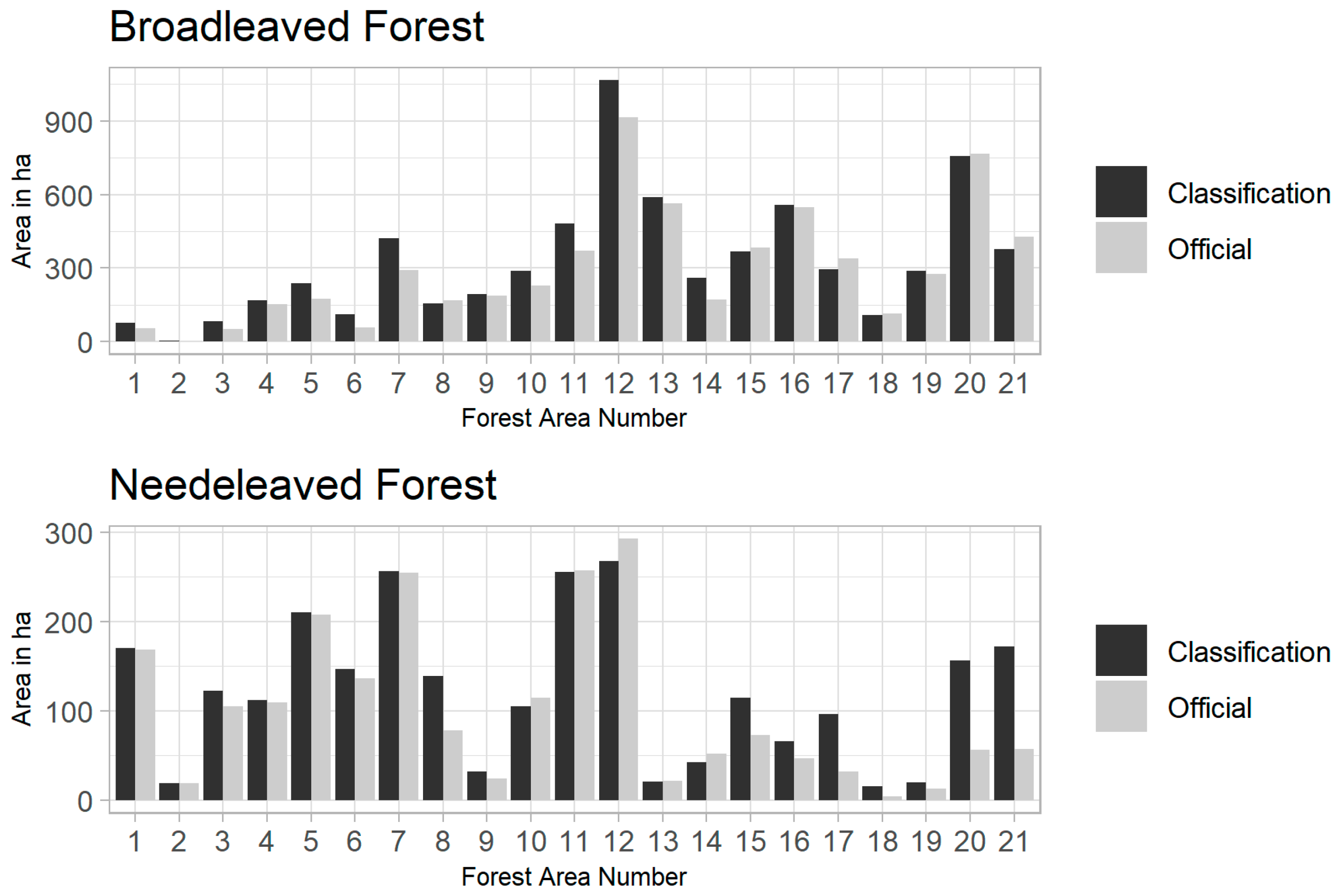
According to the best performing forest type classification (RGB+nIR+Texture) with an overall accuracy of 85%, the selected OSM mixed forest areas comprise 70 km2 of broadleaved and 26 km2 of needleleaved forest in total. Figure 8 shows size comparisons for broadleaved and needleleaved forest areas between classification and the official carto-/topographic database for each selected OSM forest area (compared with Figure 3). The comparison shows good agreement for many of the selected forest areas. The tendency of higher values for areas derived from the classification stems from mixed forest areas in the official carto-/topographic database. Since there is no mixed class in the classification procedure, the area that would be mixed forest in the official database is redistributed to broadleaved and needleleaved forest in the classification. Some of the selected forest areas are chosen to be investigated in more detail, i.e., forest area number 10 showing good agreement and forest area number 8 showing good agreement in the broadleaved class, but large overestimation of the needleleaved class. This is also reflected by the classification accuracies for these particular areas, where forest area number 10 reaches an overall accuracy of 92% while forest area number 8 reaches only 74% overall accuracy.
The best performing classifications (manual training with RGB+nIR+Texture) have been chosen for a closer look. Table 3 shows the confusion matrix of the classification with additional information on class accuracies (producer’s and user’s accuracies) and indication of quantity and allocation disagreement in addition to overall accuracy and kappa statistic.
Figure 9 shows a spatial comparison of forest types from the official carto-/topographic database and the best performing classification result for forest area number 10. The classification has generally been successful to derive the correct forest types inside this particular OSM relation with good agreement to the forest types from the official carto-/topographic database as can be seen in the close-ups (blue and red box). It shows the workflow is able to delineate forest types in considerable detail. A closer look into these areas shows that the probability for the segments to belong to the broadleaved forest class is slightly over 50% in the red box close-up, while probabilities are much higher in the blue box close-up. This shows the model was not able to classify the segments in the red box with a high probability. The probability for needleleaved forest class is the remaining fraction to 1.
The result for forest area number 8 can be investigated in Figure 10. As indicated by the area comparison from Figure 8, the classification largely overestimated needleleaved forest in this forest area. Stands of broadleaved forest in the close-up have a low probability to belong to the broadleaved forest class, which might be due to a high proportion of shadows leading to lower spectral values and to confusion with needleleaved forest.
5. Discussion
The presented work demonstrates a stratification of forest types inside larger OSM forest polygons tagged with the leaf-type mixed. It could successfully be demonstrated that an open source and open data workflow is suitable to derive this stratification and that it leads to promising results which can further be built on. The workflow itself is easy to implement as the data and software needed is openly available and can be replicated where similar data sources are available. It can be assumed the workflow is transferable to other regions if high resolution imagery is available and a sufficient amount of forest areas are correctly tagged in the OSM database. Problematic aspects could be determined and improvements of the workflow need to be established for the approach to be developed further. Particular aspects will be highlighted in the following sections.
5.1. Separation of Forest Types Based on Region Growing Segmentation and Aerial Imagery inside Existing Vector Boundaries
Segmentation is a critical processing step in GEOBIA workflows, strongly influencing the possible accuracy of the subsequent classification. The unsupervised parameter selection used to derive the best segmentation parameter has worked well and could visually be verified in most cases. Due to the results being specific for each of the selected forest area, very different thresholds might be selected as the best segmentation parameter. The approach assures that each forest area is segmented based on internal variations of the spectral values, but segmentations for different forest areas can thus not be easily compared. Subsequently, this approach can lead to very small segments in a quite uniform forest area. As uniform forest areas are further subdivided to small segments, the influence of some problematic aspects of the aerial images, like shadow cast, increases and leads to many misclassifications of shadows to needleleaved forest. Additional pre-processing of the aerial imagery using smoothing algorithms might be able to reduce the creation of segments which mainly contain shadow patches.
Concerning the input imagery, resampling to lower resolution (2 m × 2 m instead of 20 cm × 20 cm original resolution) has the advantage of tackling the segmentation problem at the intended scale. As the result should delineate homogenous forest patches and not individual tree crowns. In the same way, a resolution of 10 m would be sufficient to delineate larger forest patches and a resolution of 30 m and more could be used to delineate smaller landscape elements. Segmentation based on the original spatial resolution could be used to delineate individual tree crowns, especially with integration of data on crown height. Post-processing techniques would then be needed to group individual trees to derive forest patches.
Additionally, the use of a single-date aerial image might not be ideal if the aerial image of the target region has been derived in a period where broadleaved and needleleaved species are not well distinguishable. The inclusion of a near infrared band highly increases the quality of the segmentation as could be demonstrated. Possibilities to further improve the segmentation are inclusion of digital surface and elevation models and the integration of remote sensing datasets (i.e., Sentinel-2) to include temporal and phenological characteristics. The segmentation is presently evaluated on the input imagery bands, but selected bands or additionally calculated indices could be used in order to find the best segmentation parameter.
5.2. Classification of Derived Segments
As could be seen from the selection of training areas, the manual check of OSM forest polygons has led to a decrease in training polygons. These polygons included forest areas that do not contain forest cover in the aerial image of 2018 and forest areas with false tags, either large mixed forest polygons tagged as broadleaved/needleleaved or mix-ups of broadleaved and needleleaved forests. It was therefore expected that the manual training approach would subsequently lead to higher classification accuracies. This could be confirmed, but the automatic and manual training approaches lead to very similar classification accuracies, which might be explained by the still large amount of correctly tagged forest areas in the automatic approach and a larger sample size. The influence of the forests with false tags could be too low to have substantial influence on the training performance. Good results could be derived by training data being readily available for the study area of Luxembourg. This might not be the case for areas where land cover digitization is less prominent or where forests are tagged as mixed in their entirety.
As presented in Figure 10 for forest area 8, the best performing classification still led to misclassifications of forest areas that are easily distinguishable visually, even if the segmentation led to a good result. This indicates the model for classification should further be improved. The class accuracy measures (Table 3), indicate remaining problems with the classification, especially with needleleaved forest being the minority class. There are several reasons for misclassifications that could be identified for official needleleaved forest classified as broadleaved forest:
- General stand border situations.
- Border situations with mixed forest.
- New growth needleleaved forests.
- Under-/Oversegmentation of structurally rich forest areas.
Problems with misclassifications of official broadleaved forests classified as needleleaved forests are mainly due to high shadow proportion in open stand conditions. This could be solved by the inclusion of a shadow class, but questions remain on how to handle the class for the final forest map, as it does not give any thematic information. Other options should be explored, as i.e., Chen et al. (2011) [14] used shadow fraction as additional input feature for classification of derived segments.
5.3. Upgrade of OpenStreetMap Geometries through Spatial and Thematic Subdivisions of Leaf Type
Concerning the presented approach, a reintegration of spatial and thematic subdivisions of forest areas could not be achieved as the results of the previous processing steps need to be improved to achieve a higher quality. Further developing the methodology might lead to subdivisions of forest type fit to be integrated to OSM. Given a higher quality of subdivisions, a reintegration to OpenStreetMap should include the involvement from OSM contributors. Trying to find strategies to reintegrate the results back into the OSM database, a verification of OSM contributors might be a promising approach. New approaches on data acquisition for OSM focus i.e., on AI-detected roads, which need to be verified by OSM contributors to finally be included in the OSM database. Therefore, a possibility would be to set up a project dedicated to invite contributors to identify and verify the detected leaf type for subdivided forest areas. On the other hand, the presented methodology could also be integrated in a scenario where regions with additional leaf-type content are indicated to guide contributors to areas where detailed digitization of forest types would result in a spatial and thematic update of the OSM database. An option for the presented approach would be to post-process only those segments with high class probabilities for one of the forest type classes and integrate those areas back into the OpenStreetMap database. Areas of low probabilities would remain as leaf-type mixed forest polygons. In any case, a strategy to integrate the resulting segments into OSM has to be found and needs to follow the OSM importing guidelines.
6. Conclusions
The resulting stratification demonstrates the derivation of forest type maps from OSM would be feasible with an extended and improved methodology. The use of OSM-geometry in combination with remote sensing data and methods might be able to provide valuable contributions to the information need of accurate forest type maps. It also suggests an improved methodology might be able to provide updates of leaf type to the OSM database with contributor participation. However, questions remain as technical aspects in order to reintegrate the data into the OSM database have not been discussed in detail. The presented approach only comes to its full potential given the high quality of OSM contributions, covering a substantial amount of the investigated area to be able to derive training data. OSM Forests in Luxembourg are well digitized and are being updated regularly. It is also to show the potential arising from opening state-funded datasets to the public and to integrate different data sources for the best possible outcome. Concerning this, several open datasets remain untouched in the present study and much potential still needs to be investigated (i.e., Sentinel-2 to derive phenological information, incorporation of the digital elevation and surface models).
Integration of OSM into remote sensing workflows has a large potential to create, update, upgrade and spatialize forest type maps. We could contribute a first look into this direction and promising first results could be achieved. According to the results, the research question has to be answered in a more differentiated way. Is it possible to use OSM data and aerial imagery to create, upgrade, update and spatialize forest type maps? OSM can be used to create a forest type map where contribution is high and where areas are present that are correctly tagged with their leaf types or can further be subdivided to derive leaf types. To derive a forest type map for whole Luxembourg, all mixed forest areas need to be processed and evaluated, broadleaved and needleleaved forest areas need to be checked for correct leaf types and present forest cover and additional areas with tags like natural=wood, leisure=park, etc., would need to be included. The workflow that was presented is based on open source software and open data, is easy to implement and can be transferred and reproduced in other regions. Upgrade and update of the OSM forest types could at present not be achieved as the resulting classifications are not of a quality that would allow a reintegration into the OSM database. Further improvement of this workflow could result in a stratification of forest types which could then be confirmed by contributors before being integrated into the OSM database.
Author Contributions
Conceptualization, Melanie Brauchler and Johannes Stoffels; Data curation, Melanie Brauchler; Formal analysis, Melanie Brauchler; Investigation, Melanie Brauchler and Johannes Stoffels; Methodology, Melanie Brauchler and Johannes Stoffels; Project administration, Melanie Brauchler and Johannes Stoffels; Resources, Melanie Brauchler; Software, Melanie Brauchler; Supervision, Johannes Stoffels; Validation, Melanie Brauchler; Visualization, Melanie Brauchler; writing—original draft, Melanie Brauchler; writing—review and editing, Melanie Brauchler and Johannes Stoffels. All authors have read and agreed to the published version of the manuscript.
Funding
The publication was funded by the Open Access Fund of Universität Trier and the German Research Foundation (DFG) within the Open Access Publishing funding programme.
Acknowledgments
The authors would like to thank all OpenStreetMap contributors, GRASS GIS and R developers for their invaluable contributions. The authors are also grateful to Ryan O’Leary and Esra Bohlender (Trier University) who helped proof-reading the transcript. We are also thankful for and appreciate the suggestions of three anonymous reviewers that helped us to improve our work.
Conflicts of Interest
The authors declare no conflict of interest.
References
- Liu, Y.; Gong, W.; Hu, X.; Gong, J. Forest Type Identification with Random Forest Using Sentinel-1A, Sentinel-2A, Multi-Temporal Landsat-8 and DEM Data. Remote Sens. 2018, 10, 946. [Google Scholar] [CrossRef] [Green Version]
- Pasquarella, V.J.; Holden, C.E.; Woodcock, C.E. Improved mapping of forest type using spectral-temporal Landsat features. Remote Sens. Environ. 2018, 210, 193–207. [Google Scholar] [CrossRef]
- Nink, S.; Hill, J.; Stoffels, J.; Buddenbaum, H.; Frantz, D.; Langshausen, J. Using Landsat and Sentinel-2 Data for the Generation of Continuously Updated Forest Type Information Layers in a Cross-Border Region. Remote Sens. 2019, 11, 2337. [Google Scholar] [CrossRef] [Green Version]
- Zhu, X.; Liu, D. Accurate mapping of forest types using dense seasonal Landsat time-series. ISPRS J. Photogramm. Remote Sens. 2014, 96, 1–11. [Google Scholar] [CrossRef]
- Kempeneers, P.; Sedano, F.; Seebach, L.; Strobl, P.; San-Miguel-Ayanz, J. Data fusion of different spatial resolution remote sensing images applied to forest-type mapping. IEEE Trans. Geosci. Remote Sens. 2011, 49, 4977–4986. [Google Scholar] [CrossRef]
- Stoffels, J.; Hill, J.; Sachtleber, T.; Mader, S.; Buddenbaum, H.; Stern, O.; Langshausen, J.; Dietz, J.; Ontrup, G. Satellite-Based Derivation of High-Resolution Forest Information Layers for Operational Forest Management. Forests 2015, 6, 1982–2013. [Google Scholar] [CrossRef]
- Gillis, M.; Leckie, D. Forest Inventory Mapping Procedures across Canada. For. Chron. 1993, 71, 74–88. [Google Scholar]
- Tuominen, S.; Pekkarinen, A. Performance of different spectral and textural aerial photograph features in multi-source forest inventory. Remote Sens. Environ. 2005, 94, 256–268. [Google Scholar] [CrossRef]
- Hall, R.J. The roles of aerial photographs in forestry remote sensing image analysis. In Remote Sensing of Forest Environments; Springer: Boston, MA, USA, 2003; pp. 47–75. [Google Scholar]
- Lausch, A.; Erasmi, S.; King, D.; Magdon, P.; Heurich, M. Understanding Forest Health with Remote Sensing-Part I—A Review of Spectral Traits, Processes and Remote-Sensing Characteristics. Remote Sens. 2016, 8, 1029. [Google Scholar] [CrossRef] [Green Version]
- Chen, G.; Weng, Q.; Hay, G.J.; He, Y. Geographic object-based image analysis (GEOBIA): Emerging trends and future opportunities. Gisci. Remote Sens. 2018, 55, 159–182. [Google Scholar] [CrossRef]
- Smith, G.M.; Morton, R.D. Real world objects in GEOBIA through the exploitation of existing digital cartography and image segmentation. Photogramm. Eng. Remote Sens. 2010, 76, 163–171. [Google Scholar] [CrossRef]
- Kim, M.; Warner, T.A.; Madden, M.; Atkinson, D.S. Multi-scale GEOBIA with very high spatial resolution digital aerial imagery: Scale, texture and image objects. Int. J. Remote Sens. 2011, 32, 2825–2850. [Google Scholar] [CrossRef]
- Chen, G.; Hay, G.J.; Castilla, G.; St-Onge, B.; Powers, R. A multiscale geographic object-based image analysis to estimate lidar-measured forest canopy height using Quickbird imagery. Int. J. Geogr. Inf. Sci. 2011, 25, 877–893. [Google Scholar] [CrossRef]
- Lang, S.; Hay, G.J.; Baraldi, A.; Tiede, D.; Blaschke, T. Geobia Achievements and Spatial Opportunities in the Era of Big Earth Observation Data. ISPRS Int. J. Geo-Inf. 2019, 8, 474. [Google Scholar] [CrossRef] [Green Version]
- Kim, M.; Madden, M.; Warner, T.A. Forest type mapping using object-specific texture measures from multispectral Ikonos imagery. Photogramm. Eng. Remote Sens. 2009, 75, 819–829. [Google Scholar] [CrossRef] [Green Version]
- Blaschke, T.; Hay, G.J.; Kelly, M.; Lang, S.; Hofmann, P.; Addink, E.; Feitosa, R.Q.; Van der Meer, F.; Van der Werff, H.; Van Coillie, F. Geographic object-based image analysis–towards a new paradigm. ISPRS J. Photogramm. Remote Sens. 2014, 87, 180–191. [Google Scholar] [CrossRef] [Green Version]
- Hay, G.J.; Castilla, G. Geographic Object-Based Image Analysis (GEOBIA): A new name for a new discipline. In Object-Based Image Analysis; Springer: Berlin/Heidelberg, Germany, 2008; pp. 75–89. [Google Scholar]
- Yu, Q.; Gong, P.; Clinton, N.; Biging, G.; Kelly, M.; Schirokauer, D. Object-based detailed vegetation classification with airborne high spatial resolution remote sensing imagery. Photogramm. Eng. Remote Sens. 2006, 72, 799–811. [Google Scholar] [CrossRef] [Green Version]
- Aggarwal, N.; Srivastava, M.; Dutta, M. Comparative analysis of pixel-based and object-based classification of high resolution remote sensing images—A review. Int. J. Eng. Trends Technol. 2016, 38, 5–11. [Google Scholar] [CrossRef]
- Smith, G.; Morton, D. Segmentation: The Achilles’ heel of object–based image analysis? ISPRS Int. Arch. Photogramm. Remote Sens. Spat. Inf. Sci. 2008, 38, XXXVIII-4/C1. [Google Scholar]
- Gu, H.; Li, H.; Yan, L.; Lu, X. A framework for Geographic Object-Based Image Analysis (GEOBIA) based on geographic ontology. ISPRS Int. Arch. Photogramm. Remote Sens. Spat. Inf. Sci. 2015, 40, 27–33. [Google Scholar] [CrossRef] [Green Version]
- Griffith, D.; Hay, G. Integrating GEOBIA, Machine Learning, and Volunteered Geographic Information to Map Vegetation over Rooftops. ISPRS Int. J. Geo-Inf. 2018, 7, 462. [Google Scholar] [CrossRef] [Green Version]
- Mason, D.C.; Corr, D.; Cross, A.; Hogg, D.C.; Lawrence, D.; Petrou, M.; Tailor, A. The use of digital map data in the segmentation and classification of remotely-sensed images. Int. J. Geogr. Inf. Syst. 1988, 2, 195–215. [Google Scholar] [CrossRef]
- Sui, D.; Goodchild, M.; Elwood, S. Volunteered geographic information, the exaflood, and the growing digital divide. In Crowdsourcing Geographic Knowledge; Springer: Dordrecht, The Netherlands, 2013; pp. 1–12. [Google Scholar]
- Goodchild, M.F. Citizens as sensors: The world of volunteered geography. GeoJournal 2007, 69, 211–221. [Google Scholar] [CrossRef] [Green Version]
- Ballatore, A.; Bertolotto, M.; Wilson, D.C. Geographic knowledge extraction and semantic similarity in OpenStreetMap. Knowl. Inf. Syst. 2012, 37, 61–81. [Google Scholar] [CrossRef] [Green Version]
- Brovelli, M.A.; Wu, H.; Minghini, M.; Molinari, M.E.; Kilsedar, C.E.; Zheng, X.; Shu, P.; Chen, J. Open Source Software and Open Educational Material on Land Cover Maps Intercomparison and Validation. ISPRS Int. Arch. Photogramm. Remote Sens. Spat. Inf. Sci. 2018, 42, 61–68. [Google Scholar] [CrossRef] [Green Version]
- Pourabdollah, A.; Morley, J.; Feldman, S.; Jackson, M. Towards an Authoritative OpenStreetMap: Conflating OSM and OS OpenData National Maps’ Road Network. ISPRS Int. J. Geo-Inf. 2013, 2, 704–728. [Google Scholar] [CrossRef]
- Mooney, P.; Corcoran, P. Has OpenStreetMap a role in Digital Earth applications? Int. J. Digit. Earth 2013, 7, 534–553. [Google Scholar] [CrossRef] [Green Version]
- Barron, C.; Neis, P.; Zipf, A. A Comprehensive Framework for Intrinsic OpenStreetMap Quality Analysis. Trans. GIS 2014, 18, 877–895. [Google Scholar] [CrossRef]
- Zilske, M.; Neumann, A.; Nagel, K. OpenStreetMap for Traffic Simulation; Technische Universität Berlin: Berlin, Germany, 2015. [Google Scholar]
- Zhao, P.; Jia, T.; Qin, K.; Shan, J.; Jiao, C. Statistical analysis on the evolution of OpenStreetMap road networks in Beijing. Phys. A Stat. Mech. Its Appl. 2015, 420, 59–72. [Google Scholar] [CrossRef]
- Zhang, Y.; Li, X.; Wang, A.; Bao, T.; Tian, S. Density and diversity of OpenStreetMap road networks in China. J. Urban Manag. 2015, 4, 135–146. [Google Scholar] [CrossRef] [Green Version]
- Luxen, D.; Vetter, C. Real-time routing with OpenStreetMap data. In Proceedings of the 19th ACM SIGSPATIAL International Conference on Advances in Geographic Information Systems, Chicago, IL, USA, 1–4 November 2011; pp. 513–516. [Google Scholar]
- Fan, H.; Zipf, A.; Fu, Q. Estimation of building types on OpenStreetMap based on urban morphology analysis. In Connecting a Digital Europe through Location and Place; Springer: Cham, Switzerland, 2014; pp. 19–35. [Google Scholar]
- Bakillah, M.; Liang, S.; Mobasheri, A.; Jokar Arsanjani, J.; Zipf, A. Fine-resolution population mapping using OpenStreetMap points-of-interest. Int. J. Geogr. Inf. Sci. 2014, 28, 1940–1963. [Google Scholar] [CrossRef]
- Estima, J.; Painho, M. Investigating the potential of OpenStreetMap for land use/land cover production: A case study for continental Portugal. In OpenStreetMap in GIScience; Springer: Cham, Switzerland, 2015; pp. 273–293. [Google Scholar]
- Fonte, C.C.; Patriarca, J.A.; Minghini, M.; Antoniou, V.; See, L.; Brovelli, M.A. Using openstreetmap to create land use and land cover maps: Development of an application. In Geospatial Intelligence: Concepts, Methodologies, Tools, and Applications; IGI Global: Hershey, PA, USA, 2019; pp. 1100–1123. [Google Scholar]
- Arsanjani, J.J.; Mooney, P.; Zipf, A.; Schauss, A. Quality assessment of the contributed land use information from OpenStreetMap versus authoritative datasets. In OpenStreetMap in GIScience; Springer: Cham, Switzerland, 2015; pp. 37–58. [Google Scholar]
- Schultz, M.; Voss, J.; Auer, M.; Carter, S.; Zipf, A. Open land cover from OpenStreetMap and remote sensing. Int. J. Appl. Earth Obs. Geoinf. 2017, 63, 206–213. [Google Scholar] [CrossRef]
- Yang, D.; Fu, C.-S.; Smith, A.C.; Yu, Q. Open land-use map: A regional land-use mapping strategy for incorporating OpenStreetMap with earth observations. Geo-Spat. Inf. Sci. 2017, 20, 269–281. [Google Scholar] [CrossRef] [Green Version]
- Yang, D. Mapping Regional Landscape by Using OpenstreetMap (OSM). In Environmental Information Systems: Concepts, Methodologies, Tools, and Applications; IGI Global: Hershey, PA, USA, 2019; pp. 771–790. [Google Scholar] [CrossRef]
- Upton, V.; Ryan, M.; O’Donoghue, C.; Dhubhain, A.N. Combining conventional and volunteered geographic information to identify and model forest recreational resources. Appl. Geogr. 2015, 60, 69–76. [Google Scholar] [CrossRef]
- Grippa, T.; Georganos, S.; Vanhuysse, S.; Lennert, M.; Mboga, N.; Wolff, É. Mapping slums and model population density using earth observation data and open source solutions. In Proceedings of the 2019 Joint Urban Remote Sensing Event (JURSE), Vannes, France, 22–24 May 2019; pp. 1–4. [Google Scholar]
- Liu, C.; Xiong, L.; Hu, X.; Shan, J. A progressive buffering method for road map update using OpenStreetMap data. ISPRS Int. J. Geo-Inf. 2015, 4, 1246–1264. [Google Scholar] [CrossRef] [Green Version]
- Rondeux, J.; Alderweireld, M.; Saidi, M.; Schillings, T.; Freymann, E.; Murat, D.; Kugener, G. La Forêt Luxembourgeoise en Chiffres-Résultats de l’Lnventaire Forestier National au Grand-Duché de Luxembourg 2009–2011; Administration de la Nature et des forêts du Grand-Duché de Luxembourg—Service des Forêts: Diekirch, Luxembourg, 2014.
- Niemeyer, T.; Härdtle, W.; Ries, C. Die Waldgesellschaften Luxemburgs: Vegetation, Standort, Vorkommen und Gefährdung; Musée National D’Histoire Naturelle Luxembourg: Luxembourg, 2010. [Google Scholar]
- BD-L-TC-forests from the Official Carto-/Topographic Database. Available online: https://data.public.lu/fr/datasets/bd-l-tc-2015/ (accessed on 20 December 2019).
- Photos Aériennes. Available online: https://act.public.lu/fr/cartographie/photos-aeriennes.html (accessed on 22 July 2020).
- Orthophoto Officelle du Grand-Duché de Luxembourg, Édition 2018. Available online: https://data.public.lu/fr/datasets/orthophoto-officelle-du-grand-duche-de-luxembourg-edition-2018/ (accessed on 10 November 2019).
- Raifer, M. Overpass Turbo—Overpass API. Available online: http://overpass-turbo.eu/ (accessed on 15 January 2020).
- Bins, L.S.; Fonseca, L.G.; Erthal, G.J.; Ii, F.M. Satellite imagery segmentation: A region growing approach. Simpósio Bras. De Sens. Remoto 1996, 8, 677–680. [Google Scholar]
- Räsänen, A.; Kuitunen, M.; Tomppo, E.; Lensu, A. Coupling high-resolution satellite imagery with ALS-based canopy height model and digital elevation model in object-based boreal forest habitat type classification. ISPRS J. Photogramm. Remote Sens. 2014, 94, 169–182. [Google Scholar] [CrossRef] [Green Version]
- Räsänen, A.; Rusanen, A.; Kuitunen, M.; Lensu, A. What makes segmentation good? A case study in boreal forest habitat mapping. Int. J. Remote Sens. 2013, 34, 8603–8627. [Google Scholar] [CrossRef]
- Momsen, E.; Metz, M.; GRASS Development Team. Available online: https://grass.osgeo.org/grass76/manuals/addons/i.segment.gsoc.html (accessed on 5 March 2020).
- Benz, U.C.; Hofmann, P.; Willhauck, G.; Lingenfelder, I.; Heynen, M. Multi-resolution, object-oriented fuzzy analysis of remote sensing data for GIS-ready information. ISPRS J. Photogramm. Remote Sens. 2004, 58, 239–258. [Google Scholar] [CrossRef]
- Grippa, T.; Lennert, M.; Beaumont, B.; Vanhuysse, S.; Stephenne, N.; Wolff, E. An Open-Source Semi-Automated Processing Chain for Urban Object-Based Classification. Remote Sens. 2017, 9, 358. [Google Scholar] [CrossRef] [Green Version]
- Espindola, G.; Câmara, G.; Reis, I.; Bins, L.; Monteiro, A. Parameter selection for region-growing image segmentation algorithms using spatial autocorrelation. Int. J. Remote Sens. 2006, 27, 3035–3040. [Google Scholar] [CrossRef]
- Johnson, B.A.; Bragais, M.; Endo, I.; Magcale-Macandog, D.B.; Macandog, P.B.M. Image segmentation parameter optimization considering within-and between-segment heterogeneity at multiple scale levels: Test case for mapping residential areas using landsat imagery. ISPRS Int. J. Geo-Inf. 2015, 4, 2292–2305. [Google Scholar] [CrossRef] [Green Version]
- Carleer, A.; Debeir, O.; Wolff, E. Assessment of very high spatial resolution satellite image segmentations. Photogramm. Eng. Remote Sens. 2005, 71, 1285–1294. [Google Scholar] [CrossRef] [Green Version]
- UNFCCC. Report of the Conference of the Parties on Its Seventh Session, Held at Marrakesh from 29 October to 10 November 2001; FCCC/CP/2001/13/Add.1; UNFCCC: Marrakesh, Morocco, 2001. [Google Scholar]
- Mallinis, G.; Koutsias, N.; Tsakiri-Strati, M.; Karteris, M. Object-based classification using Quickbird imagery for delineating forest vegetation polygons in a Mediterranean test site. ISPRS J. Photogramm. Remote Sens. 2008, 63, 237–250. [Google Scholar] [CrossRef]
- Kim, M.; Madden, M.; Xu, B. GEOBIA vegetation mapping in Great Smoky Mountains National Park with spectral and non-spectral ancillary information. Photogramm. Eng. Remote Sens. 2010, 76, 137–149. [Google Scholar] [CrossRef]
- Haralick, R.M.; Shanmugam, K.; Dinstein, I.H. Textural features for image classification. IEEE Trans. Syst. ManCybern. 1973, 610–621. [Google Scholar] [CrossRef] [Green Version]
- Feng, Q.; Liu, J.; Gong, J. UAV remote sensing for urban vegetation mapping using random forest and texture analysis. Remote Sens. 2015, 7, 1074–1094. [Google Scholar] [CrossRef] [Green Version]
- Antoniol, G.; Basco, C.; Ceccarelli, M.; Metz, M.; Lennart, M.; GRASS Development Team. Available online: https://grass.osgeo.org/grass78/manuals/r.texture.html (accessed on 5 March 2020).
- Haralick, R.M. Statistical and structural approaches to texture. Proc. IEEE 1979, 67, 786–804. [Google Scholar] [CrossRef]
- Hall-Beyer, M. Practical guidelines for choosing GLCM textures to use in landscape classification tasks over a range of moderate spatial scales. Int. J. Remote Sens. 2017, 38, 1312–1338. [Google Scholar] [CrossRef]
- Breiman, L. Random forests. Mach. Learn. 2001, 45, 5–32. [Google Scholar] [CrossRef] [Green Version]
- Kuhn, M. Caret: Classification and Regression Training. Available online: https://CRAN.R-project.org/package=caret (accessed on 10 March 2019).
- Belgiu, M.; Drăguţ, L. Random forest in remote sensing: A review of applications and future directions. ISPRS J. Photogramm. Remote Sens. 2016, 114, 24–31. [Google Scholar] [CrossRef]
- Li, X.; Cheng, X.; Chen, W.; Chen, G.; Liu, S. Identification of Forested Landslides Using LiDar Data, Object-based Image Analysis, and Machine Learning Algorithms. Remote Sens. 2015, 7, 9705–9726. [Google Scholar] [CrossRef] [Green Version]
Figure 1.
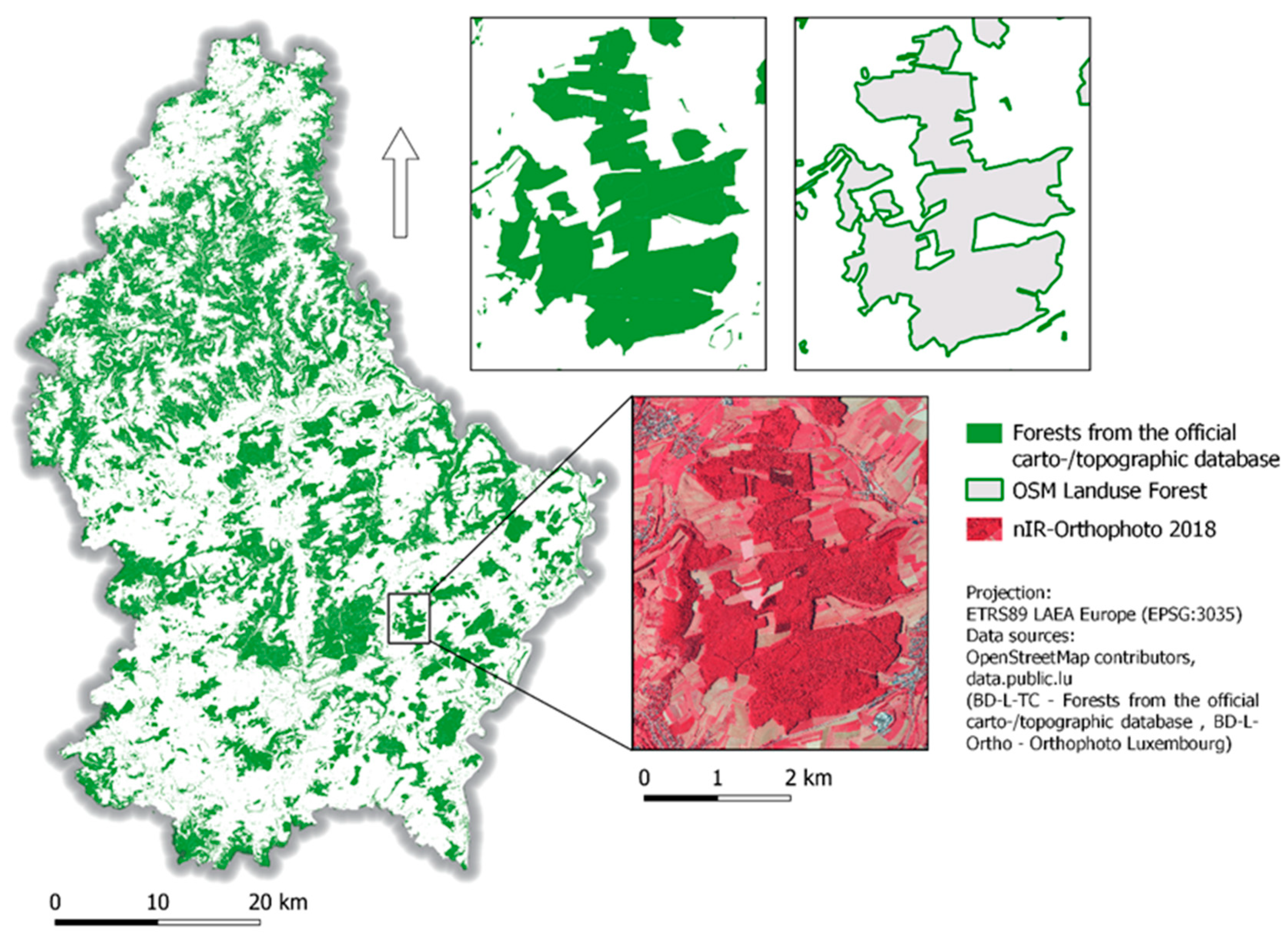
Overview of the forests from the official carto-/topographic database in the Grand Duchy of Luxembourg and close-ups of a forest area from the database compared to OSM Landuse Forest and the nIR-orthophoto from 2018.
Figure 1.
Overview of the forests from the official carto-/topographic database in the Grand Duchy of Luxembourg and close-ups of a forest area from the database compared to OSM Landuse Forest and the nIR-orthophoto from 2018.

Figure 2.
Schematic of the processing workflow.
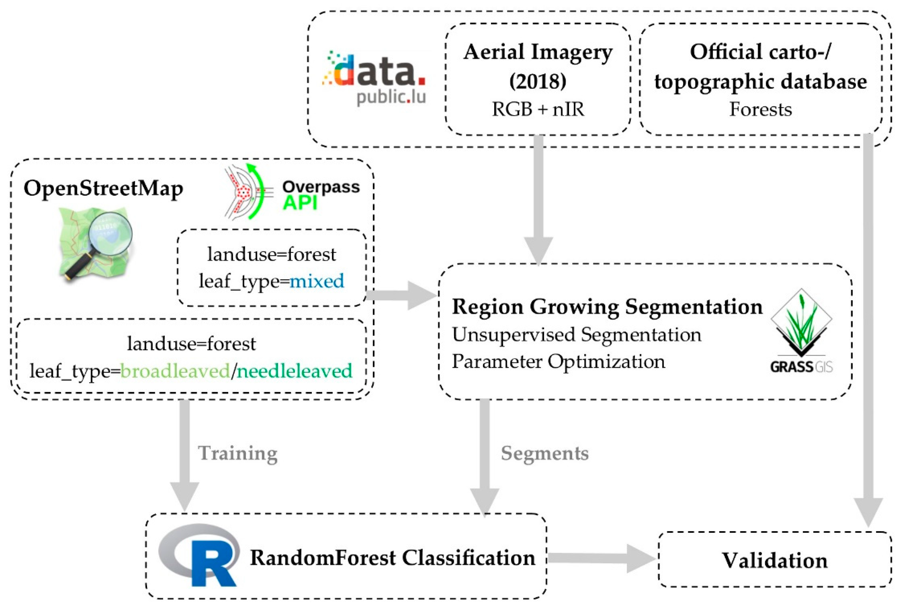
Figure 3.
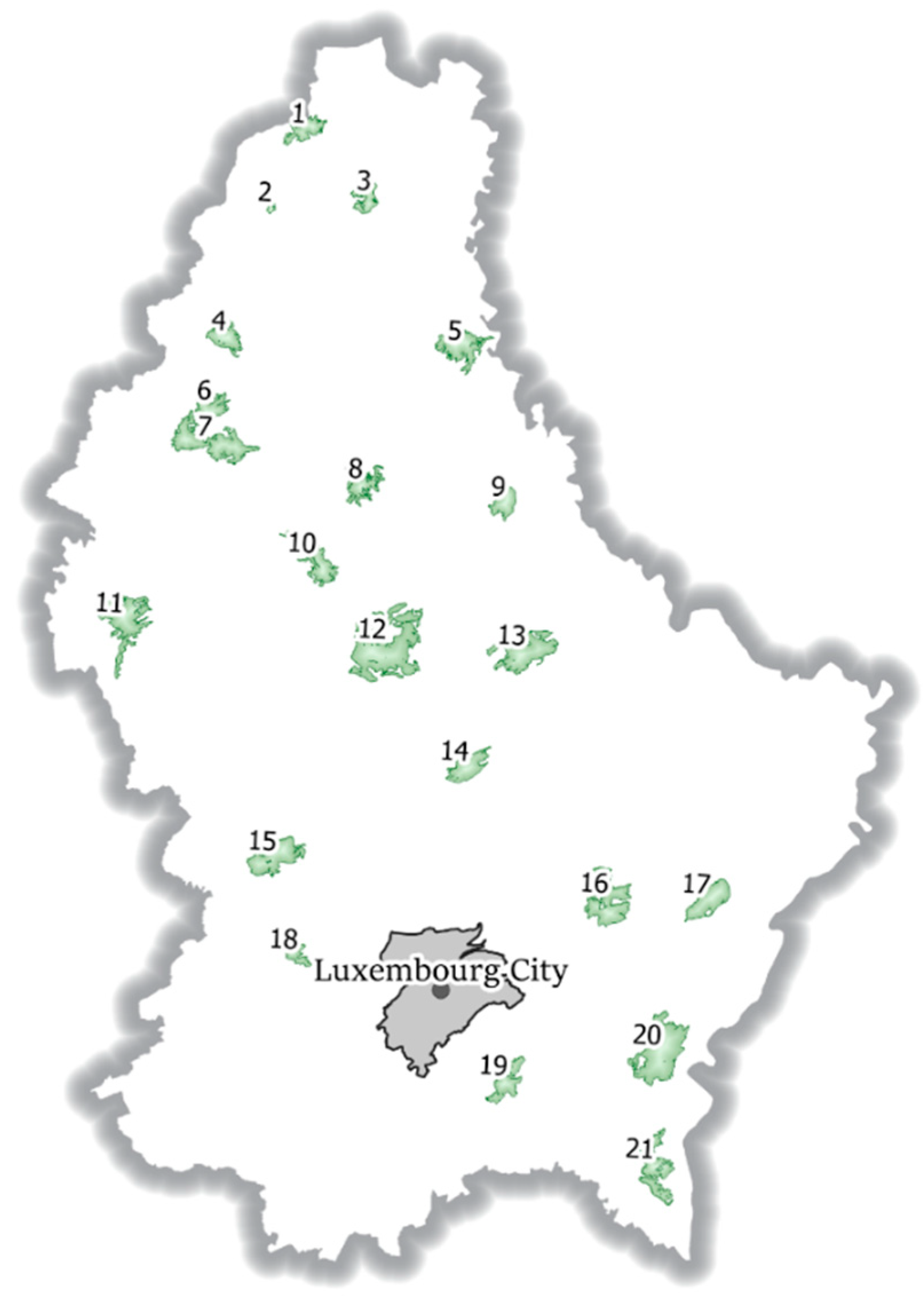
Selected OpenStreetMap (OSM) mixed forest polygons and their location in the Grand Duchy of Luxembourg.
Figure 3.
Selected OpenStreetMap (OSM) mixed forest polygons and their location in the Grand Duchy of Luxembourg.

Figure 4.
Results of the region growing segmentation on forest area No. 4. based on optimized thresholds (a) Overview of the segmentation based on RGB imagery with threshold 0.4; (b) Overview of the segmentation based on RGBnIR imagery with threshold 0.46; (c) Close-up of segmentation based on RGB imagery; (d) Close-up of segmentation on RGB imagery with RGB imagery in the background; (e) Close-up of segmentation on RGBnIR.
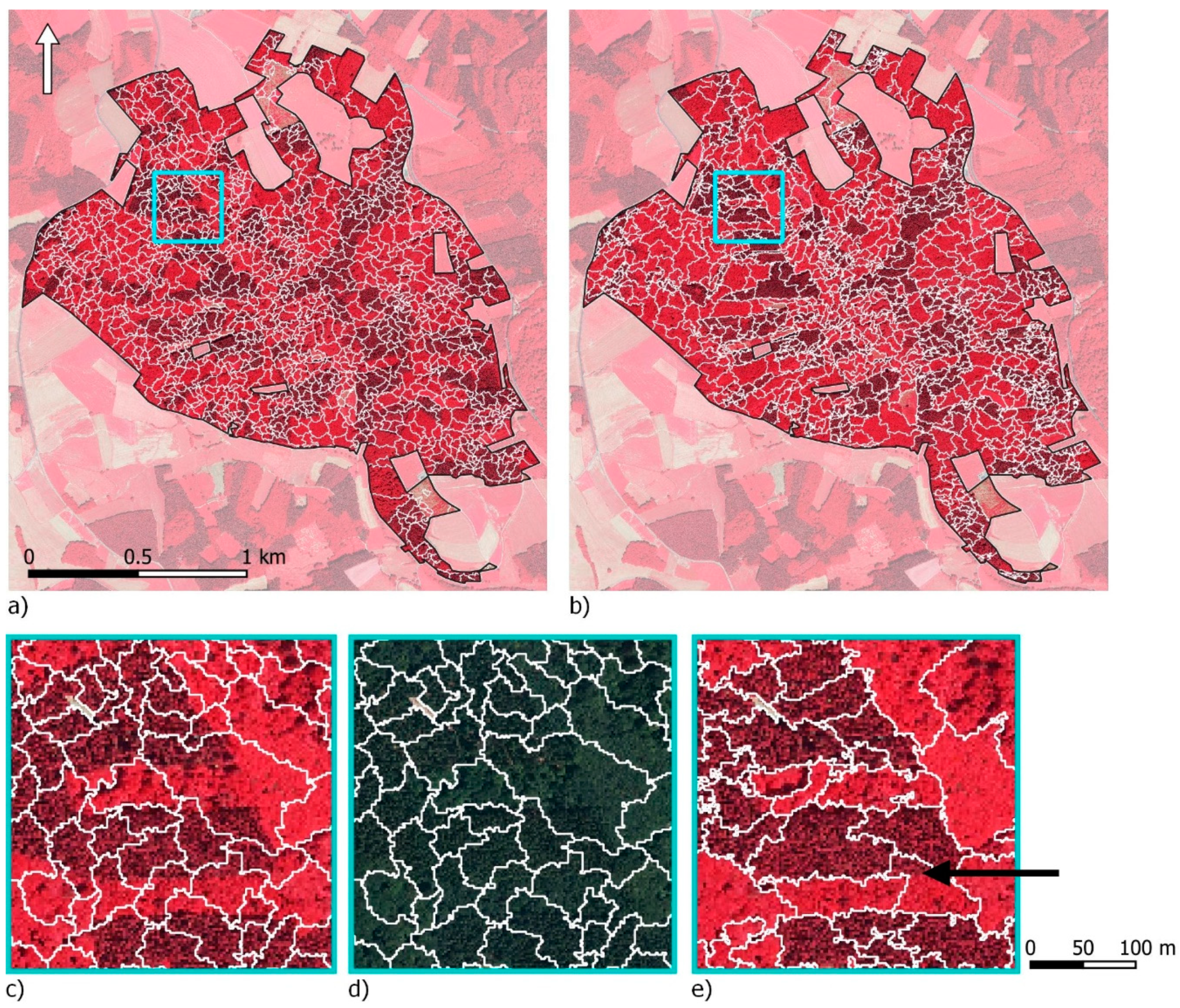
Figure 5.
F-Measure for selected OSM mixed forest polygons based on different thresholds. The dotted orange line indicates the optimal threshold for forest area No. 4.
Figure 5.
F-Measure for selected OSM mixed forest polygons based on different thresholds. The dotted orange line indicates the optimal threshold for forest area No. 4.
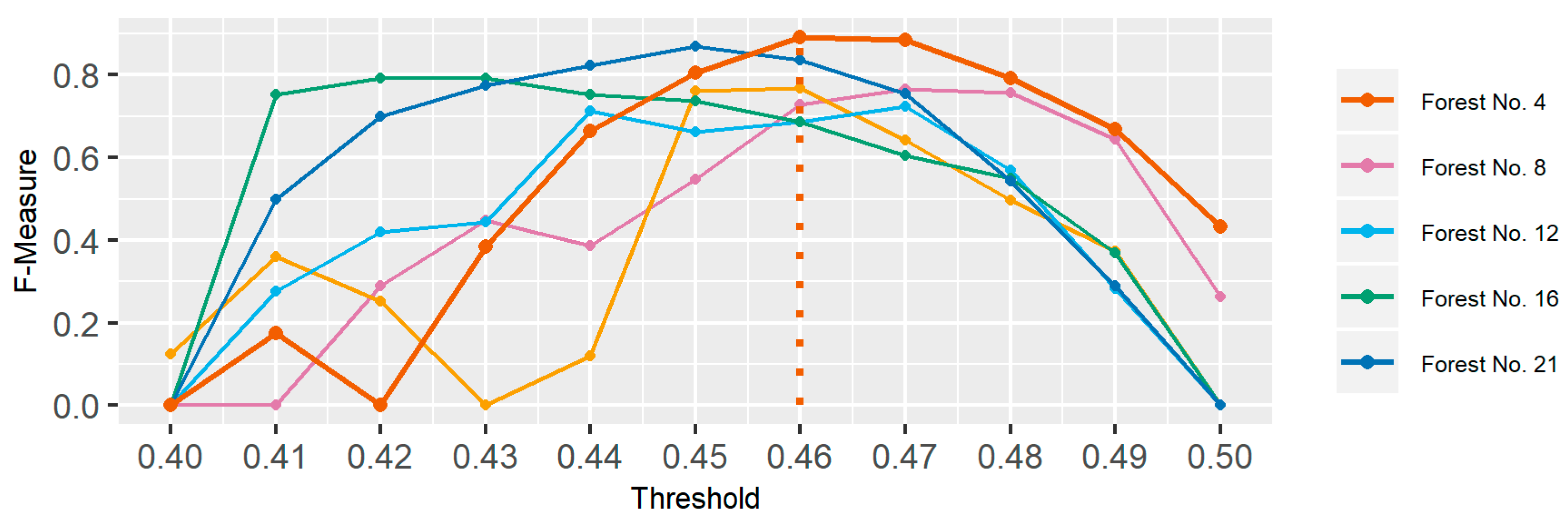
Figure 6.
Results of the region growing segmentation on forest area No. 4 on RGBnIR imagery with a threshold (a) 0.44; (b) 0.46 (optimal); (c) 0.49.
Figure 6.
Results of the region growing segmentation on forest area No. 4 on RGBnIR imagery with a threshold (a) 0.44; (b) 0.46 (optimal); (c) 0.49.

Figure 7.
Variable importance in Random Forest training with training data derived by (a) automatic; (b) manual selection processes for models trained on all variables (RGB+nIR+Texture).
Figure 7.
Variable importance in Random Forest training with training data derived by (a) automatic; (b) manual selection processes for models trained on all variables (RGB+nIR+Texture).
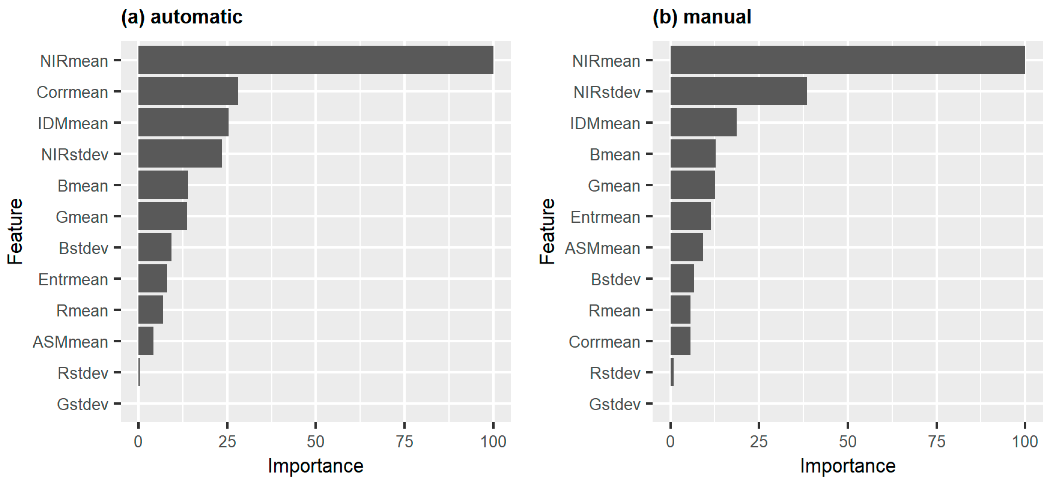
Figure 8.
Area comparison of the best performing forest type classification (Segmentation: RGB+nIR; Training: Manual; Input Features: RGB+nIR+texture) with the official carto-/topographic database for each selected forest area.
Figure 8.
Area comparison of the best performing forest type classification (Segmentation: RGB+nIR; Training: Manual; Input Features: RGB+nIR+texture) with the official carto-/topographic database for each selected forest area.

Figure 9.
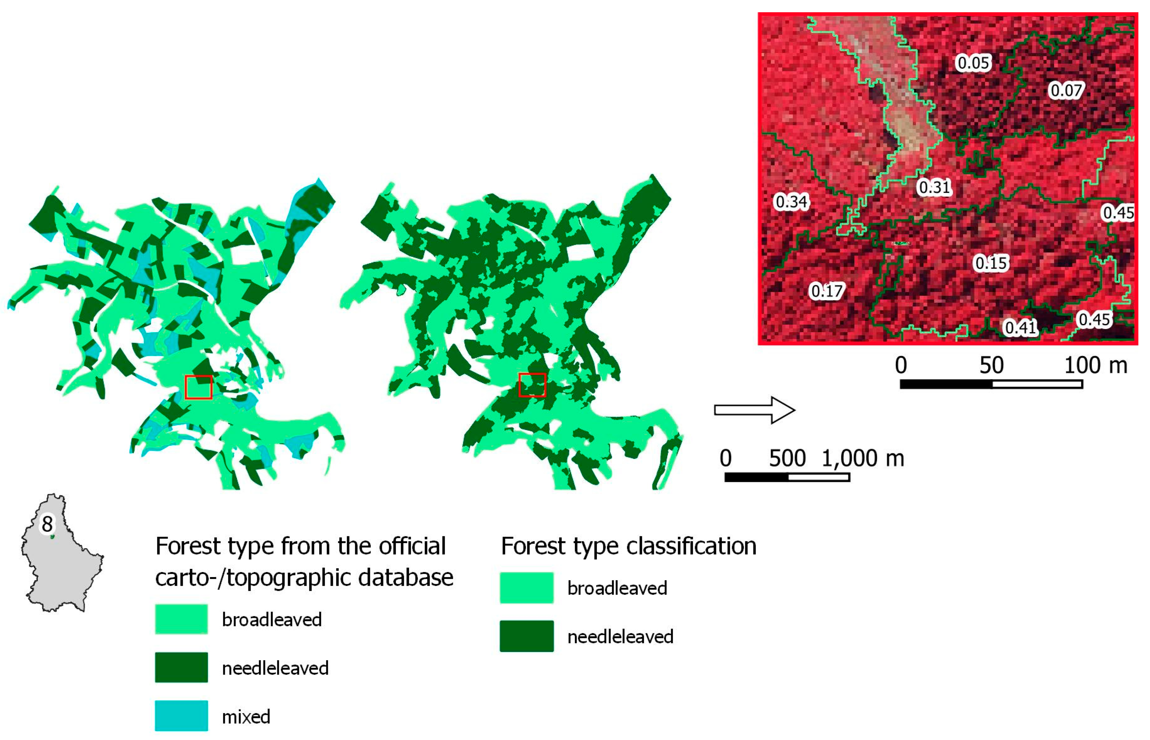
Comparison of forest types from the official carto-/topographic database with the best performing forest type classification for forest number 10 (Segmentation: RGB+nIR; Training: Manual; Input Features: RGB+nIR+texture) with close-ups to areas where stratification has been successful. Values indicate probability of the area to belong to broadleaved forest type class as derived from the randomForest model.
Figure 9.
Comparison of forest types from the official carto-/topographic database with the best performing forest type classification for forest number 10 (Segmentation: RGB+nIR; Training: Manual; Input Features: RGB+nIR+texture) with close-ups to areas where stratification has been successful. Values indicate probability of the area to belong to broadleaved forest type class as derived from the randomForest model.

Figure 10.
Comparison of forest types from the official carto-/topographic database with the best performing forest type classification for forest number 8 (Segmentation: RGB+nIR; Training: Manual; Input Features: RGB+nIR+texture) with a close-up of a highly problematic area. Values indicate probability of the area to belong to broadleaved forest type class as derived from the randomForest model.

Table 1.
Number of training polygons for respective leaf-type derived through automatic and manual selection from the OpenStreetMap database in Luxembourg.
Table 1.
Number of training polygons for respective leaf-type derived through automatic and manual selection from the OpenStreetMap database in Luxembourg.
| Leaf Type | Automatic | Manual |
|---|---|---|
| broadleaved | 1205 | 522 |
| needleleaved | 771 | 453 |
Table 2.
Classification accuracies and kappa coefficient using different input variables and training setups.
Table 2.
Classification accuracies and kappa coefficient using different input variables and training setups.
| Segmentation | ||||||
| RGB (n = 19,925) | RGB + nIR (n = 36,008) | |||||
| Input Variables | ||||||
| RGB | RGB + Texture | RGB + nIR | RGB + nIR + Texture | |||
| Training Setup | Automatic | Accuracy | 0.73 | 0.77 | 0.80 | 0.84 |
| Kappa | 0.41 | 0.46 | 0.51 | 0.60 | ||
| Manual | Accuracy | 0.71 | 0.73 | 0.83 | 0.85 | |
| Kappa | 0.38 | 0.41 | 0.57 | 0.62 | ||
Table 3.
Confusion matrix and derived accuracies for RGB+nIR+Texture classification under the manual training setup.
Table 3.
Confusion matrix and derived accuracies for RGB+nIR+Texture classification under the manual training setup.
| n = 33,742 | Reference | ||
|---|---|---|---|
| Classification | Broadleaved | Needleleaved | |
| Broadleaved | 22,284 | 2136 | |
| Needleleaved | 2899 | 6423 | |
| PAB: 0.88 | PAN: 0.75 | UAB:0.91 | UAN: 0.69 |
| OAA: 0.85 | κ: 0.61 | CAA: 0.82 | |
| Q: 0.02 A: 0.13 | |||
| OAA: Overall Accuracy; κ: Cohens Kappa CAA: Class-Averaged Accuracy; Q: Quantity Disagreement; A: Allocation Disagreement | |||
© 2020 by the authors. Licensee MDPI, Basel, Switzerland. This article is an open access article distributed under the terms and conditions of the Creative Commons Attribution (CC BY) license (http://creativecommons.org/licenses/by/4.0/).
Share and Cite
MDPI and ACS Style
Brauchler, M.; Stoffels, J. Leveraging OSM and GEOBIA to Create and Update Forest Type Maps. ISPRS Int. J. Geo-Inf. 2020, 9, 499. https://0-doi-org.brum.beds.ac.uk/10.3390/ijgi9090499
AMA Style
Brauchler M, Stoffels J. Leveraging OSM and GEOBIA to Create and Update Forest Type Maps. ISPRS International Journal of Geo-Information. 2020; 9(9):499. https://0-doi-org.brum.beds.ac.uk/10.3390/ijgi9090499
Chicago/Turabian StyleBrauchler, Melanie, and Johannes Stoffels. 2020. "Leveraging OSM and GEOBIA to Create and Update Forest Type Maps" ISPRS International Journal of Geo-Information 9, no. 9: 499. https://0-doi-org.brum.beds.ac.uk/10.3390/ijgi9090499
Note that from the first issue of 2016, this journal uses article numbers instead of page numbers. See further details here.