Analyzing the Influence of Urban Street Greening and Street Buildings on Summertime Air Pollution Based on Street View Image Data

Abstract

Transport emissions and street dust are important sources of summertime air pollution in urban centers. Street greening and buildings have an influence on the diffusion of air pollution from streets. For field measurements, many studies have analyzed the effect of street green space arrangement on the diffusion of air pollution, but these studies have neglected the patterns at the landscape scale. Other studies have analyzed the effects of the large scale of green space on air pollution, but the vertical distribution of street buildings and greening has rarely been considered. In this study, we analyzed the impact of the vertical distribution of urban street green space on summertime air pollution in urban centers on the urban scale for the first time by using a deep-learning method to extract the vertical distribution of street greening and buildings from street view image data. A total of 687,354 street view images were collected. The green index and building index were proposed to quantify the street greening and street buildings. The multilevel regression method was used to analyze the association between the street green index, building index and air pollution indexes. For the cases in this study, including the central urban areas of Beijing, Shanghai and Nanjing, our multilevel regressions results suggested that, in the central area of the city, the vertical distribution of street greening and buildings within a certain range of the monitoring site is association with the summertime air pollution index of the monitoring site. There was a significant negative association between the street greening and air pollution indexes (radius = 1–2 km, NO₂, p = 0.042; radius = 3–4 km, AQI, p = 0.034; PM₁₀, p = 0.028). The street length within a certain range of the monitoring site has a positive association with the air pollution indexes (radius = 1–2 km, AQI, p = 0.072; PM₁₀, p = 0.062). With the increase of the distance between streets and the monitoring sites, the association between streets and air pollution indexes decreases. Our findings on the association between the vertical structure of street greening, street buildings and summertime air pollution in urban centers can support urban street planning.

1. Introduction

Air pollutants such as nitrogen dioxide (NO₂), fine particulate matter (PM2.5, particle size ≤ 2.5 μm), and inhalable particles (PM10, particle size ≤ 10 μm) in the urban central area are greatly affected by traffic emissions and regional transmission in the summer. Transport emissions and street dust are important pollution sources in the summer [1]. Street greening and street buildings have an impact on urban air pollution [2,3], and urban greening can reduce air pollution [4]. Reasonable use of street greening can form efficient urban pollutant filters and continuously improve street air quality in dense urban areas [5]. The increased biodiversity of roadside plants contributes to air filtration and thus improves the environment along street corridors [6]. The current research methods for street greening and buildings regarding the diffusion of street pollution include numerical simulation [7,8,9], wind tunnel experiments and field measurements [10]. With the development of computer technology, numerical simulation has become widely used in the research of street pollution diffusion [11,12]. However, most numerical simulation studies [13] lack the support of measured data.

In field measurements, the impact of the vertical distribution of street buildings and street greening on air quality at city scale is rarely considered. Some studies have analyzed the impact of plant configuration on the diffusion of air pollution on a particular street at a small scale. For instance, Brantley [14] found that street trees can moderately improve air pollution in the area near the road and that the configuration of trees will affect the diffusion of pollutants. Deshmukh [15] used a mobile inspection vehicle to measure the air quality of a highway in California, USA, and measured the impact of vegetation barriers on the air quality of nearby roads. However, these studies neglect the pattern and process at the landscape scale [16] and lack analysis of the relationship between street green space and air quality at urban scale. For this reason, some studies [17,18] have analyzed the impact of the horizontal distribution of urban green coverage on air pollution on a city scale based on traditional urban green space data. However, these city-scale field studies only consider the horizontal distribution of plants and rarely consider the vertical distribution and structure of street buildings and street greening.

In recent years, data acquisition and processing technologies have developed rapidly, and automated processing of large-scale streetscape images has gradually matured. Urban-level spatial characteristics are described from the street level based on large-scale urban street view images. The characteristics of plants, buildings, etc., at the street level are extracted. Their relationship with the economy [19], human behavior [20], disease [21], public safety [22], pedestrian perception [23], etc., was studied and further assists the street landscape design.

Deep-learning semantic segmentation models are used to extract information, such as the proportions of different types of objects from street view images [24,25,26,27]. In recent years, the semantic segmentation model based on deep learning has gradually developed in the direction of improving real-time performance. However, with the improvement of real-time performance, the accuracy of segmentation is inevitably reduced to a certain extent. For urban-scale research, accuracy is more important. Fully Convolutional Networks (FCN) [28], Deep Convolutional Encoder–Decoder Networks for segmentation (SegNet) [29], Pyramid Scene Phrase Networks (PSPNet) [30] and other mature segmentation algorithms are used to segment street view images [7,10,31] with high accuracy. The main processing flow is to first use the existing dataset to train the semantic segmentation model. After training, the trained segmentation model is used to segment large-scale street view images and output the segmentation results. The segmentation results are usually images with different colors representing object categories and proportional information of various categories. Green space, water body, sky [24,25,26,27] and other information are extracted to construct the green view index(GVI) [32], sky view factor (SVF) [24], building view factor (BVF) [25] and other indexes to quantify the urban space characteristics. In addition, deep-learning target detection methods are used to extract small targets, such as traffic signs, text in buildings, etc. [33].

In this study, we analyzed the associations of the vertical distribution of urban street greening and street buildings with the summertime air pollution in the urban center on the urban scale for the first time. Street view image data and deep-learning methods are used to extract the vertical distribution of street greening and buildings. Emerging from previous studies, the positive effects of street green spaces upon summertime air pollution were hypothesized.

2. Materials and Methods

In this study, the central area of the city, including the inner area of the Fifth Ring Road in Beijing (Figure 1b), the main urban area of Nanjing (Figure 1c), and the area within the Shanghai Outer Ring Road (Figure 1a), was used as the research area. Summertime Baidu street view images within a radius of 1 to 5 km from the air quality-monitoring site were collected, and the vertical distribution of street green space and street buildings was extracted using deep-learning methods. Python language was used to develop the crawler script in this paper. A green index and building index used to quantify street green space in a certain radius are proposed. The air pollution indexes of different sites, including air quality index (AQI), NO₂, PM2.5, and PM10, are calculated by hourly data from May to October 2019, which were obtained from 25 air pollution sites. Finally, the multilevel regression method was used to analyze the associations between the street green index, building index and air pollution indexes (AQI, NO₂, PM2.5, and PM10).

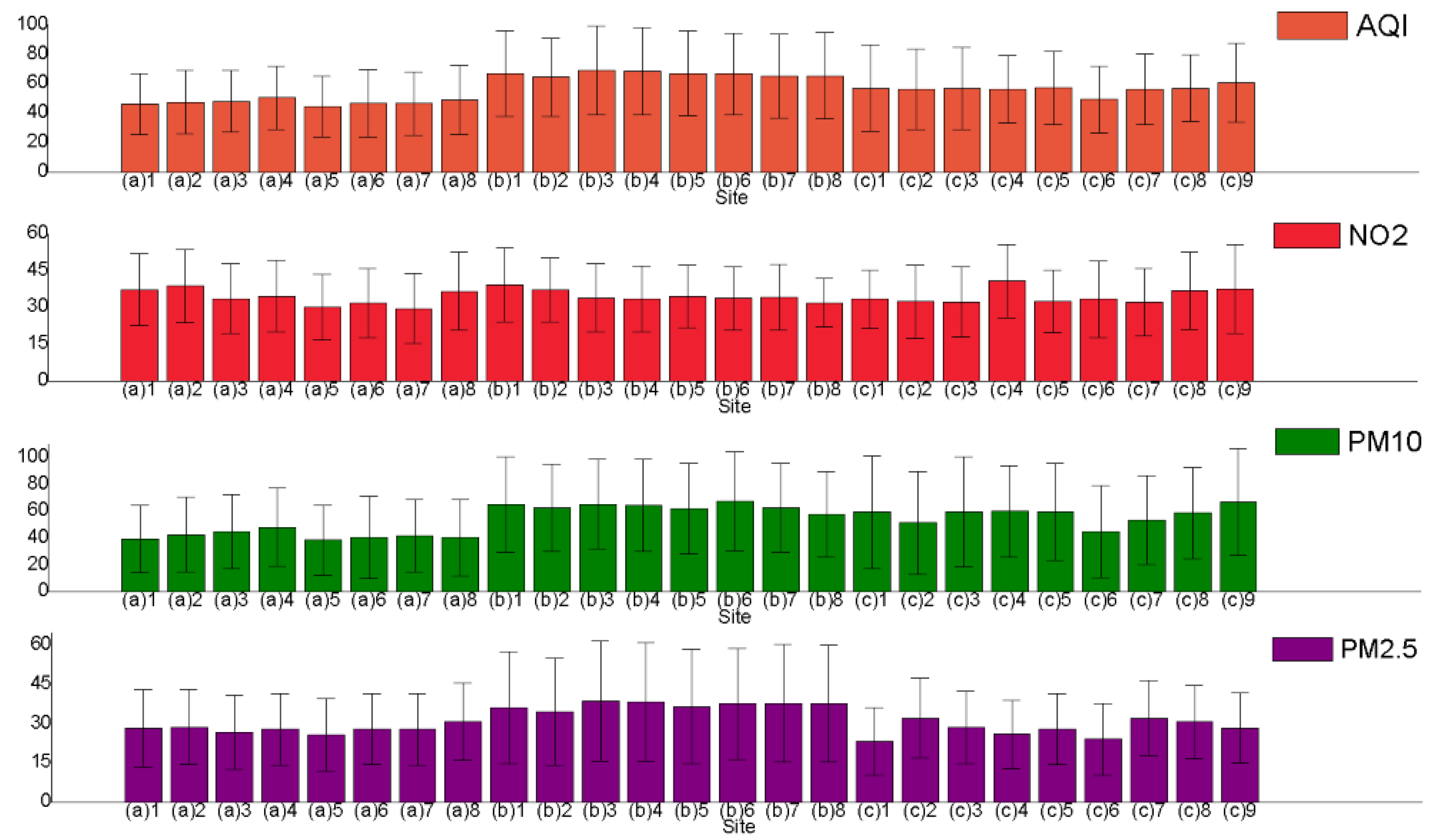
2.1. Air Pollution Data

As early as January 2013, the Ministry of Environmental Protection of China (MEPC) began to release real-time air pollution monitoring information over 74 major cities to the public [34]. In this study, the air pollution data used to determine urban air quality comes from 8 air quality-monitoring sites (Figure 1a) located in the central urban area of the Shanghai Outer Ring Road, 8 sites (Figure 1b) within the Fifth Ring Road of Beijing, and 9 sites (Figure 1c) in the main urban area of Nanjing. The location of these quality-monitoring sites is shown in Figure 1a–c. These sites are not distributed inside the street, but in open-air areas of residential areas and parks.

The hourly data for these 25 sites from May to October 2019 were collected, including AQI, NO₂, PM10 and PM2.5 (http://datacenter.mep.gov.cn/). The brief description of the MEPC’s measurement systems to measure the air pollutants is shown in

Table 1. The brief description of the measurement systems to measure the air pollution indexes.

Air Pollution Index	Unit	Measurement Method
NO2	μg/m3	Chemiluminescence method
PM10	μg/m3	Micro oscillating balance method and β-absorption method
PM2.5	μg/m3	Micro oscillating balance method and β-absorption method
AQI	non-dimensional	Calculated from six atmospheric pollutants [38]

[35,36,37]. Different from NO₂, PM10 and PM2.5, AQI is calculated from six atmospheric pollutants in this measurement systems [35].

Table 2. The values of NO₂, PM10, PM2.5 and AQI corresponding to different air quality levels.

Air Quality Level	AQI	NO2 (μg/m3)	PM10 (μg/m3)	PM2.5 (μg/m3)
I	0–50	0–40	0–50	0–35
II	51–100	41–80	51–150	36–75
III	101–150	81–180	151–250	76–115
IV	151–200	181–280	251–350	116–150
V	201–300	281–565	351–420	151–250
VI	>300	>565	>420	>250

lists the values of NO₂, PM10, PM2.5 and AQI corresponding to different air quality levels [38]. The higher the values, the worse the air quality. To minimize the impact of meteorological factors on air quality, the air pollution indexes (AQI, NO₂, PM10 and PM2.5) of different sites are the average of each indicator for each site, which were calculated separately by hourly data. To indicate how much pollution might vary across the summer season, the standard deviation (SD) for each parameter at each site were also calculated.

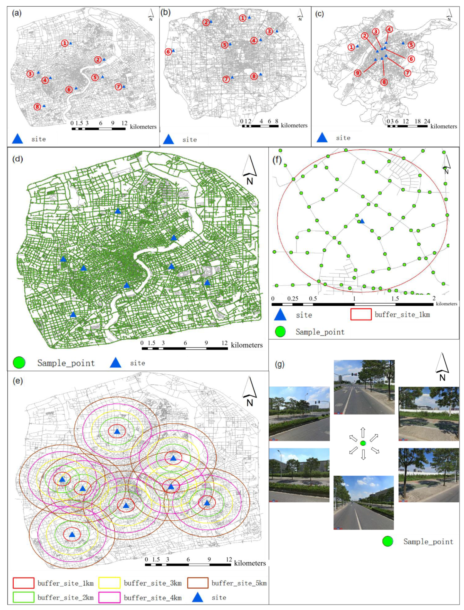
2.2. Street View Image Data

In this study, street view images were extracted from Baidu Map (https://map.baidu.com) in 2019, which is similar to Google Maps. From the street data of OpenStreetMap [39], we extracted road vector lines within the Fifth Ring Road of Beijing, the outer ring road of Shanghai, and the main urban area of Nanjing. Referring to relevant research [21,40] and considering efficiency and details, we set the sampling points at intervals of 100 m on the road vector line and compiled a script to crawl the street view images within a 50 m radius from the sampling point from Baidu map. Figure 1d shows the distribution of sampling points within the outer ring of Shanghai. As shown in Figure 1g, we obtained street view images in six directions at each sampling point, including azimuth angles of 0, 60, 120, 180, 240, and 300. The size of these images is 600 × 600 pixels, and the vertical angle is 0°. The meaning of selecting a vertical angle of 0° is to use the simplest standard to unify all images, avoiding a difference in standards when extracting information from different streets due to the different elevation angles of images, which makes images from different streets lose comparability. If we use a unified elevation angle for all images, as in the case of 0°, there will always be some street view images that cannot show the full extent (top or bottom) of the trees or buildings, we need to select different elevation angles for some streets to make the images always show the full extent of the trees or buildings appropriately, which will lead to different rules of the images obtained, and affect the comparability of the indexes obtained between different streets.

A total of 687,354 images were collected, of which 174,252 were in the fifth ring road of Beijing, 281,070 were in the main urban area of Nanjing, and 232,032 were in the central urban area of the outer ring of Shanghai. To analyze the effects of street greening and buildings in different ranges on urban summertime air quality, we extracted street view image data for different radii from air quality-monitoring sites in the study area, including 0–1, 1–2, 2–3, 3–4 and 4–5 km (Figure 1e). Figure 1f shows the detailed spatial distribution of sampling points within a certain radius of an air quality-monitoring site in Shanghai.

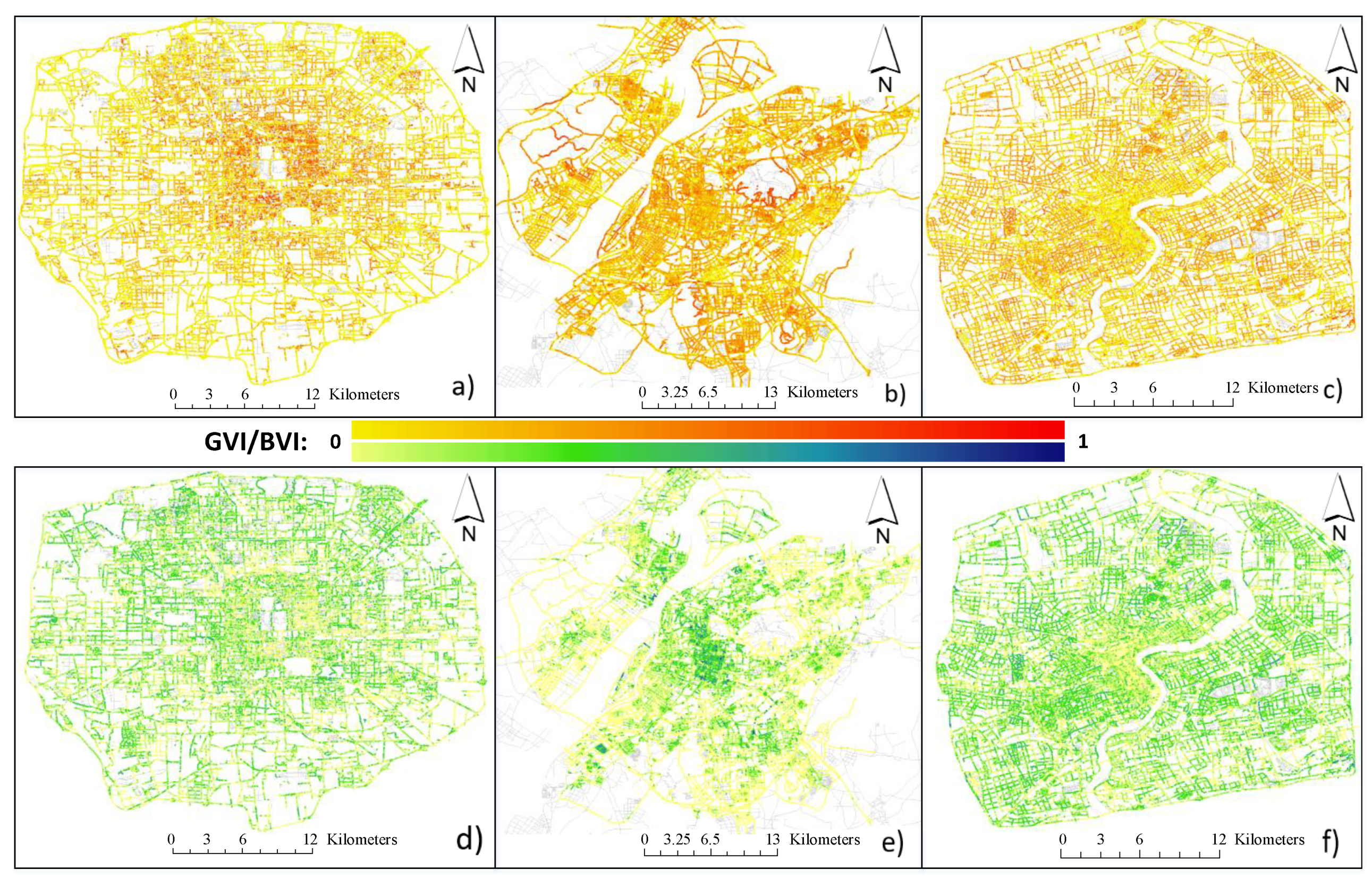
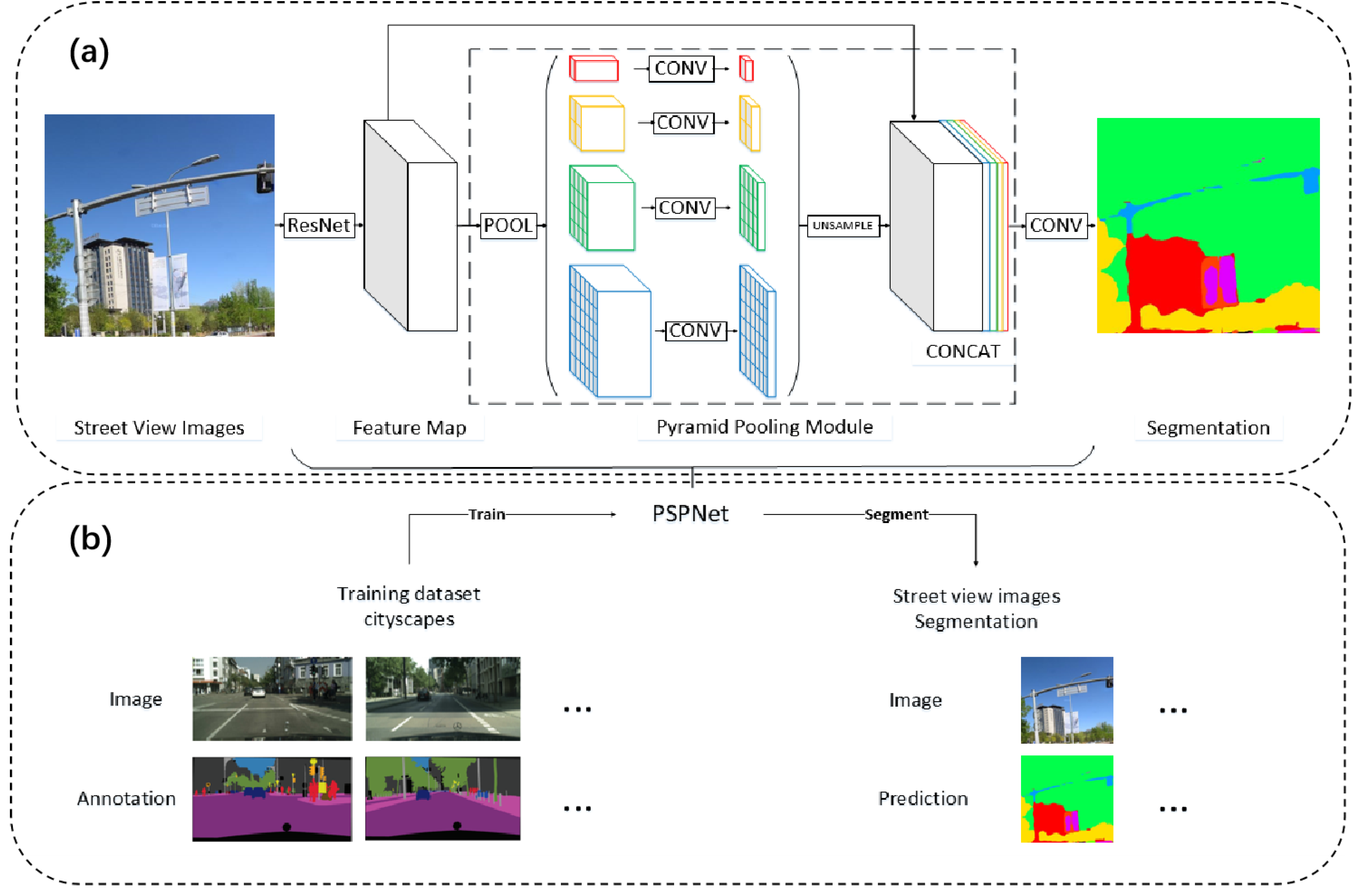
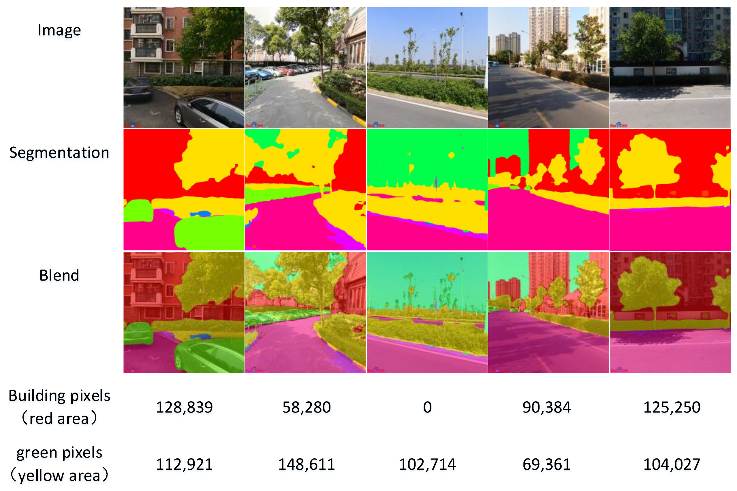
2.3. Street View Image Segmentation

A pyramid scene phrase network (PSPNet) [30] was used to segment street view images in this study. Most advanced semantic segmentation methods are based on a fully connected network (FCN). However, the convolutional neural network (CNN)’s empirical acceptance domain is much smaller than the theoretical acceptance domain, especially at the high level [41], and the FCN-based model lacks appropriate strategies to fully merge important global scene priors, resulting in the occurrence of most segmentation errors [30]. To solve this problem, PSPNet introduces a pyramid pooling module, which realizes context aggregation based on different regions, improves the ability to use global context information, and makes the final prediction more reliable.

Figure 2a shows the structure of the PSPNet. First, an image is input into a pre-training deep residual network [42] (ResNet) to extract the feature map of the image. Then, the feature map is input into the pyramid pooling module, and the output of different levels is obtained by using four levels of pyramids. The output of different-sized feature maps is sampled up, and the same-sized feature map is obtained by bilinear interpolation. Then, the features of different levels are aggregated into the pyramid global prior. This module is a hierarchical global prior, which reduces the loss of context information between different sub-regions by fusing the features of four different pyramid scales. Then, in the last part of the pyramid pooling module, the global prior of the pyramid is concatenated to the original feature map. Finally, the final prediction result of the input is generated through the convolution layer.

The flow to segment street view images is shown in Figure 2b. The collected street view image data are input into the trained PSPNet network, and the number of greening and building pixels in each street view image is output. The PSPNet model trained on the cityscape dataset [43] was used. Cityscape contains 5000 high-quality, pixel-level, fine-annotation street view images from 50 cities. In the annotation data, plant and buildings are marked pixel by pixel. The trained model can accurately identify the greening and building in the street view image. The pixel-wise accuracy for buildings is 93.2%, and that for plants is 93.4% [30].

2.4. Quantity of Street Greening and Street Buildings

The green view index (GVI) has been widely used in various urban green spaces [32], and many scholars have used GVI to quantify the greening in streetscapes and conduct many research studies [19,27,32,44,45,46]. There are some differences in the calculation formulas of GVI in different studies, with the main reason being the difference in data, including the difference in the number of street view images selected at each sampling point [19,27] and the difference in vertical angles [32,45].

In Section 2.2 and Section 2.3, images in six directions at each sampling point were obtained, and the numbers of pixels for greening and buildings were calculated. The azimuths of these images are 0°, 60°, 120°, 180°, 240°, and 300°, and the vertical angle is 0°. The field of view of the images is 60 degrees, so the six images from one sampling point cover the surrounding 360° scene and there is no overlap between the images. Therefore, when quantifying street greening based on street view data, the GVI formula used at each sampling point is as follows:

$$GVI\_sample=\frac{{\displaystyle \sum _{i=1}^{6}pixel{s}_{g\_i}}}{{\displaystyle \sum _{i=1}^{6}pixel{s}_{t\_i}}}$$

(1)

In Formula (1), $pixel{s}_{g\_i}$ represents the number of pixels of greening extracted from each image, and $pixel{s}_{t\_i}$ represents the total number of pixels per image. Based on Formula (1), Formula (2) was proposed to quantify street greening within a certain radius of air quality-monitoring sites, where n represents the number of sampling points within the range and $GVI\_sampl{e}_j$ is the GVI value calculated at each sampling point.

$$GVI\_site=\frac{{\displaystyle \sum _{j=1}^{n}GVI\_sampl{e}_j}}{n}$$

(2)

To quantify the street buildings, we proposed a quantitative indicator BVI (building view index), which is similar to the quantitative index GVI of street greening. The formulation includes Formula (3) to quantify street buildings at each sample point and Formula (4) to quantify street buildings within a certain radius of air quality-monitoring sites. $pixel{s}_{b\_i}$ represents the number of pixels of the buildings extracted from each image, and $BVI\_sampl{e}_j$ represents the BVI value calculated at each sampling point.

$$BVI\_sample=\frac{{\displaystyle \sum _{i=1}^{6}pixel{s}_{b\_i}}}{{\displaystyle \sum _{i=1}^{6}pixel{s}_{t\_i}}}$$

(3)

$$BVI\_site=\frac{{\displaystyle \sum _{j=1}^{n}BVI\_sampl{e}_j}}{n}$$

(4)

2.5. Covariates

The length of the streets within the different radii of the monitoring site was taken into consideration because it was considered to be related to summertime air pollution in the urban center area. The street length may reflect transport emissions and the amount of street dust within this area. The number of sampling points is used to quantify the total street length because we set a sampling point every 100 m along the street when collecting street view image data.

3. Statistical Analysis

We fitted multi-level regression models to explore the associations of street greening and street buildings with urban summertime air pollution, taking the air pollution indexes (NO₂, PM2.5, PM10, AQI) of each site as the outcome and controlling the street length variables.

To analyze the associations of the vertical distribution of street greening and street buildings with the air pollution indexes, four types of models (Models a1–a3, c1) were fitted. The first type of model (Models a1) is the baseline model and only contains street length variables within different radii of the air pollution-monitoring site. To test whether street greening and street building variables can improve the goodness-of-fit, the street greening variables (Models a3) and street buildings (Models a2) variables within different radii of the air pollution-monitoring site are added, respectively. The fourth type of model (Models c1) includes the variables of both street greening and street buildings.

To analyze the influence of streets within different radii of the air pollution-monitoring site on the air pollution indexes, five models (Models b1–b4, c1) were fitted. The baseline model (Model b1) includes street length variables, street greening variables, and street building variables within the range of 0–1 km of the air pollution-monitoring site. To test whether expanding the radius of the air pollution-monitoring site can improve the goodness-of-fit, the other four types of models added street-related variables within radii of 0–2, 0–3, 0–4, and 0–5 km of the air pollution-monitoring site (Models b2, 0–1 and 0–2 km; Models b3, 0–1, 1–2 and 2–3 km; Models b4, 0–1, 1–2, 2–3 and 3–4 km). Models c1 includes the variables of street length, street greening and street buildings within radii of 0–1, 1–2, 2–3, 3–4, and 4–5 km of the air pollution-monitoring site.

The Akaike information criterion (AIC) [46] and Bayesian information criterion (BIC) [47] were used to evaluate the performance of the model. Based on information theory [48], AIC and BIC are tow model selection criterions. The AIC and BIC scores are calculated as Formulas (5) and (6), where $\theta$ represents the model parameters, $L\widehat{(}\theta )$ is the likelihood of the candidate model given the data when evaluated at the maximum likelihood estimate of $\theta$ [49], $k$ represents the number of the model parameters, n represents the number of samples.

$$AIC=-2\log L\widehat{(}\theta )+2k$$

(5)

$$BIC=-2\log L\widehat{(}\theta )+k\log n$$

(6)

The AIC or BIC scores in isolation is meaningless [48], the “isolation” here means focus only on scores in a single model. By calculating the AIC and BIC scores of all candidate models, the “best” model is the candidate model with the lowest AIC or BIC scores among all candidate models. The smaller the AIC and BIC scores, the better the goodness-of-fit and performance. In addition, we reported the p-values and 95% confidence intervals for all models. p-values < 0.05 were considered statistically significant. Spss22.0 was used for statistics.

4. Results

4.1. Air Pollution and Street View Metrics

The average air pollutions, including AQI, NO₂, PM10, and PM2.5 at 25 sites from May to October 2019, were calculated, and the standard deviation (SD) was calculated for each parameter at each site (Figure 3). The Intersect Analysis method in ArcGIS 10.5 was used to calculate the number of sampling points (Total = 430,584) within different radius of each site as a street length variable. Detailed information on the air quality index and street length can be found in Tables S1 and S2 of the Supplementary Materials.

The greening and building areas in the street view images were accurately extracted by the trained PSPNet model. Figure 4 shows the segmentation results of some images. The yellow area is the greening area, and red is the buildings area. It can be found that there is sometimes a vertical building behind the vertical greenery in street view images. Previous studies have shown that the vertical structure closest to the street has an important influence on pollutant diffusion. The field monitoring results of Xilin North Road and Wencheng road in Shanghai [49] show that the pollutant diffusion in the street is obviously affected by the vertical structure close to the street (such as the green plants). The green plants between the street and the street buildings significantly reduce the diffusion of pollutants from the green plants near the street to the buildings. Therefore, when we extract the vertical structure from the street view image, we extract the vertical structure closest to the street, and ignore the vertical buildings covered by vertical greenery. Figure 5 plots the spatial distribution of GVI_sample and BVI_sample in the study area. It can be found that there are differences in the spatial distribution. GVI_sample (Mean = 0.2103, SD = 0.1314) and BVI_sample (Mean = 0.1955, SD = 0.1436) of sampling points in different radius ranges of each air quality-monitoring site were calculated. The street greening index GVI_site (Mean = 0.2165, SD = 0.0412) and street building index BVI_site (Mean = 0.1854, SD = 0.0658) within different radii at each site were calculated. The descriptive statistical results of different radii of all air pollution-monitoring sites in all cities are shown in

Table 3. Descriptive statistics of BVI_site and GVI_site.

Index	Buffer_Distance (km)	Mean (SD)	Min	Max
BVI_site	0–1	0.1813 (0.0767)	0.0581	0.3117
	1–2	0.1882 (0.0688)	0.0658	0.3120
	2–3	0.1898 (0.0570)	0.0777	0.2780
	3–4	0.1840 (0.0691)	0.0542	0.2558
	4–5	0.1816 (0.0643)	0.0524	0.2676
GVI_site	0–1	0.2231 (0.0552)	0.1269	0.3130
	1–2	0.2149 (0.0385)	0.1464	0.3330
	2–3	0.2061 (0.0287)	0.1494	0.2548
	3–4	0.2117 (0.0256)	0.1508	0.2564
	4–5	0.2045 (0.0235)	0.1548	0.2545

, which reflects the overall situation of BVI_site and GVI_site in the studied area and the difference of BVI_site and GVI_site among different sites. For detailed results of GVI_site and BVI_site, see Table S3 of the Supplementary Materials.

4.2. Multilevel Regression Model

From the models considering all variables (Model c1), we observed the associations of street greening and street buildings with the air pollution indexes within different radii of the air quality-monitoring site. Within the radius of 1 km, there is a positive association (p = 0.077) between street buildings and NO₂. Within the radius of 1–2 km, street greening (p = 0.042) has a significant negative association with NO₂, and street length has a positive association with AQI (p = 0.072) and PM10 (p = 0.062). Within the 3–4-km radius of the air quality-monitoring site, there is a negative association between street greening and PM2.5 (p = 0.065), and there is a significant negative association between street greening and AQI (p = 0.034), PM10 (p = 0.028). However, within the radius of 4–5 km, there is no significant association between street vegetation, street buildings, street length and the air quality index of air monitoring sites.

Table 4. AIC and BIC scores of the models.

		Model a1	Model a2	Model a3	Model b1	Model b2	Model b3	Model b4	Model c1
AQI	AIC	3933	3758	3664	4379	4332	4039	3607	3348
	BIC	3940	3771	3678	4384	4341	4051	3622	3369
PM10	AIC	4125	4052	3958	4690	4614	4370	3935	3647
	BIC	4133	4066	3971	4695	4622	4383	3951	3666
PM2.5	AIC	3650	3406	3203	3785	3660	3399	3170	3011
	BIC	3657	3419	3217	3790	3668	3411	3186	3031
NO2	AIC	3021	2740	2837	3076	2755	2477	2471	2362
	BIC	3028	2753	2850	3081	2764	2489	2487	2382

(Models a1–a3, c1) shows the influence of street buildings and street greening variables on summertime air pollution for all air pollution indices, including AQI, NO₂, PM10, and PM2.5. Adding street greening variables (Model a3) or street building variables (Model a2) to the street length variables (Model a1) leads to a decrease in the AIC scores and BIC scores, which means the model’s goodness-of-fit and performance are improved. Models c1, which includes street greening, street building and street length variables, received the lowest AIC and BIC scores, indicating the highest goodness-of-fit and the best performance.

The results of the models (Table 4, Models b1–b4, Models c1) revealed the influence of street length, street greening, and street building variables on summertime air pollution within different radii of the air pollution-monitoring site for the models with different air pollution indexes as the outcome, including AQI, NO₂, PM10, and PM2.5. As the radius of the air pollution-monitoring site increases (from 0–1 to 0–5 km, Models b1–b4, Models c1), that is, considering the street length variables, street greening and street building variables within a larger radius of the air pollution-monitoring site (from 0–1 to 0–5 km), the model’s AIC scores and BIC scores decrease, indicating the increase of the model’s goodness-of-fit and performance. Among them, Models c1, which includes the variables of street length, street greening and street buildings with radii of 0–5 km (0–1, 1–2, 2–3, 3–4, and 4–5 km) of the air pollution-monitoring site, has the lowest AIC and BIC scores, indicating that streets within 0–5 km affect the air pollution indexes of the air quality-monitoring sites.

However, although the model improves (lower AIC and BIC) as more variables and greater distances from the monitoring sites are included, the best outcome occurs when variables within all different radii of the site are included (Models c1; 0–1, 1–2, 2–3, 3–4 and 4–5 km); however, are the influence of the street variables with different radii of the site (0–1, 1–2, 2–3, 3–4, and 4–5 km) on the air pollution indexes different? For the models with NO₂, PM10, and PM2.5 as the outcome, we find that, with the increase of the distance between the new street variables and the site (

Table 5. ∆R2.

	Model b1	Model b2	Model b3	Model b4	Model c1
NO2	0.209	0.322	0.171	0.005	0.049
PM2.5	0.156	0.16	0.237	0.14	0.071
PM10	0.152	0.105	0.245	0.253	0.093

; e.g., Models b2 added variables with a radius of 1–2 km of the site compared with Models b1 and Models c1 added variables with a radius of 4–5 km compared with Models b4), the R-square change of the different air pollution indexes mostly becomes smaller. The R-square changes for the 3–4- and 4–5-km radii are almost the smallest in the models (Table 5, NO₂, PM2.5). The smaller the change of R-square is, the lower the ability of the new variable is to interpret the result. This shows that, although the street variables within 3–4 or 4–5 km still have influence on the model (Table 4, Models b4, Models c1), the influence is reduced compared with the street variables within radius of 0–1, 1–2 or 2–3 km (Table 5, Models b1–c1). When the radius of the air pollution-monitoring site is large (from 0–1 to 4–5 km), the influence of the street on the air pollution indexes is reduced.

5. Discussion

This study analyzes the associations of the distribution and vertical structure of urban street greening and street buildings with summertime air pollution in the urban center area at city scale for the first time, using street view image data and a deep-learning algorithm. Most of the previous research studied the association between urban green space and air quality based on small-scale streets [14,15] or large-scale horizontal distribution of urban green space [17,18].

5.1. The Associations between Streets and Summertime Air Pollution

Our results show that there is a significant association between summertime air pollution and urban streets. The vertical distributions of urban street greening and street buildings have an influence on air pollution, and the increase of the vertical distribution of street greening has a significant positive role in preventing the diffusion of street pollution, while the increase of street length within a certain radius aggravates air pollution in urban areas.

It has been proved that the vertical structure of green space [14] and buildings [50] for specific streets at small scale, as well as the large-scale urban block green space distribution [17], has an effect on air pollution diffusion. However, in view of the effect of the vertical distribution of greening and buildings on air pollution in a large range of urban streets, there is still a lack of understanding. As the street view image data reflect the vertical structure of the street greening and buildings, by using the street view image data, we found that the increase of the vertical distribution of street greening can effectively reduce the summertime air pollution from the streets. The increase of the vertical distribution of street greening often means the increase of diversity of plant types, and the difference in vertical distribution of green space has an influence on the filtering effect [14], such as lower shrubs and higher trees. This just explains the significant negative association between the street greening and air quality index in this study.

In view of the influence of street buildings on the diffusion of summertime air pollution, previous studies [50] have shown that the vertical distribution of buildings in streets will have an impact on the light, airflow, etc., in the streets, thus affecting the diffusion of pollutants. We found that the vertical distribution of street buildings within 1 km was positively associated with the NO₂ index of air pollution (p = 0.077), and the model with the street buildings variables added (Model a2) has lower AIC and BIC scores than the models that only have street length variables (Model a1). The vertical distribution of street buildings may have an impact on the airflow in the street, thus affecting the diffusion of air pollution in the street, and finally affecting the urban summertime air pollution in this area.

The association between the summertime air pollution in the central area of the city and the street length in the area was found. Research shows that [1,51] a large part of the source of urban summertime air pollution comes from street dust, automobile exhausts, etc. Our research results support this view. The increase of street length, to some extent, represents the increase of transport emissions and street dust. We found that there was a positive association (p < 0.1) between the street length and the air quality pollution index within the radius of 1–2 km. With the increase of the length of streets in this area, summertime air pollution becomes worse.

Streets within a certain radius have an impact on the summertime air pollution in the center of the region, but the impact of streets within different radius ranges on the air pollution indexes is different. Our results show that, within the range of 4–5 km, there are no significant associations (p > 0.1) of street greening, street buildings and street length with the summertime air pollution indexes of air monitoring sites. This indicates that the farther the distance is, the smaller the impact is on the summertime air pollution. Research [17] shows that the massive green space of the city will have an impact on the air quality. Therefore, we thought it likely that the air pollution from the streets far away will be absorbed and blocked by the urban green space between the streets such that the impact on the index of air pollution-monitoring sites is weakened.

5.2. Strengths and Limitations

There are numerous strengths of our research. First, we focus on the impact of the vertical distribution of street green space on air pollution at a large scale, compared with the major studies focusing on the diffusion of pollution in streets on a small scale [7,11]. Secondly, it is innovative, efficient and reliable to use street view image data to analyze the effect of street greening and street buildings on summertime air pollution diffusion, rather than through the field measurement [14] or simulation [7] of each street. Street view images capture the vertical distribution of street greening and buildings. Thirdly, a machine-learning method is used to realize the automatic extraction of information of large-scale street view data, and our deep-learning method enables us to extract greening and building area more effectively and accurately compared with pixel-wise classification [52] and traditional methods.

However, there are many limitations in our research. First of all, the street view image data of Baidu map is taken at a specific time, so the street greening and buildings obtained are the values of a certain time rather than the average value. However, the indicators of street greening and building are still reliable because the change of green space and buildings is slow [7]. Secondly, although the air pollution data adopts the average data from May to October to eliminate the impact of meteorological factors as much as possible, the meteorological factors may still have some impact on the results, and the impact on the results is not clear at present. Finally, although we have obtained a large amount of street view image data, compared with all cities in China, the data volume is still small, so the applicability of the research results to other cities in China remains to be discussed.

Therefore, we will carry out further study in the future work. As we have mentioned, there are some shortcomings in this paper. First of all, in the future work, maybe we could consider all major cities in China to study the applicability of the research results in China. Secondly, the current work was limited to a few cities in China, and in future work we can use Google data to expand the study to more countries around the world. It should be interesting to compare the results among different countries. Finally, maybe we can train a more powerful neural network to extract more detailed vegetation types, such as grassland, trees, shrubs, etc., and the impact of different vegetation types on pollution can be analyzed more accurately.

6. Conclusions

This study shows that the vertical distribution of street buildings and street greening is related to the summertime air pollution in the central area of the city. The increase of the vertical distribution of street greening can prevent the diffusion of air pollution from the streets, which is in the central areas of Beijing, Nanjing and Shanghai in China. Compared with the existing field observation or numerical simulation, we use street view data and deep-learning methods to extract the vertical structure of greening and building areas. Our multilevel regions show that the vertical distribution of street greening within a certain radius around the monitoring site is significantly positively associated with the summertime air quality of the site, and the street length is negatively correlated with the air quality. With the increase of the distance from the street, the influence of the pollution from the street on the summertime air quality decreases. The main contribution of this paper is to use street view data sources and deep learning methods, to study the problem from another perspective. A feasible route by using street view data and deep learning method was established for further analysis. This paper has the following contributions:

• A method for measuring the vertical structure of street green space and street buildings in assessing summertime air pollution over a large scale of urban central areas is proposed.
• Use of deep-learning methods to extract the vertical distribution of street greening and buildings from street view images.
• The street green index and building index are proposed to quantify the street greening and street buildings within a certain radius.
• The association between the vertical structure of street green space and the summertime air pollution in the central area of the city on the urban scale is analyzed.

Our findings highlight the importance of measurement methods for the vertical structure of street green space and street buildings in assessing summertime air pollution over large-scale urban central areas. Combined with street view data and deep learning, it provides an efficient tool for street environment assessment, which is suitable for urban air pollution research. Our discovery of the relationship between the vertical structure of street green space and the summertime air pollution in the central area of the city can provide support for urban street planning. In the street planning of the urban center area, we should consider the different configurations of street green plants and street buildings and make a reasonable vertical distribution configuration so as to reduce the air pollution in the urban center area in the summer. The current work was limited to a few cities in China and, in future work, we can use Google data to expand the study to more countries around the world.

References

1. Liu, Z.; Hu, B.; Liu, Q.; Sun, Y.; Wang, Y.S. Source apportionment of urban fine particle number concentration during summertime in Beijing. Atmos. Environ. 2014, 96, 359–369. [Google Scholar] [CrossRef]
2. Abhijith, K.V.; Kumar, P.; Gallagher, J. Air pollution abatement performances of green infrastructure in open road and built-up street canyon environments—A review. Atmos. Environ. 2017, 162, 71–86. [Google Scholar] [CrossRef]
3. Jayasooriya, V.; Ng, A.; Muthukumaran, S.; Perera, B. Green infrastructure practices for improvement of urban air quality. Urban For. Urban Green. 2017, 21, 34–47. [Google Scholar] [CrossRef]
4. Liu, J.; Cao, Z.; Zou, S.; Liu, H.; Hai, X.; Wang, S.; Duan, J.; Xi, B.; Yan, G.; Zhang, S.; et al. An investigation of the leaf retention capacity, efficiency and mechanism for atmospheric particulate matter of five greening tree species in Beijing, China. Sci. Total Environ. 2018, 616, 417–426. [Google Scholar] [CrossRef]
5. Pugh, T.A.M.; MacKenzie, A.R.; Whyatt, J.D.; Hewitt, C.N. Effectiveness of Green Infrastructure for Improvement of Air Quality in Urban Street Canyons. Environ. Sci. Technol. 2012, 46, 7692–7699. [Google Scholar] [CrossRef] [Green Version]
6. Weber, F.; Kowarik, I.; Säumel, I. Herbaceous plants as filters: Immobilization of particulates along urban street corridors. Environ. Pollut. 2014, 186, 234–240. [Google Scholar] [CrossRef]
7. Vardoulakis, S.; Valiantis, M.; Milner, J. Operational air pollution modelling in the UK—Street canyon applications and challenges. Atmos. Environ. 2007, 41, 4622–4637. [Google Scholar] [CrossRef]
8. Nowak, D.J.; Hirabayashi, S.; Bodine, A.; Hoehn, R. Modeled PM2.5 removal by trees in ten U.S. cities and associated health effects. Environ. Pollut. 2013, 178, 395–402. [Google Scholar] [CrossRef]
9. Zhang, H.; Wang, Y.; Li, S. Study on the Influence of the Street Side Buildings on the Pollutant Dispersion in the Street Canyon. Procedia Eng. 2015, 121, 37–44. [Google Scholar] [CrossRef]
10. Salmond, J.A.; Williams, D.E.; Laing, G. The influence of vegetation on the horizontal and vertical distribution of pollutants in a street canyon. Sci. Total Environ. 2013, 443, 287–298. [Google Scholar] [CrossRef]
11. Morakinyo, T.E.; Lam, Y.F.; Hao, S. Evaluating the role of green infrastructures on near-road pollutant dispersion and removal: Modelling and measurement. J. Environ. Manag. 2016, 182, 595–605. [Google Scholar] [CrossRef] [PubMed]
12. Jeanjean, A.; Monks, P.S.; Leigh, R.J. Modelling the effectiveness of urban trees and grass on PM2.5 reduction via dispersion and deposition at a city scale. Atmos. Environ. 2016, 147, 1–10. [Google Scholar] [CrossRef] [Green Version]
13. Iachou, K.; Livada, I.; Santamouris, M. Experimental study of temperature and airflow distribution inside an urban street canyon during hot summer weather conditions: Part 1: Air and surface temperatures. Build. Environ. 2008, 13, 1383–1392. [Google Scholar]
14. Brantley, H.L.; Hagler, G.S.; Deshmukh, P.J.; Baldauf, R. Field assessment of the effects of roadside vegetation on near-road black carbon and particulate matter. Sci. Total Environ. 2014, 469, 120–129. [Google Scholar] [CrossRef] [Green Version]
15. Deshmukh, P.; Isakov, V.; Venkatram, A.; Yang, B.; Zhang, K.M.; Logan, R.; Baldauf, R. The effects of roadside vegetation characteristics on local, near-road air quality. Air Qual. Atmos. Health 2018, 12, 259–270. [Google Scholar] [CrossRef] [Green Version]
16. Tong, Z.; Whitlow, T.H.; Macrae, P.F.; Landers, A.J.; Harada, Y. Quantifying the effect of vegetation on near-road air quality using brief campaigns. Environ. Pollut. 2015, 201, 141–149. [Google Scholar] [CrossRef]
17. Chen, L.; Liu, C.; Zou, R. Experimental examination of effectiveness of vegetation as bio-filter of particulate matters in the urban environment. Environ. Pollut. 2016, 208, 198–208. [Google Scholar] [CrossRef]
18. Li, J.K. Modeling and Analysis of Influence of Road Green Belt Spatial Structure Design on Pollutant Diffusion. Environ. Sci. Manag. 2018, 43, 75–78. [Google Scholar]
19. Zhang, Y.; Dong, R. Impacts of Street-Visible Greenery on Housing Prices: Evidence from a Hedonic Price Model and a Massive Street View Image Dataset in Beijing. ISPRS Int. J. Geo. Inf. 2018, 7, 104. [Google Scholar] [CrossRef] [Green Version]
20. Lu, Y.; Sarkar, C.; Xiao, Y. The effect of street-level greenery on walking behavior: Evidence from Hong Kong. Soc. Sci. Med. 2018, 208, 41–49. [Google Scholar] [CrossRef]
21. Helbich, M.; Yao, Y.; Liu, Y.; Zhang, J.; Liu, P.; Wang, R. Using deep learning to examine street view green and blue spaces and their associations with geriatric depression in Beijing, China. Environ. Int. 2019, 126, 107–117. [Google Scholar] [CrossRef] [PubMed]
22. He, L.; Paez, A.; Liu, D. Built environment and violent crime: An environmental audit approach using Google Street View. Comput. Environ. Urban Syst. 2017, 66, 83–95. [Google Scholar] [CrossRef]
23. Fan, Z.; Bolei, Z.; Liu, L. Measuring human perceptions of a large-scale urban region using machine learning. Landsc. Urban Plan. 2018, 180, 148–160. [Google Scholar]
24. Zeng, L.; Lu, J.; Li, W. A fast approach for large-scale Sky View Factor estimation using street view images. Build. Environ. 2018, 135, 74–84. [Google Scholar] [CrossRef]
25. Gonga, F.Y.; Zeng, Z.C.; Zhang, F. Mapping sky, tree, and building view factors of street canyons in a high-density urban environment. Build. Environ. 2018, 134, 155–167. [Google Scholar] [CrossRef]
26. Middel, A.; Lukasczyk, J.; Zakrzewski, S. Urban form and composition of street canyons: A human-centric big data and deep learning approach. Landsc. Urban Plan. 2019, 183, 122–132. [Google Scholar] [CrossRef]
27. Liang, C.; Sensen, C.; Wenwen, Z. Use of Tencent Street View Imagery for Visual Perception of Streets. ISPRS Internatl. J. Geo. Inf. 2017, 6, 265. [Google Scholar]
28. Long, J.; Shelhamer, E.; Darrell, T. Fully Convolutional Networks for Semantic Segmentation. IEEE Trans. Pattern Anal. Mach. Intell. 2014, 39, 640–651. [Google Scholar]
29. Badrinarayanan, V.; Kendall, A.; Cipolla, R. SegNet: A Deep Convolutional Encoder-Decoder Architecture for Scene Segmentation. IEEE Trans. Pattern Anal. Mach. Intell. 2017, 39, 2481–2495. [Google Scholar] [CrossRef]
30. Zhao, H.; Shi, J.; Qi, X.; Wang, X.; Jia, J. Pyramid Scene Parsing Network. In Proceedings of the IEEE Conference on Computer Vision and Pattern Recognition, Honolulu, HI, USA, 21–26 July 2017. [Google Scholar]
31. Rossetti, T.; Lobel, H.; Rocco, V.; Hurtubia, R. Explaining subjective perceptions of public spaces as a function of the built environment: A massive data approach. Landsc. Urban Plan. 2019, 181, 169–178. [Google Scholar] [CrossRef]
32. Dong, R.; Zhang, Y.; Zhao, J. How Green Are the Streets Within the Sixth Ring Road of Beijing? An Analysis Based on Tencent Street View Pictures and the Green View Index. Int. J. Environ. Res. Public Health 2018, 15, 1367. [Google Scholar] [CrossRef] [PubMed] [Green Version]
33. Lu, Y.; Lu, J.; Zhang, S.; Hall, P. Traffic signal detection and classification in street views using an attention model. Comput. Vis. Media 2018, 4, 253–266. [Google Scholar] [CrossRef] [Green Version]
34. Fan, H.; Zhao, C.; Yang, Y. A comprehensive analysis of the spatio-temporal variation of urban air pollution in China during 2014–2018. Atmos. Environ. 2020, 220, 117066. [Google Scholar] [CrossRef]
35. Song, Z.; Deng, Q.; Ren, Z. Correlation and principal component regression analysis for studying air quality and meteorological elements in Wuhan, China. Environ. Prog. Sustain. Energy 2019, 39. [Google Scholar] [CrossRef]
36. Ministry of Ecology and Environment of the People’s Republic of China. Determination of Atmospheric Articles PM10 and PM2.5 in Ambient Air by Gravimetric Method (HJ 618–2011). Available online: http://www.mee.gov.cn/ywgz/fgbz/bz/bzwb/jcffbz/201109/W020120130460791166784.pdf (accessed on 10 January 2020).
37. Ministry of Ecology and Environment of the People’s Republic of China. Specifications and Test Procedures for Ambient Air Quality Continuous Automated Monitoring System for SO2, NO2, O3 and CO (HJ 654-2013). Available online: http://www.cnemc.cn/jcgf/dqhj/201711/P020181010540087558130.pdf (accessed on 10 January 2020).
38. Ministry of Ecology and Environment of the People’s Republic of China. Technical Regulation on Ambient Air Quality Index (on Trial) (HJ 633–2012). Available online: http://www.mee.gov.cn/ywgz/fgbz/bz/bzwb/jcffbz/201203/W020120410332725219541.pdf (accessed on 10 January 2020).
39. Arsanjani, J.J.; Mooney, P.; Zipf, A. OpenStreetMap in GIScience: Experiences, Research, Applications; Springer: Cham, Switzerland, 2015. [Google Scholar]
40. Lu, Y. The Association of Urban Greenness and Walking Behavior: Using Google Street View and Deep Learning Techniques to Estimate Residents’ Exposure to Urban Greenness. Int. J. Environ. Res. Public Health 2018, 15, 1576. [Google Scholar] [CrossRef] [Green Version]
41. Zhou, B.; Khosla, A.; Lapedriza, A. Object Detectors Emerge in Deep Scene CNNs. arXiv 2014, arXiv:1412.6856. [Google Scholar]
42. He, K.; Zhang, X.; Ren, S.; Sun, J. Deep Residual Learning for Image Recognition. In Proceedings of the 2016 IEEE Conference on Computer Vision and Pattern Recognition (CVPR), Las Vegas, NV, USA, 27–30 June 2016; pp. 770–778. [Google Scholar]
43. Cordts, M.; Omran, M.; Ramos, S.; Rehfeld, T.; Enzweiler, M.; Benenson, R.; Franke, U.; Roth, S.; Schiele, B. The Cityscapes Dataset for Semantic Urban Scene Understanding. In Proceedings of the 2016 IEEE Conference on Computer Vision and Pattern Recognition (CVPR), Las Vegas, NV, USA, 27–30 June 2016; pp. 3213–3223. [Google Scholar]
44. Yang, J.; Zhao, L.; McBride, J.; Gong, P. Can you see green? Assessing the visibility of urban forests in cities. Landsc. Urban Plan. 2009, 91, 97–104. [Google Scholar] [CrossRef]
45. Li, X.; Zhang, C.; Li, W.; Ricard, R.; Meng, Q.; Zhang, W. Assessing street-level urban greenery using Google Street View and a modified green view index. Urban For. Urban Green. 2015, 14, 675–685. [Google Scholar] [CrossRef]
46. Akaike, H. A new look at the statistical model identification. IEEE Transact. Autom. Control 1974, 19, 716–723. [Google Scholar] [CrossRef]
47. Schwartz, G. Estimating the dimension of a model. Ann. Stat. 1978, 6, 31–38. [Google Scholar] [CrossRef]
48. Fabozzi, F.J.; Focardi, S.M.; Rachev, S.T. The Basics of Financial Econometrics (Tools, Concepts, and Asset Management Applications) In Appendix E: Model Selection Criterion: AIC and BIC [M]; John Wiley & Sons Inc.: Hoboken, NJ, USA, 2014. [Google Scholar]
49. Wang, Y.; Kang, Y.; Chen, Y. Influence of Buildings and Tree Planting on Air Pollutants Diffusion in Street Canyon. J. Donghua Univ. Nat. Sci. 2012, 38, 740–744. [Google Scholar]
50. Zhu, Q.; Kang, Y.; Yang, F. Impacts of upstream buildings on the flow fields and pollutant distributions in street canyons. China Environ. Sci. 2015, 35, 45–54. [Google Scholar]
51. Fu, L.; Hao, J.; He, D. The Emission Characteristics of Pollutants from Motor Vehicles in Beijing. Chin. J. Environ. Sci. 2000, 21, 68–70. [Google Scholar]
52. Larkin, A.; Hystad, P. Evaluating street view exposure measures of visible greenspace for health research. J. Expo. Sci. Environ. Epidemiol. 2018, 1, 447–456. [Google Scholar]
Figure 1. The study area’s distribution of air quality-monitoring sites and street view image data. (a) Road network and distribution of air quality-monitoring sites within the outer ring road of Shanghai. (b) Road and distribution of sites within the Fifth Ring Road in Beijing. (c) Road and distribution of sites within the main urban area of Nanjing. (d) Distribution of sampling points along the street within the outer ring of Shanghai. (e) For each site, the considered radius was ranged from 1 to 5 km with a 1-km interval. (f) Spatial distribution of sampling points around a site. (g) At each sampling point, the street view images with six azimuth angles (0, 60, 120, 180, 240, and 300) were collected. The vertical angle is 0 degrees, and the resolution is 600 × 600 pixels.
Ijgi 09 00500 g001
Figure 2. The architecture of PSPNet [30] (a) and the flow of street view image segmentation (b).
Ijgi 09 00500 g002
Figure 3. Mean and standard deviation (SD) for each parameter at each site.
Ijgi 09 00500 g003
Figure 4. The results of street view image segmentation.
Ijgi 09 00500 g004
Figure 5. Spatial distribution of GVI_sample and BVI_sample (values between 0~1). (a) Beijing, BVI; (b) Nanjing, BVI; (c) Shanghai, BVI; (d) Beijing, GVI; (e) Nanjing, GVI; (f) Shanghai, GVI.
Ijgi 09 00500 g005