Article

Semantic Integration of Raster Data for Earth Observation: An RDF Dataset of Territorial Unit Versions with their Land Cover

IRIT, Université de Toulouse, CNRS, 31062 Toulouse CEDEX 9, France
*
Author to whom correspondence should be addressed.
ISPRS Int. J. Geo-Inf. 2020, 9(9), 503; https://0-doi-org.brum.beds.ac.uk/10.3390/ijgi9090503
Submission received: 19 June 2020 / Revised: 4 August 2020 / Accepted: 19 August 2020 / Published: 21 August 2020
(This article belongs to the Special Issue Geographic Information Extraction and Retrieval)

Abstract

:
Semantic technologies are at the core of Earth Observation (EO) data integration, by providing an infrastructure based on RDF representation and ontologies. Because many EO data come in raster files, this paper addresses the integration of data calculated from rasters as a way of qualifying geographic units through their spatio-temporal features. We propose (i) a modular ontology that contributes to the semantic and homogeneous description of spatio-temporal data to qualify predefined areas; (ii) a Semantic Extraction, Transformation, and Load (ETL) process, allowing us to extract data from rasters and to link them to the corresponding spatio-temporal units and features; and (iii) a resulting dataset that is published as an RDF triplestore, exposed through a SPARQL endpoint, and exploited by a semantic interface. We illustrate the integration process with raster files providing the land cover of a specific French winery geographic area, its administrative units, and their land registers over different periods. The results have been evaluated with regards to three use-cases exploiting these EO data: integration of time series observations; EO process guidance; and data cross-comparison.

1. Introduction

Earth Observation (EO) is a domain that has greatly evolved in the previous years thanks to large-scale Earth monitoring programs, such as the US Landsat Program (https://www.usgs.gov/land-resources/nli/landsat) and the EU Copernicus Program (http://www.copernicus.eu/en). In particular, with the Copernicus program launched by the European Space Agency (ESA), data are collected by satellites and combined with observation data from sensor networks on the Earth’s surface. Nowadays, two types of Sentinel satellites are in production, several others being expected by 2030. Since 2015, Sentinel-1 and Sentinel-2 deliver high-quality Earth images (estimated between 8 TB to 10 TB of data daily), providing users with free, reliable, and up-to-date Earth image data and metadata. The availability of these data sources opened opportunities to better support existing domain-oriented applications and to boost emerging new ones, from agriculture to forestry, environmental monitoring to urban planning, climate studies, and disaster monitoring. These sources of data, coupled with the development of machine learning algorithms have boosted the image processing field and their application in the different domains.
One common way of representing the results of image processing algorithms is raster. A raster represents a rectangular grid of pixels and is produced from a predefined codification or classification dedicated to a specific analysis or need (e.g., a land cover classification). In this setting, each pixel contains a value to characterize the corresponding area (e.g., its representative land cover). Such representations may be automatically built by different algorithms, including machine learning. Many rasters can be provided for the same geographic area (e.g., a Sentinel-2 tile): they can be compared, combined, or used to generate a new one [1]. However, rasters are not human-readable. The interpretation of their content, either by users of decision support software tools, requires higher-level descriptions, based on the representation of spatial and temporal features.
In the EO field, one fundamental type of data is the Earth’s surface coverage or land cover (e.g., water, croplands, or urban). In many cases, land cover information is provided as a raster linked to a text file containing the naming convention of the land cover classes. Each pixel in the raster file is associated with one of these classes. These rasters may come in different formats. They are produced by different services as a result of massive time-series image processing under different resolutions [2]. Examples of land cover classifications are the Global Land Cover Share (GLC-SHARE), the European Corine Land Cover (CLC), and the French CESBIO Land Cover (CESBIO-LC). A further step to make use of land cover is to compute the percentage of each type of land cover on a given area (i.e., agricultural parcel), to identify the main land cover in this area. Land cover data can then be useful for the study of crop evolution, the progress of urban areas, or the impact of natural hazards. Moreover, the semantic representation of land cover data has been exploited for image annotation improving semantic search [3,4].
This paper addresses the integration of data calculated from rasters as a way of qualifying geographic units, based on their spatio-temporal features. We are interested in studying (i) the kind of ontology required to support knowledge extraction from EO data, to be able to describe homogeneously different analysis results (observed properties or indicators) described by the rasters; (ii) how to make accessible and usable rich EO data captured thanks to image processing and other kinds of related EO data; and (iii) how to keep track of the provenance of any produced data (data sources, raster calculation, semantic process). The contributions exposed in this paper address each of these challenges.
  • As a first contribution, we propose a generic vocabulary that allows the semantic and homogeneous description of spatio-temporal data to qualify predefined areas together with their provenance. This model is extendable to deal with any kind of observed EO property.
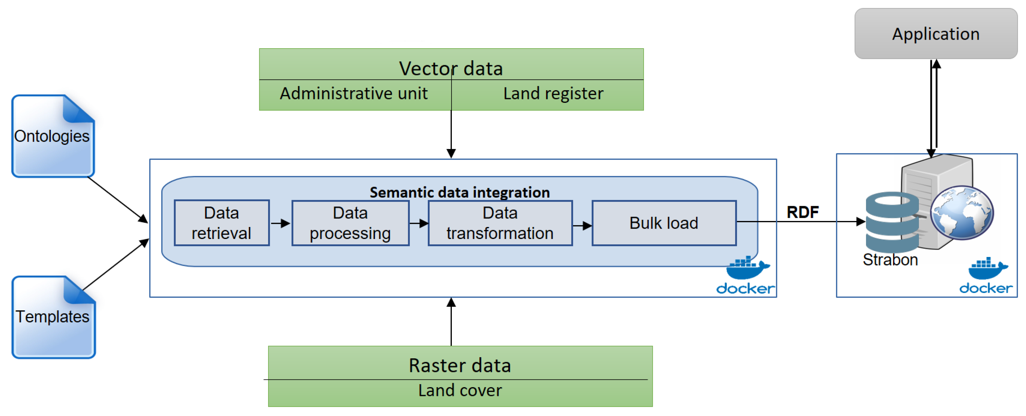
  • As a second contribution, we defined a configurable semantic Extraction, Transformation, and Load (ETL) process based on the proposed model. As in [5], the extraction process starts by linking parts of the data sources schema with concepts and properties in the data model. Hence, we defined a set of transformation functions to populate the semantic model with data (represented as values) and get a homogeneous semantic data representation. One of the features of the integration process is to extract and aggregate data from rasters together with data from other sources. Then, it links the extracted data to the concepts of the semantic model and assigns it spatio-temporal dimensions, thanks to which all data can be linked and queried. This process is reproducible, as it is accessible via a docker image (https://hub.docker.com/r/h2020candela/triplification).
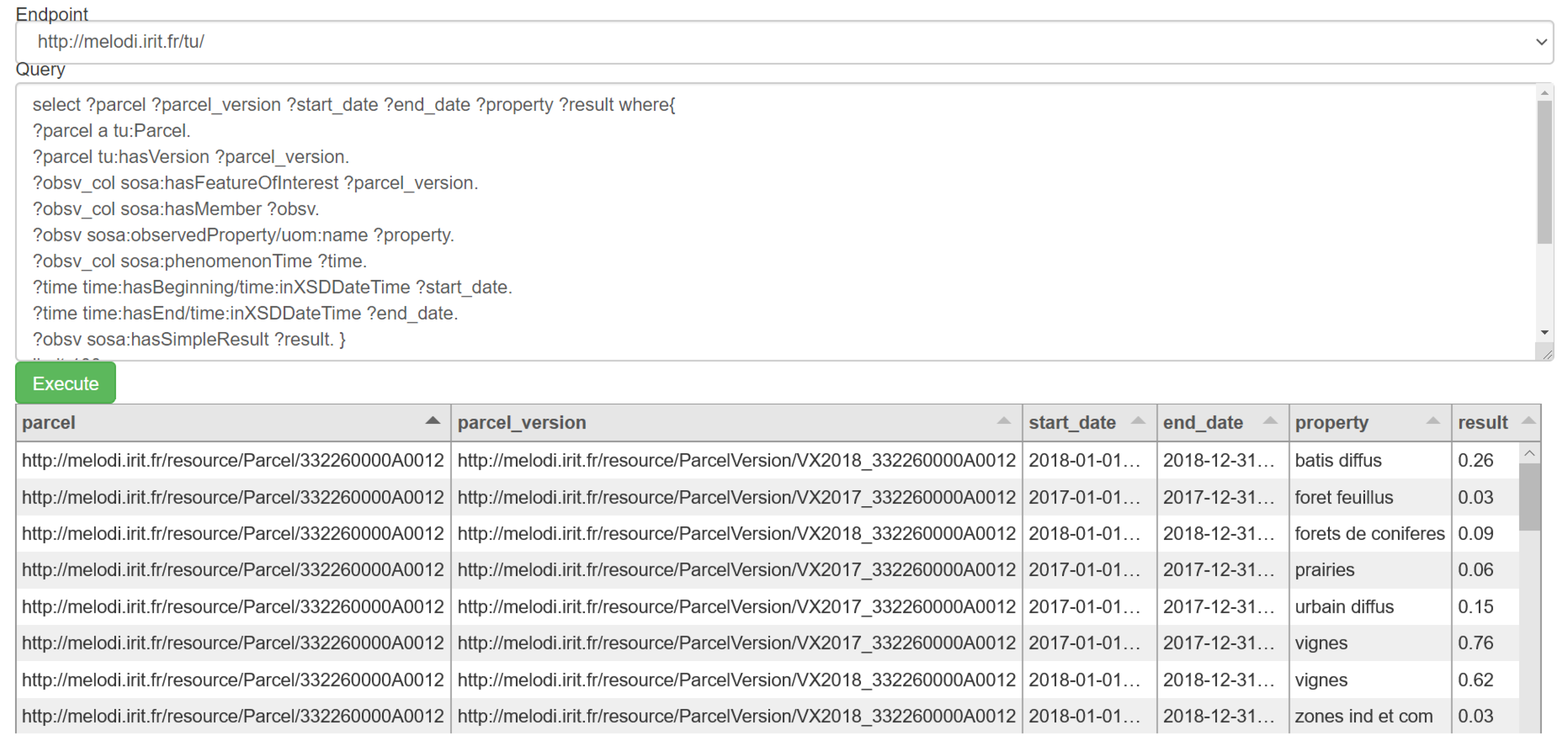
  • A third contribution is the dataset resulting from the integration process of three different sources that we used for experimental validation: land cover data of a specific French winery geographic area, its administrative units, and their land registers. Stored and published as an RDF triplestore, it is exposed through a SPARQL endpoint and exploited by a semantic query interface. Given a period and a village name or a geographic area defined by its geometry, one can retrieve the land registers in this area and the evolution of their land cover during this period. These data serve as the basis for three scenarios: integration of time series observations; EO process guidance; and data cross-comparison.
This work extends the work in [6] by (a) representing the metadata and provenance of the data sources using the DCAT and PROV-O vocabularies, and the data themselves by extending the SOSA vocabulary; (b) considering data extracted from rasters as observable properties, which makes the model generic enough for accommodating any kind of properties (e.g., land cover, change indicator, or vegetation index) as long as they are available in raster format.
This work is carried out in the context of the CANDELA project (http://www.candela-h2020.eu/) that aims at providing building blocks and services allowing users to quickly use, manipulate, explore, and process Copernicus data together with large sets of open data. One of the motivations to build such a platform is that searching for images using only their original meta-data, mainly using the sensor type, the capture date, and the location is not sufficient to find relevant images for a specific purpose. Contextual information, coming from different heterogeneous data sources, such as rasters, may be useful as well as a semantic search module.
The paper is organized as follows. Section 2 discusses the main related work. Section 3 presents the semantic model to integrate data extracted from rasters with geographic data, through their spatial and temporal dimensions. Section 4 details the chosen data sources and the semantic data integration process. Section 5 presents the results and a discussion in terms of applicability of the resulting dataset in different use cases. Finally, Section 6 concludes the paper with perspectives for future work.

2. Related Work

2.1. Semantic Models and Semantic ETL Processes for EO Data Integration

Different semantic ETL proposals have addressed the transformation and integration of (open) EO data to Linked Open Data (LOD). As introduced before, this process is generally guided by a semantic model to get a homogeneous data representation. Most of these models reuse standard semantic web vocabularies, and, more recently, results from multi-dimensional data management like data cubes. In [7], the authors model EO imagery as a data cube with a specific place and time as dimensions—an important break-through for the spatio-temporal web of data [7]. For that purpose, in 2017, the W3C proposed the RDF Data Cube (QB) ontology [8] which has been adopted in many proposals. QB combines standard vocabularies such as the Sensor Network (SSN), OWL-Time, Simple Knowledge Organization System (SKOS) and PROV-O. In [9], QB has been used for publishing tabular time series data and for structuring it into slices to support multiple views on the data. In a way similar to a spatio-temporal data cube, the semantic EO data cube [10] contains EO data where for each observation at least one nominal (i.e., categorical) interpretation is available. Closer to our work but with an ontology-based data access (OBDA) approach, the model used in [11] extends three ontologies, namely Data Cube, GeoSPARQL, and OWL-Time, to offer access to Copernicus services. Rather, we have chosen SOSA to represent observation collections but alignments (https://www.w3.org/TR/vocab-ssn/) exist between SOSA and QB vocabularies to describe observations as multi-dimensional data according to a data cube model.
While some approaches aim at producing open linked datasets, other ones focus on the methodological aspects of interlinking heterogeneous data, as for sensor data products, as discussed in [12]. Several ontologies have been interlinked to create the satellite INSAT-3D vocabulary. In [13], data-intensive environmental services are proposed based on EO data and data from government databases, national and European agencies.
Our approach here is close to these studies in the sense that we guide the integration process on the top of an ontology reusing existing standards. Another close proposal is the one from [3], which carries out an ETL process to integrate EO image and external data sources, such as CLC, Urban Atlas, and Geonames. The process relies on their SAR ontology. Another similar work in terms of datasets is from [14], where data is integrated and published as LOD based on an ontology, called proDataMarket. Three data sources, the Spanish land parcel identification system, Sentinel-2 satellite, and LiDAR flights, are integrated. In [15], satellite images are classified and enriched with semantic data to enable queries about what can be found at a particular location. Our work shares a similar solution to reach the same goal with different types of data.
Several works address the issue of managing large volumes of EO data. For instance, in [16] a framework helps to integrate and process large-scale heterogeneous data generated from multiple sources to support decisions that would prevent natural disasters. The semantic integration of EO and non-EO data is based on the MEMOn modular ontology that reuses the BFO, CCO, SSN, and ENVO ontologies.

2.2. Processing of Raster Data in a Semantic Framework

We can distinguish two approaches for raster data representation that match two traditional ways of processing raster data: processing the entire raster grid as coverage or providing procedures to extract vector objects from the raster matrix. The first option relies on a semantic representation of the raster pixels so that each pixel attribute (geometry, values) is maintained. [17] designed the RDF Grid coverage ontology to support a native integration of coverage in RDF triplestores. The gridded structure of the data is preserved and can be queried using SciSPARQL. Recently, the Ontop-spatial extension [18] can process raster data and create virtual geospatial RDF views above them. The tool automatically translates each raster pixel into a feature thanks to mapping declaration and the polygon dumping function of PostGIS. The raster must consequently be imported into a PostGIS database before processing. In this approach, converting the all raster pixels into RDF significantly increases the number of triples, which in the end might cause performance issues.
The second approach consists of extracting entities from raster files and representing them as ontological features. These entities are sets of raster elements (i.e., sets of pixels) that meet a certain context-dependent definition. A prototype is presented in [19] to integrate and process scientific vector and raster data from LOD repositories using vectorization and mathematical tools for geo-processing. First, bounding boxes from raster are used to query LOD endpoints for geofeatures. Next, the returned geofeatures are used to select raster pixels for supervised training based on content-based descriptors. Finally, the results can be vectorized, transformed, and inserted into the triplestore. In [3], the approach proposes to restructure the images in patches with a fixed size, to which contextual information is linked. In the end, each patch is directly transformed into a feature based on their ontology. A similar solution is implemented in [20] where the ontological features are road segments. By mapping their bounding boxes (1 meter around the segment) to the raster data, the pixel value in this area is compared to a threshold and determines the value of a semantic property of the road segment. The authors also propose to extend the SPARQL query language so as to manage standard geometric functions on both raster files and vector files. To do so, they polygonize the desired region of the raster. This workaround is arguably not a complete solution to represent raster files in RDF as the original geometric source of the data is not preserved [21]. In our approach, the areas of interest are predefined, hence the geometries (polygons) are known.

2.3. Positioning Our Contribution

In Table 1, we compare our model with the closest state-of-the-art ones for EO data representation or integration. We consider a model as published when it is publicly available or when it is well described in a companion document (article or website) or with the help of rich metadata. The model is said to be reusable when it is generic enough to be used in other scenarios or systems. In the comparison table, we reported the properties of each model, included ours. Our model satisfies all the needs required for a richer and open model; it is published, reusable, and supports temporal dimension as well as source metadata; moreover, it is one of the few models able to represent raster data.
Table 2 presents a comparison of our proposal to the closest ones in the literature for raster integration or representation. The most similar approach that makes use of vector input (containing geolocated features) is [19]. However, this work is not completed and the model has not been published.
In Table 2 we distinguish two ways of performing semantic data integration: either a mediator is built for virtual systems (on-demand mapping) or data materialization is accomplished for persistent systems (data materialization). These are important aspects of the ETL process. For the on-demand mapping, data remains located in their source, as a consequence, SPARQL queries must be rewritten at the query evaluation step. This approach is well-suited in the context of very large datasets that would hardly support centralization due to resource limitations. For data materialization, like in warehouse approaches, data sources are transformed into RDF graphs that are thereafter loaded into a triplestore and accessed through a SPARQL query engine. Our proposal applies the materialization approach. The major advantage of this approach is to facilitate further processing, analysis, or reasoning on the materialized RDF data. More specifically, this choice is motivated by the following reasons: (i) it is not easy to run an on-demand mapping since the data sources we considered (presented below) are available in different formats (JSON/GeoJSON, GeoTIFF image, shapefile or even remote compressed files), which requires a pre-processing step of conversion; (ii) Geospatial triplestores can be considered as a warehouse to store semantic data so that data enrichment and linking could be performed; and (iii) different datasets may be offered by different endpoints requiring federation mechanisms, however, there is currently no query engine mature enough for answering GeoSPARQL queries over such a federation [11]. As we send a single GeoSPARQL query to examine the geofeatures stored in different places, spatial comparisons on the fly are not possible.

3. Semantic Models for EO Data Integration

We aim at integrating data sources using their spatio-temporal dimensions. In other words, given areas of interest, such as territorial units or agricultural parcels, and data sources, we want to build a knowledge graph that links the appropriate data to each unit. Our approach relies on a semantic model that provides a unique vocabulary to represent all the data and the territorial units. We designed this model as a generic and modular ontology that reuses standard vocabularies. To build the first module, called Territorial Unit Model (TUM), we reused and extended the TSN ontology (Territorial Statistical Nomenclature ontology) [22] that represents areas of interest, such as administrative units and parcels, along with their versions. To represent observations made on a given area and for a period, we defined a second module, the TUOM ontology (Territorial Unit Observation Model ontology). An observation can be seen as an activity producing a calculated property value of the areas. Before presenting the TUM and TUOM models (Section 3.2), we describe the state-of-the-art vocabularies on which they rely (Section 3.1), namely GeoSPARQL (for geospatial data), OWL-Time (for temporal features), DCAT (for data sources metadata), PROV-O (for data sources provenance) and SOSA (for the observations).

3.1. Reused Vocabularies

3.1.1. Standard Vocabularies

GeoSPARQL ontology (https://www.ogc.org/standards/geosparql): the GeoSPARQL ontology (extract presented in the top-left box of Figure 1), an OGC standard, introduces the geo:SpatialObject class composed of two primary subclasses, geo:Feature and geo:Geometry [23]. The first one represents an entity of the real world while the latter represents all geometric forms defined on a spatial coordinate reference system. An entity is associated with its geometries by the geo:hasGeometry relation. GeoSPARQL provides topological relations and functions to link spatial objects (intersects, touches, etc.).
OWL-Time ontology (https://www.w3.org/TR/owl-time/): the OWL-Time ontology (top-right box of Figure 1) [24] is recommended by the W3C for modeling temporal concepts (instants and intervals) and expressing topological relations as defined in the theory of Allen between them (before, after, etc.). It is used to describe the temporal properties of the data.
DCAT vocabulary (https://www.w3.org/TR/vocab-dcat-2/): DCAT is a vocabulary designed to publish metadata catalogs on the web. In DCAT, a catalog (dcat:Catalog) is a dataset in which each item is a metadata record describing some resource; the scope of the catalog is collections of metadata about datasets or data services. A dataset (dcat:Dataset) is a collection of data, published or curated by a single agent. The vocabulary combines elements from other vocabularies such as Dublin Core Terms (dct prefix): dct:temporal and dct:spatial are used to describe the spatial and temporal coverage of the dataset. An instance of the dcat:Distribution class represents a concrete implementation of a dataset (e.g., raster, shapefile, etc.).
PROV-O ontology (https://www.w3.org/TR/prov-o/): PROV-O defines a data model, serializations, and definitions to support the interchange of provenance information on the Web. It is a recommendation of the W3C to allow assessments about the quality, reliability, or trustworthiness of data. In this vocabulary, an entity (prov-o:Entity) is something that may be derived from other entities.
SOSA ontology (https://www.w3.org/TR/vocab-ssn/): the SOSA ontology (Sensor, Observation, Sample, and Actuator) [25] is a light-weight but self-contained core ontology representing elementary classes and properties of the ontology SSN (Semantic Sensor Network). It describes sensors, their observations and their procedures, and has been largely adopted in a range of applications, and more recently, in satellite imagery. In the SOSA vocabulary, an observation (sosa:Observation) is considered as an activity providing an estimation of a property value using a given procedure. It allows us to describe the related feature of interest and the observed property as well. SOSA reuses OWL-Time to date observations (sosa:phenomenomTime). The sosa:ObservationCollection class is an extension proposed in a current working draft (https://www.w3.org/TR/2020/WD-vocab-ssn-ext-20200116/). It represents a collection of observations that share a common value for one or more of the observation properties (e.g., same sensor, same scene). Such a representation avoids the duplication of triples, and as a consequence, it optimizes data storage and reduces query execution time.

3.1.2. Other Vocabularies

The TSN ontology (Territorial Statistical Nomenclature ontology [22], presented by the top-middle box in Figure 1) describes any territorial nomenclature throughout time (i.e., it permits versions of nomenclatures). The TSN ontology adopts the perdurantist approach of ontologies for fluent [26] to describe the TSN elements that vary in time; however, the authors prefer to use the term Version while other ontologies, for fluency, use TimeSlice. As territorial unit versions represent entities geo-localized at a given time, the ontology reuses the GeoSPARQL and the OWL-Time ontologies.

3.2. Integration Ontology

The integration ontology is modular: each module forms an independent model with a limited number of relations with concepts of other modules.

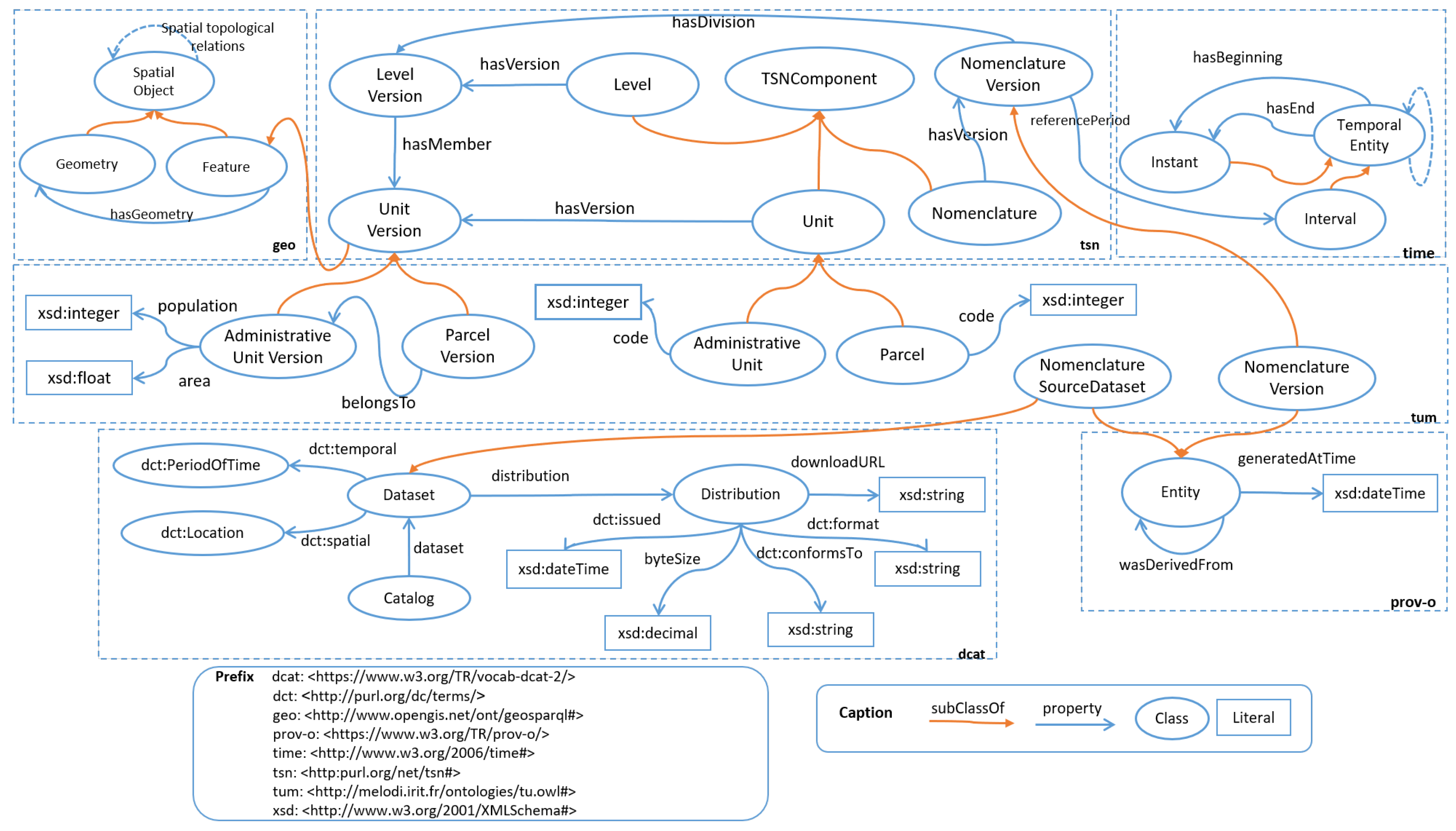
3.2.1. Territorial Unit Model (TUM)

To represent different kinds of territorial units, such as administrative units and parcels, throughout their life, we propose the Territorial Unit Model (TUM) ontology that extends the TSN ontology described above. Indeed, since administrative units and land registers datasets are updated regularly, it is possible to manage different versions of their content. TUM introduces two classes, tum:AdministrativeUnit and tum:Parcel. They extend the tsn:Unit to take into account different timeslices of these entities through time. We use the PROV-O vocabulary for the management of the integrated sources. A territorial unit nomenclature version is thus considered as a prov-o:Entity that was derived from an (open) dataset, i.e., an another prov-o:Entity. This source (tum:NomenclatureSourceDataset) is also represented as a dcat:Dataset whose distribution is in most cases a vector file containing geofeatures.

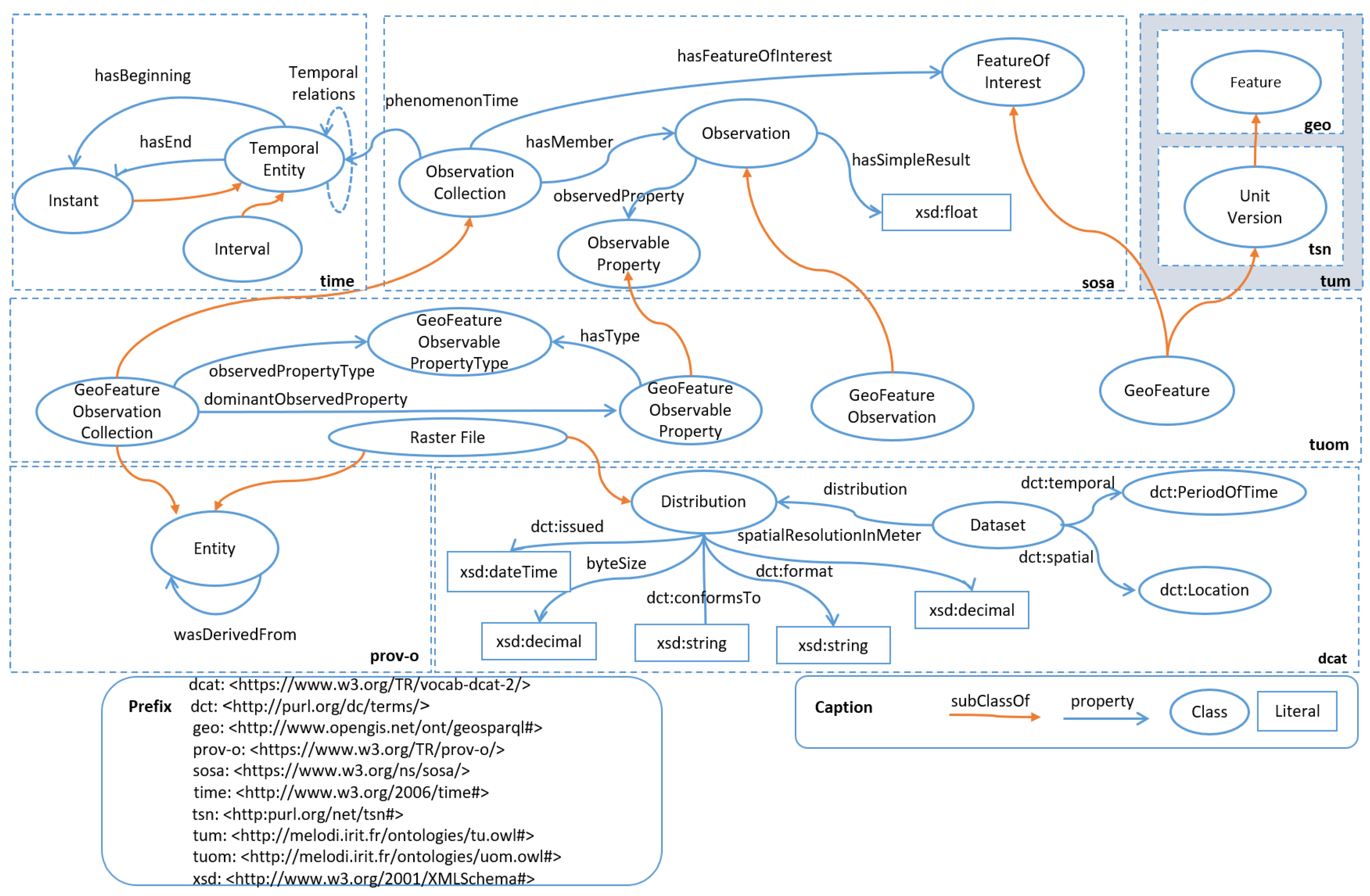
3.2.2. Territorial Unit Observation Model (TUOM)

To represent observations made on territorial units (e.g., land cover, change indicator, or NDVI), we have defined the TUOM ontology (Territorial Unit Observation Model ontology). This ontology (Figure 2) relies on SOSA for describing observations on the units. Each observed property (e.g., the Water or Vineyards class of the CESBIO-LC) is represented as a tuom:GeoFeatureObservableProperty and belongs to a tuom:GeoFeatureObservablePropertyType (e.g., the CESBIO-LC 2018). A tuom:GeoFeatureObservationCollection groups all the observations collected for the same property type from the same raster (temporal dimension) and for the same territorial unit (spatial dimension). A percentage value is attributed to each observation as the result measured for an observed property. For example, 25% of Water and 75% of Vineyard. To reduce query complexity and time processing, we also compute the dominant property tuom:dominantObservedProperty of the observation collection.

4. Semantic Integration Process

The semantic integration process can be divided into several steps, as in an ETL process. This process relies on the definition of semantic mappings, by identifying the parts of the data sources schema which are related to the semantic data model, supporting the extraction process; and on the definition of transformation functions for populating the data modules with homogeneous values.

4.1. Data Sources

We distinguish two kinds of data sources: (i) vector data with a geospatial component corresponding to the zones which one wishes to qualify from raster data (e.g., territorial units or land registers); (ii) rasters with their metadata (date, footprint and the corresponding classification).
  • Vector data sources: Vector data sources contain geofeatures with a geometry. We consider the two following vector data sources to produce our RDF dataset.
  • Raster data sources: A raster data source provides a matrix of cells (or pixels) where each cell contains a value representing the phenomenon considered by the source. Each cell covers a portion of the Earth’s surface; the size of the cells is defined by the spatial resolution of the raster. Higher spatial resolution involves more cells per unit area. When cells contain class values (e.g., land cover class), the classification must be provided to decode these values.
    Raster is the standard format of interchange between tools developed in the project, including tools for change detection and land cover classification from Sentinel images. Other formats will be considered in the next development. Our RDF dataset provides data computed from land cover rasters.
    • Land cover rasters: Each pixel of land cover rasters provides information about the physical coverage of the Earth’s surface at this place. Coverage may be over forests, grasslands or croplands for instance. Each type of cover is associated with a number according to the specific classification, and the pixel value is set to one of these numbers. There are different sources of land covers, with their classification. A global-scale source is GLC-SHARE (http://www.fao.org/geospatial/resources/detail/en/c/1036591/), created by FAO in 2012, provided in raster format as GeoTIFF files. CLC datasets (https://www.data.gouv.fr/en/datasets/corine-land-cover-occupation-des-sols-en-france) are based on the CLC vocabulary (http://dd.eionet.europa.eu/vocabulary/landcover/clc). The two most recent ones were published for 2012 and 2018. A more specific French land cover is that of CESBIO (http://osr-CESBIO.ups-tlse.fr/~oso/). A new version is provided yearly, starting from 2016 (dataset for 2009, 2010, 2011, and 2014 are also available) in raster format as a GeoTIFF file. In particular, CESBIO-LC is mainly based on Sentinel-2 images acquired all year long, whereas GLC-SHARE combines various EO sources. Moreover, while the GLC-SHARE has global coverage, with a spatial resolution of 1000 m 2 per pixel, CESBIO-LC only covers France with a spatial resolution of 10 m 2 . We selected the CESBIO datasets and the corresponding land cover classification because of its high-quality.

4.2. Semantic ETL Process

We defined a four-step semantic ETL process to build an RDF triplestore from heterogeneous data sources:
  • Data retrieval: At this step, the datasets of interest are identified according to spatial and temporal criteria and retrieved using dedicated search mechanisms. This step can be done in a semi-automatic way with the help of dedicated scripts. For example, the dataset containing information of a French village can be retrieved based on its INSEE code and the publication year. In the case of land cover rasters, a detailed description of the land cover classes used to code the raster must also be retrieved. Such a vocabulary is usually described by a text (CESBIO-LC) or PDF file (CLC or GLC-SHARE).
  • Data extraction: This step aims at extracting and structuring data from the data sources. Firstly, metadata (e.g., issue date, format, CRS, or spatial extent) is extracted. The, entity geometry in vector files is matched to the WGS84 CRS, which is the default CRS of GeoSPARQL. Rasters are processed to qualify territorial units: either new properties (e.g., mean values) are extracted through pixel aggregation or a spatial mask is used to eliminate undesired areas (i.e., only the area inside the unit footprint is preserved). For example, the land cover of a parcel is computed from a raster in three steps:
    (a)
    Reproject the parcel and the land cover raster onto the same CRS.
    (b)
    Apply the parcel (the geometry of the parcel version at a given date) as a mask on the raster.
    (c)
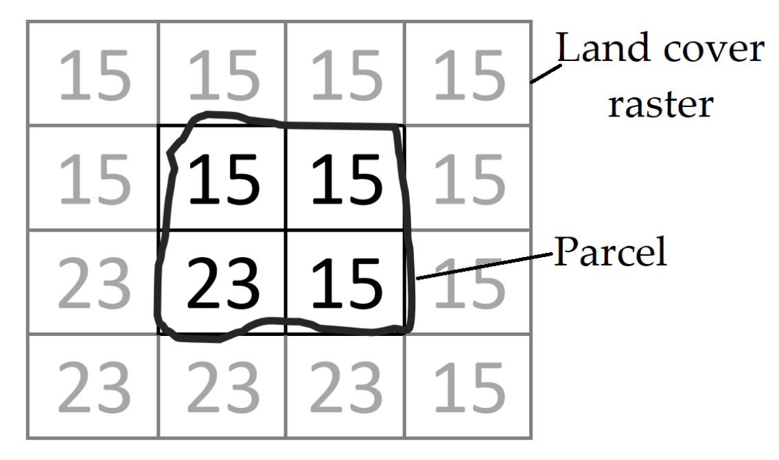
    Calculate the percentage of each land cover class occupying the parcel. For example in Figure 3, the parcel covers four pixels: three of them are annotated as vineyards (code 15), the last one is water (code 23). In other words, 75% of the parcel are vineyards and the rest is water.
    The result of this step is a temporary JSON structure that is used for transformation at the next step. We chose JSON because it can describe both observations and geospatial features.
  • Data transformation: This step aims at transforming the processed data into a semantic one. Templates defining the mapping between the source schema and the ontologies are used as a basis in this process. They are usually handwritten and make the mappings explicit. Data translation tools, such as D2RQ (http://d2rq.org/), Ultrawrap (https://capsenta.com/ultrawrap/), Morph (http://mayor2.dia.fi.upm.es/oeg-upm/index.php/en/technologies/315-morph-rdb/), Ontop (http://ontop.inf.unibz.it/), or GeoTriples (http://geotriples.di.uoa.gr/) using such mappings can be used. However, we have chosen to evolve the mapping template and processing mechanism of our recent work [27] because more functions can be added to perform more sophisticated operations that are not possible in alternative approaches. The output of this step is a set of RDF files.
    At this step, the land cover classification (class codes and label) is also transformed into RDF as instances of two classes: tuom:GeoFeatureObservablePropertyType and tuom:GeoFeatureObservableProperty. The transformation process takes as input the classification described by a CSV structure composed of two columns (code and label) and can be independently performed with the one for raster. Appendix A is an example of JSON structure extracted at the previous step.
    Appendix B presents an extract of the templates used to transform extracted information into RDF format. In these templates, the valueToLiteral function is used to transform a value to literal and the $Instance_X keyword is used to automatically initiate an instance of class X by defining its URI. The variables (begin with $.) represent the values of the JSON representation.
    Appendix C lists some RDF triples generated from the JSON structure presented in Appendix A using the above templates.
  • Data load: the final step consists of importing the RDF files into the triplestore.

4.3. System Architecture

The system is developed through docker technology. There are two dockers as described in Figure 4: the first one contains Python scripts for data retrieval, data processing, data transformation, and triplestore bulk load, the second one is used to deploy the geospatial triplestore that manages the knowledge base.
Currently, several triplestores support storing and querying spatial data using GeoSPARQL or stSPARQL. Those free that offer a good support are Parliament (http://parliament.semwebcentral.org/) [28], Strabon (http://strabon.di.uoa.gr/) [29] and GraphDB (http://graphdb.ontotext.com/). They explicitly adopt the existing geospatial geometry standard, although many triplestores now support spatial queries of different complexity [30]. While we have not tested Parliament, we did for GraphDB that performed poorly for the queries involving spatial joins. Strabon has hence been chosen in our project as it has many advantages:
  • Strabon extends the Sesame triplestore with the capacity of storing spatial RDF data in the PostgreSQL DBMS enhanced with PostGIS. The triplestore has a good overall performance thanks to particular optimization techniques that allow spatial operations to take advantage of PostGIS functionality instead of relying on external libraries [31]. For complex applications that include both spatial joins or spatial aggregations, Strabon is the only RDF store that performed well [32].
  • Strabon also provides a SPARQL endpoint that helps to access the content of the triplestore. The interface also provides an additional possibility to manage the knowledge base, for instance storing and updating functionalities with SPARQL Update.
The first docker containing the ETL process is publicly available here (https://hub.docker.com/r/h2020candela/triplification). The second docker containing Strabon can be found on-line (https://hub.docker.com/r/bde2020/strabon).

5. Results and Discussion

The results are evaluated with regards to the contributions of the resulting dataset to three use cases: integration of time series observations; EO process guidance; and data comparison. The areas of interest were chosen to answer to data requirements in the CANDELA project supporting different kinds of analysis from change detection to land cover evolution. The resulting dataset allows for users to homogeneously query the data, helping their tasks of information retrieval. Serving different use cases corroborates the contribution of our proposal in terms of a modular ontology that can accommodate different kinds of EO properties extracted from rasters along their spatial and temporal dimensions.
The resulting semantic data was stored in a database that can be accessed through a semantic search interface or via a SPARQL endpoint (http://melodi.irit.fr/tu/). The triplestore contains information about the French villages and their 2017 and 2018 versions. Out of 1377, 58 villages which are inside the zone of study (French departments 24, 33 and 47), were associated with parcel versions. The whole set results in 224,000 parcels (instances of tum:ParcelVersion) in the database. The CESBIO-LC information (2017 and 2018) is being updated based on the use cases and the user’s need for analysis. While query performance is not optimal in the current publicly available version of the RDF dataset, performance and scalability have to be addressed in the future. An extended version of the dataset (including parcels and administrative units from other French departments) will be deployed on the CANDELA project platform.
We present in the following paragraphs a basic user interface that allows for querying the dataset via SPARQL queries and visualizing the results with the help of a map. End-users evaluated the dataset in terms of its content rather than the interface provided for querying it. While the use cases discussed below are specific to the project needs, the dataset can potentially be useful for the community as it repertories all the parcels, administrative units and their versions for a specific area in France.

5.1. Integration of Time Series Observations

The resulting dataset provides information about parcels and administrative units (villages) of the three French departments. It also contains the details of the processed rasters. Users can make use of the knowledge base to monitor the land cover change through time. This can be done by examining all observations made on all parcel versions or administrative units. An example of a query involving parcels and its results is illustrated in Figure 5. It is observable that the land cover of the parcel 332260000A0012 has slightly changed between 2017 and 2018: vineyard decreased from 76% to 62% while urban fabric increased from 15% to 26%.
As we keep track of the data provenance and the source metadata, it is possible to retrieve the details of the origin of the raster that has been used to generate an observation. Figure 6 presents a query for raster used to compute observations made on the parcel in 2017 (a tuom:GeoFeatureObservationCollection). Reversely, it is also possible to retrieve all the observations generated from a given raster.

5.2. EO Process Guidance

The dataset can also be exploited in diverse EO analysis processes. On the one hand, one can apply a set of algorithms on the returned query results, that contain spatial and temporal information (the parcels or related Sentinel images; and the period, respectively). On the other hand, the returned results can guide and boost the performance of the algorithms by providing precise spatial and temporal parameters (from the results of a query, we know on which region and for which period a specific analysis has to be carried out). It is then possible to make a pipeline combining semantic query with other modules like change detection or NDVI computation.
More concretely, the dataset serves to two use cases of the CANDELA project:
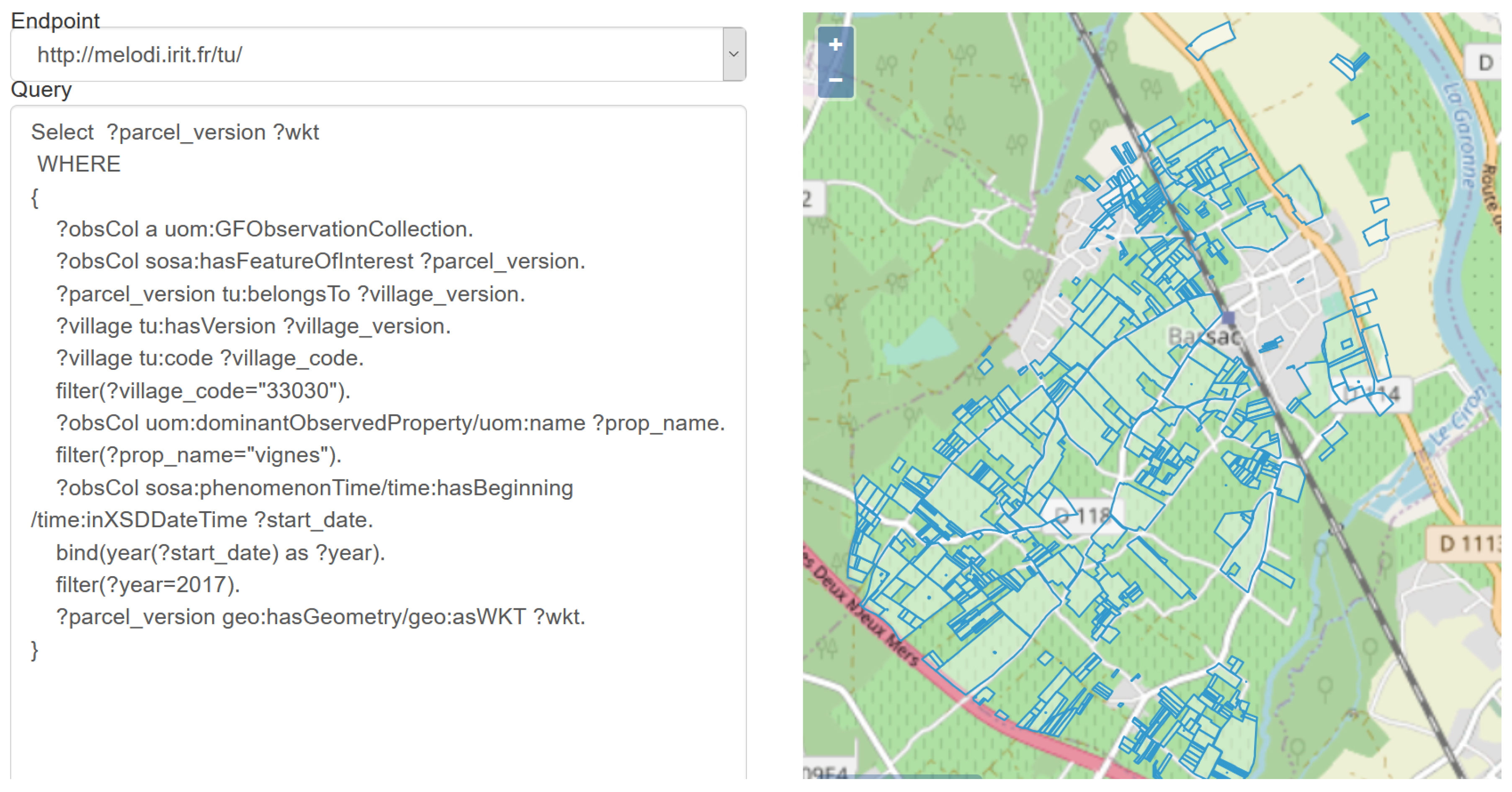
  • Change detection in vineyards: the use case aims to detect changes in vineyard vegetation due to natural hazards such as frost or hail. The semantic database can be used to retrieve and locate vineyard parcels through time. Figure 7 illustrates the query and resulting data when querying all vineyard parcels of the Barsac village (code 33030) in 2017. The vineyard parcels are displayed on the map. Having identified the vineyard parcels, one can retrieve the corresponding images for change detection analysis.
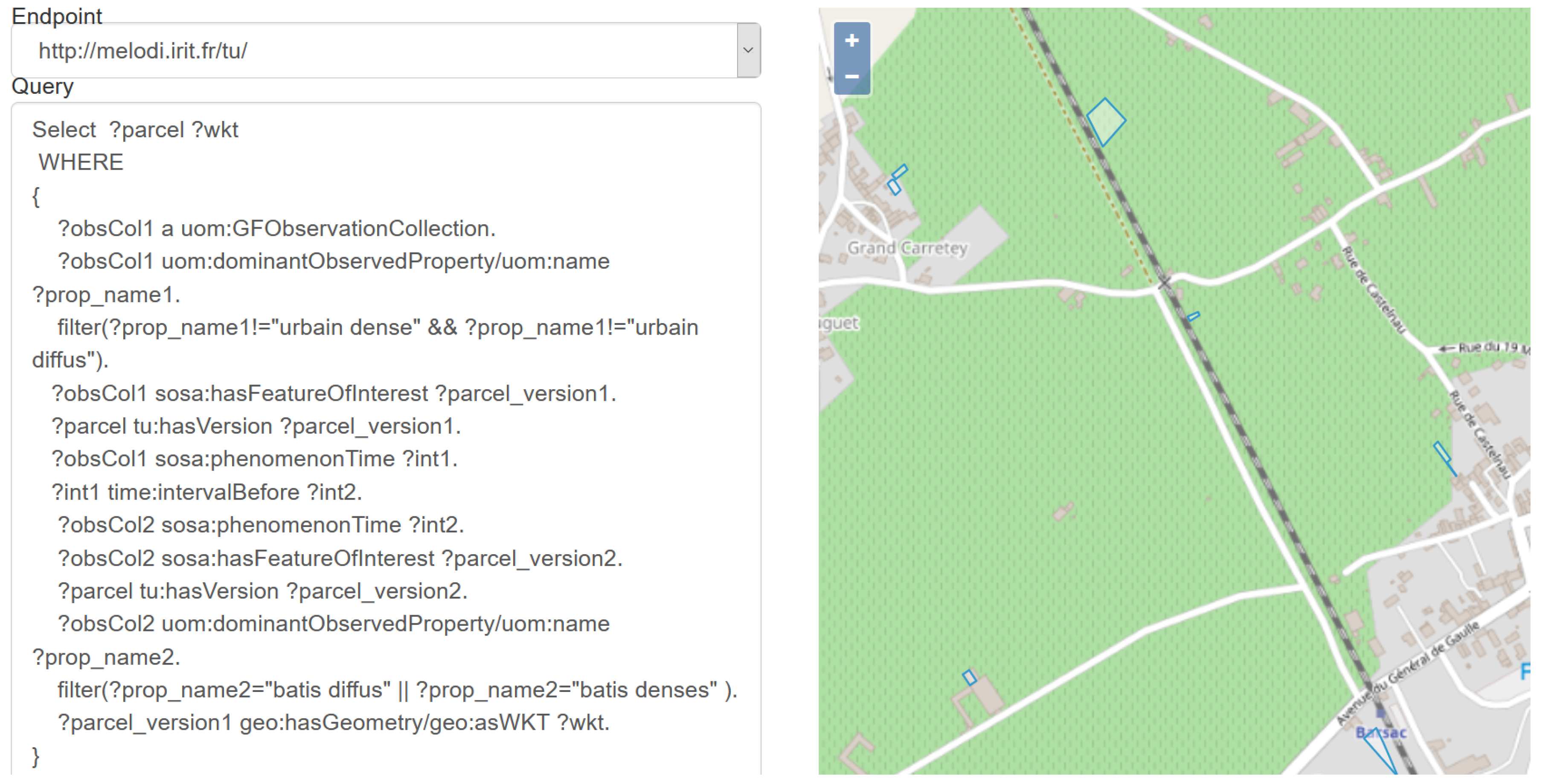
  • Urban expansion and agriculture: the use case studies the effect of urban expansion on agricultural areas due to the continuous development of human settlements. Additionally, it tries to analyze the changes in agricultural land covers through time due to the climatic changes that force farmers to shift their crops to achieve higher economic returns. The knowledge base is then exploited as a reference from which agricultural parcels that had been transformed into urban can be queried. Figure 8 demonstrates such a query; transformed parcels located on the northwest of the Barsac village are highlighted on the map (surrounded areas). While this scenario is close to the first use case, here with the land cover indexes being stored for each year, one can identify the parcels that have been impacted by an evolution (land cover evolution).

5.3. Data Cross-Comparison

Another scenarioof exploitation of this dataset is the cross-comparison of information from various sources, including the results provided by the project partners. For example, it is possible to compare the CESBIO-LC information to the land cover annotated by DLR, a project partner; or to explain a change detection from unsupervised machine learning results, as provided by Thalès (another project partner). For the former example, while the results from DLR have not been included yet in the dataset, a manual comparison has been made from what is stored in our dataset and the land cover map generated by DLR.

6. Conclusions

We propose a modular semantic model able to accommodate different dimensions required for representing EO data: time, space, observation, source metadata, and provenance, together with a semantic ETL process for populating this model. We illustrated our approach by the integration of land cover data of a specific French winery geographic area, its administrative units, and its land registers. The feasibility of the approach and the capacity of the system has been demonstrated in the H2020 EO Big Data Hackathon (http://www.candela-h2020.eu/content/joint-hackathon-organized-eo-2-2017-projects). During the event, participants could access the project platform to integrate new land cover datasets and then query the triplestore to retrieve details of the administrative units or the parcels with their land cover. All the tasks are realized through python scripts.
As future work, we will consider other available datasets, such as land use, vegetation index, and change detection. Following the data triplification process that we defined, additional information can be attached to parcels throughout their life so that they can be referred to in the analysis process. We will consider, as well, integrating other land cover datasets, such as the one from [33]. Finally, another direction is to consider big data scenarios (using Natura 2000 data for instance) and to evaluate the scalability of the approach, including the possibility of considering hybrid architecture and storage strategies (with relational, NoSQL and RDF storage supports).

Author Contributions

The authors contributed in the following way to the work reported in this paper and to its writing: conceptualization and methodology, Nathalie Aussenac-Gilles, Catherine Comparot, Ba-Huy Tran and Cassia Trojahn; software, Ba-Huy Tran; validation, Ba-Huy Tran and Catherine Comparot; formal analysis, Ba-Huy Tran and Cassia Trojahn; investigation, Nathalie Aussenac-Gilles, Catherine Comparot, Ba-Huy Tran and Cassia Trojahn; resources, Catherine Comparot and Ba-Huy Tran; data curation, Ba-Huy Tran; writing—original draft preparation, Catherine Comparot, Ba-Huy Tran and Cassia Trojahn; writing—review and editing, Nathalie Aussenac-Gilles, Catherine Comparot, Ba-Huy Tran and Cassia Trojahn; visualization, Nathalie Aussenac-Gilles and Ba-Huy Tran; supervision, Nathalie Aussenac-Gilles, Catherine Comparot, and Cassia Trojahn; project administration, Nathalie Aussenac-Gilles, Ba-Huy Tran and Cassia Trojahn; funding acquisition, Nathalie Aussenac-Gilles and Cassia Trojahn. All authors have read and agreed to the published version of the manuscript.

Funding

This work benefited the financial supports of an H2020 EC research grant for the CANDELA project under convention 776193.

Conflicts of Interest

The authors declare no conflict of interest.

Appendix A. Data Extraction

At the data extraction step, raster data is extracted. Below is a (simplified) result representing the observations.
{
           "type": "LC_CESBIO",
    "raster": "LC_CESBIO_OCS_2017_CESBIO_tile",
           "foi": "VX2017_330300000A0480",
    "startDate": "2017-01-01",
    "endDate": "2017-12-31",
    "observations": [{
            "property": 11,
            "result": 0.1
           },
           {
            "property": 31,
            "result": 0.9
           }
           ]
}
		

Appendix B. Data Transformation Templates

At the data transformation step, a template is used to transform extracted data into RDF format. An extract of each template is presented below.

Appendix B.1. Template for Administrative Unit Dataset

           $Instance a tum:AdminUnit.
           $Instance tum:code valueToLiteral($.insee, string).
           $Instance tum:hasVersion $Instance_AdminUnitVersion.
    $Instance_AdminUnitVersion a tum:AdminUnitVersion.
    $Instance_AdminUnitVersion tum:name valueToLiteral($.name, string).
    $Instance_AdminUnitVersion tum:area valueToLiteral($.area, float).
    $Instance_AdminUnitVersion geo:hasGeometry $Instance_Geometry.
           $Instance_Geometry a geo:Geometry.
           $Instance_Geometry geo:asWKT valueToLiteral($.wkt, wktLiteral).
		  

Appendix B.2. Template for Parcel Dataset

           $Instance a tum:Parcel.
           $Instance tum:code valueToLiteral($.id, string).
           $Instance tum:contenance valueToLiteral($.contenance, integer).
           $Instance tum:hasVersion $Instance_ParcelVersion.
           $Instance_ParcelVersion tum:belongsTo valueToInstance($.village,
           AdminUnitVersion)
           $Instance_ParcelVersion geo:hasGeometry $Instance_Geometry.
           $Instance_Geometry a geo:Geometry.
           $Instance_Geometry geo:asWKT valueToLiteral($.wkt, wktLiteral).
		  

Appendix B.3. Template for Land Cover Dataset

           $Instance a tuom:GFObservationCollection.
           $Instance a dcat:Dataset.
    $Instance a prov-o:Entity.
           $Instance tuom:observedPropertyType valueToInstance($.type,
            GFObservablePropertyType).
           $Instance prov-o:wasDerivedFrom valueToInstance($.raster, RasterFile).
           $Instance sosa:hasFeatureOfInterest valueToInstance($.foi, ParcelVersion).
           $Instance sosa:phenomenonTime valueToInterval($.startDate, $.endDate).
           #loop
           $Instance sosa:hasMember $Instance_GFObservation.
    $Instance_GFObservation a tuom:GFObservation.
    $Instance_GFObservation sosa:hasSimpleResult valueToLiteral($.result, float).
    $Instance_GFObservation sosa:observedProperty
                            valueToInstance($.property, GFObservableProperty).
		  

Appendix C. Output RDF Data

Below is an example of semantic data transformed based on the previously presented templates.

Appendix C.1. Administrative Unit Data

:AdminUnit/33030
           a tum:AdminUnit; tum:code "33030"^^xsd:string;
           tum:hasVersion :AdminUnitVersion/V2017_L3_33030.
 
:AdminUnitVersion/V2017_L3_33030
           a tum:AdminUnitVersion; tum:name "Barsac"^^xsd:string; tum:area "1451.0"
           ^^xsd:float;
           geo:hasGeometry :Geometry/V2017_L3_33030.
:AdminUnitVersion/V2018_L3_33030
           a tum:AdminUnitVersion; tum:name "Barsac"^^xsd:string; tum:area "1451.0"
           ^^xsd:float;
           geo:hasGeometry :Geometry/V2018_L3_33030.
:Geometry/V2017_L3_33030 geo:asWKT "POLYGON ((..))".
:Geometry/V2018_L3_33030 geo:asWKT "POLYGON ((..))".
		  

Appendix C.2. Parcel Data

:Parcel/330300000A0480
           a tum:Parcel; tum:code "330300000A0480"^^xsd:string; tum:contenance
           "64120"^^xsd:integer;
           tum:hasVersion :ParcelVersion/VX2017_330300000A0480;
           tum:hasVersion :ParcelVersion/VX2018_330300000A0480.
:ParcelVersion/VX2017_330300000A0480
           a tum:ParcelVersion; tum:belongsTo :AdminUnitVersion/V2017_L3_33030;
           geo:hasGeometry :Geometry/VX2017_330300000A0480.
 
:ParcelVersion/VX2018_330300000A0480
           a tum:ParcelVersion; tum:belongsTo :AdminUnitVersion/V2018_L3_33030;
           geo:hasGeometry :Geometry/VX2018_330300000A0480.
:Geometry/VX2018_330300000A0480 geo:asWKT "POLYGON ((..))".
:Geometry/VX2017_330300000A0480 geo:asWKT "POLYGON ((..))".
		  

Appendix C.3. Land Cover Data

#Land cover observations for 2017
:GFObservationCollection/LC_CESBIO__330300000A0480_1483228800_1514678400
           a tuom:GFObservationCollection; a dcat:Dataset; a prov-o:Entity;
     tuom:observedPropertyType :GFObservablePropertyType/LC_CESBIO;
     prov-o:wasDerivedFrom :RasterFile/LC_CESBIO_OCS_2017_CESBIO_tile;
     sosa:hasFeatureOfInterest :ParcelVersion/VX2017_330300000A0480;
           sosa:phenomenonTime :Interval/1483228800_1514678400;
           sosa:hasMember :GFObservation/LC_CESBIO__330300000A0480_11_1483228800_
           1514678400;
           sosa:hasMember :GFObservation/LC_CESBIO__330300000A0480_31_1483228800_
           1514678400.
:GFObservation/LC_CESBIO__330300000A0480_11_1483228800_1514678400
           a tuom:GFObservation; sosa:hasSimpleResult "0.1"^^xsd:float;
      sosa:observedProperty :GFObservableProperty/LC_CESBIO_11.
 :GFObservation/LC_CESBIO__330300000A0480_31_1483228800_1514678400
           a tuom:GFObservation; sosa:hasSimpleResult "0.9"^^xsd:float;
      sosa:observedProperty:GFObservableProperty/LC_CESBIO_31.
:GFObservableProperty/LC_CESBIO_11 tuom:name "culture ete"^^xsd:string.
:GFObservableProperty/LC_CESBIO_31 tuom:name "foret feuillus"^^xsd:string.
 #Land cover observations for 2018
 :GFObservationCollection/LC_CESBIO18_330300000A0480_1514764800_1546214400
           a tuom:GFObservationCollection; a dcat:Dataset; a prov-o:Entity;
     tuom:observedPropertyType :GFObservablePropertyType/LC_CESBIO18;
     prov-o:wasDerivedFrom :RasterFile/LC_CESBIO_OCS_2018_CESBIO_tile;
     sosa:hasFeatureOfInterest :ParcelVersion/VX2018_330300000A0480;
     sosa:phenomenonTime :Interval/1514764800_1546214400;
           sosa:hasMember :GFObservation/LC_CESBIO18_330300000A0480_10_1514764800_
           1546214400;
           sosa:hasMember :GFObservation/LC_CESBIO18_330300000A0480_16_1514764800_
           1546214400.
:GFObservation/LC_CESBIO18_330300000A0480_10_1514764800_1546214400
           a tuom:GFObservation; sosa:hasSimpleResult "0.12"^^xsd:float;
      sosa:observedProperty :GFObservableProperty/LC_CESBIO18_10.
 :GFObservation/LC_CESBIO18_330300000A0480_16_1514764800_1546214400
           a tuom:GFObservation; sosa:hasSimpleResult "0.88"^^xsd:float;
           sosa:observedProperty:GFObservableProperty/LC_CESBIO18_16.
:GFObservableProperty/LC_CESBIO18_10 tuom:name "mais"^^xsd:string.
:GFObservableProperty/LC_CESBIO18_16 tuom:name "forets de feuillus"^^xsd:string.
		  

References

  1. Villegas, J.; Sánchez Pastor, H.; Hernanz, L.; Checa, M.; Roman, D. Enabling the Use of Sentinel-2 and LiDAR Data for Common Agriculture Policy Funds Assignment. Int. J. Geo-Inf. 2017, 6, 255. [Google Scholar]
  2. Lambin, E.; Geist, H. Land-Use and Land-Cover Change; Springer: Berlin/Heidelberg, Germany, 2006. [Google Scholar]
  3. Espinoza-Molina, D.; Nikolaou, C.; Dumitru, C.O.; Bereta, K.; Koubarakis, M.; Schwarz, G.; Datcu, M. Very-High-Resolution SAR Images and Linked Open Data Analytics Based on Ontologies. IEEE J. Sel. Top. Appl. Earth Obs. Remote Sens. 2015, 8, 1696–1708. [Google Scholar] [CrossRef] [Green Version]
  4. Dumitru, C.; Schwarz, G.; Datcu, M. Land Cover Semantic Annotation Derived from High-Resolution SAR Images. IEEE J. Sel. Top. Appl. Earth Obs. Remote Sens. 2016, 9, 2215–2232. [Google Scholar] [CrossRef] [Green Version]
  5. Bergamaschi, S.; Guerra, F.; Orsini, M.; Sartori, C.; Vincini, M. A semantic approach to ETL technologies. Data Knowl. Eng. 2011, 70, 717–731. [Google Scholar] [CrossRef]
  6. Tran, B.H.; Aussenac-Gilles, N.; Comparot, C.; Trojahn, C. An Approach for Integrating Earth Observation, Change Detection and Contextual Data for Semantic Search. In Proceedings of the International Geoscience and Remote Sensing Symposium (IGARSS), Waikoloa, HI, USA, 19–24 July 2020. [Google Scholar]
  7. Zinke, C.; Ngomo, A.C.N. Discovering and Linking Spatio-Temporal Big Linked Data. In Proceedings of the IGARSS 2018—2018 IEEE International Geoscience and Remote Sensing Symposium, Valencia, Spain, 22–27 July 2018; pp. 411–414. [Google Scholar]
  8. Brizhinev, D.; Toyer, S.; Taylor, K.; Zhang, Z. Publishing and Using Earth Observation Data with the RDF Data Cube and the Discrete Global Grid System; Technical Report; W3C and OGC: Wayland, MA, USA, 2017. [Google Scholar]
  9. Lefort, L.; Bobruk, J.; Haller, A.; Taylor, K.; Woolf, A. A Linked Sensor Data Cube for a 100 Year Homogenised Daily Temperature Dataset. In Proceedings of the 5th International Workshop on Semantic Sensor Networks, Boston, MA, USA, 12 November 2012; pp. 1–16. [Google Scholar]
  10. Augustin, H.; Sudmanns, M.; Tiede, D.; Lang, S.; Baraldi, A. Semantic Earth observation data cubes. Data 2019, 4, 102. [Google Scholar] [CrossRef] [Green Version]
  11. Bereta, K.; Caumont, H.; Daniels, U.; Goor, E.; Koubarakis, M.; Pantazi, D.A.; Stamoulis, G.; Ubels, S.; Venus, V.; Wahyudi, F. The Copernicus App Lab project: Easy Access to Copernicus Data. In Proceedings of the 22nd International Conference on Extending Database Technology (EDBT), Lisbon, Portugal, 26–29 March 2019. [Google Scholar]
  12. Abburu, S.; Dube, N.; Nayak, M.R.; Golla, S. An Ontology Based Methodology for Satellite Data Semantic Interoperability. Adv. Electr. Comput. Eng. 2015, 15, 105–110. [Google Scholar] [CrossRef]
  13. Blower, J.; Clifford, D.; Goncalves, P.; Koubarakis, M. The MELODIES project: Integrationg diverse data using linked data and cloud computing. In Proceedings of the 2014 conference on Big Data from Space (BiDS’14), Frascati, Italy, 12–14 November 2014; pp. 244–247. [Google Scholar]
  14. Sukhobok, D.; Sanchez, H.; Estrada, J.; Roman, D. Linked Data for Common Agriculture Policy: Enabling Semantic Querying over Sentinel-2 and LiDAR Data. In Proceedings of the ISWC 2017 Posters & Demonstrations and Industry Tracks co-located with 16th International Semantic Web Conference (ISWC 2017), Vienna, Austria, 23–25 October 2017; Available online: http://ceur-ws.org/Vol-1963/##paper559 (accessed on 20 August 2020).
  15. Alirezaie, M.; Kiselev, A.; Längkvist, M.; Klügl, F.; Loutfi, A. An Ontology-Based Reasoning Framework for Querying Satellite Images for Disaster Monitoring. Sensors 2017, 17, 2545. [Google Scholar] [CrossRef] [PubMed] [Green Version]
  16. Masmoudi, M.; Taktak, H.; Ben Abdallah Ben Lamine, S.; Boukadi, k.; Karray, M.H.; Baazaoui Zghal, H.; Archimede, B.; Mrissa, M.; Guegan, C.G. PREDICAT: A Semantic Service-Oriented Platform for Data Interoperability and Linking in Earth Observation and Disaster Prediction. In Proceedings of the SOCA 2018: The 11th IEEE International conference on service oriented computing and applications, Paris, Fance, 20–22 November 2018; pp. 194–201. [Google Scholar]
  17. Andrejev, A.; Misev, D.; Baumann, P.; Risch, T. Spatio-Temporal Gridded Data Processing on the Semantic Web. In Proceedings of the DSDIS 2015—2015 IEEE International Conference on Data Science and Data Intensive Systems, Sidney, Australia, 13–15 December 2015; pp. 38–45. [Google Scholar]
  18. Bereta, K.; Xiao, G.; Koubarakis, M. Ontop-spatial: Ontop of geospatial databases. J. Web Semant. 2019, 58, 100514. [Google Scholar] [CrossRef]
  19. Arocena, J.; Lozano, J.; Quartulli, M.; Olaizola, I.; Bermudez, J. Linked open data for raster and vector geospatial information processing. In Proceedings of the 2015 IEEE International Geoscience and Remote Sensing Symposium (IGARSS), Milan, Italy, 18–25 July 2015; pp. 5023–5026. [Google Scholar]
  20. Homburg, T.; Prudhomme, C.; Würriehausen, F.; Karmacharya, A.; Boochs, F.; Roxin, A.; Cruz, C. Interpreting Heterogeneous Geospatial Data Using Semantic Web Technologies. In Proceedings of the International Conference on Computational Science and Its Applications, Beijing, China, 4–7 July 2016; pp. 240–255. [Google Scholar]
  21. Nishanbaev, I.; Champion, E.; Mcmeekin, D. A Survey of Geospatial Semantic Web for Cultural Heritage. Heritage 2019, 2, 1471–1498. [Google Scholar] [CrossRef] [Green Version]
  22. Bernard, C.; Villanova-Oliver, M.; Gensel, J.; Dao, H. Modeling Changes in Territorial Partitions over Time: Ontologies TSN and TSN-change. In Proceedings of the SAC’18: The 33rd Annual ACM Symposium on Applied Computing, Pau, France, 9–13 April 2018; pp. 866–875. [Google Scholar] [CrossRef]
  23. Kolas, D.; Perry, M.; Herring, J. Getting Started with GeoSPARQL; Technical Report; OGC: Wayland, MA, USA, 2013. [Google Scholar]
  24. Hobbs, J.R.; Pan, F. An ontology of time for the semantic web. ACM Trans. Asian Lang. Inf. Process. 2004, 3, 66–85. [Google Scholar] [CrossRef]
  25. Janowicz, K.; Haller, A.; Cox, S.J.; Phuoc, D.L.; Lefrançois, M. SOSA: A lightweight ontology for sensors, observations, samples, and actuators. J. Web Semant. 2019, 56, 1–10. [Google Scholar] [CrossRef] [Green Version]
  26. Welty, C.; Fikes, R. A Reusable Ontology for Fluents in OWL. In Proceedings of the FOIS 2006: The 4th International Conference on Formal Ontology in Information Systems, Amsterdam, NL, USA, 9–11 November 2006; IOS Press: Baltimore, MD, USA; pp. 226–236. [Google Scholar]
  27. Arenas, H.; Aussenac-Gilles, N.; Comparot, C.; Trojahn, C. Semantic Integration of Geospatial Data from Earth Observations. In Proceedings of the EKAW 2016 Satellite Events—20th International Conference on Knowledge Engineering and Knowledge Management, Bologna, Italy, 19–23 November 2016; pp. 97–100. [Google Scholar]
  28. Battle, R.; Kolas, D. Enabling the Geospatial Semantic Web with Parliament and GeoSPARQL. Semant. Web 2012, 3, 355–370. [Google Scholar] [CrossRef]
  29. Kyzirakos, K.; Karpathiotakis, M.; Koubarakis, M. Strabon: A Semantic Geospatial Dbms. In The Semantic Web ISWC 2012; Springer: Berlin/Heidelberg, Germany, 2012; pp. 295–311. [Google Scholar]
  30. Scheider, S.; Degbelo, A.; Lemmens, R.; van Elzakker, C.; Zimmerhof, P.; Kostic, N.; Jones, J.; Banhatti, G. Exploratory querying of SPARQL endpoints in space and time. Semant. Web 2017, 8, 65–86. [Google Scholar] [CrossRef]
  31. Patroumpas, K.; Giannopoulos, G.; Athanasiou, S. Towards GeoSpatial Semantic Data Management: Strengths, Weaknesses, and Challenges Ahead. In Proceedings of the SIGSPATIAL’14: 22nd SIGSPATIAL International Conference on Advances in Geographic Information Systems, Dallas, TX, USA, 4–7 November 2014; pp. 301–310. [Google Scholar]
  32. Ioannidis, T.; Garbis, G.; Kyzirakos, K.; Bereta, K.; Koubarakis, M. Evaluating Geospatial RDF stores Using the Benchmark Geographica 2. arXiv 2019, arXiv:1906.01933. [Google Scholar]
  33. Dumitru, C.O.; Schwarz, G.; Pulak-Siwiec, A.; Kulawik, B.; Lorenzo, J.; Datcu, M. Earth Observation Data Mining: A Use Case for Forest Monitoring. In Proceedings of the IGARSS 2019—2019 IEEE International Geoscience and Remote Sensing Symposium, Yokohama, Japan, 28 July–2 August 2019; pp. 5359–5362. [Google Scholar]
Figure 1. The Territorial Unit Model ontology to represent territorial units (such as French administrative units and land registry parcels), and their history.
Ijgi 09 00503 g001
Figure 2. The Territorial Unit Observation Model ontology to represent property values of territorial units calculated from EO rasters.
Ijgi 09 00503 g002
Figure 3. An example of parcel masking (15: Vineyard, 23: Water).
Ijgi 09 00503 g003
Figure 4. The system architecture based on docker technology.
Ijgi 09 00503 g004
Figure 5. Monitoring land cover change.
Ijgi 09 00503 g005
Figure 6. Data provenance and source metadata.
Ijgi 09 00503 g006
Figure 7. Location of vineyard parcels (surrounded areas) of the Barsac village in 2017.
Ijgi 09 00503 g007
Figure 8. Location of transformed parcels (surrounded areas), from agricultural land to urban on the north west of the Barsac village between 2017 and 2018.
Ijgi 09 00503 g008
Table 1. Comparison of semantic model for Earth Observation (EO) data integration/representation.
Presented
Work
Main Reused
Ontologies
PublishedReusableTemporalitySource
Metadata
Query
Language
Raster
Support
[3]stModelX stSPARQLX
[11]GeoSPARQL
OWL-Time
Data Cube
XXX GeoSPARQL
[13]stModel X stSPARQL
[14]GeoSPARQL
Data Cube, DUL
XX GeoSPARQL
[15]GeoSPARQL
DUL
GeoSPARQLX
[16]SSN, CCO
BFO, ENVO
XXX SPARQL
[17]noneX SciSPARQLX
[18]GeoSPARQL GeoSPARQLX
[19]GeoSPARQL GeoSPARQLX
[20]GeoSPARQLX GeoSPARQLX
OursGeoSPARQL
OWL-Time
SOSA, PROV-O
TSN
XXXXGeoSPARQLX
Table 2. Comparison of raster integration/representation work.
Presented
Work
Integration ApproachVector
Input
Raster RepresentationStorage
[3]Materialization Entities based extraction (Fixed patches)RDB->Strabon
[15]Unknown Entities based extractionUnknown
[17]Materialization CoverageArray
[18]On-demand mapping CoveragePostGIS
[19]MaterializationXEntities based extractionStrabon
[20]On-demand mapping Entities based extraction (Polygonizing)RDB
OursMaterializationXEntities based extractionStrabon

