An Economic Development Evaluation Based on the OpenStreetMap Road Network Density: The Case Study of 85 Cities in China


Abstract
:1. Introduction
2. Study Areas and Data Source
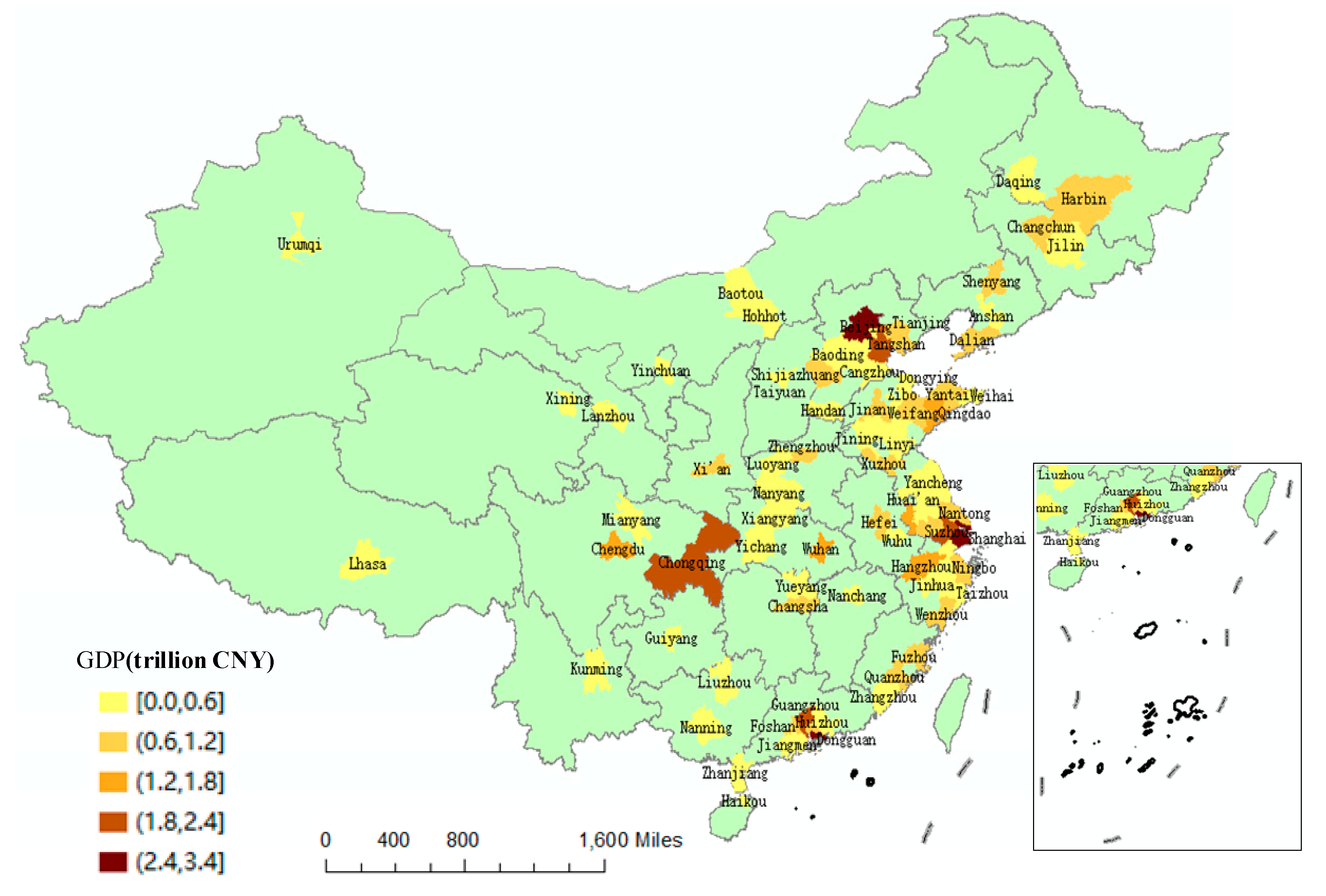
2.1. Study Areas
2.2. Data Collection
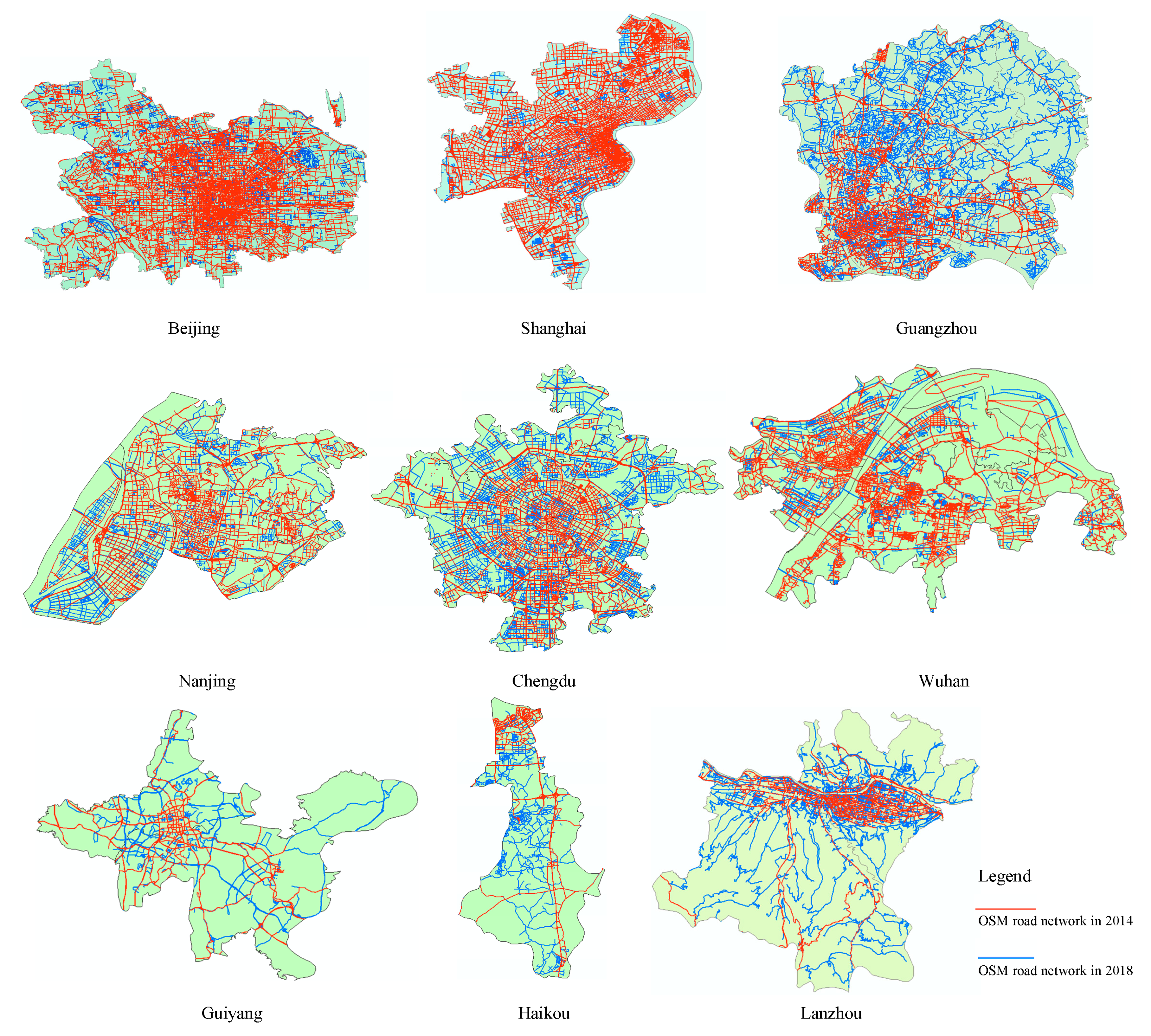
2.2.1. OSM Road Network
2.2.2. Municipal Gross Domestic Product
2.2.3. Exploring the Urban Area of Each Selected City
3. Methodology
Calculating the OSM Road Network Density of a City
4. Results and Analysis
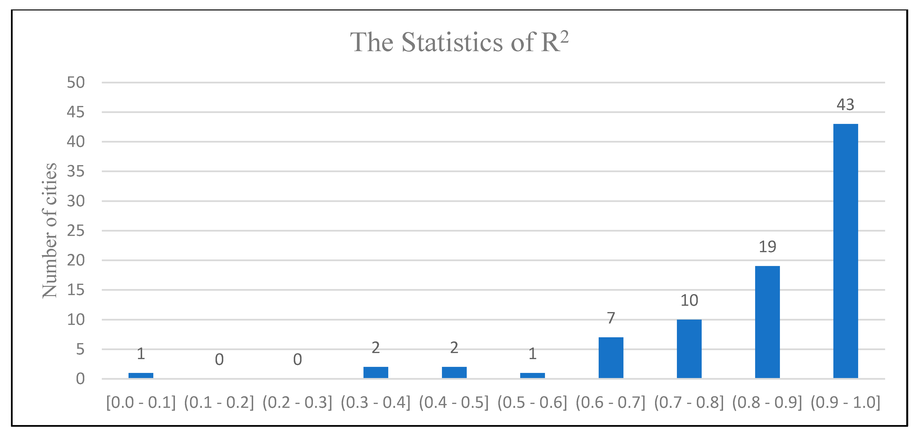
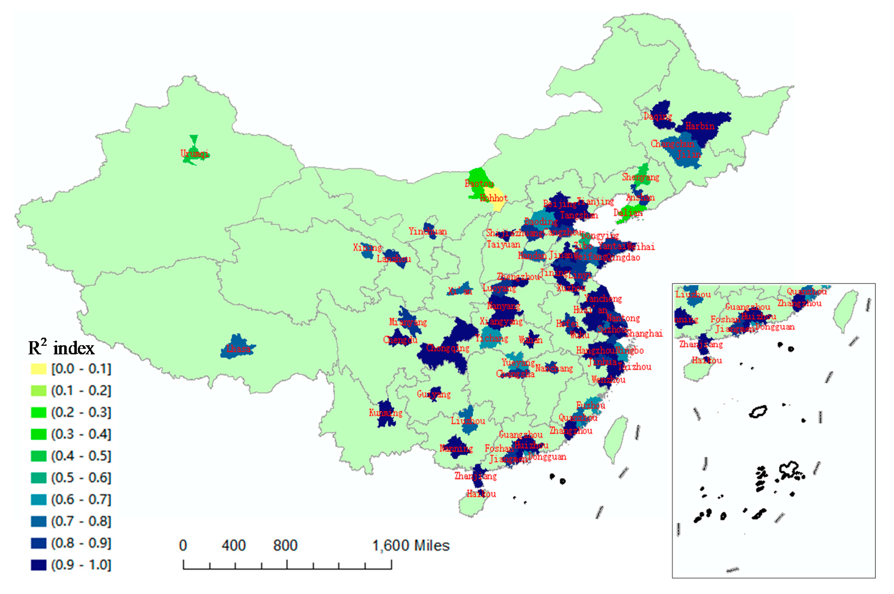
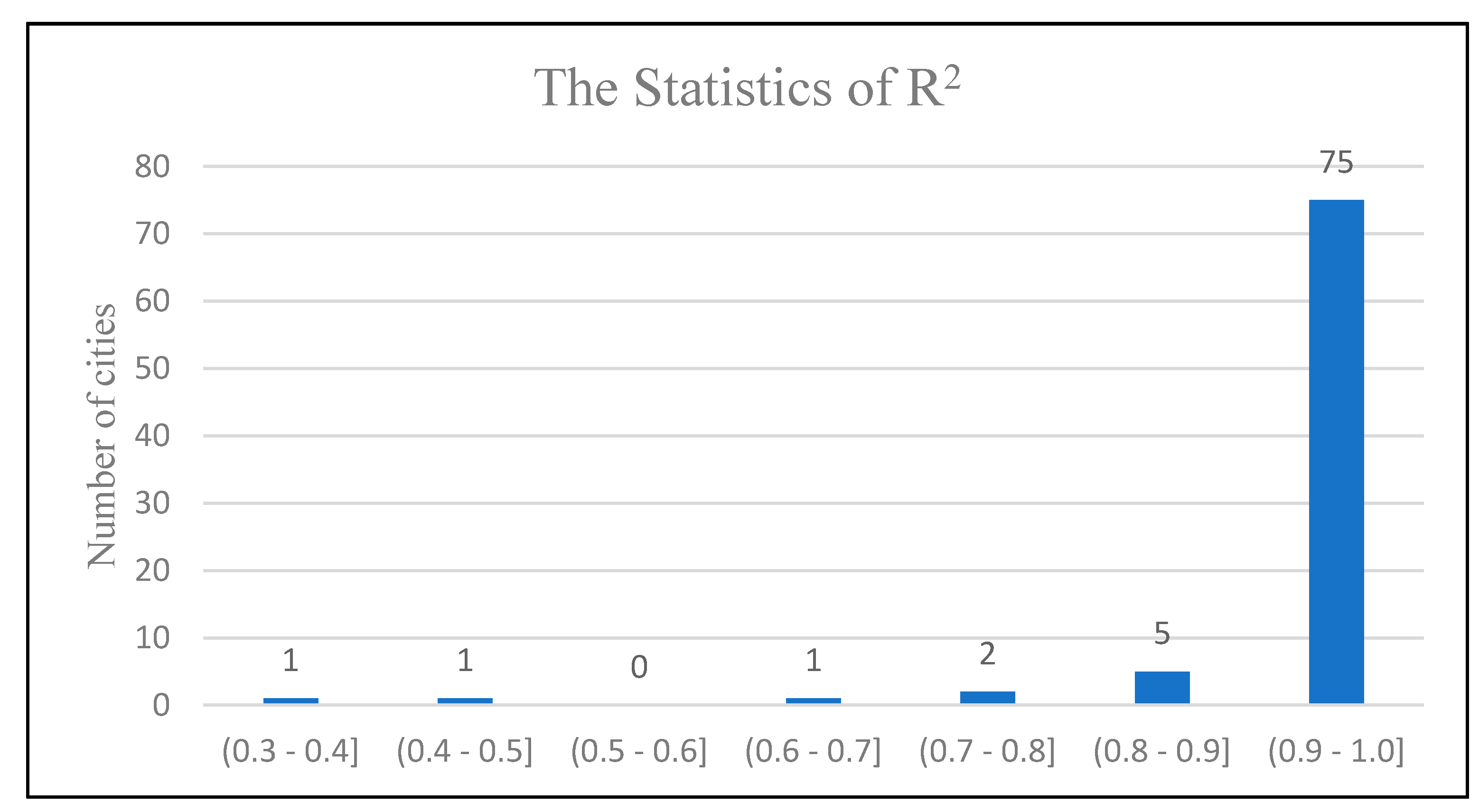
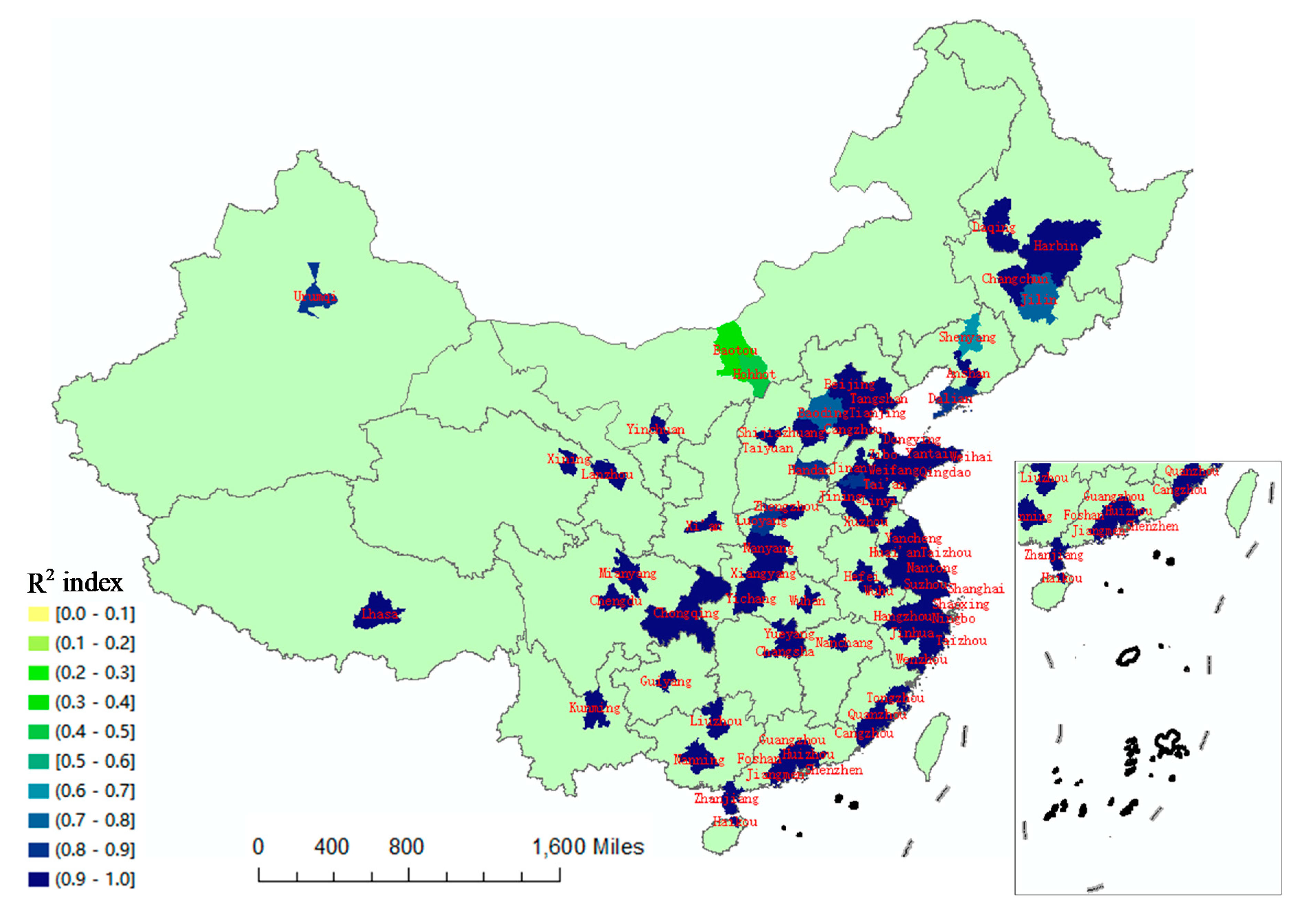
4.1. Fit Analysis
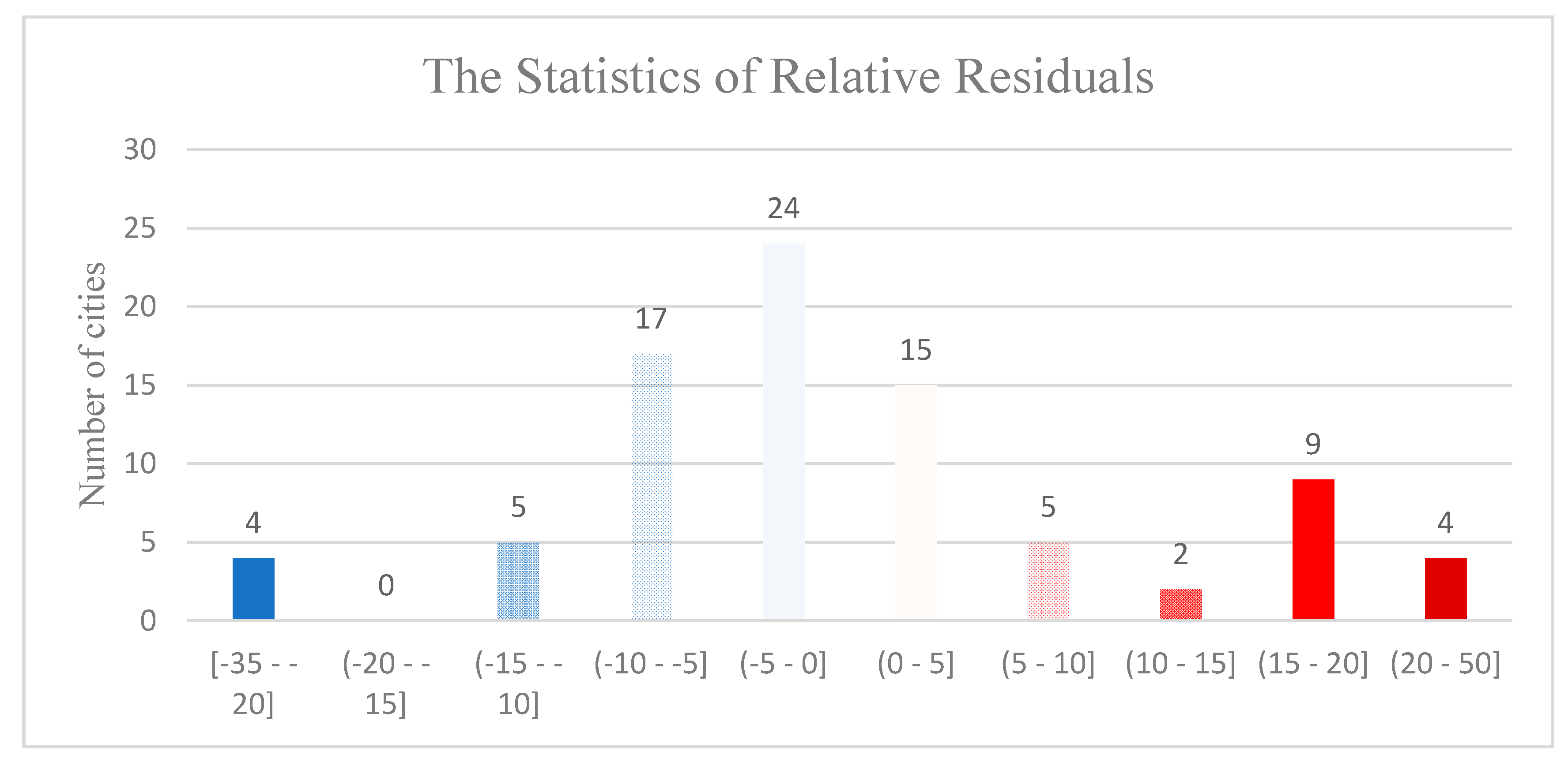
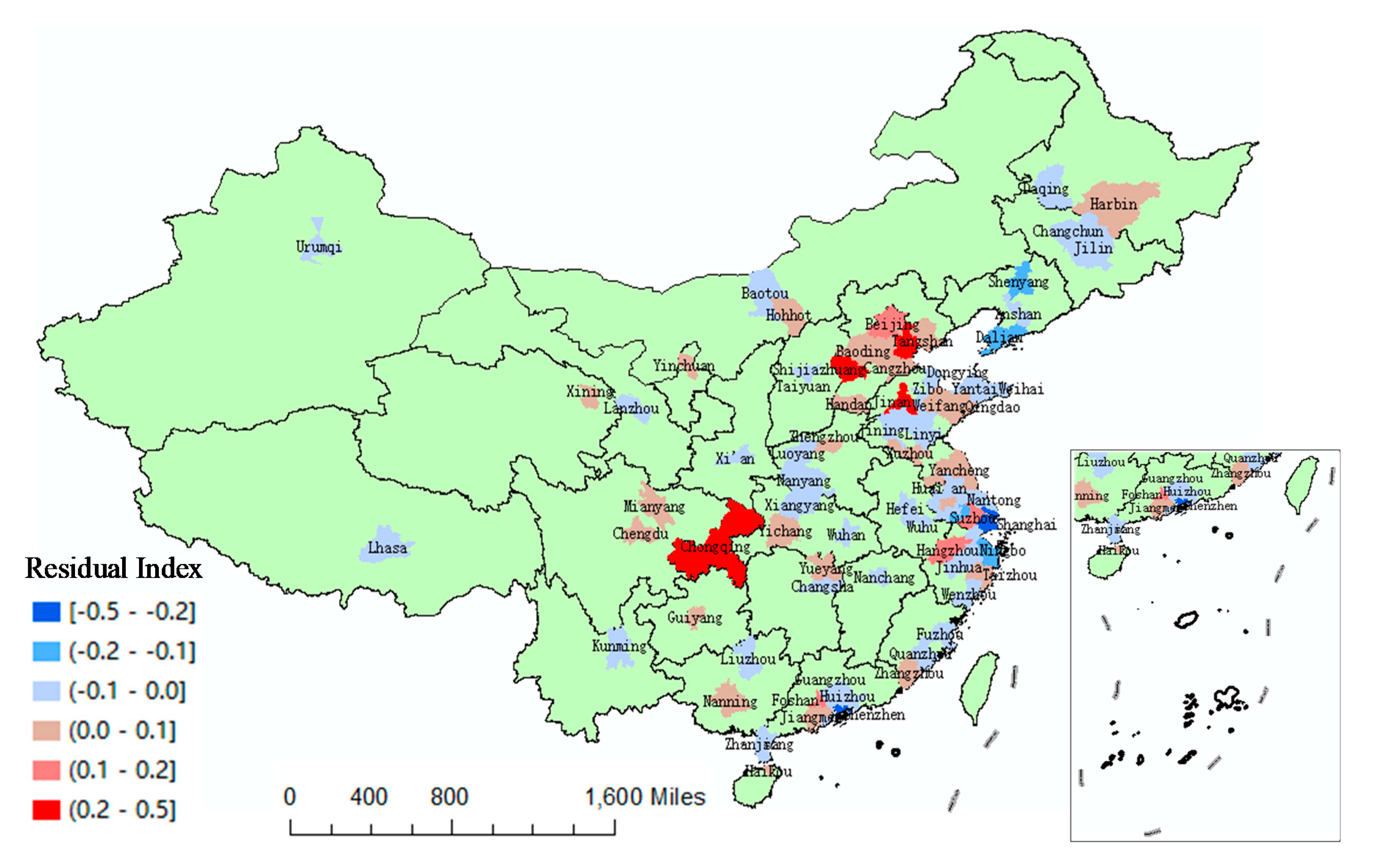
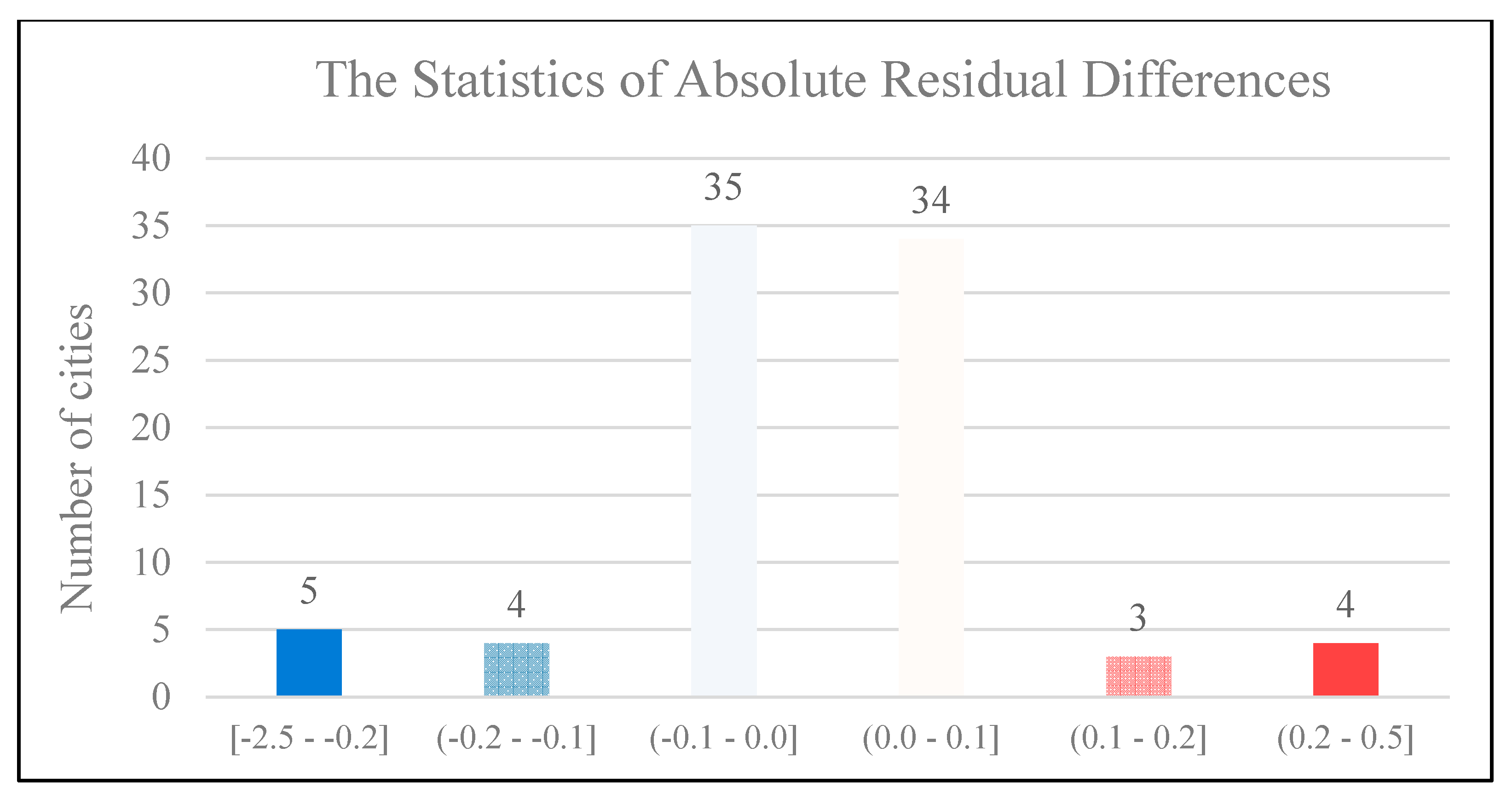
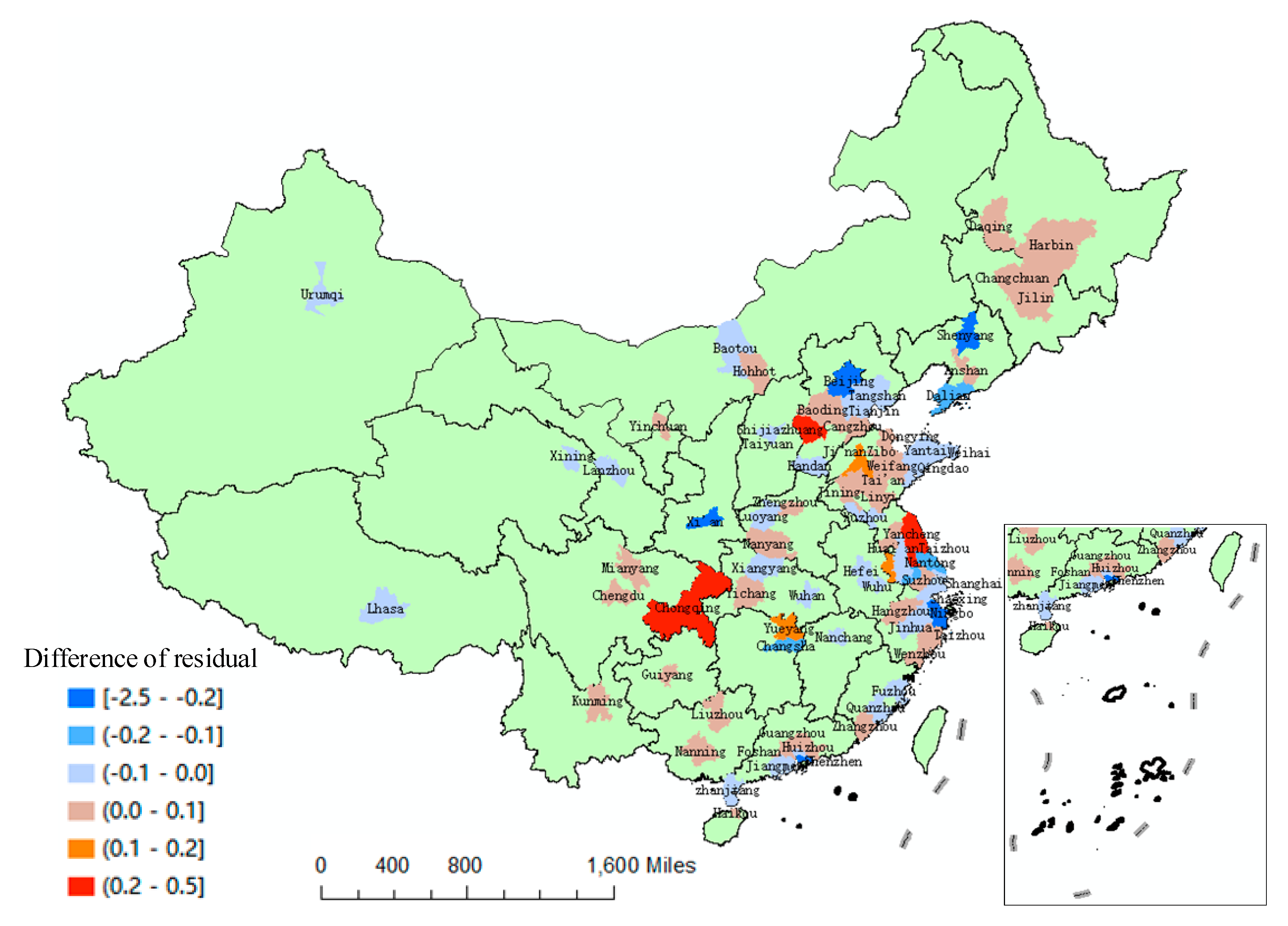
4.2. Validation of the Model
5. Conclusions
Author Contributions
Funding
Acknowledgments
Conflicts of Interest
Appendix A

| No. | Cities | Location of the Cities | Municipal GDP (trillion CNY) | OSM RND Represent the OSM Road Network Density | Regression Equation | Coefficient of Determination (R2) | ||||||
|---|---|---|---|---|---|---|---|---|---|---|---|---|
| 2014 | 2015 | 2016 | 2017 | 2014 | 2015 | 2016 | 2017 | |||||
| 1 | Beijing | Eastern | 2.13308 | 2.29686 | 2.48993 | 2.80004 | 4.958224 | 5.141546 | 5.357883 | 5.499061 | y = 1.174x − 3.721 | 0.9515 |
| 2 | Shanghai | Eastern | 2.356094 | 2.496499 | 2.746615 | 3.013386 | 3.155228 | 3.566878 | 4.213839 | 4.775253 | y = 0.4047x + 1.0635 | 0.9954 |
| 3 | Guangzhou | Eastern | 1.670687 | 1.810041 | 1.954744 | 2.150315 | 2.676991 | 3.534283 | 4.42808 | 5.49531 | y = 0.1697x + 1.212 | 0.999 |
| 4 | Shenzhen | Eastern | 1.600182 | 1.750286 | 1.94926 | 2.249006 | 6.827965 | 8.959036 | 9.394507 | 9.633126 | y = 0.1792x + 0.3274 | 0.6705 |
| 5 | Tianjin | Eastern | 1.572693 | 1.653819 | 1.788539 | 1.854919 | 5.901592 | 6.248347 | 6.441155 | 6.67073 | y = 0.3837x − 0.706 | 0.956 |
| 6 | Chongqing | Central | 1.42622 | 1.571727 | 1.774059 | 1.942473 | 0.662438 | 0.81481 | 0.900102 | 1.039407 | y = 1.4165x + 0.4687 | 0.9746 |
| 7 | Hangzhou | Eastern | 0.920616 | 1.005021 | 1.131372 | 1.260336 | 2.782885 | 3.022515 | 3.985984 | 4.35391 | y = 0.1934x + 0.3956 | 0.9616 |
| 8 | Nanjing | Eastern | 0.882075 | 0.972077 | 1.050302 | 1.17151 | 2.497384 | 2.930633 | 3.550194 | 4.445725 | y = 0.1445x + 0.5339 | 0.9909 |
| 9 | Qingdao | Eastern | 0.86921 | 0.930007 | 1.001129 | 1.103728 | 1.760078 | 1.887759 | 2.111393 | 2.364463 | y = 0.3787x + 0.2068 | 0.9962 |
| 10 | Dalian | Eastern | 0.765558 | 0.773164 | 0.68102 | 0.73639 | 1.75048 | 1.837818 | 1.917477 | 1.981108 | y = −0.2446x + 1.1969 | 0.3415 |
| 11 | Ningbo | Eastern | 0.761028 | 0.800361 | 0.868649 | 0.98421 | 1.560726 | 1.969064 | 2.056487 | 2.125499 | y = 0.31x + 0.256 | 0.6433 |
| 12 | Xiamen | Eastern | 0.327358 | 0.346603 | 0.378427 | 0.43517 | 6.883743 | 7.503913 | 7.690256 | 7.821306 | y = 0.0947x − 0.3358 | 0.6945 |
| 13 | Ji’nan | Eastern | 0.57706 | 0.610023 | 0.653612 | 0.720196 | 1.30219 | 1.353739 | 1.427773 | 1.692866 | y = 0.3468x + 0.1394 | 0.9479 |
| 14 | Suzhou | Eastern | 1.376089 | 1.450407 | 1.54751 | 1.731951 | 3.440061 | 3.859497 | 4.561366 | 6.548412 | y = 0.1107x + 1.0168 | 0.9822 |
| 15 | Wuhan | Central | 1.006948 | 1.09056 | 1.191261 | 1.341034 | 2.750418 | 2.951396 | 3.20614 | 3.695856 | y = 0.3509x + 0.0517 | 0.9939 |
| 16 | Chengdu | Western | 1.005683 | 1.080116 | 1.217023 | 1.388939 | 3.358756 | 4.236498 | 4.594147 | 5.561516 | y = 0.1801x + 0.3738 | 0.9487 |
| 17 | Changsha | Central | 0.782481 | 0.851013 | 0.945536 | 1.021013 | 1.533576 | 1.756367 | 2.052184 | 3.297249 | y = 0.1215x + 0.6375 | 0.8346 |
| 18 | Xi’an | Western | 0.549264 | 0.58012 | 0.625718 | 0.746985 | 3.196316 | 3.865494 | 4.135966 | 4.471107 | y = 0.1421x + 0.0688 | 0.7828 |
| 19 | Shenyang | Eastern | 0.709871 | 0.728 | 0.546001 | 0.586497 | 2.014167 | 2.150415 | 2.203039 | 2.292415 | y = −0.5466x + 1.8259 | 0.4997 |
| 20 | Zhengzhou | Eastern | 0.667699 | 0.731152 | 0.802531 | 0.91302 | 1.740456 | 2.115113 | 2.676731 | 2.880727 | y = 0.1937x + 0.3227 | 0.9216 |
| 21 | Dongguan | Eastern | 0.588118 | 0.627506 | 0.682767 | 0.758209 | 1.030598 | 1.501366 | 2.197582 | 2.854381 | y = 0.092x + 0.4898 | 0.992 |
| 22 | Fuzhou | Eastern | 0.516916 | 0.561808 | 0.619764 | 0.71034 | 0.902237 | 2.082021 | 2.257173 | 2.395907 | y = 0.0982x + 0.4147 | 0.6464 |
| 23 | Wuxi | Eastern | 0.820531 | 0.851826 | 0.921002 | 1.05118 | 2.153178 | 3.162821 | 3.301254 | 3.867276 | y = 0.1253x + 0.5199 | 0.7635 |
| 24 | Harbin | Eastern | 0.534007 | 0.575121 | 0.610161 | 0.635505 | 0.483118 | 0.51934 | 0.584794 | 0.615797 | y = 0.7215x + 0.1913 | 0.9782 |
| 25 | Foshan | Eastern | 0.760328 | 0.800392 | 0.863 | 0.95496 | 4.658889 | 5.297152 | 5.517081 | 5.916113 | y = 0.1522x + 0.0309 | 0.8897 |
| 26 | Changchun | Eastern | 0.534243 | 0.553003 | 0.591794 | 0.653003 | 0.937574 | 1.229054 | 1.432111 | 1.486014 | y = 0.1836x + 0.3497 | 0.7557 |
| 27 | Shijiazhuang | Eastern | 0.517027 | 0.54406 | 0.592773 | 0.646088 | 2.650926 | 2.756092 | 2.828802 | 2.846626 | y = 0.5834x − 1.0413 | 0.8326 |
| 28 | Taiyuan | Central | 0.253109 | 0.273534 | 0.29556 | 0.338218 | 0.925942 | 0.96981 | 1.230886 | 1.398845 | y = 0.1582x + 0.1111 | 0.9397 |
| 29 | Yantai | Eastern | 0.600208 | 0.644608 | 0.69257 | 0.733895 | 0.571782 | 0.624688 | 0.692235 | 0.923017 | y = 0.3473x + 0.4237 | 0.8592 |
| 30 | Hefei | Central | 0.515797 | 0.566027 | 0.627438 | 0.721345 | 1.07847 | 1.916291 | 2.42456 | 2.662393 | y = 0.1166x + 0.372 | 0.8532 |
| 31 | Kunming | Western | 0.371299 | 0.396801 | 0.430008 | 0.485764 | 0.764001 | 0.918156 | 1.01496 | 1.177625 | y = 0.2808x + 0.1489 | 0.9709 |
| 32 | Wenzhou | Eastern | 0.430281 | 0.461984 | 0.50454 | 0.545317 | 0.987931 | 1.447027 | 1.584584 | 2.000244 | y = 0.1169x + 0.3096 | 0.9462 |
| 33 | Nanning | Western | 0.31483 | 0.341009 | 0.370339 | 0.411883 | 0.304956 | 0.405285 | 0.406003 | 0.589919 | y = 0.3344x + 0.2169 | 0.9107 |
| 34 | Nanchang | Central | 0.366796 | 0.400001 | 0.435499 | 0.500319 | 4.445648 | 5.080118 | 5.207499 | 5.528507 | y = 0.1164x − 0.1642 | 0.8569 |
| 35 | Tangshan | Eastern | 0.62253 | 0.61 | 0.63062 | 0.71061 | 0.692859 | 0.858997 | 0.905533 | 1.472886 | y = 0.1277x + 0.518 | 0.9037 |
| 36 | Zibo | Eastern | 0.402977 | 0.41302 | 0.441201 | 0.478132 | 0.953503 | 0.988958 | 1.8103 | 2.013233 | y = 0.058x + 0.3503 | 0.8951 |
| 37 | Changzhou | Eastern | 0.490187 | 0.52732 | 0.577386 | 0.662228 | 1.340996 | 1.801608 | 1.848598 | 3.019328 | y = 0.1003x + 0.3634 | 0.9294 |
| 38 | Quanzhou | Eastern | 0.573336 | 0.613774 | 0.664663 | 0.754801 | 0.634438 | 0.920326 | 1.384851 | 1.342822 | y = 0.1867x + 0.4517 | 0.7318 |
| 39 | Guiyang | Eastern | 0.249727 | 0.289116 | 0.31577 | 0.353796 | 1.4045 | 1.561081 | 1.73026 | 2.215922 | y = 0.1197x + 0.0952 | 0.9203 |
| 40 | Jiaxing | Eastern | 0.33528 | 0.351706 | 0.37601 | 0.435524 | 1.127291 | 1.266025 | 1.598774 | 1.725241 | y = 0.1447x + 0.1678 | 0.8476 |
| 41 | Nantong | Eastern | 0.565279 | 0.61484 | 0.67682 | 0.77346 | 0.587234 | 1.243394 | 2.189651 | 2.424369 | y = 0.0989x + 0.4982 | 0.8832 |
| 42 | Jinhua | Eastern | 0.320664 | 0.34065 | 0.363501 | 0.387022 | 0.314445 | 0.663407 | 0.705874 | 0.910499 | y = 0.1096x + 0.2819 | 0.8947 |
| 43 | Zhuhai | Eastern | 0.185732 | 0.202498 | 0.222637 | 0.256473 | 2.257383 | 2.892806 | 3.178339 | 3.573405 | y = 0.0525x + 0.0605 | 0.9154 |
| 44 | Huizhou | Eastern | 0.30007 | 0.314003 | 0.341217 | 0.383058 | 0.54594 | 0.681892 | 0.733018 | 0.937024 | y = 0.2204x + 0.1749 | 0.9566 |
| 45 | Xuzhou | Eastern | 0.496391 | 0.531988 | 0.580852 | 0.660595 | 0.839667 | 0.833549 | 1.604102 | 3.131913 | y = 0.0638x + 0.4653 | 0.9418 |
| 46 | Haikou | Eastern | 0.10917 | 0.116196 | 0.125767 | 0.139058 | 1.215575 | 1.39047 | 1.391586 | 1.593147 | y = 0.0796x + 0.0113 | 0.9019 |
| 47 | Urumqi | Western | 0.246147 | 0.263164 | 0.245898 | 0.274382 | 1.471562 | 1.488615 | 1.548517 | 1.676137 | y = 0.1043x + 0.0962 | 0.4828 |
| 48 | Shaoxing | Eastern | 0.426583 | 0.446665 | 0.471 | 0.510804 | 0.758167 | 0.803163 | 1.000226 | 1.245672 | y = 0.1613x + 0.3103 | 0.9789 |
| 49 | Zhongshan | Eastern | 0.28233 | 0.301003 | 0.320278 | 0.345031 | 1.636848 | 1.759837 | 2.144733 | 2.393204 | y = 0.0758x + 0.1617 | 0.9693 |
| 50 | Taizhou (Zhejiang) | Eastern | 0.338751 | 0.355813 | 0.384281 | 0.438822 | 0.531115 | 0.576276 | 0.832387 | 1.119472 | y = 0.1603x + 0.2568 | 0.9833 |
| 51 | Lanzhou | Western | 0.200094 | 0.209599 | 0.226423 | 0.252354 | 0.623852 | 0.644902 | 0.723011 | 1.678987 | y = 0.0412x + 0.1843 | 0.8392 |
| 52 | Weifang | Eastern | 0.478674 | 0.517053 | 0.55227 | 0.585863 | 0.808287 | 1.067039 | 1.251496 | 2.839208 | y = 0.0438x + 0.4681 | 0.7604 |
| 53 | Baoding | Eastern | 0.30352 | 0.300034 | 0.32273 | 0.35809 | 1.08439 | 1.307091 | 1.321359 | 1.482171 | y = 0.1299x + 0.1524 | 0.637 |
| 54 | Zhenjiang | Eastern | 0.325238 | 0.350248 | 0.383384 | 0.401036 | 0.877717 | 1.211188 | 1.385888 | 1.712882 | y = 0.0949x + 0.2419 | 0.955 |
| 55 | Yangzhou | Eastern | 0.369789 | 0.401684 | 0.444938 | 0.506492 | 1.440231 | 1.801123 | 2.298118 | 2.526604 | y = 0.117x + 0.1947 | 0.9365 |
| 56 | Hohhot | Western | 0.289405 | 0.309052 | 0.317359 | 0.274372 | 0.567368 | 0.655892 | 0.859838 | 0.869946 | y = −0.0029x + 0.2997 | 0.0005 |
| 57 | Langfang | Eastern | 0.217596 | 0.24019 | 0.27063 | 0.28806 | 0.437621 | 0.726791 | 0.791253 | 1.032201 | y = 0.1226x + 0.1626 | 0.9129 |
| 58 | Luoyang | Central | 0.328457 | 0.350875 | 0.37829 | 0.429019 | 0.908334 | 1.110387 | 1.912928 | 2.084188 | y = 0.069x + 0.2679 | 0.856 |
| 59 | Weihai | Eastern | 0.279034 | 0.300157 | 0.32122 | 0.34801 | 1.158146 | 1.249603 | 1.297057 | 1.523613 | y = 0.1835x + 0.0723 | 0.935 |
| 60 | Yancheng | Eastern | 0.383562 | 0.42125 | 0.457608 | 0.508269 | 0.657349 | 0.692985 | 0.894144 | 1.233145 | y = 0.194x + 0.274 | 0.9275 |
| 61 | Linyi | Eastern | 0.35698 | 0.37632 | 0.402675 | 0.434539 | 1.480754 | 2.084111 | 2.317847 | 2.54728 | y = 0.0686x + 0.2481 | 0.8741 |
| 62 | Jiangmen | Eastern | 0.208276 | 0.224002 | 0.241878 | 0.269025 | 1.3465 | 1.558839 | 1.660016 | 1.74101 | y = 0.1434x + 0.0097 | 0.8806 |
| 63 | Taizhou (Jiangsu) | Eastern | 0.337089 | 0.365553 | 0.410178 | 0.474453 | 0.822494 | 1.257907 | 1.596425 | 2.136174 | y = 0.107x + 0.2414 | 0.9821 |
| 64 | Zhangzhou | Eastern | 0.250636 | 0.276745 | 0.312534 | 0.352853 | 0.916913 | 1.151741 | 1.200081 | 1.38604 | y = 0.2206x + 0.0414 | 0.9201 |
| 65 | Handan | Eastern | 0.308001 | 0.31454 | 0.33371 | 0.36663 | 0.675282 | 0.813087 | 0.914555 | 0.949443 | y = 0.1836x + 0.1769 | 0.7366 |
| 66 | Jining | Western | 0.380006 | 0.401312 | 0.430182 | 0.465057 | 0.471934 | 0.526896 | 0.776055 | 0.91366 | y = 0.1739x + 0.3022 | 0.966 |
| 67 | Wuhu | Eastern | 0.23079 | 0.245732 | 0.269944 | 0.306552 | 0.672768 | 0.965252 | 1.227687 | 1.957186 | y = 0.0598x + 0.1912 | 0.9873 |
| 68 | Yinchuan | Central | 0.139567 | 0.148073 | 0.161728 | 0.180317 | 0.497675 | 0.59603 | 0.693312 | 0.716513 | y = 0.164x + 0.0548 | 0.8525 |
| 69 | Liuzhou | Eastern | 0.220851 | 0.229862 | 0.247694 | 0.275564 | 0.455206 | 0.485649 | 0.604588 | 0.599445 | y = 0.2719x + 0.0977 | 0.7542 |
| 70 | Mianyang | Western | 0.157989 | 0.170033 | 0.183042 | 0.207475 | 0.445944 | 0.554054 | 0.707322 | 0.734055 | y = 0.1434x + 0.0921 | 0.838 |
| 71 | Zhanjiang | Eastern | 0.22587 | 0.238002 | 0.258478 | 0.282403 | 1.405769 | 1.659609 | 2.261492 | 2.575143 | y = 0.0455x + 0.1613 | 0.9729 |
| 72 | Anshan | Eastern | 0.2349 | 0.2326 | 0.14408 | 0.16021 | 0.727266 | 0.768087 | 0.816542 | 0.828872 | y = −0.9284x + 0.9219 | 0.8297 |
| 73 | Daqing | Eastern | 0.407 | 0.29835 | 0.261 | 0.26805 | 0.499983 | 1.191177 | 1.2228 | 1.222723 | y = −0.1858x + 0.5007 | 0.9601 |
| 74 | Yichang | Central | 0.313221 | 0.33848 | 0.370936 | 0.385717 | 1.996736 | 2.126815 | 2.172778 | 2.900025 | y = 0.0641x + 0.2048 | 0.6429 |
| 75 | Baotou | Eastern | 0.363631 | 0.378193 | 0.386763 | 0.275303 | 0.601152 | 0.628997 | 0.851639 | 0.900335 | y = −0.1854x + 0.4892 | 0.3029 |
| 76 | Jilin | Eastern | 0.27302 | 0.24552 | 0.253135 | 0.23028 | 0.601762 | 0.695863 | 0.781348 | 0.880384 | y = −0.1324x + 0.3484 | 0.7854 |
| 77 | Huai’an | Eastern | 0.245539 | 0.274509 | 0.3048 | 0.338743 | 0.549558 | 0.656979 | 0.695744 | 0.776926 | y = 0.4165x + 0.0119 | 0.9658 |
| 78 | Cangzhou | Eastern | 0.313338 | 0.32406 | 0.35334 | 0.38169 | 0.746255 | 0.809976 | 0.888409 | 1.36473 | y = 0.1017x + 0.2462 | 0.8629 |
| 79 | Xiangyang | Central | 0.31293 | 0.338212 | 0.369451 | 0.40649 | 0.347927 | 0.424744 | 0.563634 | 0.594033 | y = 0.3347x + 0.1952 | 0.9255 |
| 80 | Yueyang | Central | 0.266939 | 0.288628 | 0.310087 | 0.325803 | 0.78718 | 0.829211 | 0.870221 | 1.291411 | y = 0.0898x + 0.2131 | 0.67 |
| 81 | Taian | Eastern | 0.300219 | 0.31584 | 0.33168 | 0.358528 | 0.935667 | 1.041736 | 1.769295 | 1.918874 | y = 0.0462x + 0.2612 | 0.8588 |
| 82 | Dongying | Eastern | 0.343049 | 0.345064 | 0.34796 | 0.380178 | 0.455815 | 0.496966 | 0.737227 | 0.774951 | y = 0.0783x + 0.3058 | 0.5307 |
| 83 | Nanyang | Central | 0.267688 | 0.287502 | 0.311877 | 0.33777 | 0.32572 | 0.387065 | 0.39798 | 0.513531 | y = 0.3688x + 0.1515 | 0.9074 |
| 84 | Xining | Western | 0.106578 | 0.113162 | 0.124817 | 0.12849 | 2.148855 | 2.336419 | 2.553052 | 2.433314 | y = 0.0526x − 0.0062 | 0.7804 |
| 85 | Lhasa | Western | 0.034745 | 0.038946 | 0.042495 | 0.047916 | 0.497234 | 0.788384 | 0.857679 | 0.901169 | y = 0.0273x + 0.0203 | 0.7902 |
| No. | Cities | Location of the Cities | GDP in 2018 (trillion CNY) | Predictive GDP in 2018 by Using OSM Road Network Density (trillion CNY) | Predictive GDP in 2018 by Using OSM Road Network Density and Population (trillion CNY) | Absolute Residuals by Using OSM Road Network Density | Relative Residuals by Using OSM Road Network Density | Absolute Residuals by Using OSM Road Network Density and Population | Relative Residuals by Using OSM Road Network Density and Population |
|---|---|---|---|---|---|---|---|---|---|
| 1 | Beijing | Eastern | 3.0320 | 3.1938 | 3.4422 | 0.1618 | 5.3364 | 0.4102 | 13.5290 |
| 2 | Shanghai | Eastern | 3.2680 | 3.0637 | 3.0811 | −0.2043 | −6.2515 | −0.1869 | −5.7191 |
| 3 | Guangzhou | Eastern | 2.2859 | 2.2386 | 2.2264 | −0.0473 | −2.0692 | −0.0595 | −2.6029 |
| 4 | Shenzhen | Eastern | 2.4222 | 2.1405 | 2.4473 | −0.2817 | −11.6299 | 0.0251 | 1.0362 |
| 5 | Tianjin | Eastern | 1.8810 | 2.1958 | 2.2128 | 0.3149 | 16.7358 | 0.3318 | 17.6396 |
| 6 | Chongqing | Central | 2.0363 | 2.4803 | 2.0682 | 0.4440 | 21.8043 | 0.0319 | 1.5666 |
| 7 | Hangzhou | Eastern | 1.3509 | 1.5446 | 1.5063 | 0.1937 | 14.3386 | 0.1554 | 11.5034 |
| 8 | Nanjing | Eastern | 1.2820 | 1.2024 | 1.0471 | −0.0797 | −6.2090 | −0.2349 | −18.3229 |
| 9 | Qingdao | Eastern | 1.2002 | 1.2330 | 1.2537 | 0.0328 | 2.7329 | 0.0535 | 4.4576 |
| 10 | Dalian | Eastern | 0.7669 | 0.5997 | 0.7002 | −0.1672 | −21.8021 | −0.0667 | −8.6974 |
| 11 | Ningbo | Eastern | 1.0746 | 0.9531 | 1.1785 | −0.1215 | −11.3065 | 0.1039 | 9.6687 |
| 12 | Xiamen | Eastern | 0.4791 | 0.4474 | 0.4887 | −0.0317 | −6.6166 | 0.0096 | 2.0038 |
| 13 | Ji’nan | Eastern | 0.7857 | 1.0287 | 0.8826 | 0.2430 | 30.9278 | 0.0969 | 12.3330 |
| 14 | Suzhou | Eastern | 1.8565 | 1.9590 | 1.9216 | 0.1025 | 5.5211 | 0.0651 | 3.5066 |
| 15 | Wuhan | Central | 1.4847 | 1.4228 | 1.4250 | −0.0619 | −4.1692 | −0.0597 | −4.0210 |
| 16 | Chengdu | Western | 1.5254 | 1.5929 | 1.5392 | 0.0675 | 4.4251 | 0.0138 | 0.9047 |
| 17 | Changsha | Central | 1.1003 | 1.0682 | 1.2354 | −0.0322 | −2.9174 | 0.1351 | 12.2785 |
| 18 | Xi’an | Western | 0.8350 | 0.7505 | 1.2377 | −0.0845 | −10.1198 | 0.4027 | 48.2275 |
| 19 | Shenyang | Eastern | 0.6292 | 0.4871 | 2.5457 | −0.1421 | −22.5842 | 1.9165 | 304.5931 |
| 20 | Zhengzhou | Eastern | 1.0143 | 1.0272 | 1.0107 | 0.0128 | 1.2718 | −0.0036 | −0.3549 |
| 21 | Dongguan | Eastern | 0.8279 | 0.8223 | 0.8294 | −0.0056 | −0.6764 | 0.0015 | 0.1812 |
| 22 | Fuzhou | Eastern | 0.7857 | 0.6961 | 0.7764 | −0.0895 | −11.4038 | −0.0093 | −1.1837 |
| 23 | Wuxi | Eastern | 1.1439 | 1.0292 | 1.1492 | −0.1146 | −10.0271 | 0.0053 | 0.4633 |
| 24 | Harbin | Eastern | 0.6301 | 0.6759 | 0.6757 | 0.0458 | 7.2687 | 0.0456 | 7.2369 |
| 25 | Foshan | Eastern | 0.9936 | 1.1602 | 1.1390 | 0.1666 | 16.7673 | 0.1454 | 14.6337 |
| 26 | Changchun | Eastern | 0.7176 | 0.6533 | 0.6331 | −0.0643 | −8.9604 | −0.0845 | −11.7754 |
| 27 | Shijiazhuang | Eastern | 0.6083 | 0.8995 | 0.5967 | 0.2913 | 47.8711 | −0.0116 | −1.9070 |
| 28 | Taiyuan | Central | 0.3884 | 0.3584 | 0.3837 | −0.0301 | −7.7240 | −0.0047 | −1.2101 |
| 29 | Yantai | Eastern | 0.7833 | 0.7658 | 0.7777 | −0.0174 | −2.2341 | −0.0056 | −0.7149 |
| 30 | Hefei | Central | 0.7823 | 0.7452 | 0.8277 | −0.0371 | −4.7424 | 0.0454 | 5.8034 |
| 31 | Kunming | Western | 0.5207 | 0.5186 | 0.4968 | −0.0021 | −0.4033 | −0.0239 | −4.5900 |
| 32 | Wenzhou | Eastern | 0.6006 | 0.5519 | 0.5490 | −0.0487 | −8.1086 | −0.0516 | −8.5914 |
| 33 | Nanning | Western | 0.4147 | 0.4548 | 0.4532 | 0.0401 | 9.6696 | 0.0385 | 9.2838 |
| 34 | Nanchang | Central | 0.5275 | 0.5144 | 0.5443 | −0.0131 | −2.4834 | 0.0168 | 3.1848 |
| 35 | Tangshan | Eastern | 0.6955 | 0.7423 | 0.7444 | 0.0468 | 6.7290 | 0.0489 | 7.0309 |
| 36 | Zibo | Eastern | 0.5068 | 0.4839 | 0.4693 | −0.0230 | −4.5185 | −0.0375 | −7.3994 |
| 37 | Changzhou | Eastern | 0.7050 | 0.6780 | 0.7372 | −0.0270 | −3.8298 | 0.0322 | 4.5674 |
| 38 | Quanzhou | Eastern | 0.8468 | 0.7687 | 0.7780 | −0.0781 | −9.2230 | −0.0688 | −8.1247 |
| 39 | Guiyang | Eastern | 0.3798 | 0.4347 | 0.3671 | 0.0549 | 14.4550 | −0.0127 | −3.3439 |
| 40 | Jiaxing | Eastern | 0.4872 | 0.4513 | 0.4875 | −0.0359 | −7.3686 | 0.0003 | 0.0616 |
| 41 | Nantong | Eastern | 0.8427 | 0.7887 | 0.9330 | −0.0540 | −6.4080 | 0.0903 | 10.7156 |
| 42 | Jinhua | Eastern | 0.4100 | 0.3952 | 0.4049 | −0.0148 | −3.6098 | −0.0051 | −1.2439 |
| 43 | Zhuhai | Eastern | 0.2915 | 0.2626 | 0.3010 | −0.0288 | −9.9142 | 0.0095 | 3.2590 |
| 44 | Huizhou | Eastern | 0.4103 | 0.3910 | 0.3898 | −0.0193 | −4.7039 | −0.0205 | −4.9963 |
| 45 | Xuzhou | Eastern | 0.6755 | 0.6919 | 0.7017 | 0.0164 | 2.4278 | 0.0262 | 3.8786 |
| 46 | Haikou | Eastern | 0.1511 | 0.2083 | 0.1459 | 0.0573 | 37.8557 | −0.0052 | −3.4414 |
| 47 | Urumqi | Western | 0.3100 | 0.2892 | 0.3181 | −0.0207 | −6.7097 | 0.0081 | 2.6129 |
| 48 | Shaoxing | Eastern | 0.5417 | 0.5172 | 0.5427 | −0.0244 | −4.5228 | 0.001 | 0.1846 |
| 49 | Zhongshan | Eastern | 0.3633 | 0.3738 | 0.4142 | 0.0105 | 2.8902 | 0.0509 | 14.0105 |
| 50 | Taizhou (Zhejiang) | Eastern | 0.4875 | 0.4979 | 0.4914 | 0.0105 | 2.1333 | 0.0039 | 0.8000 |
| 51 | Lanzhou | Western | 0.2733 | 0.2572 | 0.2673 | −0.0161 | −5.8910 | −0.006 | −2.1954 |
| 52 | Weifang | Eastern | 0.6157 | 0.6289 | 0.6077 | 0.0132 | 2.1439 | −0.008 | −1.2993 |
| 53 | Baoding | Eastern | 0.3590 | 0.4259 | 0.4253 | 0.0669 | 18.6351 | 0.0663 | 18.4680 |
| 54 | Zhenjiang | Eastern | 0.4050 | 0.4095 | 0.5013 | 0.0045 | 1.1111 | 0.0963 | 23.7778 |
| 55 | Yangzhou | Eastern | 0.5466 | 0.5026 | 0.5821 | −0.0440 | −8.0498 | 0.0355 | 6.4947 |
| 56 | Hohhot | Western | 0.2904 | 0.2969 | 0.2957 | 0.0066 | 2.2383 | 0.0053 | 1.8251 |
| 57 | Langfang | Eastern | 0.3108 | 0.3112 | 0.3174 | 0.0004 | 0.1287 | 0.0066 | 2.1236 |
| 58 | Luoyang | Central | 0.4641 | 0.4307 | 0.4405 | −0.0334 | −7.1967 | −0.0236 | −5.0851 |
| 59 | Weihai | Eastern | 0.3641 | 0.3568 | 0.3589 | −0.0073 | −2.0049 | −0.0052 | −1.4282 |
| 60 | Yancheng | Eastern | 0.5487 | 0.5544 | 0.3228 | 0.0057 | 1.0388 | −0.2259 | −41.1700 |
| 61 | Linyi | Eastern | 0.4718 | 0.4571 | 0.4416 | −0.0147 | −3.1157 | −0.0302 | −6.4010 |
| 62 | Jiangmen | Eastern | 0.2900 | 0.2910 | 0.3001 | 0.0010 | 0.3448 | 0.0101 | 3.4828 |
| 63 | Taizhou (Jiangsu) | Eastern | 0.5108 | 0.4790 | 0.2763 | −0.0317 | −6.2255 | −0.2345 | −45.9084 |
| 64 | Zhangzhou | Eastern | 0.3948 | 0.4722 | 0.4006 | 0.0774 | 19.6049 | 0.0058 | 1.4691 |
| 65 | Handan | Eastern | 0.3455 | 0.3577 | 0.3600 | 0.0122 | 3.5311 | 0.0145 | 4.1968 |
| 66 | Jining | Western | 0.4931 | 0.4905 | 0.4776 | −0.0026 | −0.5273 | −0.0155 | −3.1434 |
| 67 | Wuhu | Eastern | 0.3279 | 0.3260 | 0.3294 | −0.0019 | −0.5794 | 0.0015 | 0.4575 |
| 68 | Yinchuan | Central | 0.1901 | 0.2211 | 0.1720 | 0.0309 | 16.3072 | −0.0181 | −9.5213 |
| 69 | Liuzhou | Eastern | 0.3084 | 0.3025 | 0.2880 | −0.0059 | −1.9131 | −0.0204 | −6.6148 |
| 70 | Mianyang | Western | 0.2304 | 0.2376 | 0.1645 | 0.0072 | 3.1250 | −0.0659 | −28.6024 |
| 71 | Zhanjiang | Eastern | 0.3008 | 0.2947 | 0.2966 | −0.0061 | −2.0279 | −0.0042 | −1.3963 |
| 72 | Anshan | Eastern | 0.1751 | 0.1145 | 0.1012 | −0.0606 | −34.6088 | −0.0739 | −42.2045 |
| 73 | Daqing | Eastern | 0.2801 | 0.2620 | 0.2582 | −0.0181 | −6.4620 | −0.0219 | −7.8186 |
| 74 | Yichang | Central | 0.4064 | 0.4784 | 0.3904 | 0.0720 | 17.7165 | −0.016 | −3.9370 |
| 75 | Baotou | Eastern | 0.2952 | 0.2298 | 0.3095 | −0.0654 | −22.1545 | 0.0143 | 4.8442 |
| 76 | Jilin | Eastern | 0.2210 | 0.2180 | 0.2167 | −0.0030 | −1.3575 | −0.0043 | −1.9457 |
| 77 | Huai’an | Eastern | 0.3601 | 0.4267 | 0.3499 | 0.0666 | 18.4949 | −0.0102 | −2.8325 |
| 78 | Cangzhou | Eastern | 0.3676 | 0.4266 | 0.4065 | 0.0590 | 16.0501 | 0.0389 | 10.5822 |
| 79 | Xiangyang | Central | 0.4310 | 0.4096 | 0.4381 | −0.0214 | −4.9652 | 0.0071 | 1.6473 |
| 80 | Yueyang | Central | 0.3411 | 0.4007 | 0.3001 | 0.0596 | 17.4729 | −0.041 | −12.0199 |
| 81 | Taian | Eastern | 0.3652 | 0.3579 | 0.3465 | −0.0072 | −1.9989 | −0.0187 | −5.1205 |
| 82 | Dongying | Eastern | 0.4152 | 0.4105 | 0.3266 | −0.0047 | −1.1320 | −0.0886 | −21.3391 |
| 83 | Nanyang | Central | 0.3567 | 0.3501 | 0.3379 | −0.0066 | −1.8503 | −0.0188 | −5.2705 |
| 84 | Xining | Western | 0.1286 | 0.1322 | 0.1360 | 0.0035 | 2.7994 | 0.0074 | 5.7543 |
| 85 | Lhasa | Western | 0.0528 | 0.0486 | 0.0515 | −0.0042 | −7.9545 | −0.0013 | −2.4621 |
References
- Gustafson, E.J. Quantifying landscape spatial pattern: What is the state of the art? Ecosystems 1998, 1, 143–156. [Google Scholar] [CrossRef]
- Hargis, C.D.; Bissonette, J.A.; David, J.L. The behavior of landscape metrics commonly used in the study of habitat fragmentation. Landsc. Ecol. 1998, 13, 167–186. [Google Scholar] [CrossRef]
- O’Neill, R.V.; Krummel, J.R.; Gardner, R.H.; Sugihara, G.; Jackson, B.; DeAngelis, D.L.; Milne, B.T.; Turner, M.G.; Zygmunt, B.; Christensen, S.W.; et al. Indices of landscape pattern. Landsc. Ecol. 1988, 1, 153–162. [Google Scholar] [CrossRef]
- McGarigal, K.; Cushman, S.A.; Neel, M.C.; Ene, E. FRAGSTATS: Spatial Pattern Analysis Program for Categorical Maps. 2002. Available online: www.umass.edu/landeco/research/fragstats/fragstats.html (accessed on 15 May 2020).
- Herold, M.; Liu, X.H.; Clarke, K.C. Spatial Metrics and Image Texture for Mapping Urban Land use. Photogramm. Eng. Remote Sens. 2003, 69, 991–1001. [Google Scholar] [CrossRef] [Green Version]
- Herold, M.; Couclelis, H.; Clarke, K.C. The role of spatial metrics in the analysis and modeling of urban land use change. Comput. Environ. Urban Syst. 2005, 29, 369–399. [Google Scholar] [CrossRef]
- Reis, J.P.; Silva, E.A.; Pinbo, P. Measure space: A review of spatial metrics for urban growth and shrinkage. In The Routledge Handbook of Planning Research Methods; Silva, E.A., Healey, P., Harris, N., Van den Broeck, P., Eds.; Routledge: New York, NY, USA, 2014; pp. 279–292. [Google Scholar]
- Reis, J.P.; Silva, E.A.; Pinbo, P. Spatial metrics to study urban patterns in growing and shrinking cities. Urban Geogr. 2016, 37, 246–271. [Google Scholar] [CrossRef]
- Chen, M.; Huang, Y.; Tang, Z.; Lu, D.; Liu, H.; Ma, L. The provincial pattern of the relationship between urbanization and economic development in China. J. Geogr. Sci. 2014, 24, 33–45. [Google Scholar] [CrossRef]
- Henderson, V. The Urbanization Process and Economic Growth: The So-What Question. J. Econ. Growth 2003, 8, 47–71. [Google Scholar] [CrossRef]
- Njoh, A.J. Urbanization and development in sub-Saharan Africa. Cities 2003, 20, 167–174. [Google Scholar] [CrossRef]
- Liu, Y.S.; Fang, F.; Li, Y.H. Key issues of land use in China and implications for policy making. Land Use Policy 2014, 40, 6–12. [Google Scholar] [CrossRef]
- Xiang, W.N.; Stuber, R.M.B.; Meng, X.C. Meeting critical challengers and striving for urban sustainability in China. Landsc. Urban Plan. 2011, 100, 418–420. [Google Scholar] [CrossRef] [PubMed]
- Li, Y.Z. Urbanization and economic growth in China: An empirical research based on VAR model. Int. J. Econ. Financ. 2017, 9, 210–219. [Google Scholar]
- Cai, Z.Y.; Liu, Q.; Cao, S.X. Real estate supports rapid development of China’s urbanization. Land Use Policy 2020, 95, 104582. [Google Scholar] [CrossRef]
- National Bureau of Statistics (NBS). China Statistical Yearbook; China statistics Press: Beijing, China, 2018.
- Heshmati, A.; Rashidghalam, M. Measurement and Analysis of Urban Infrastructure and Its Effects on Urbanization in China. J. Infrastruct. Syst. 2020, 26, 04019030. [Google Scholar] [CrossRef]
- Yu, N.N.; de Roo, G.; de Jong, M.; Storm, S. Does the expansion of a motorway network lead to economic agglomeration Evidence from China. Transp. Policy 2016, 45, 218–227. [Google Scholar] [CrossRef]
- Jiao, J.; Wang, J.; Jin, F.; Du, C. Understanding Relationship between Accessibility and Economic Growth: A Case Study from China (1990–2010). Chin. Geogr. Sci. 2016, 26, 803–816. [Google Scholar] [CrossRef] [Green Version]
- Worku, I. Road Sector Development and Economic Growth in Ethiopia. Ethiop. J. Econ. 2010, 19, 101–146. [Google Scholar]
- Ivanova, E.; Masarova, J. Importance of road infrastructure in the economic development and competitiveness. Compet. Nations Global Econ. 2013, 18, 263–274. [Google Scholar] [CrossRef]
- Beyzatlar, M.A.; Karacal, M.; Yetkiner, H. Granger-causality between transportation and GDP: A panel data approach. Transp. Res. Part A Policy Pract. 2014, 63, 43–55. [Google Scholar] [CrossRef] [Green Version]
- Gao, Y.; Zhang, Y.P.; Li, H.J.; Peng, T.; Hao, S.Q. Study on the Relationship Between Comprehensive Transportation Freight Index and GDP in China. Procedia Eng. 2016, 137, 571–580. [Google Scholar] [CrossRef]
- Fan, S.G.; Chan-Kang, C. Regional road development, rural and urban poverty: Evidence from China. Transp. Policy 2008, 15, 305–314. [Google Scholar] [CrossRef]
- Haklay, M.; Weber, P. OpenStreetMap: User-Generated Street Maps. IEEE Pervasive Comput. 2008, 7, 12–18. [Google Scholar] [CrossRef] [Green Version]
- OpenStreetMap. Stats-OpenStreetMap Wiki [Online]. Available online: https://wiki.openstreetmap/wiki/.orgStats (accessed on 20 June 2020).
- Over, M.; Schilling, A.; Neubauer, S.; Zipf, A. Generating web-based 3D City Models from OpenStreetMap: The current situation in Germany. Comput. Environ. Urban Syst. 2010, 34, 496–507. [Google Scholar] [CrossRef]
- Fonte, C.C.; Martinho, N. Assessing the applicability of OpenStreetMap data to assist the validation of land use/land cover maps. Int. J. Geogr. Inf. Sci. 2017, 31, 2382–2440. [Google Scholar] [CrossRef]
- Fonte, C.; Minghini, M.; Patriarca, J.; Antoniou, V.; See, L.; Skopeliti, A. Generating Up-to-Date and Detailed Land Use and Land Cover Maps Using OpenStreetMap and GlobeLand30. ISPRS Int. J. Geo-Inf. 2017, 6, 125. [Google Scholar] [CrossRef]
- Bittner, C. Diversity in volunteered geographic information: Comparing OpenStreetMap and Wikimapia in Jerusalem. GeoJournal 2016, 82, 887–906. [Google Scholar] [CrossRef]
- Mobasheri, A. A Rule-Based Spatial Reasoning Approach for OpenStreetMap Data Quality Enrichment; Case Study of Routing and Navigation. Sensors 2017, 17, 2498. [Google Scholar] [CrossRef] [Green Version]
- Zhou, Q. Exploring the relationship between density and completeness of urban building data in OpenStreetMap for quality estimation. Int. J. Geogr. Inf. Sci. 2018, 32, 257–281. [Google Scholar] [CrossRef]
- Goetz, M.; Zipf, A. Towards defining a framework for the automatic derivation of 3D CityGML models from volunteered geographic information. Int. J. 3-D Inf. Model. 2012, 1, 1–16. [Google Scholar] [CrossRef]
- Hennig, S. OpenStreetMap used in protected area management. The example of the recreational infrastructure in Berchtesgaden National Park. J. Prot. Mt. Areas Res. Manag. 2017, 1, 30–41. [Google Scholar] [CrossRef] [Green Version]
- Mobasheri, A.; Sun, Y.; Loos, L.; Ali, A. Are Crowdsourced Datasets Suitable for Specialized Routing Services? Case Study of OpenStreetMap for Routing of People with Limited Mobility. Sustainability 2017, 9, 997. [Google Scholar] [CrossRef] [Green Version]
- Juhász, L.; Hochmair, H.H. How do volunteer mappers use crowdsourced Mapillary street level images to enrich OpenStreetMap? In Proceedings of the 20th AGILE Conference on Geo-Information Science, Wageningen, The Netherlands, 11 May 2017; pp. 18–21. [Google Scholar]
- Zhang, Y.J.; Li, X.M.; Wang, A.M.; Bao, T.L.; Tian, S.Z. Density and diversity of OpenStreetMap road networks in China. J. Urban Manag. 2015, 4, 135–146. [Google Scholar] [CrossRef] [Green Version]
- Goetz, M. Towards generating highly detailed 3D CityGML models from OpenStreetMap. Int. J. Geogr. Inf. Sci. 2013, 27, 845–865. [Google Scholar] [CrossRef]
- Wang, Z.Y.; Zipf, A. Using Openstreetmap Data to Generate Building Models with Their Inner Structures for 3D Maps. ISPRS Ann. Photogramm. Remote Sens. Spat. Inf. Sci. 2017. [Google Scholar] [CrossRef] [Green Version]
- Bergman, C.; Oksanen, J. Conflation of OpenStreetMap and Mobile Sports Tracking Data for Automatic Bicycle Routing. Trans. GIS 2016, 20, 848–868. [Google Scholar] [CrossRef] [Green Version]
- Rosina, K.; Hurbã¡Nek, P.; Cebecauer, M. Using OpenStreetMap to improve population grids in Europe. Am. Cartogr. 2016, 44, 139–151. [Google Scholar] [CrossRef]
- Zhao, P.X.; Jia, T.; Qin, K.; Shan, J.; Jiao, C.J. Statistical analysis on the evolution of OpenStreetMap road networks in Beijing. Physica A 2015, 420, 59–72. [Google Scholar] [CrossRef]
- Dingil, A.E.; Schweizer, J.; Rupi, F.; Stasiskiene, Z. Updated Models of Passenger Transport Related Energy Consumption of Urban Areas. Sustainability 2019, 11, 4060. [Google Scholar] [CrossRef] [Green Version]
- Shang, Y.S.; Liu, S.G.; Liu, C.Y.; Yin, P. Spatial-temporal characteristics of urbanization efficiency in coastal cities of China. In Proceedings of the 7th Annual International Conference on Geo-Spatial Knowledge and Intelligence, Guangzhou, China, 20–21 December 2019. [Google Scholar] [CrossRef]
- Zou, Y.F.; Deng, M.; Li, Y.J.; Rong, Y. Evolution characteristics and policy implications of new urbanization in provincial capital cities in western China. PLoS ONE 2020, 15, e0233555. [Google Scholar] [CrossRef]
- Haklay, M. How good is volunteered geographical information? A comparative study of OpenStreetMap and Ordnance Survey datasets. Environ. Plan. B Plan. Des. 2010, 37, 682–703. [Google Scholar] [CrossRef] [Green Version]
- Zielstra, D.; Zipf, A. A comparative study of proprietary geodata and volunteered geographic information for Germany. In Proceedings of the 13th AGILE International Conference on Geographic Information Science, Guimarães, Portugal, 10–14 May 2010. [Google Scholar]
- Neis, P.; Zielstra, D.; Zipf, A. The street network evolution of crowdsourced maps: OpenStreetMap in Germany 2007–2011. Future Internet 2012, 4, 1–21. [Google Scholar] [CrossRef] [Green Version]
- Girres, J.-F.; Touya, G. Quality assessment of the French OpenStreetMap dataset. Trans. GIS 2010, 14, 435–459. [Google Scholar] [CrossRef]
- Luo, L.C.; Liu, B.; Liu, X.C. Data Quality Assessment and Application Analysis for OpenStreetMap Road Network. Jiangxi Sci. 2017, 35, 151–157. [Google Scholar]
- Hecht, R.; Kunze, C.; Hahmann, S. Measuring Completeness of Building Footprints in OpenStreetMap over Space and Time. ISPRS Int. J. Geo-Inf. 2013, 2, 1066–1091. [Google Scholar] [CrossRef]
- Singh Sehra, A.; Singh, J.; Singh Rai, H. Assessment of OpenStreetMap Data—A Review. Int. J. Comput. Appl. 2013, 76, 17–20. [Google Scholar]
- Ludwig, I.; Voss, A.; Krause-Traudes, M. A comparison of the street networks of Navteq and OSM in Germany. In Advancing Geoinformation Science for a Changing World; Geertman, S., Reinhardt, W., Toppen, F., Eds.; Springer: Berlin, Germany, 2011; pp. 65–84. [Google Scholar]
- Zhang, J.; Chen, J. Introduction to China’s new normal economy. J. Chin. Econ. Bus. Stud. 2017, 15, 1–4. [Google Scholar] [CrossRef] [Green Version]
- Li, C.; Zhang, X.J. Renminbi Internationalization in the New Normal: Progress, Determinants and Policy Discussions. China World Econ. 2017, 25, 22–44. [Google Scholar] [CrossRef]
- Montgomery, D.C.; Peck, E.A. Introduction to Linear Regression Analysis; Wiley: Hoboken, NJ, USA, 1982. [Google Scholar]
- Hawbaker, T.J.; Radeloff, V.C.; Hammer, R.B.; Clayton, M.K. Road density and land scape pattern in relation to housing density, and ownership, land cover, and soils. Landsc. Ecol. 2005, 20, 609–625. [Google Scholar] [CrossRef]
- Shen, J.; Wu, R. Urban Road and Transportation; Wuhan University Press: Wuhan, China, 2006. (In Chinese) [Google Scholar]
- Zhang, Q.; Wang, J.; Peng, X.; Gong, P.; Shi, P. Urban built-up land change detection with road density and spectral information from multi-temporal Landsat TM data. Int. J. Remote Sens. 2002, 23, 3057–3078. [Google Scholar] [CrossRef]
- Feng, Z.; Liu, D.; Yang, Y. Evaluation of transportation ability of China: From county to province level. Geogr. Res. 2009, 28, 419–429. [Google Scholar]
- Jin, F.J.; Wang, C.J.; Li, X.W. Discrimination method and its application analysis of regional transport superiority. Acta Geogr. Sin. 2008, 63, 787–798. [Google Scholar]
- Savaş, B. The Relationship between Population and Economic Growth: Empirical Evidence from the Central Asian Economies. Orta Asya Kafkasya Araştırmaları 2008, 6, 135–153. [Google Scholar]


| City | GDP (2014) | GDP (2015) | GDP (2016) | GDP (2017) | GDP (2018) |
|---|---|---|---|---|---|
| Shenyang | 0.709871 | 0.728000 | 0.546001 | 0.586497 | 0.62924 |
| Urumqi | 0.246147 | 0.263164 | 0.245898 | 0.274382 | 0.309962 |
| Dalian | 0.765558 | 0.773164 | 0.68102 | 0.73639 | 0.76685 |
| Baotou | 0.363631 | 0.378193 | 0.386763 | 0.275303 | 0.29518 |
| Hohhot | 0.289405 | 0.309052 | 0.317359 | 0.274372 | 0.29035 |
| City | OSM RND (2014) | OSM RND (2015) | OSM RND (2016) | OSM RND (2017) | OSM RND (2018) |
|---|---|---|---|---|---|
| Shenyang | 2.014 | 2.150 | 2.203 | 2.292 | 2.449 |
| Urumqi | 1.472 | 1.489 | 1.549 | 1.676 | 1.851 |
| Dalian | 1.750 | 1.838 | 1.917 | 1.981 | 2.441 |
| Baotou | 0.601 | 0.629 | 0.852 | 0.900 | 1.399 |
| Hohhot | 0.567 | 0.656 | 0.860 | 0.870 | 0.962 |
© 2020 by the authors. Licensee MDPI, Basel, Switzerland. This article is an open access article distributed under the terms and conditions of the Creative Commons Attribution (CC BY) license (http://creativecommons.org/licenses/by/4.0/).
Share and Cite
Liu, B.; Shi, Y.; Li, D.-J.; Wang, Y.-D.; Fernandez, G.; Tsou, M.-H. An Economic Development Evaluation Based on the OpenStreetMap Road Network Density: The Case Study of 85 Cities in China. ISPRS Int. J. Geo-Inf. 2020, 9, 517. https://0-doi-org.brum.beds.ac.uk/10.3390/ijgi9090517
Liu B, Shi Y, Li D-J, Wang Y-D, Fernandez G, Tsou M-H. An Economic Development Evaluation Based on the OpenStreetMap Road Network Density: The Case Study of 85 Cities in China. ISPRS International Journal of Geo-Information. 2020; 9(9):517. https://0-doi-org.brum.beds.ac.uk/10.3390/ijgi9090517
Chicago/Turabian StyleLiu, Bo, Yu Shi, Da-Jun Li, Yan-Dong Wang, Gabriela Fernandez, and Ming-Hsiang Tsou. 2020. "An Economic Development Evaluation Based on the OpenStreetMap Road Network Density: The Case Study of 85 Cities in China" ISPRS International Journal of Geo-Information 9, no. 9: 517. https://0-doi-org.brum.beds.ac.uk/10.3390/ijgi9090517