CityJSON Building Generation from Airborne LiDAR 3D Point Clouds


Geomatics Unit, University of Liège (ULiège), Allée du six Août, 19, 4000 Liège, Belgium
*
Author to whom correspondence should be addressed.
ISPRS Int. J. Geo-Inf. 2020, 9(9), 521; https://0-doi-org.brum.beds.ac.uk/10.3390/ijgi9090521
Submission received: 17 July 2020
/
Revised: 18 August 2020
/
Accepted: 29 August 2020
/
Published: 31 August 2020
(This article belongs to the Special Issue Automatic Feature Recognition from Point Clouds)
Abstract
:The relevant insights provided by 3D City models greatly improve Smart Cities and their management policies. In the urban built environment, buildings frequently represent the most studied and modeled features. CityJSON format proposes a lightweight and developer-friendly alternative to CityGML. This paper proposes an improvement to the usability of 3D models providing an automatic generation method in CityJSON, to ensure compactness, expressivity, and interoperability. In addition to a compliance rate in excess of 92% for geometry and topology, the generated model allows the handling of contextual information, such as metadata and refined levels of details (LoD), in a built-in manner. By breaking down the building-generation process, it creates consistent building objects from the unique source of Light Detection and Ranging (LiDAR) point clouds.
1. Introduction
The relevant insights gained from the use of digital models makes it possible to manage cities in a smarter way. Due to the significant dynamism of Smart Cities, considering many factors is essential for environmental diagnostics, urbanism, etc. Among these factors, the 3D representation of the urban fabric has a particular role to play; it serves as an integration layer for the other factors and related data [1]. In that context, standard models, such as CityGML, have emerged with a wide variety of linked 3D City object classes and features [2]. The usability of a 3D City model depends on its quality, on the reliability of its 3D City objects (e.g., semantic, geometrical, topological, and temporal accuracies), on its availability, and on its degree of versatility: compactness, expressivity, and interoperability.
Generating city models from geospatial data in CityGML is a standard procedure [3]. However, as it is currently used, CityGML has several limitations concerning level-of-detail definitions [4], a lack of standardized and normalized comparison tools [5], and contextual documentation (i.e., metadata) [6].
This paper is intended to address the automatic generation of compact and consistent 3D City models using Light Detection and Ranging (LiDAR) point clouds and CityJSON [7], a lightweight alternative to CityGML. The advantages of using CityJSON have already been demonstrated. Despite this, it is currently rarely used in practice; one of the reasons for this is the lack of publicly available CityJSON models (https://www.cityjson.org/datasets/), which is a consequence of limited CityJSON generation methods. In this research, we propose a new CityJSON generation method, which relies on state-of-the-art building-creation components from LiDAR data [3,8].
In addition to the benefit of the compactness involved in using CityJSON, CityJSON’s direct-generation method enables native handling of metadata and refined levels of detail (LoD). These two points should improve the usability of 3D City models and offer the possibility to create them in a consistent and direct manner. This article is structured as follows. First, we present CityGML and CityJSON data formats, as well as the main building-generation methods from LiDAR data (Section 2). Then, we outline every step of our methodology for producing CityJSON buildings from 3D point clouds (Section 3); namely PC segmentation, step-by-step geometric modeling, and CityJSON model formation. In Section 4, we discuss the advantages of directly generated CityJSON models and assess the quality of the results, using several normalized and formal tools. Finally, we outline our conclusions in Section 5.
2. Related Works
2.1. Building-Generation Methods
Among 3D City objects, buildings are the backbone of many Smart Cities applications. Undoubtedly, providing a coherent geometric reconstruction remains a challenge. LiDAR is a valuable method of data acquisition for 3D modeling. Given that point clouds segmentation and classification are also becoming increasingly efficient, the use of information derived from airborne LiDAR data (i.e., Airborne Laser Scanning (ALS)) is overwhelming and very prolific. Its use helps in many domains, such as the reconstruction of 3D City models, hazard assessment, forestry, geological mapping, watersheds, and river surveys. The large contribution of classified and semantic information to decision-making is indisputable [9].
A classification for urban-model reconstruction has been proposed from LiDAR data [3]. It classifies methods into three families: data-driven, model-driven, and hybrid-driven. This allows people to compare city-generation methods. Data-driven methods (prismatic and polyhedral) produce very accurate representations of urban scenes, especially free-form rooftop modeling [10]. These representations are very promising for rendering real-world scenes, as they consider many classes of urban objects (buildings, vegetation, and roads). However, when they are exchanged and used online or via mobile phone, their complexity is often a significant drawback.
Coupled with other sources of information, such as building footprints and airborne imagery, LiDAR point clouds make it possible to recreate a representation of reality. However, airborne imagery is not suited to the generation of accurate and compact models. Hence, LiDAR sensors are more favorable to the generation of rooftops than imagery sensors. Indeed, many issues arise from the use of optical imagery: shadows, occlusions, texture problems, variations in brightness and contrast (disparity and entropy) [11]. LiDAR is less influenced by these external factors [8]. Moreover, as terrain relief causes relief displacement and occlusions in airborne images in oblique imagery, several LiDAR points can be projected to the same image pixel, depending on its ground-sampling distance. This consideration leads to complex dense-image matching and invariably results in an additional source of error. Still, imagery is a good source of information to detect changes and update changed areas [8]. Recent works, however, are providing enhancements for the accurate use of LiDAR and imagery fusion [12].
In terms of the data source itself, several efforts are advised to confront the sparse nature of LiDAR data: in particular, tracing the plane boundaries from the point clouds directly [13]. On the other hand, the two most common existing methods for shape detection are RANdom SAmple Consensus (RANSAC) [14] and the Hough transform [15]. However, even if the Hough transform could be improved by providing a dedicated data structure [16], RANSAC currently runs quicker (computationally more efficient) and is better tailored for detecting the shape of roof planes [17,18]. Furthermore, RANSAC presents a higher robustness to outliers, as shown in [19].
A major drawback to the use of unsupervised shape-detection algorithms is the definition of the initial parameters, which restricts the generalization potential. Due to the sparse point density, the non-deterministic nature of RANSAC might detect inconsistent shapes. Depending on the starting points, results may differ. This problem is less common in high-density point clouds, given that cluster junctions are traced more efficiently. Plane detection could thus lead to false positives and/or false negatives or spurious planes [20]. To avoid false detections, the tuning of parameters is often entrusted to an expert, especially in the case of LoD2.x buildings [21]. For example, note that a minimum area for the detection of roof planes can be problematic, since areas under 50 square meters have already showed poorer-quality results [22,23].
Polygon generalization and shape regularization are also a source of errors, a source which is avoided in the proposed methodology. After discussing the pipeline, the next section contrasts our methodology and the state-of-the-art methodology, breaking down every step of the method.
2.2. CityGML and CityJSON
The use of a collaborative data format, such as CityGML [2], has been widely chosen to model cities. Recently, CityJSON [7], a compact, easy-to-use, and developer-friendly format, has also offered the possibility to structure city models and to exchange them over web-based and mobile devices. It provides an interoperable and documented alternative to CityGML. Indeed, CityJSON is part of the web-oriented evolution of the CityGML standard. CityJSON respects the same conceptual scheme as CityGML—which means it does not require the reworking of applications from a conceptual viewpoint—but only in terms of the exchange format. Interfacing between the two models, therefore, is simple to set up. Furthermore, JavaScript Object Notation (JSON) is less verbose and lightens data exchanges. From the developers’ perspective, handling information with JSON makes it much easier to read and its structure easier to understand. From the users’ perspective, no difference should be encountered, except for applications loading faster and reduced bandwidth usages.
Due of its lack of versatility, XML is not the best solution for generating compact information. CityGML files are often large because of their intrinsic XML format. Therefore, JSON intends to lighten exchanges in easier-to-use ways. Currently, because it is very new, there are not many CityJSON applications, but scientists intend to study its potential [24,25,26]. Two open-source methods are already providing solutions for generating CityJSON models: (a) 3Dfier makes it possible to generate city buildings with extruding topographical data sets (https://github.com/tudelft3d/3dfier). Nevertheless, generated buildings are limited to LoD 1.x (flat roof planes). (b) The second solution is a command-line tool that transforms a CityGML model into a CityJSON model and vice versa (https://github.com/citygml4j/citygml-tools).
Contextual documentation (i.e., metadata) regarding geoinformation has greatly improved their interoperability and usability. This general statement also applies to 3D City models. Unfortunately, CityGML does not offer native handling for this contextual intelligence. To get contextual metadata, it is necessary to use additional tools, such as the “metadata Application Domain Extension” (ADE) [6]. This ADE can be incorporated into the core schema of CityGML, but it imposes ADE support for all applications that use this model. It also makes it possible to translate the extension into its relational database equivalent.
As shown in previous studies [22], most building-generation methods simplify their output by differentiating qualitative statements, such as the shape of roofs (gabled, sheds, lean-to, etc.) [22], and quantitative features (metric deviation from the reality on the ground, accuracy rate, etc.) [27]. Beyond the fidelity indices on planes interpolation and shape factors, few metrics guide this building reconstruction [5]. By limiting the possible deviations during each stage of the creation process, it is possible to obtain a result that will most appropriately respond to normative issues. New improvements in CityGML, especially through the SIG 3D Quality Working Group [28], provide a set of values that can improve the reconstruction quality. Furthermore, the improved level-of-details proposes 16 levels to describe and assess the details of a building [4]. These sub-levels are not supported in the official CityGML specifications and are underused [5].
3. Methodology
The purpose of this method is to break down the generation of a 3D City model based on the XYZ components of the LiDAR point cloud, to create a normalized city model in CityJSON. The point-cloud ALS classification is assumed to be correct. It makes it possible to extract the building points independently. We decided not to use other sources of information, to avoid mixing data-quality issues and focus on the LiDAR automatic data-extraction workflow. Starting with this assumption, the following sections break down the generation model systematically after the introductory comments. Figure 1 illustrates the successive steps in the method: from the raw point cloud to the generated city model. First, the raw point cloud is segmented into coherent subparts, using a structure-based region-growing algortihm in Section 3.2. Once this is done, the cloud subparts (i.e., points clusters) are then processed individually, in order to generate buildings in a step-by-step geometric modeling process. In the end, all of the reconstructed-building objects are concatenated into the CityJSON city model in Section 3.4.
3.1. Introductory Comments
This step-by-step method proposes a hybrid form of generation that combines data-driven and model-driven solutions, such as grammar-guided reconstruction [29]. The author proposes an approach that is characterized by a strong integration of building knowledge. This knowledge is modeled on a separate, multi-scale knowledge graph during this process. The proposed reconstruction pipeline is also analogous to what is offered by TopoLAP [17]. Significant differences are noted, however: the reconstructed geometries try to generate a more detailed representation of buildings, but does not fulfill any of the CityGML specifications. In addition, airborne LiDAR data is not the only data source. Both these choices result in the multiplication of error sources, which is avoided here.
Where it was necessary to determine certain heuristic values, we used the recommended geometric and state-of-the-art specifications of revised CityGML LoD [4]. This point strongly distinguishes this work from others and limits the amount of inconsistency. The redefined levels of CityGML propose splitting the original LoDs into four different sub-levels. The granularity of the details that are gradually added into these sub-levels provides a discrete categorization. A set of rules for simplifying 3D buildings has been set up, in accordance with these refined models [30]. Illustrated examples of these rules are present throughout the process. This makes it possible for the method to avoid inconsistencies in geometric and semantic validation.
We tested the methodology on data provided by an administrative body: the “Service Public de Wallonie” (Walloon Public Services—WPS). The airborne data were acquired in winter 2012. The referenced point-cloud density is 0.78 points per square meter. The restricted test area is in the northern part of the city of Theux, the chief town in a rural municipality. The buildings are single-family houses, garages, and warehouses, but also shops and gathering places (restaurant, sports clubs, supermarkets, etc.) with various roof shapes. This area counts 464 elements that have been tagged as “Buildings” by the WPS. Pre-processing was limited to the application of a Statistical Outlier Removal filter (SOR filter). The filter computed the average distance of each point to its eight neighbors for each building; it then rejects points that are farther away than the distance of one sigma standard deviation from the average [31].
It is worth mentioning that all vector geometries are built on geometric primitives that are defined within the ISO19107 standard. Only airborne LiDAR data are used in their (X, Y, Z) shape. Python has been the preferred choice, because of its large and robust support for many libraries and its object-oriented paradigm (i.e., JSON is easier to handle using common python scripts). It does not rely on any commercial solution, which improves its usability and openness. Since it works on a different developing level (i.e., python is interpreted, not compiled), python is slower, but is also easier to maintain than C. The points are manipulated using python bindings from the Geospatial Data Abstraction Library (GDAL) and OpenGIS Simple Features Reference Implementation (OGR) libraries for geospatial vector data. It should also be noted that the manipulation of geometries is independent of their coordinate reference system.
3.2. Point-Cloud Segmentation
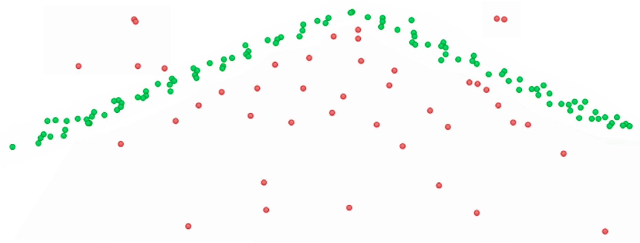
Point clouds are a simple, yet efficient, way of representing spatial data. However, despite the ease of capturing point clouds, processing them is a challenging task. Problems such as incorrectly adjusted density, clutter, occlusion, random and systematic errors, surface properties, or incorrect alignment are the main data-driven obstacles to wider dissemination, and are often related to their data structure or capture-related environmental specificities, as highlighted by F. Poux [32]. Secondly, structure-related problems usually emerge due to a lack of connectivity within point ensembles, which can render the surface information ambiguous [33]. To cope with the aforementioned problems, and obtain reliable plane estimates, the plane-extraction method should prioritize noise robustness. Indeed, ALS data sets often present high noise levels, which can become problematic for data-driven approaches (see Figure 2). In this example of a projected point cloud on a vertical plane, two kinds of noise are represented: while the red points over the roof can be explained by occluded elements (chimneys, vegetation, cables, etc.), the red points above the roof are the result of walls taken with a low-angle shot. The valid/invalid classification represents the goal of the clustering. To avoid serialization and add fragility to the proposed approach, we favor robustness over adding a pre-processing step, such as using SOR filters to filter noise beforehand.
We aim to provide an unsupervised procedure without injecting prior knowledge (whether it is from trained data or tweaking parameters). Thus, it initially focuses on extracting strict planes. To assess the impact of the shape-detection approach on our results, we implemented another unsupervised approach from [34], which was applied in an archaeological context in [35] and for indoor buildings in [36]. Its most recent overhaul (Poux et al. in press) allows for the fully unsupervised segmentation of point clouds on low-end devices.
The method scales up to billions of 3D points and targets a low-level grouping, to be independent from any application. It uses a hierarchical, multi-level segment definition to cope with potential variations in high-level object definitions. The fully unsupervised segmentation leverages planar predominance in scenes through a normal-based aggregation. For usability and simplicity, the authors designed an automatic heuristic definition for the determination of three RANSAC-inspired parameters, namely the distance threshold for the region-growing, the threshold for the minimum number of points needed to form a valid planar region, and the decisive criterion for adding points to a region. The robustness of the “one-button” method in various scenarios was tested for complex indoor buildings with different ground-sensor platforms (depth sensors, terrestrial laser scanners, hand-held laser scanners, mobile mapping systems), but not on ALS data sets. It is very robust to noise, incorrectly adjusted density, and provides a clear hierarchical point grouping, in which fully unsupervised parameter estimations give better results than “user-defined” parameters.
This process is carried out to obtain the nth point clusters, which will become the nth support for plane estimates (see Figure 3).
In this context, it is worth remembering that besides the use of an innovative method for point clouds segmentation, the improvement of each reconstruction step makes it possible to obtain a geometrically and topologically consistent model. Every step in the method is governed by normalized values and thresholds [4,5]. All these improvements make it a convincing automatic generator.
3.3. Step-By-Step Geometric Modeling
CityJSON makes it possible to structure a building geometry as a Solid, a CompositeSolid, or a MultiSurface (compliance with ISO19107 standard). Since a building delimits a volume, the solid primitive is entirely intended to fulfill this role in this method: a structured set of polygons that contain the closed volume of a rigid body. Please note that a CompositeSolid might be an improvement for buildings annexes. On the other hand, MultiSurface represent non-volumetric parts (e.g., the overhang of a roof). The goal of the building-reconstruction process is to determine the bounding polygons and the relationship between them, to produce a coherent model. The reconstruction method starts from the points, which is the information directly provided by the LiDAR point cloud. Based on the detected roof planes (in red), the footprint (in blue) is computed as the projection of roof planes. Finally, the walls (in yellow) are determined by linking every edge of the roof shape to its corresponding edge from the footprint. The Figure 4 breaks down the successive steps illustrated, by paralleling the sections and their input data.
In comparison with other hybrid approaches [29], the planes are formed via a data-driven method, but the buildings are constructed based on a connectivity graph. However, some differences should be noted: (a) the buildings are generated following the CityGML format, but the refined CityGML LoD were not taken into account in the reconstruction process [4]; (b) reconstruction steps do not follow the same phases: the primitive components (small volumes) are generated based on the Roof Topology Graph, then connected in order to generate the building model. In terms of the modeling of primitives, model-driven methods fit models to point clouds, in order to reduce metrics such as Root Mean Square Error (RMSE), Hausdorff distance (deformed shapes), tuning function distance (entire shape similarity), angle-based index, or a composition [37,38,39,40]. A particular method implements the automatic production of the CityGML model [41]. All the surfaces are semantically consistent and independent from the process (see Figure 5).
Please note that in CityJSON (because it is semi-structured), users are free to add to and modify the model, to increase its usability in dedicated applications. Further developments may pertain to the generation of other elements of the urban built environment (roads, bridges, tunnels, etc.) and the addition of specialized metadata.
3.3.1. Topology Generation
From the formed sub-sets of points, and this, the topology of the roof shape is constructed for each building. The roof shape is translated based on connections between the combinations of sub-sets. Some generalization—and therefore a loss of accuracy to the real world—must be accepted. Again, the focus is on compliance with CityGML specifications [5]. Therefore, some thresholds need to be established, as they are provided in the standard (e.g., minimum slope of 5°, in order to differentiate planes, and a minimum area of six square meters for Buildings).
The different sub-sets of points are projected onto a virtual XY horizontal plane. The minimum oriented bounding box is computed based on the coordinates of the points that comprise the sub-set. This polygon gives us the oriented sub-footprint determined by the plane (i.e., the oriented envelope that forms the minimum extent of a two-dimensional set of points). The connections between the different sub-footprints are considered between pairs: if the intersection line occurs within the footprint polygon, and if the intersection is consistent with the connectivity graph, the new connection is added to the topology graph.
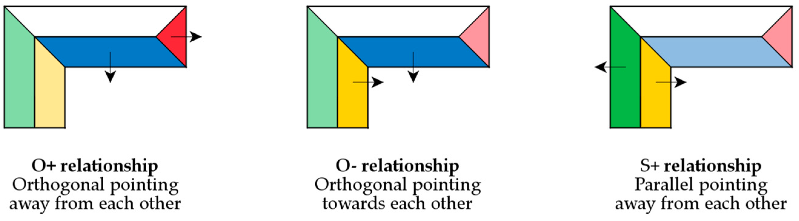
The nature of the relationship will influence the connectivity and its physical representation (valleys, hips, and ridges). The plane relationship can be classified into three constrained families and one default one [42]:
- O+ planes have normal vectors that when projected, are orthogonal and point away from each other.
- O- planes have normal vectors that when projected, are orthogonal and point towards each other.
- S+ planes have normal vectors that when projected, are parallel and point away from each other.
- N = no constraint.
Please note that the notion of the connectivity graph is part of hybrid-driven modeling [3]: the Roof Attribute Graph (RAG) [43], the Region Adjacency Graph [44], or the Roof Topology Graph [45]. The main difference with these graphs lies in the handling of parallelism: The S+ class, which is not present in other methods, provides additional information. To determine orthogonality and parallelism, the normal vectors are projected onto the XY plane. Based on a threshold of 5°, the angle between them determines the relationships [5]. We assume that the method provides a good balance between the flexibility of the reconstruction methods and the quality of the reconstructed-building models. The different families are illustrated in Figure 6:
Since the N family does not provide any information, it is not stored. The assumption is made based on the absence of information. From here, the relationship can be used to determine what this relationship consists of, materially speaking. For instance, from a S+ relationship, one can state that the roof skeleton comprises at least one line segment and two points. Conversely, O relationships provide a point for the roof skeleton. This information will be further used in the roof-reconstruction process. Please note that an empty graph will lead to a composition of flat or lean-to roofs. Breaking down the graph can also be easily used to simplify shapes or extract a subpart of a building. The connectivity information is computed on a couple of planes. As a result, this information can easily be stored in two matrices:
- An adjacency matrix (i, j), which contains the ID of j planes connected to the i plane.
- A relationship matrix, which contains the nature of the connectivity between the i and j planes.
From the connectivity graph, if two planes are connected, the footprint is, at least, the union of both. The process loops iteratively above the upper diagonal of the adjacency matrix and constructs the footprint as it goes. Once the graph has been traveled, the polygon is generalized, by computing the concave hull of the various elements to get a coherent polygon. The concave hull is significant, given that L, U, etc. shaped buildings should not be closed. Thresholds that comply with CityGML specifications are applied, in order to ensure the consistency of the footprint and clean potential errors [30].
The result provides a flying footprint (i.e., the projected envelope of the building, without elevation). This envelope is part of the 3D bounding box of the building. The lowest Z limit can be determined, thanks to the digital elevation model (DEM) generated from the airborne point cloud. It is provided with the point cloud and the results of the triangulation of the “ground” points from the LASer format classification (LAS). This elevation model has an altimeter accuracy of 0.12 m and a spatial resolution of 1 m. The last coordinate of the box, i.e., its elevation, is calculated as part of the roof generation.
3.3.2. Roof Generation
Unless planes are perfectly parallel, two planes always intersect somewhere. This connection needs to be within the footprint, to be part of the skeleton. Otherwise, it could cause inconsistencies: irrelevant rupture lines will degrade the representation of the roof shape. Afterwards, all combinations of lines are computed traveling along the topology graph. For S+ relationships (and only S+ relationships), the intersection points for these lines with the footprint are also determined. For instance, this is the case for the ridge of gable roofs, as shown by the yellow plane in Figure 7. According to the CityGML specifications [5], a threshold of two meters snaps the rupture points to those that have previously extruded from the footprint. This perfect snapping tolerance increases confidence in the model topology. Hence, it prevents holes (see the introduction for an explanation). The rupture points form the outline of the roof. The lines and rupture points are stored in a rupture matrix, similar to the adjacency and relationship matrices.
Finally, the points of intersection between the rupture lines are determined and added to the rupture points. Their heights are interpolated afterwards. Please note that in cases where there is no intersection between roof planes in the footprint polygon, this means that the roof is flat or lean-to shaped. In this case, the building model cannot be refined further. Only the LoD 1.x will be generated for these buildings. Even if this kind of shape has already been detected, a second filter is applied to ensure they are detected.
Roof planes are built while traveling segment-by-segment through the footprint. For each point, the orthogonal distances to the roof planes are computed through the normal vectors. Since a point from the outline of a roof is part of two roof planes, the two lesser distances determine the plane to which they belong. After this, the non-intersecting polygon is computed for each roof plane, by considering these points and the results stored in the rupture matrix. This polygon results from sorting two sub-sets of points and drawing the line that links the left-most and right-most point. The non-intersecting polygon is the concatenation of the points that are higher than the line and those that are lower, sorted from left to right and vice versa (see Figure 8 for an illustration). It should be mentioned that the concave hull of a set of points tends to determine the smallest polygon that links all the points. This smallest polygon is not always the correct representation of the wall in cases with very sharp angles.
To conclude with roof planes, the height of the points is calculated according to the plane equations. Since each vertex belongs to several planes, an arithmetic mean gives its height. Please note that this operation corrupts the planarity of the different plans. An issue with non-planarity could lead to problems when calculating surface areas, for instance. However, this operation distributes the errors evenly. The denser and less noisy the point cloud, the more accurate the reconstruction. Finally, the highest point of the LoD 2.x building model gives the height of its 3D bounding box.
3.3.3. Wall Generation
This module is simpler than the two previous modules, as it only binds results to results. As well as roof planes, walls are generated while traveling segment-by-segment through the footprint. The intersections of segments with projected roof planes are computed. The vertices of the intersection, and those that are extracted from the footprint segment, give the points that delimit the wall. Once more, the non-intersecting polygon is determined and provides the sorted vertices that draw the wall parts.
A general remark concerns all three modules. When rendering the rigid body via back-face culling, a unique rule is applied: the normal vector should point towards the outside of the volume. This translates into the order of vertices for each surface. This needs to be counterclockwise and ordered from an exterior viewpoint. All faces are controlled under these conditions. Otherwise, the volumes are closed, but their display, among other things, may appear problematic. This depends on the viewer and the application (see Figure 9 for an illustration).
3.3.4. Building Assembly
A building comprises a Solid bounding a closed volume. Again, the nature of the surfaces is not inferred from their slope, orientation, or position, but by the process: the footprint is always the first element generated, then roof planes, and walls close the 3D geometry (Refer to Figure 10 for the construction order: red, then blue, then yellow). The three possibilities (GroundSurface, WallSurface, or RoofSurface) are listed and mapped into an array, which corresponds to the order of the different planes. This information is stored within the JSON objects as the semantics JSON key within each building object. The polygons that define the different planes are stored as sorted arrays of the vertices’ identifiers. They constitute the boundaries of the JSON object.
CityJSON allows objects to be represented in concurrent LoD. Since not all applications need a detailed level of design, the three LoD are produced. They represent stages from the footprint to the roof-shaped geometries (see Figure 10 for an illustration). The sub-levels (LoD 0.x and LoD 1.x) do not require additional processing: the footprint and the bounding box are already determined beforehand. Those are stored as the 0.1 and 1.1 level of the building [46], respectively. Please note that there are multiple ways to determine the elevation of the extruded solid: minimum, maximum, mean, and median. In this case, however, using the maximum elevation seems to be the most conservative approach for defining a volume.
3.4. CityJSON Model Building
The CityJSON model is created on an iterative basis through this process. The specifications require some JSON keys to be present in every file: type, version, CityObjects, and vertices. Although type and version are easily created, CityObjects and vertices require an explanation. CityObjects represents the concatenation of all Building objects created in the previous section, with their own boundaries, semantics, etc. Next to this, the coordinates for the vertices are stored in bulk at the end of the city-model file. They are stored in the order of their identifiers (i.e., their successive creation). This method makes it possible to reduce the size of the model and avoid redundant information, even if this redundancy is still allowed in the CityJSON specifications. Nonetheless, it is an additional, necessary condition for building a compact city model. Moreover, the optional transform JSON key allows the coordinates of the vertices to be decompressed, to improve the compactness of the model, as is already done in TopoJSON.
Another important element pertains to metadata. Due to their importance and the impact of their support, this element will be extensively discussed in the next section.
An example of a CityJSON-generated model is shown in Figure 11. The point cloud and the reconstruction are displayed one after another in the CloudCompare viewer, in the open-source viewer developed at the 3D GeoInformation group from TUDelft (https://github.com/tudelft3d/CityJSON-viewer/) and an open-source extension of Cesium (https://github.com/limyyj/cesium-cityjson). A quick glance shows that pyramidal and more complex shapes are represented within the data, even if gable roof shapes represent the majority.
4. Discussion
This section discusses the advantages of directly generating CityJSON models and assesses the quality of the results using several normalized and formal tools. The first part of this section develops the research contribution of this paper, then the second section makes it possible to rule on the validity of the geometrical reconstruction in comparison with the state-of-the-art approach. First, compliance with CityGML/CityJSON specifications is evaluated; the geometric validity of every building is also studied.
4.1. CityJSON Improvements
From a conceptual perspective, CityGML and CityJSON are not different. On a global level, the construction of a model could be done in parallel for both formats. A geometry comprising edges and vertices can be formatted in either CityGML or CityJSON without any loss or inaccuracy. Consequently, the translation between them both is not a problem, but it is not direct one-to-one mapping. Even if they share the same conceptual schema, several notable differences exist in their descriptive components. For instance, CityJSON makes it possible to manage two additional elements in particular: (a) the ability to handle metadata natively [6] and (b) the refined LoD [4]. By providing a method that breaks down geometric reconstruction, and working on improvements to every constituent part, we manage both (a) and (b) points during the process.
CityJSON offers the ability to handle metadata natively. Conversely, CityGML requires the use of an extension for managing metadata [6]. For that reason, translation from CityGML to CityJSON, and vice versa, cannot occur without a loss of information. Taking the example of the command-line translator from CityGML to CityJSON, the information is simply neglected if it is not part of the destination format. The proposal of a generation method that directly offers a CityJSON model responds to this problem. It makes it possible to avoid such a loss.
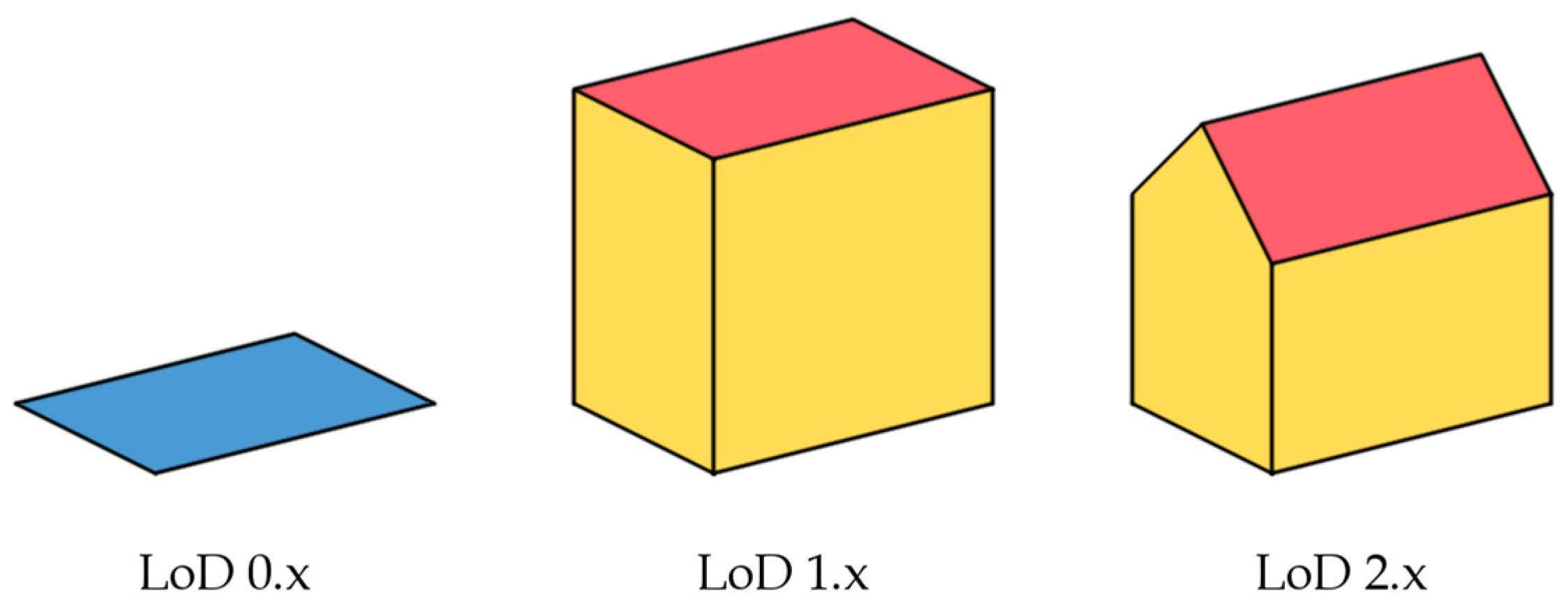
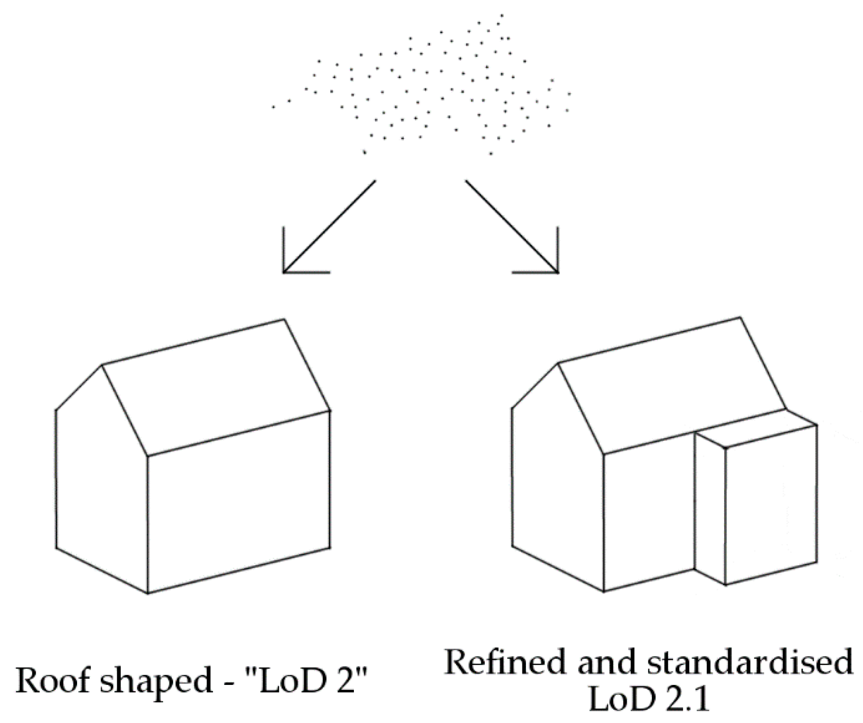
On one hand, the refined level-of-detail definitions, and their related metrics, are managed. Throughout the generation process, thresholds are provided, and we guarantee compliance with specifications. In this case, we managed to create 0.1, 1.1, and 2.1 LoD concurrently [4]. A related benefit is that we can store all the levels at the same time. Moreover, these levels are interdependent, since the footprint—the actual 0.1 LoD—is the basement of the 1.1 and 2.1 LoDs. These improved definitions provide important information about the form factor of the building, which is not allowed in common LoDs. The refined LoDs do not only show individual and large building parts, but also small building parts, recesses, and extensions. Figure 12 depicts a comparison between common LoDs, which provide minimal specs, and refined LoDs, which provide improved conception of details. Therefore, it allows applications to make the choice of the more relevant level for their scope of interest. From a user perspective, i.e., fluid-flow simulations, this level of detail in building has an important impact [24].
In terms of contextual information, it is possible to compute and handle metadata during the process. Among other things, CityJSON makes it possible to manage the geographical extent of the city. In addition to the geometry of a building, its geographical extent is computed simultaneously (i.e., the minimum oriented and bounding cuboid). The choice has been made to consider the maximum height of the building, to be on the safe side and not underestimate the influence of elements on their built environment. Finally, the extent of buildings can be aggregated to determine the geographic extent of the whole city model. This extent is then stored in the model metadata, which is not available in a built-in manner in CityGML (see Figure 13). Moreover, the lack of CityGML ISO19115 support is detrimental when it comes to exchanging information, comparing concurrent models for the same element, or keeping a record of the model versioning. As a reminder, the starting hypothesis is to provide a compact model that allows easy online exchanges. Thanks to CityJSON and this method, ambiguity is no longer possible.
4.2. Format Compliance
CityJSON specifications provide a sub-set of the CityGML data model [7]. JSON, as opposed to XML, has the advantage of not using end tags, which reduce format redundancies; it does not require the repetition of information for each element when handling arrays; etc. However, both share many similarities, which make them primary formats for exchanging data online: (i) they are both self-describing, (ii) hierarchical, and (iii) fetched within HTTP requests. The JSON hierarchy is structured as nested key-value pairs (i.e., a map), while XML is structured as a tree. This is the main reason trees can be tedious and time-consuming to parse. In short, XML is better for storing information—thanks to namespaces—and JSON is better for delivering data, thanks to its compactness.
From a format point of view, it is, therefore, important for the generated model to be compliant with the official CityJSON schemas. To ensure this compliance, a Command-Line Interface (CLI) provided by TUDelft makes it possible to validate and transform CityJSON files (https://github.com/cityjson/cjio). No error has been detected through our various tests with the CLI (vertex indices coherent, specifics for CityGroups, semantic arrays coherent with geometry, root properties, empty geometries, duplicate vertices, orphan vertices, CityGML attributes). This is easily explained as follows: every individual inconsistency is handled upstream within our software.
4.3. Quality Control
Every individual vertex could lead to local singularities in the topological consistency during the reconstruction process. Two sub-processes prevent this from happening and ensure that buildings are closed: vertices generalization and perfect snapping tolerance [5]. Both methods are informed by the geometric specifications of the refined LoDs in CityGML [4], which state that building parts that are smaller than two square meters wide should be generalized and that two vertices that are less than two meters apart are considered to be the same vertex on the XY plane. Please note that the generalization happens during the footprint establishment, when vertices do not yet exist, but the snapping happens later, during the creation of the wall, roof, and footprint, when vertices do exist.
4.3.1. Spatio-Semantic Evaluation
Semantic validity is crucial: little room is left for semantic uncertainty. Again, the nature of the surfaces is not inferred from the normal orientation or relative positions, but during the process: the footprint is always the first element generated; roof planes are generated from their connectivity graph and, finally, wall planes are created. Spatio-semantic validity is therefore easy to obtain.
Given that CityGML has become the de facto standard for spatio-semantic city modeling, the Interoperability Experiments Joint Activity between OGC, SIG3D, and EuroSDR defined some requirements in order to normalize its use. The OGC IEJA group conducts research and provides tools to carry out quality assurance on the data, including data used in this research. Their discussions about issues relating to CityGML data quality has led to usage guidelines [28]: (i) a definition of data quality, (ii) data-quality requirements and their specification, (iii) a quality-checking process for CityGML data, and (iv) a description of validation results.
4.3.2. Geometric Evaluation
The main idea is to simplify validation by cascading it: we must validate the previous steps before proceeding to the next step. Therefore, if a critical geometric inconsistency has been detected, no semantic validation should be carried out [47]. Recently, new tools are proposing the management of more discrete LoD: previous tools were limited at levels close to LoD1.x (flat roofs and vertical walls). A standard-error taxonomy is necessary to help structure the evaluation. From the intrinsic features of the models, errors can be detected using a supervised classifier (e.g., random forest) [48,49]. However, this does not support CityJSON. Our methodology was validated with the versatile val3dity tool [50]. Complex geometries are systematically broken down into their constituent parts: the integrity of buildings is processed, then every 3D primitive is validated. Here, it is worth mentioning that overlapping—as it is implemented in val3dity—considers relations between BuildingParts and not between Buildings and each other. This is an important point regarding computation time, as overlapping greatly slows down the process: the Minkowski sum is used to assess overlaps. It has O(n3m3) run-time complexity, where n is the number of objects and m the number of constituent parts therein [51]. As is the case for CityGML, only planar and linear primitives are allowed: cylinders, spheres, or other curved, parametrically modeled primitives are not supported. The validation parameters in the val3dity tool are as follows [50]:
- Snap tolerance: 0.001 m—if two points are closer than this value, then they are assumed to be the same.
- Planarity tolerance: 0.05 m—the maximum distance between a point and a fitted plane.
- Overlap tolerance: 0.01 m—the tolerance used to validate adjacency between different solids.
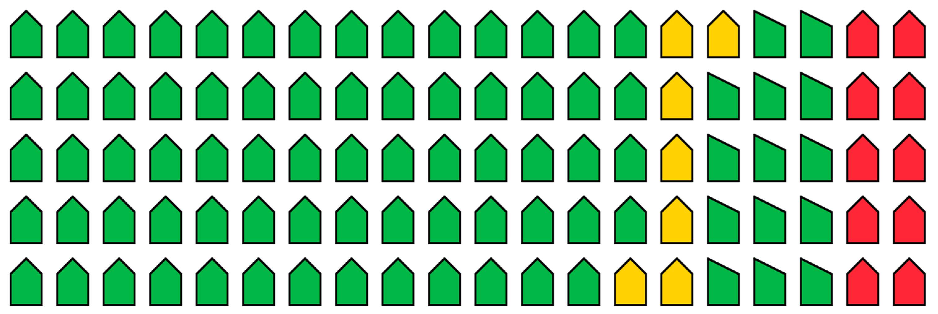
Figure 14 provides a graphical overview of the results for the city of Theux in Belgium. Please note that the definition of “Building” itself might differ between standards and applications, especially for LiDAR point clouds, since they are not initially intended to suit CityGML definitions. Hence, some elements do not belong to the CityGML definition. For the remainder, the footprint of a Building element needs to be greater than six square meters. The red buildings in Figure 14 represents these elements scaled onto 100 buildings. This proportion represents 44 buildings from the complete set (464 elements). On the other hand, 65 buildings are classified as flat or lean-to roofs (green buildings on the right of Figure 14). They are thus not included in the LoD2.x reconstruction benchmark. Finally, the buildings that correspond to complex roof shapes are validated. In the end, 31 buildings are not validated from the 355 remaining buildings (yellow buildings in Figure 14). This corresponds to 91.26% validity for the LoD2.x objects, i.e., most of the data set is valid. The Buildings that could not be reconstructed in LoD2.x are instead generated as LoD0.x and LoD1.x (footprint and extruded volumes).
The results provided by our methodology have been compared to open data sets (see Table 1) [50]. Overall, the proposed methodology provides a ratio of valid/invalid geometries of over 90%. Please note that the other benchmarked data concern CityGML files. No other information about the source and/or creation of the data was given. The increasing validity from Buildings to Primitives is explained by the fact that lower LoDs are easier to generate.
The difference in building numbers between the unsupervised RANSAC (UR) and the region-growing (RG) stems from pre-processing (removal of statistical outliers, clustering, etc.). Indeed, the point cluster does not always satisfy the requirements to be considered to be Buildings, as per CityGML specifications. Here, the assumption that segmentation is effective shows its limitations: if planes are not detected, or they overlap too much, the connectivity graph will not be correct. The proposed methodology partially relies on the restrictive hypothesis that the segmentation properly detects the planes. When analyzing the results, the main source of errors currently stems from the segmentation methods and the low point density. The val3dity tool provides a taxonomy of errors that could be encountered during a geometric evaluation [50]. In the successive development phases, only one recurrent sub-set of these errors was detected—non-planar polygon distance—since the algorithm already prevents many of them.
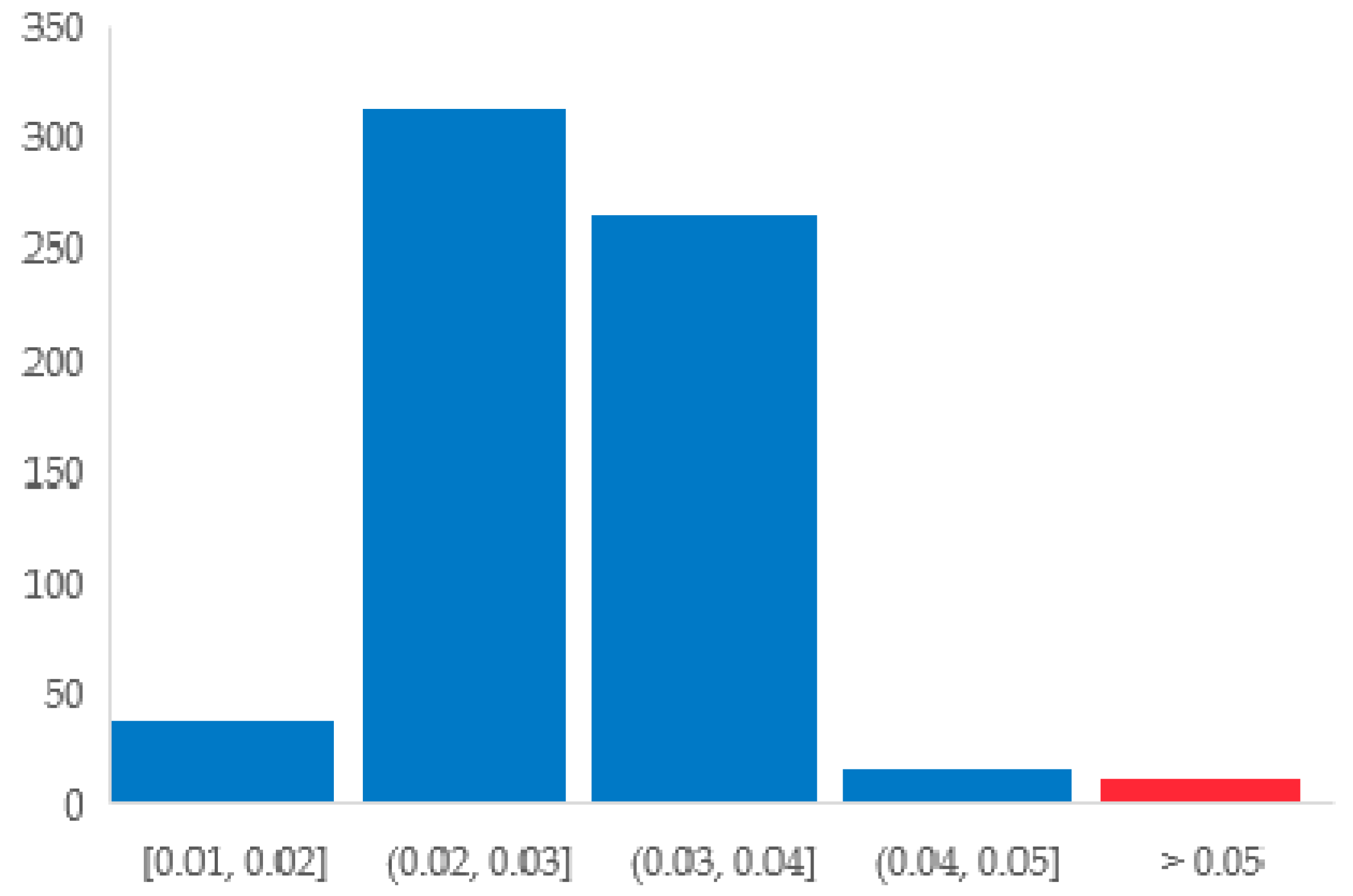
Nevertheless, the distribution of these errors only deviates slightly from the theoretical threshold of 5 cm. Only a few of them stand out. It is also essential to mention that the plane-interpolation algorithms are different between val3dity (least mean squares) and the methodology (RANSAC) [19]. To assess the quality of the plane interpolation, the RMSE of each roof plane for the Z-axis is computed (see Figure 15 for error classes). As can be seen, the distribution of errors tends to be close to 3 cm (median: 0.028 m, 95th percentile: 0.039 m). Only 8 of the 644 planes have an RMSE greater than 5 cm (these are actually outliers greater than 2 m).
However, one negative point should be noted: even if the number of buildings affects the processing time on a linear basis, RANSAC is still the primary source of time complexity. Taking this consideration into account, two features influence the processing time: the ratio of points within the sub-set and the total number of points [52]. Therefore, filtering the point cloud is mandatory. We tested filtering versus not filtering the data provided. The use of the SOR filter corresponds to an improvement of 30% to the computation time. Another improvement of our method is the use of a k-d tree index, rather than an octree, for identifying point neighbors. This was done in order to reduce the number of spurious planes during segmentation [19].
Buildings are not always made up of a single volume: some have annexes and outbuildings. Considering these additional parts in the reconstruction could greatly enhance the applicability of the models. In particular, this could improve land administration and cadaster applications. Considering this, a further interesting development could use a CompositeSolid construction (i.e., the aggregation of one or more Solids—a non-empty set of Solids). Special attention will need to be paid to the topology of Solids. Independent management of floors could also be considered in line with this new management of parts.
Currently, if an LoD2.x geometry is deemed inconsistent, the generation is limited to lower levels. It could be interesting to fill the potentially detected holes, rather than treating the geometry as corrupted. For example, one can use a top-down, shrink-wrapping process to re-mesh the polygonal surfaces [53], or reconstruct these missing planes directly within the connectivity graph [43]. As this makes it possible to repair common errors and fill holes (windows and doors), the integrity of LoD 2.x objects would be respected, although this envelope might smooth geometric details.
5. Conclusions
This paper aims to respond to the lack of availability and versatility of 3D City models, by providing a simplistic method for generating city buildings. Besides this, thanks to the use of CityJSON and the break-down of reconstruction methods, the integration of metadata and refined LoD are now supported within the generation process. The presented methodology does not rely on commercial or proprietary solutions. We believe that the opening up of our straight-generation method will help to disseminate the use of CityJSON. It will also facilitate further related works in the context of the urban built environment. The evaluation and comparison, which is based on the validity rate of the geometries generated (format, semantic, and topologic validity), showed that it is possible to automatically reconstruct LoD2.x buildings based on LiDAR data and CityGML/CityJSON specifications.
In terms of format and semantic validity, no error has been encountered. The provided city models are consistent, in every respect, with the standard specifications. Two methods were tested for plane detection: an unsupervised RANSAC and a fully unsupervised, normal-vector-based RG algorithm. Although the RANSAC method needed minimal tuning for its hyper-parameters, the second method determined ideal clusters without input parameters. A significant ancillary result of this work is the use of indoor point-cloud segmentation in an outdoor context. As it pertains to geometries, the quality is assessed on a normalized basis, thanks to formal tools such as CJIO and val3dity. The ratio of valid/invalid buildings varies between 92% and 97%, depending on the segmentation method. Several improvements are considered, including the addition of elements of urban landscapes (roads, etc.).
Author Contributions
Conceptualization, Gilles-Antoine Nys; methodology, Gilles-Antoine Nys and Florent Poux; software, Gilles-Antoine Nys; validation, Gilles-Antoine Nys; formal analysis, Gilles-Antoine Nys; investigation, Gilles-Antoine Nys; resources, Gilles-Antoine Nys and Florent Poux; data curation, Gilles-Antoine Nys; writing—original draft preparation, Gilles-Antoine Nys; writing—review and editing, Gilles-Antoine Nys, Florent Poux and Roland Billen; visualization, Gilles-Antoine Nys; supervision, Roland Billen. All authors have read and agreed to the published version of the manuscript.
Funding
This research received no external funding.
Acknowledgments
We acknowledge the availability of the data sets from the following sources: Service Public de Wallonie (Walloon Public Services).
Conflicts of Interest
The authors declare no conflict of interest.
References
- Billen, R.; Cutting-Decelle, A.-F.; Marina, O.; de Almeida, J.-P.; Caglioni, M.; Falquet, G.; Leduc, T.; Métral, C.; Moreau, G.; Perret, J.; et al. (Eds.) 3D City Models and Urban Information: Current Issues and Perspectives: European COST Action TU0801; EDP Sciences: Liège, Belgium, 2014; pp. 1–118. [Google Scholar]
- Gröger, G.; Plümer, L. CityGML—Interoperable semantic 3D city models. ISPRS J. Photogramm. Remote Sens. 2012, 71, 12–33. [Google Scholar] [CrossRef]
- Wang, R.; Peethambaran, J.; Chen, D. LiDAR Point Clouds to 3D Urban Models: A Review. IEEE J. Sel. Top. Appl. Earth Obs. Remote Sens. 2018, 11, 606–627. [Google Scholar] [CrossRef]
- Biljecki, F.; Ledoux, H.; Stoter, J. An improved LOD specification for 3D building models. Comput. Environ. Urban Syst. 2016, 59, 25–37. [Google Scholar] [CrossRef] [Green Version]
- Biljecki, F.; Ledoux, H.; Du, X.; Stoter, J.; Soon, K.H.; Khoo, V.H.S. The most common geometric and semantic errors in CityGML datasets. ISPRS Ann. Photogramm. Remote Sens. Spat. Inf. Sci. 2016, 4, 13–22. [Google Scholar] [CrossRef] [Green Version]
- Labetski, A.; Kumar, K.; Ledoux, H.; Stoter, J. A metadata ADE for CityGML. Open Geospat. Data Softw. Stand. 2018, 3, 16. [Google Scholar] [CrossRef] [Green Version]
- Ledoux, H.; Ohori, K.A.; Kumar, K.; Dukai, B.; Labetski, A.; Vitalis, S. CityJSON: A compact and easy-to-use encoding of the CityGML data model. Open Geospat. Data Softw. Stand. 2019, 4, 4. [Google Scholar] [CrossRef]
- Tarsha Kurdi, F.; Awrangjeb, M. Automatic evaluation and improvement of roof segments for modelling missing details using Lidar data. Int. J. Remote Sens. 2020, 41, 4702–4725. [Google Scholar] [CrossRef]
- Poux, F.; Hallot, P.; Neuville, R.; Billen, R. Smart Point Cloud: Definition and Remaining Challenges. ISPRS Ann. Photogramm. Remote Sens. Spat. Inf. Sci. 2016, 4, 119–127. [Google Scholar] [CrossRef] [Green Version]
- Lafarge, F.; Mallet, C. Creating Large-Scale City Models from 3D-Point Clouds: A Robust Approach with Hybrid Representation. Int. J. Comput. Vis. 2012, 99, 69–85. [Google Scholar] [CrossRef]
- Jung, J.; Sohn, G. A line-based progressive refinement of 3D rooftop models using airborne LiDAR data with single view imagery. ISPRS J. Photogramm. Remote Sens. 2019, 149, 157–175. [Google Scholar] [CrossRef]
- Zhou, K.; Lindenbergh, R.; Gorte, B.; Zlatanova, S. LiDAR-guided dense matching for detecting changes and updating of buildings in Airborne LiDAR data. ISPRS J. Photogramm. Remote Sens. 2020, 162, 200–213. [Google Scholar] [CrossRef]
- Cao, R.; Zhang, Y.; Liu, X.; Zhao, Z. 3D building roof reconstruction from airborne LiDAR point clouds: A framework based on a spatial database. Int. J. Geogr. Inf. Sci. 2017, 31, 1359–1380. [Google Scholar] [CrossRef]
- Schnabel, R.; Wahl, R.; Klein, R. Efficient RANSAC for Point-Cloud Shape Detection. Comput. Graph. Forum 2007, 26, 214–226. [Google Scholar] [CrossRef]
- Ballard, D.H. Generalizing the Hough Transform to Detect Arbitrary Shapes. In Readings in Computer Vision; Elsevier: Oxford, UK, 1987; pp. 714–725. ISBN 978-0-08-051581-6. [Google Scholar]
- Borrmann, D.; Elseberg, J.; Lingemann, K.; Nüchter, A. A Data Structure for the 3D Hough Transform for Plane Detection. IFAC Proc. Vol. 2010, 43, 49–54. [Google Scholar] [CrossRef]
- Liu, X.; Zhang, Y.; Ling, X.; Wan, Y.; Liu, L.; Li, Q. TopoLAP: Topology Recovery for Building Reconstruction by Deducing the Relationships between Linear and Planar Primitives. Remote Sens. 2019, 11, 1372. [Google Scholar] [CrossRef] [Green Version]
- Tarsha-Kurdi, F.; Landes, T.; Grussenmeyer, P. Hough-Transform and Extended RANSAC Algorithms for Automatic Detection of 3D Building Roof Planes from Lidar Data. In Proceedings of the ISPRS Workshop on Laser Scanning 2007 and SilviLaser 2007, Espoo, Finland, 12–14 September 2007; pp. 407–412. [Google Scholar]
- Li, L.; Yang, F.; Zhu, H.; Li, D.; Li, Y.; Tang, L. An Improved RANSAC for 3D Point Cloud Plane Segmentation Based on Normal Distribution Transformation Cells. Remote Sens. 2017, 9, 433. [Google Scholar] [CrossRef] [Green Version]
- Xu, B.; Jiang, W.; Shan, J.; Zhang, J.; Li, L. Investigation on the Weighted RANSAC Approaches for Building Roof Plane Segmentation from LiDAR Point Clouds. Remote Sens. 2015, 8, 5. [Google Scholar] [CrossRef] [Green Version]
- Pârvu, I.M.; Remondino, F.; Ozdemir, E. LoD2 Building Generation Experiences and Comparisons. J. Appl. Eng. Sci. 2018, 8, 59–64. [Google Scholar] [CrossRef] [Green Version]
- Rottensteiner, F.; Sohn, G.; Gerke, M.; Wegner, J.D.; Breitkopf, U.; Jung, J. Results of the ISPRS benchmark on urban object detection and 3D building reconstruction. ISPRS J. Photogramm. Remote Sens. 2014, 93, 256–271. [Google Scholar] [CrossRef]
- Awrangjeb, M.; Gilani, S.; Siddiqui, F. An Effective Data-Driven Method for 3-D Building Roof Reconstruction and Robust Change Detection. Remote Sens. 2018, 10, 1512. [Google Scholar] [CrossRef] [Green Version]
- Kumar, K.; Ledoux, H.; Stoter, J. Dynamic 3D Visualization of Floods: Case of the Netherlands. ISPRS Int. Arch. Photogramm. Remote Sens. Spat. Inf. Sci. 2018, 42, 83–87. [Google Scholar] [CrossRef] [Green Version]
- Kumar, K.; Labetski, A.; Ohori, K.A.; Ledoux, H.; Stoter, J. The LandInfra standard and its role in solving the BIM-GIS quagmire. Open Geospat. Data Softw. Stand. 2019, 4, 5. [Google Scholar] [CrossRef] [Green Version]
- Vitalis, S.; Ohori, K.; Stoter, J. Incorporating Topological Representation in 3D City Models. ISPRS Int. J. Geo-Inf. 2019, 8, 347. [Google Scholar] [CrossRef] [Green Version]
- Huang, H.; Brenner, C.; Sester, M. A generative statistical approach to automatic 3D building roof reconstruction from laser scanning data. ISPRS J. Photogramm. Remote Sens. 2013, 79, 29–43. [Google Scholar] [CrossRef]
- Wagner, D.; Ledoux, H. CityGML Quality Interoperability Experiment; OGC: Wayland, MA, USA, 2016. [Google Scholar]
- Wichmann, A. Grammar-guided reconstruction of semantic 3D building models from airborne LiDAR data using half-space modeling. Comput. Sci. 2018. [Google Scholar] [CrossRef]
- Fan, H.; Meng, L. A three-step approach of simplifying 3D buildings modeled by CityGML. Int. J. Geogr. Inf. Sci. 2012, 26, 1091–1107. [Google Scholar] [CrossRef]
- Balta, H.; Velagic, J.; Bosschaerts, W.; De Cubber, G.; Siciliano, B. Fast Statistical Outlier Removal Based Method for Large 3D Point Clouds of Outdoor Environments. IFAC-PapersOnLine 2018, 51, 348–353. [Google Scholar] [CrossRef]
- Poux, F. The Smart Point Cloud: Structuring 3D Intelligent Point Data; Université de Liège: Liège, Belgique, 2019. [Google Scholar]
- Berger, M.; Tagliasacchi, A.; Seversky, L.M.; Alliez, P.; Guennebaud, G.; Levine, J.A.; Sharf, A.; Silva, C.T. A Survey of Surface Reconstruction from Point Clouds. Comput. Graph. Forum 2017, 36, 301–329. [Google Scholar] [CrossRef] [Green Version]
- Poux, F.; Billen, R. Voxel-Based 3D Point Cloud Semantic Segmentation: Unsupervised Geometric and Relationship Featuring vs. Deep Learning Methods. ISPRS Int. J. Geo-Inf. 2019, 8, 213. [Google Scholar] [CrossRef] [Green Version]
- Poux, F.; Neuville, R.; Van Wersch, L.; Nys, G.-A.; Billen, R. 3D Point Clouds in Archaeology: Advances in Acquisition, Processing and Knowledge Integration Applied to Quasi-Planar Objects. Geosciences 2017, 7, 96. [Google Scholar] [CrossRef] [Green Version]
- Poux, F.; Billen, R. A Smart Point Cloud Infrastructure for intelligent environments. In Laser Scanning; Riveiro, B., Lindenbergh, R., Eds.; CRC Press: Boca Raton, FL, USA, 2019; pp. 127–149. ISBN 978-1-351-01886-9. [Google Scholar]
- Dorninger, P.; Pfeifer, N. A Comprehensive Automated 3D Approach for Building Extraction, Reconstruction, and Regularization from Airborne Laser Scanning Point Clouds. Sensors 2008, 8, 7323–7343. [Google Scholar] [CrossRef] [Green Version]
- Kada, M.; McKinley, L. 3D Building reconstruction from LiDAR based on a cell decomposition approach. Int. Arch. Photogramm. Remote Sens. Spat. Inf. Sci. 2009, 38, 47–52. [Google Scholar]
- Huang, H.; Mayer, H. Towards Automatic Large-Scale 3D Building Reconstruction: Primitive Decomposition and Assembly. In Societal Geo-Innovation; Bregt, A., Sarjakoski, T., Van Lammeren, R., Rip, F., Eds.; Springer International Publishing: Cham, Switzerland, 2017; pp. 205–221. ISBN 978-3-319-56758-7. [Google Scholar]
- Jung, J.; Jwa, Y.; Sohn, G. Implicit Regularization for Reconstructing 3D Building Rooftop Models Using Airborne LiDAR Data. Sensors 2017, 17, 621. [Google Scholar] [CrossRef] [PubMed]
- Henn, A.; Gröger, G.; Stroh, V.; Plümer, L. Model driven reconstruction of roofs from sparse LIDAR point clouds. ISPRS J. Photogramm. Remote Sens. 2013, 76, 17–29. [Google Scholar] [CrossRef]
- Verma, V.; Kumar, R.; Hsu, S. 3D Building Detection and Modeling from Aerial LIDAR Data. In Proceedings of the 2006 IEEE Computer Society Conference on Computer Vision and Pattern Recognition, New York, NY, USA, 17–22 June 2006; Volume 2, pp. 2213–2220. [Google Scholar]
- Hu, P.; Yang, B.; Dong, Z.; Yuan, P.; Huang, R.; Fan, H.; Sun, X. Towards Reconstructing 3D Buildings from ALS Data Based on Gestalt Laws. Remote Sens. 2018, 10, 1127. [Google Scholar] [CrossRef] [Green Version]
- Milde, J.; Zhang, Y.; Brenner, C.; Plümer, L.; Sester, M. Building reconstruction using a structural description based on a formal grammar. Int. Arch. Photogramm. Remote Sens. Spat. Inf. Sci. 2008, 37, 47. [Google Scholar]
- Xiong, B.; Jancosek, M.; Oude Elberink, S.; Vosselman, G. Flexible building primitives for 3D building modeling. ISPRS J. Photogramm. Remote Sens. 2015, 101, 275–290. [Google Scholar] [CrossRef]
- Biljecki, F.; Ledoux, H.; Stoter, J.; Zhao, J. Formalisation of the level of detail in 3D city modeling. Comput. Environ. Urban Syst. 2014, 48, 1–15. [Google Scholar] [CrossRef] [Green Version]
- Wagner, D.; Wewetzer, M.; Bogdahn, J.; Alam, N.; Pries, M.; Coors, V. Geometric-Semantical Consistency Validation of CityGML Models. In Progress and New Trends in 3D Geoinformation Sciences; Pouliot, J., Daniel, S., Hubert, F., Zamyadi, A., Eds.; Springer: Berlin/Heidelberg, Germany, 2013; pp. 171–192. ISBN 978-3-642-29792-2. [Google Scholar]
- Ennafii, O.; Bris, A.L.; Lafarge, F.; Mallet, C. Semantic Evaluation of 3D City Models. Unpublished work. 2018. [Google Scholar] [CrossRef]
- Ennafii, O.; Le Bris, A.; Lafarge, F.; Mallet, C. A Learning Approach to Evaluate the Quality of 3D City Models. Photogramm. Eng. Remote Sens. 2019, 85, 865–878. [Google Scholar] [CrossRef] [Green Version]
- Ledoux, H. Val3dity: Validation of 3D GIS primitives according to the international standards. Open Geospat. Data Softw. Stand. 2018, 3, 1. [Google Scholar] [CrossRef]
- Hachenberger, P.; Kettner, L.; Mehlhorn, K. Boolean operations on 3D selective Nef complexes: Data structure, algorithms, optimized implementation and experiments. Comput. Geom. 2007, 38, 64–99. [Google Scholar] [CrossRef] [Green Version]
- Raguram, R.; Chum, O.; Pollefeys, M.; Matas, J.; Frahm, J.-M. USAC: A Universal Framework for Random Sample Consensus. IEEE Trans. Pattern Anal. Mach. Intell. 2013, 35, 2022–2038. [Google Scholar] [CrossRef] [PubMed]
- Zhao, Z.; Ledoux, H.; Stoter, J. Automatic Repair of Citygml Lod2 Buildings Using Shrink-Wrapping. ISPRS Ann. Photogramm. Remote Sens. Spat. Inf. Sci. 2013, 309–317. [Google Scholar] [CrossRef] [Green Version]
Figure 1.
General data workflow.
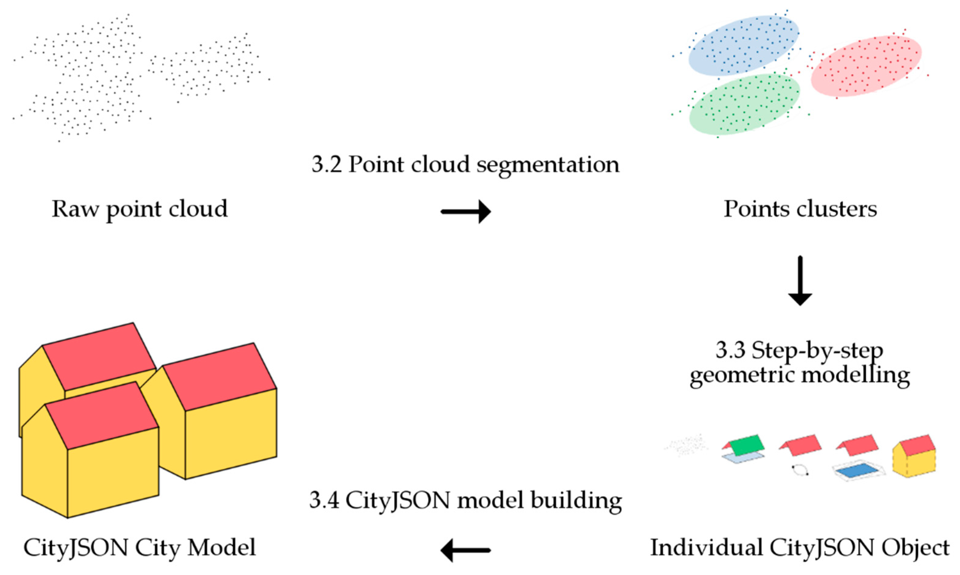
Figure 2.
ALS noise in roof formation.

Figure 3.
Point cloud segmentation workflow.

Figure 4.
Succession of the parts generation.
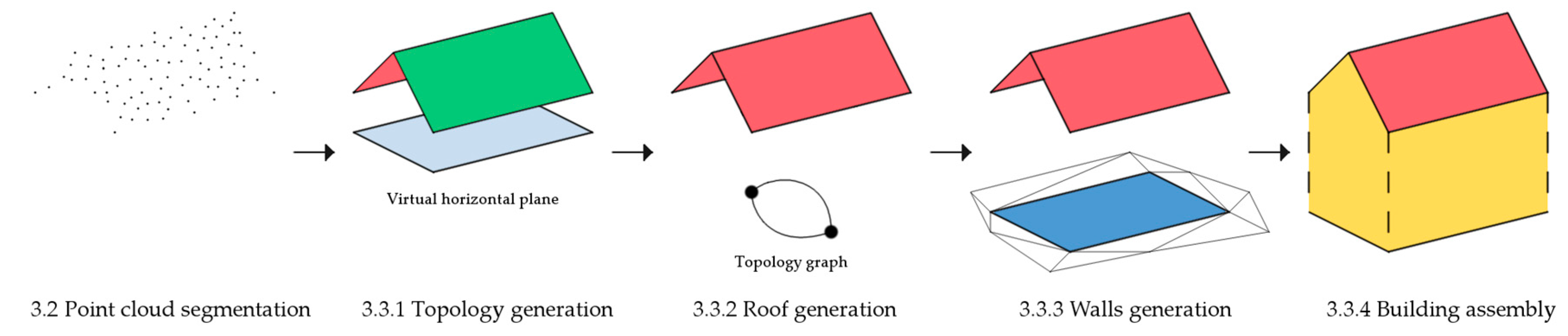
Figure 5.
Exploded reconstruction geometry following the modules.

Figure 6.
Relationships between slopes of adjacent planar-roof segments, based on Verma et al. 2006.
Figure 6.
Relationships between slopes of adjacent planar-roof segments, based on Verma et al. 2006.

Figure 7.
Representation of the roof skeleton in bold black.
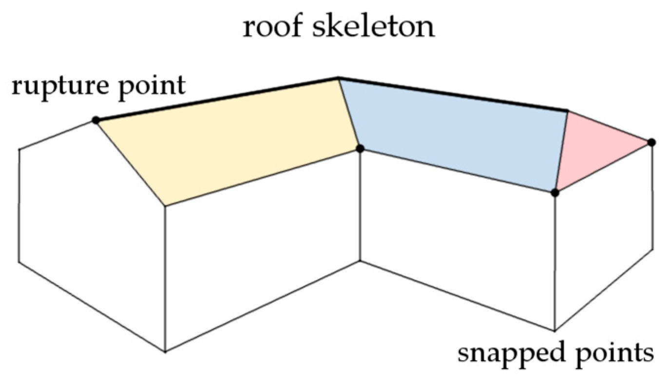
Figure 8.
Non-intersecting polygon construction.
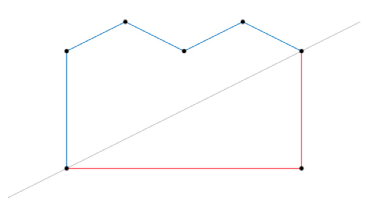
Figure 9.
Example of a geometry in which planes are not correctly oriented.
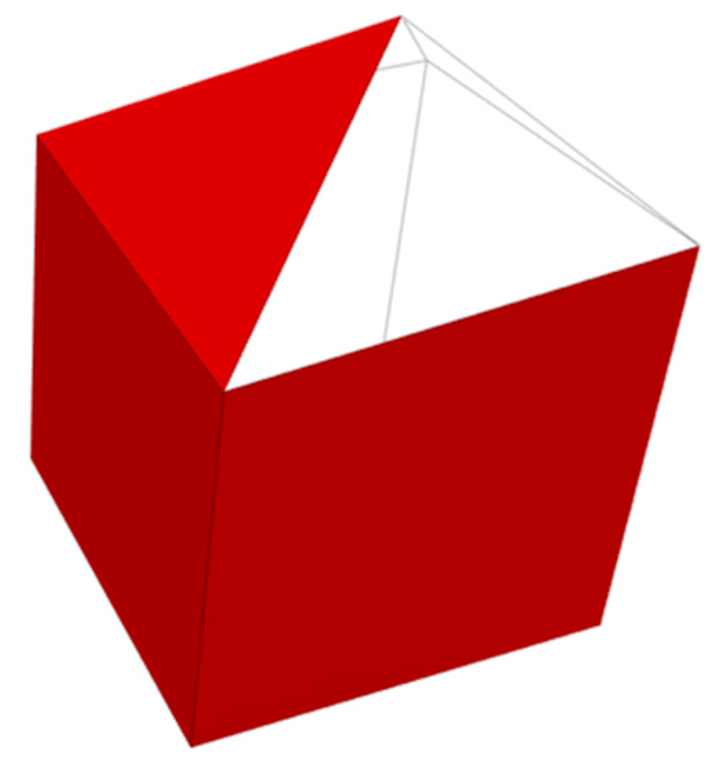
Figure 10.
Schema representation of the different levels of detail for the same building.

Figure 11.
Results from the city of Theux in CloudCompare and CityJSON viewers.

Figure 12.
From point clouds to building models.

Figure 13.
Translation from CityGML to CityJSON.
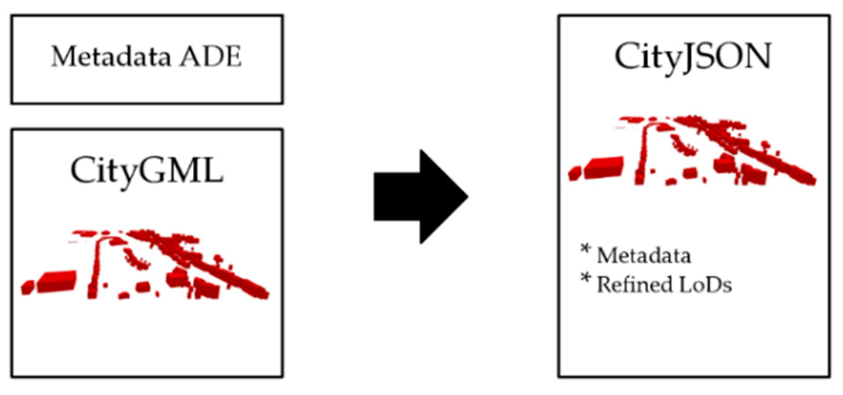
Figure 14.
Proportions of buildings reconstruction from Theux, Belgium.

Figure 15.
Number of planes par RMSE class.


Table 1.
Summarized comparison of results.
| City (Method) | Size | Buildings | Valid | Primitives | Valid |
|---|---|---|---|---|---|
| Berlin | 933 MB | 22.771 | 74% | 89.736 | 90% |
| DenHaag | 22 MB | 844 | 61% | 1.990 | 85% |
| Montréal | 125 MB | 581 | 76% | 1.744 | 88% |
| NRW | 16 MB | 797 | 83% | 928 | 77% |
| Theux (UR) | 689 KB | 420 | 92% | 1.198 | 97% |
| Theux (RG) | 656 KB | 400 | 93% | 1053 | 96% |
© 2020 by the authors. Licensee MDPI, Basel, Switzerland. This article is an open access article distributed under the terms and conditions of the Creative Commons Attribution (CC BY) license (http://creativecommons.org/licenses/by/4.0/).
Share and Cite
MDPI and ACS Style
Nys, G.-A.; Poux, F.; Billen, R. CityJSON Building Generation from Airborne LiDAR 3D Point Clouds. ISPRS Int. J. Geo-Inf. 2020, 9, 521. https://0-doi-org.brum.beds.ac.uk/10.3390/ijgi9090521
AMA Style
Nys G-A, Poux F, Billen R. CityJSON Building Generation from Airborne LiDAR 3D Point Clouds. ISPRS International Journal of Geo-Information. 2020; 9(9):521. https://0-doi-org.brum.beds.ac.uk/10.3390/ijgi9090521
Chicago/Turabian StyleNys, Gilles-Antoine, Florent Poux, and Roland Billen. 2020. "CityJSON Building Generation from Airborne LiDAR 3D Point Clouds" ISPRS International Journal of Geo-Information 9, no. 9: 521. https://0-doi-org.brum.beds.ac.uk/10.3390/ijgi9090521
Note that from the first issue of 2016, this journal uses article numbers instead of page numbers. See further details here.