Solar3D: An Open-Source Tool for Estimating Solar Radiation in Urban Environments


1
Zhejiang-CAS Application Center for Geoinformatics, Jiashan 314100, China
2
Aerospace Information Research Institute, Chinese Academy of Sciences, Beijing 100094, China
3
School of Environment and Planning, Liaocheng University, Liaocheng 252059, China
*
Author to whom correspondence should be addressed.
ISPRS Int. J. Geo-Inf. 2020, 9(9), 524; https://0-doi-org.brum.beds.ac.uk/10.3390/ijgi9090524
Submission received: 11 August 2020
/
Revised: 25 August 2020
/
Accepted: 29 August 2020
/
Published: 1 September 2020
(This article belongs to the Special Issue Virtual 3D City Models)
Abstract
:Solar3D is an open-source software application designed to interactively calculate solar irradiation on three-dimensional (3D) surfaces in a virtual environment constructed with combinations of 3D-city models, digital elevation models (DEMs), digital surface models (DSMs) and feature layers. The GRASS GIS r.sun solar radiation model computes solar irradiation based on two-dimensional (2D) raster maps for a given day, latitude, surface and atmospheric conditions. With the increasing availability of 3D-city models and demand for solar energy, there is an urgent need for better tools to computes solar radiation directly with 3D-city models. Solar3D extends the GRASS GIS r.sun model from 2D to 3D by feeding the model with input, including surface slope, aspect and time-resolved shading, which is derived directly from the 3D scene using computer graphics techniques. To summarize, Solar3D offers several new features that—as a whole—distinguish this novel approach from existing 3D solar irradiation tools in the following ways. (1) Solar3D can consume massive heterogeneous 3D-city models, including massive 3D-city models such as oblique airborne photogrammetry-based 3D-city models (OAP3Ds or integrated meshes); (2) Solar3D can perform near real-time pointwise calculation for duration from daily to annual; (3) Solar3D can integrate and interactively explore large-scale heterogeneous geospatial data; (4) Solar3D can calculate solar irradiation at arbitrary surface positions including on rooftops, facades and the ground.
1. Introduction
Solar radiation models are used to estimate solar energy that reaches the Earth’s surface. Traditional geographic information system (GIS)-based solar radiation models are designed primarily to obtain spatially and temporally resolved solar irradiation estimates on the ground over large geographic areas. With increasing demand for solar energy in urban areas—and increasing interest in researching urban climates at local scales—there has been an urgent need for better tools to estimate solar irradiation at local scales within urban areas. Traditional GIS solar radiation models, such as the widely used ESRI ArcGIS Solar Analyst (SA) [1] and GRASS GIS r.sun [2], can operate only on two-dimensional (2D) raster maps that supply the surface elevation. Moreover, in most cases, they cannot be used to estimate irradiation at vertical surfaces such as building facades. When modeling solar irradiation on the building scale, 2D raster maps are not able to represent complex geometric features such as vertical surfaces and overhangs, and the complexity of urban morphology can best be represented in three-dimensional (3D) city models in the form of triangular meshes. Owing to the advancements in unmanned aerial vehicle (UAV) and 3D-reconstruction technologies, oblique airborne photogrammetry-based 3D-city models (OAP3Ds or integrated meshes) have become widely available and are a valuable asset for solar energy assessment, energy planning and urban planning [3]. Despite this, little has been done to support the direct use of OAP3Ds in solar irradiation estimation. In summary, efforts are needed to develop an integrated solar radiation tool that overcomes these limitations so it can be applied to real-world scenarios more broadly.
A 3D-city model can be constructed in multiple ways, including by manually creating in computer-aided design (CAD) software, from LiDAR point clouds, from oblique airborne imagery and by extruding building footprints. Liang et al. [4] used graphics processing unit (GPU)-based ray casting to calculate solar irradiation on building roofs and facades, but the obtained solution was optimized specifically for building footprints-extruded 3D-city models and did not perform well with complex scenes comprising dense CAD meshes. Liang et al. [5] used a novel type of GPU ray casting technique accelerated with a sparse voxel octree to calculate solar irradiation on building surfaces in real time, but the solution cannot accommodate large scenes due to video memory limitation. Kaňuk et al. [6] recently developed a GRASS GIS r.sun extension to calculate solar irradiation on triangular irregular networks (TINs), which is a widely used GIS data format. By design, TINs are composed purely of contiguous, non-overlapping triangular facets. As such, they are essentially a 2.5D representation of the 3D world and therefore are subject to a loss of 3D geometric information.
The VI-Suite is a 3D environmental analysis toolset developed within the open-source CAD software Blender [7], and it was designed to interactively calculate and visualize solar irradiation on building surfaces. Although the VI-Suite allows users to import georeferenced raster maps as meshes into Blender, it loads all meshes at once into memory, and, thus may not be able to manage large-scale 3D-city models such as OAP3Ds. Robledo et al. [8] used GPU shadow mapping on WebGL to evaluate shading losses as a way to estimate solar irradiation on photovoltaic (PV) arrays. Shadow mapping proved to be a computationally efficient solution for computing solar radiation with 3D models, but it is susceptible to resampling errors [9] especially when the sun forms a narrow angle with the surface.
A common shortcoming of existing 3D-solar-radiation tools is a lack of support for interactive computation with large-scale level-of-detail (LOD) 3D-city models such as OAP3Ds. OAP3Ds distinguish itself from traditional 3D-model sources with its very high level of geometric accuracy and textural fidelity. Due to a lack of support for large-scale 3D-city models, when utilizing OAP3Ds in conventional solar radiation tools, they must be rasterized into digital surface models (DSMs) so that the solar tools can consume, and this 3D–2D conversion will result in information loss and geometric errors which will further propagates through the solar modeling process. Ideally, OAP3Ds should be utilized in their native form in solar radiation tools.
Additionally, although several 3D-solar-radiation tools that can work directly with 3D models have been developed, most of them are implemented in an isolated environment for use with a specific 3D-model format. Moreover, few of them support integration with other common geospatial data sources, such as digital elevation models (DEMs), DSMs and feature layers, which are essential background information needed for decision making in urban and energy planning [10].
Bearing in mind the above limitations, we developed a new solar irradiation tool designed specifically to meet the following requirements. (1) to support pointwise calculation of daily to annual irradiation at arbitrary surfaces including at rooftops, facades and the ground; (2) to provide near real-time computation and feedback; (3) support for interactive exploration and calculation; (4) to support heterogeneous 3D-model formats, including common CAD model formats, OAP3Ds and building footprint extrusions; and (5) to support the mash-up of local- to global-scale geospatial data sources, including DEMs, DSMs, imagery and feature layers with 2D and 3D symbology.
2. Methods
This section is divided into two parts. The first part introduces the r.sun solar radiation model and then delves into the conceptualization and key technologies of the 3D extension. The second part is focused on the software architecture and business logic of Solar3D.
2.1. The Solar Radiation Model
The r.sun model breaks the global solar radiation into three components: the beam (direct) radiation, the diffuse radiation and the reflective radiation [2]. The beam irradiation is usually the largest component and the only one that accounts for direct shadowing effect, which is a major factor determining the accessibility of solar energy in urban environments. The clear sky beam irradiance on a horizontal surface Bhc [W.m-2], which is the solar energy that traverses the atmosphere to reach a horizontal surface, is derived using the following Equation (1) [2]:
where TLK, G0, m and δR(m) are, respectively the air mass Linke turbidity factor, the extraterrestrial irradiance normal to the solar beam, the solar altitude and the Rayleigh optical thickness, and Bhc is converted into the clear sky beam irradiance on an inclined surface Bic [W.m-2] using the following Equation (2) [2]:
where Mshadow is the shadowing effect determined by the solar vector Vsun and the shadow casting objects in the scene. The solar vector Vsun is determined by the solar azimuth angle (θ) and the solar altitude angle (φ). δexp is the solar incidence angle measured between the sun and an inclined surface described by the slope and aspect angle. Mshadow a binary shadow mask which returns 0 when the direct-beam light of the sun is blocked or otherwise returns 1. When applying the r.sun model to 3D-city models instead of 2D raster maps, a major technical challenge is to calculate the shadow mask accurately and rapidly for each time step.
Ray casting is a conventional and accurate shading evaluation method [4]. When performing ray casting, a ray oriented in the target direction is cast to intersect with all triangles in the 3D scene; therefore, this method is computationally intensive. Computation performance is especially critical for calculating long-duration irradiation with high temporal resolution. For example, when calculating annual solar irradiation with a temporal resolution of 10 min, a total of 8760 × 6 rays need to be cast for the shading for each time step to be evaluated and, moreover, the time cost of casting a ray is directly correlated with the geometric complexity of the scene.
An alternative approach to evaluate shading is to produce a shadow map from the solar position for each time step [8]. Shadow mapping can be easily implemented on the GPU to provide real-time rendering. However, shadow mapping is susceptible to various quality issues associated with perspective aliasing, projective aliasing and insufficient depth precision [9]. Moreover, when performing time-resolved shading evaluation with shadow maps for a specific location, the shadow mask of each time step needs to be evaluated at a different image-space location on a separate shadow map. Therefore, the results could be subject to notable spatiotemporal uncertainty.
Hemispherical photography is another approach to evaluating shading and estimating solar irradiation [11]. In hemispherical photography, a fisheye camera with a 360-degree horizontal view and a 180-degree vertical view is placed at the ground looking upward, producing a hemispherical photograph in which all sky directions are simultaneously visible. As the visibility in all sky directions are preserved in the resulting hemispherical photograph, it can be used to determine if the direct beam of the sun is obstructed for any given time of the year.
One of the goals of Solar3D is to provide accurate pointwise estimates of hourly to annual irradiation with high temporal resolution. Having reviewed the three main shading evaluation techniques with this goal in mind, we endeavored to follow the hemispherical photography approach based on the following considerations. (1) In terms of geometric accuracy and uncertainty, given a sufficient image resolution, it is theoretically nearly as accurate as ray casting, and it is not subject to the notable spatiotemporal uncertainty that is associated with shadow mapping; (2) In terms of computation efficiency, theoretically, it scales better with geometric complexity than ray casting; therefore, it can compute faster with 3D-city models, which typically have very high geometric complexity. Furthermore, although shadow mapping may be faster in areal computation, we are focused on accurate pointwise computation; therefore, sacrificing accuracy for performance is not an ideal option.
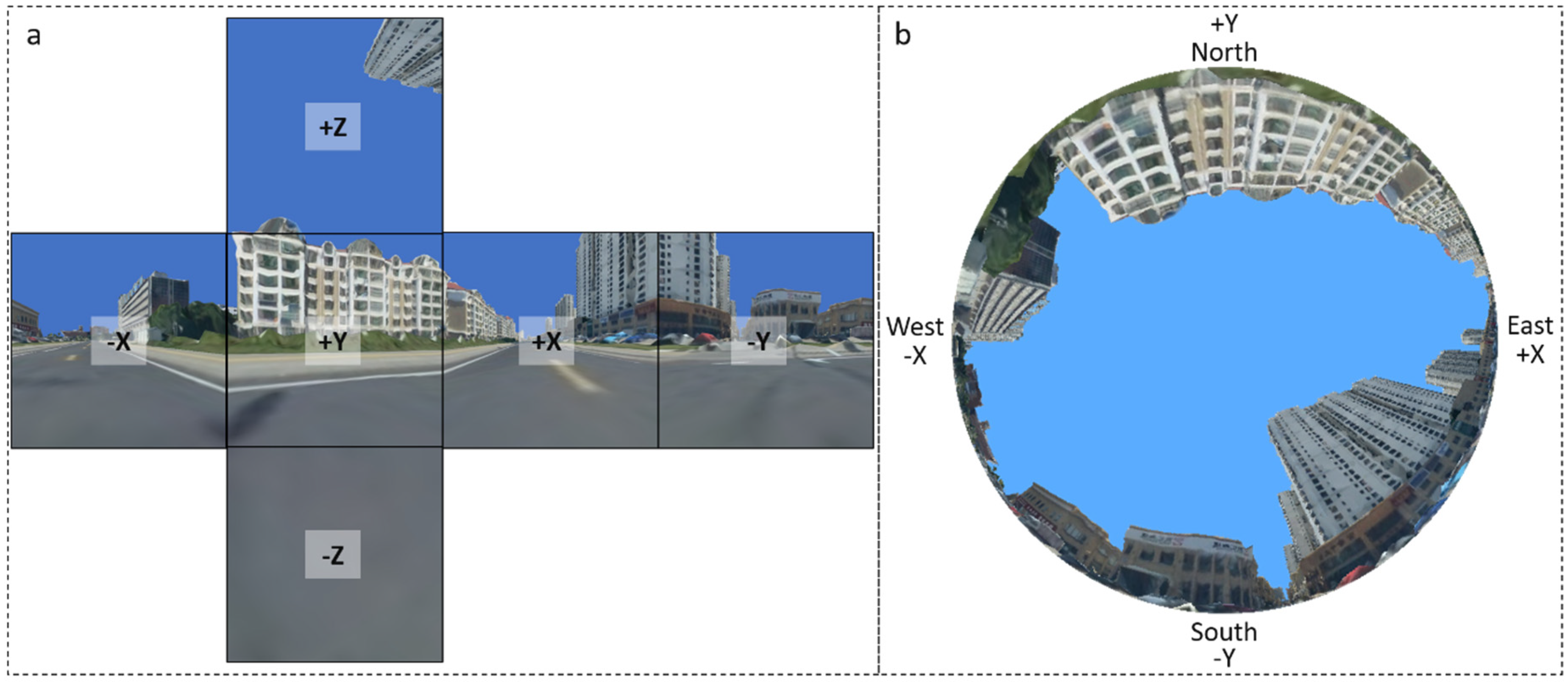
A hemispherical photograph is essentially a 3D panorama projected onto a circle in a 2D image (Figure 1b). A hemispherical projection can result in oversampling, under-stamping and image distortion. To avoid these issues, instead of relying directly on a projected hemispherical photograph for shading evaluation, we use a 360-panoram in its native form.
In computer graphics, cube mapping is a common technique that is used to preserve a 360-degree panoramic snapshot of the surrounding environment at a given location [12]. A cube map (Figure 1a) is composed of six images facing north (positive Y), south (negative Y), east (positive X), west (negative X), the sky (positive Z) and the ground (negative Z). To generate a cube map of a scene, the scene needs to be rendered once for each of the cube’s face. We use OpenGL and the GLSL shading language to generate a cube map as follows [13]:
- (1)
- Allocate a render target texture (RTT) with an alpha channel for each cube map face;
- (2)
- Construct a camera with a 90-degree horizontal and vertical view angle at the given location in the scene;
- (3)
- For each of the six cube map faces, set up the camera so it is aligned in the direction of the cube map face and initialize the RRT with a transparent background (alpha = 0) and then render the scene offscreen to the associated RTT. The scene must be set up so that it is not enclosed or obstructed by any objects that are not part of the scene, for example by a sky box, so that only the potential shadow-casting objects in the scene will pass the z-buffering test and be shaded with nonzero alpha values. Hence, in the resulting cube map face images, the sky and non-sky pixels can be distinguished by their respective alpha mask values.
At this stage, the shadow mask needed for each time step for use in Equation (2) can be easily determined by looking up the classified cube map image pixels. When looking up a cube map to access the pixel for a given solar position in spherical coordinates , the following steps are performed:
- (1)
- Determine the cube map face to look up. As all six cube map faces have a 90-degree horizontal and vertical view angle, the cube map face index can be determined using the solar position (θ, φ) by following the logic expressed in Equation (3):
- (2)
- Project the solar position into the image space and fetch the pixel at the resulting image coordinates. The image-space coordinates are obtained using Equation (4):
Finally, in addition to the shadow masks, to calculate the irradiation on an inclined surface in a 3D-city model using r.sun, the remaining information needed by r.sun includes the slope and aspect of the surface, which can be easily derived from the surface normal vector [4].
2.2. The Computation and Software Framework
The core framework is constructed by integrating the r.sun solar radiation model into a 3D-graphics engine, OpenSceneGraph [14], an OpenGL-based 3D-graphics toolkit widely used in visualization and simulation. OpenSceneGraph is essentially an OpenGL state manager with extended support for scene graph and data management. The source code of the r.sun model was detached from the GRASS GIS repository and integrated into the Solar3D codebase, and it was modified so that the r.sun model can be programmatically called to calculate irradiation with custom parameters. The reasons for choosing OpenSceneGraph are multifold: first, OpenSceneGraph provides user-friendly, object-oriented access to OpenGL interfaces; second, OpenSceneGraph provides built-in support for interactive rendering and loading of a wide variety of common 3D-model formats including osg, ive, 3ds, dae, obj, x, fbx and flt; third, OpenSceneGraph supports smooth loading and rendering of massive OAP3Ds, which are already being widely used in urban and energy planning. Once exported from image-based 3D-reconstruction tools such as Esri Drone2Map and Skyline PhotoMesh into OpenSceneGraph’s Paged LOD format, OAP3Ds can be rapidly loaded into OpenSceneGraph for view-dependent data streaming and rendering. The r.sun model in Solar3D also relies on OpenSceneGraph for supplying the key parameters needed for irradiation calculation. (1) location identified at a 3D surface; (2) slope and aspect angles of the surface; (3) time-resolved shadow masks evaluated from a cube map rendered at the identified position.
OpenSceneGraph, as the rendering engine in Solar3D, serves several purposes. (1) it is used to render 3D-city models that come in different formats, including OAP3Ds, CAD models and procedurally generated 3D models such as those extruded from building footprints; (2) it is used to render the scene into cube maps for shading evaluation; (3) it renders the UI that gathers user input and provides feedback; (4) it handles user device input, primarily moue actions, so that users can interact with the UI and the 3D scene.
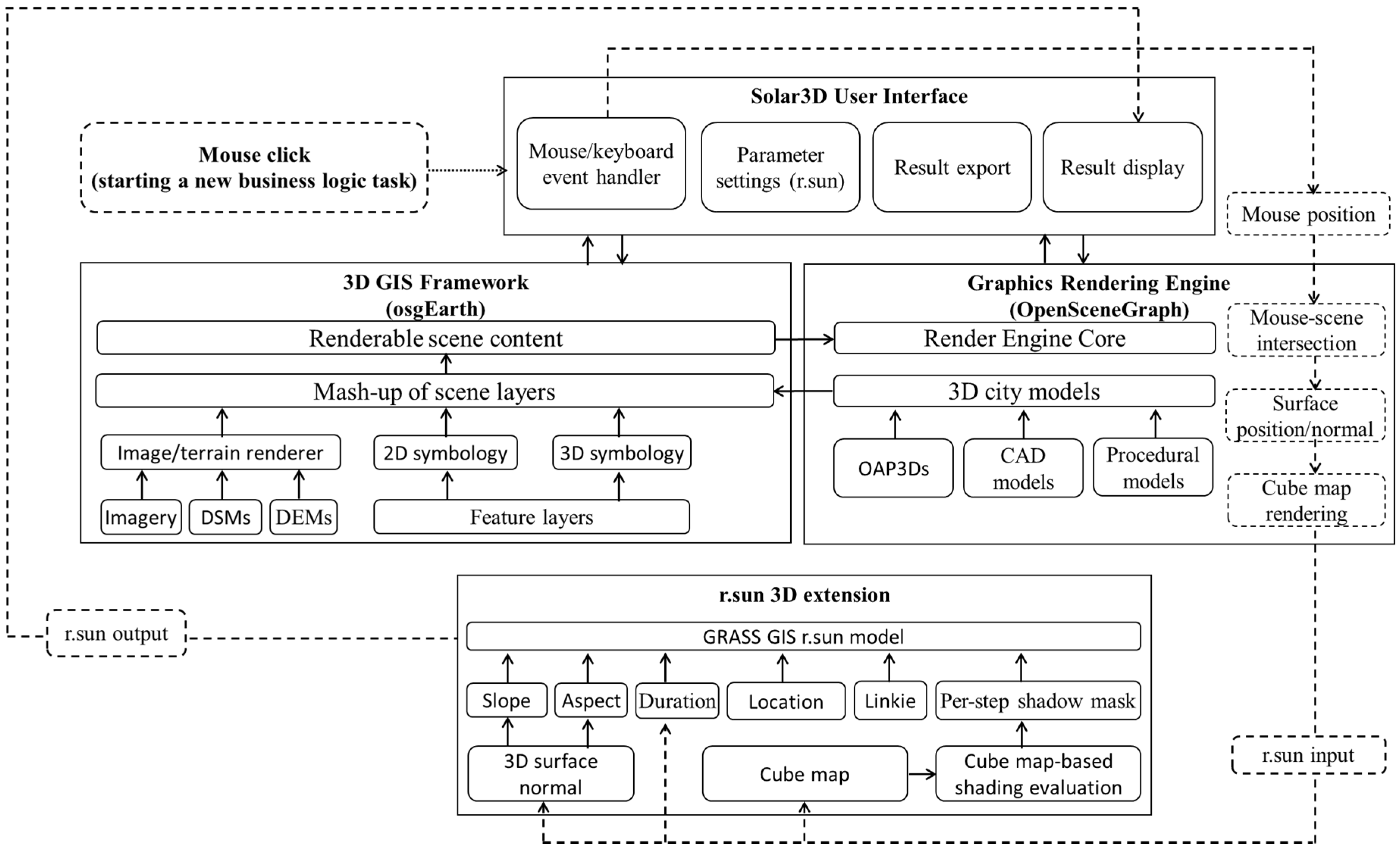
The business logic of the core framework works in a loop triggered by user requests (Figure 2): (1) a user request is started by mouse-clicking at an exposed surface in a 3D scene rendered in an OpenSceneGraph view overlaid with the Solar3D user interface (UI) elements; (2) the 3D position, slope and aspect angle are derived from the clicked surface; (3) a cube map is rendered at the 3D position as described above; (4) all required model input [15], including the geographic location (latitude, longitude, elevation), Linkie turbidity factor, duration (start day and end day), temporal resolution (in decimal hours), slope, aspect and shadow masks for each time step, is gathered, compiled and fed to r.sun for calculating irradiation. The shadow masks are obtained by sampling the cube map with the solar altitude and azimuth angle for each time step; (5) the r.sun model is run with the supplied input to generate the global, beam, diffuse and reflective irradiation values for the given location; (6) the r.sun-generated irradiation results are returned to the Solar3D UI for immediate display.
To better facilitate urban and energy planning, the core framework is further extended by integrating into a 3D-GIS framework (Figure 2), osgEarth [16], an OpenSceneGraph-based 3D geospatial library used to author and render planetary- to local-scale 3D GIS scenes with support for most common GIS content formats, including DSMs, DSMs, local imagery, web map services, web feature service and Esri Shapefile. With the 3D GIS extension, Solar3D can serve more specialized and advanced user needs, including. (1) hosting multiple 3D-city models distributed over a large geographic region; (2) overlaying 3D-city models on top of custom basemaps to provide an enriched geographic context in support of energy analysis and decision making; (3) incorporating the topography surrounding a 3D-city model into shading evaluation; (4) interactively calculating solar irradiation with only DSMs.
Users can start OAP3D with an osgEarth scene by providing a xml configuration file (.earth) authored following osgEarth’s scene authoring specifications. An osgEarth scene (.earth) starts with a map node. A map can be created either as a global or a local scene by specifying the type attribute (type = “geocentric” for a global scene or type = “projected” for a local scene) in the map node. Under the map node, users can add different layer nodes, including image layers, feature layers, elevation layers, model layers and annotations. A layer node is created by providing the layer type, data source and other data symbology and rendering attributes. For example, an image layer can be added by providing the driver attribute (TMS, GDAL, WMS, ArcGIS) and URL attribute (e.g., http://readymap.org/readymap/tiles/1.0.0/22/).
The code was written in C++ and complied in Visual Studio 2019 on Windows 10. The three main dependent libraries used, OpenSceneGraph, osgEarth and Qt5, were all pulled from vcpkg [17], a C++ package manager for Windows, Linux and MacOS, and therefore Solar3D can potentially be complied on Linux and MacOS with additional work to set up the build environment. Solar3D is publicly available at https://github.com/jian9695/Solar3D.
3. Results
The discussion of the results begins with an evaluation of Solar3D. The evaluation was designed with two questions in mind. The first question is ‘How reliable is the cube map-based shading evaluation technique and how does cube map size affect shading accuracy?’ As the accuracy of the beam irradiation is largely dependent on the shading evaluation algorithm, it is of critical importance to have a quantitative understanding of the cube map-based shading evaluation technique. The second question is ‘how does the extended 3D r.sun, i.e., Solar3D, perform in complex urban environments in comparison to the original 2D r.sun?’ The remainder of this section is dedicated to demonstrating the general business workflow and main features of Solar3D.
3.1. Evaluation of the Cube Map-based Shading Technique
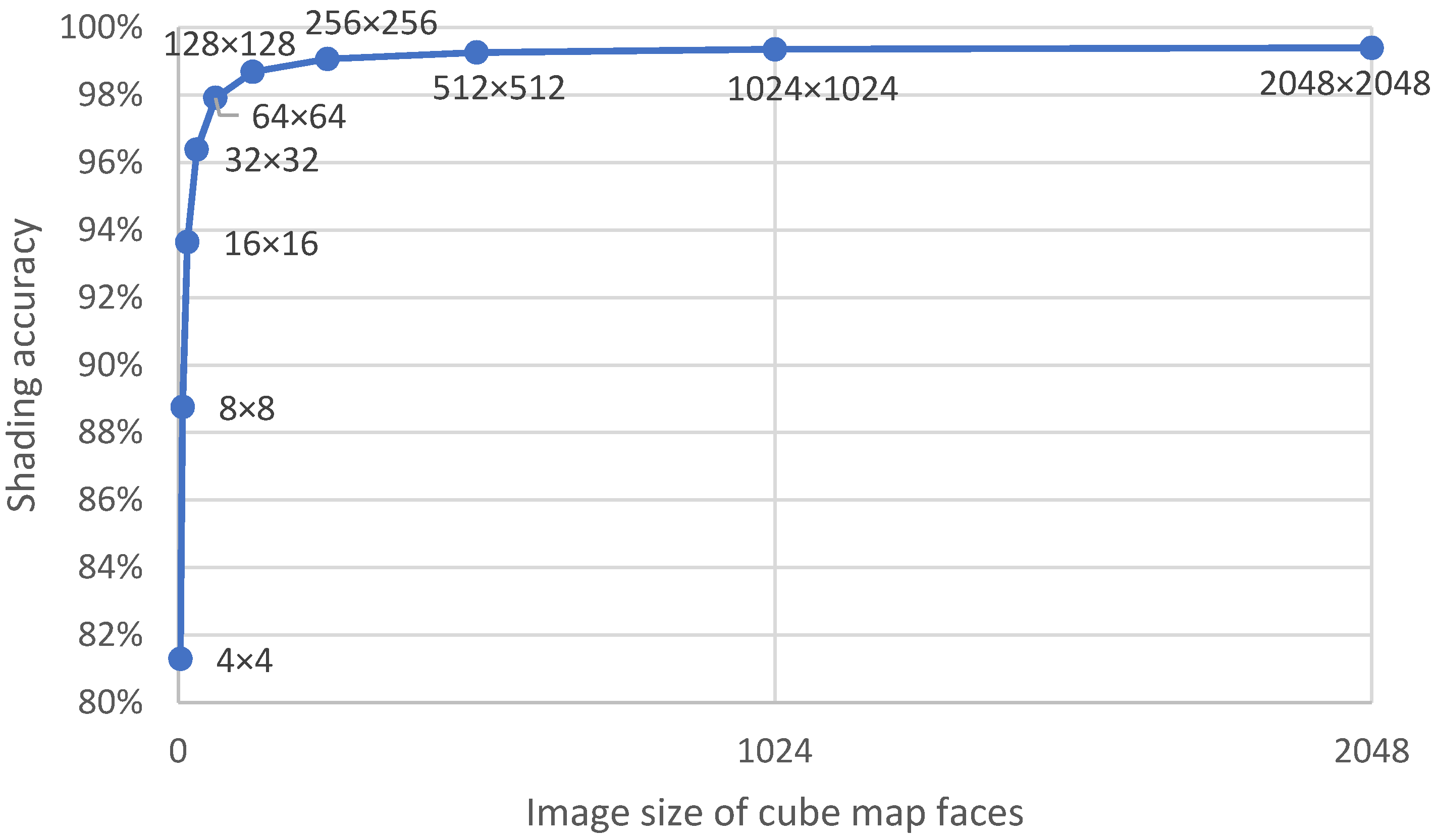
Theoretically, the accuracy of the cube map-based shading technique is determined by the size of the cube map—or more specifically—by the image size of the six cube map faces. To quantify how the shading accuracy correlates with the cube map size, we performed a comparison of the cube map-based shading technique against the rigorous ray-casting algorithm with cube map (face) sizes ranging from 4 × 4 pixels to 2048 × 2048 pixels including all powers of two in between.
The 3D-city model used for the comparison is an OAP3D that covers a 45 km2 downtown area of the coastal city Weihai, China located at 37.5131° N, 122.1204° E. The OAP3D was captured using a quadcopter with an image resolution of approximately 10–20 cm and generated using Skyline Photomesh.
The comparison was made within a 1 km2 area. First, a total of 1000 locations were randomly generated within the defined area. Then, cube maps from 4 × 4 to 2048 × 2048 pixels were generated at each of these sample locations. After this, shading was evaluated using both methods at sky directions regularly spaced at 5 degrees with solar altitude angles ranging from 0–90 and azimuth angles ranging from 0–360. Finally, for each of the sample locations, we calculated the percentage of the sky directions at which the cube map technique gives a correct result (shaded or not) as compared against ray casting. The average percentage of all sample locations is used as a measure of shading accuracy.
The comparison shows a nonlinear relationship between the image size of cube map faces and the accuracy of the cube map-based shading technique (Figure 3). When the image size is in the lower range, a small increase results in a larger improvement in shading accuracy. Specifically, when the image size is increased from 4 × 4 to 128 × 128, the shading accuracy is significantly improved from 81.28% to 98.69%. However, when the image size is larger than 128 × 128, further increase in image size results in a very small improvement in accuracy. As Figure 1 shows, when the image size is increased from 256 × 256 to 2048 × 2048, the shading accuracy is improved only slightly, from 99.07% to 99.40%. This suggest that when the image size of the cube map faces is set to be equal or larger than 256 × 256, the cube map-based shading technique should be able to perform at a higher than 99% accuracy.
3.2. Comparison of the 3D Extension with the Original r.sun 2D
The objective of the comparison is to determine the differences in clear-sky irradiation estimates between the 3D extension and the original r.sun 2D when both are applied in a complex urban environment. For the 3D-city model to be consumed in the original r.sun 2D, we converted the 3D meshes into a DSM regularly gridded at 0.25 m, and the conversion was performed using a computer graphics approach by rendering the height attribute of the 3D meshes into a 4000 × 4000 image.
The data used for the comparison is the same 1 km-by-1 km area as described in Section 3.1. The comparison was performed for three different lengths of duration, including daily (Day 1), monthly (Days 1–31) and annually (Days 1–365), for 1000 randomly generated locations within the defined area, and the time step and Linke turbidity factor were set at 0.5 h and 3.0, respectively.
Presumably, the differences in clear-sky irradiation estimates between the 3D extension and the original r.sun can arise from several sources, such as the following. (1) differences in surface orientation (slope and aspect) caused by the difference in data representation (3D mesh versus 2D raster); (2) differences in the distribution of the sky areas being blocked due to the difference in data representation; and (3) difference in shading evaluation methodology (computer graphics-based cube map versus raster-based analytical visibility algorithm). As a DSM is a rasterized representation of 3D surfaces and the rasterization of meshes is known to be subject to a loss of geometric information, we are inclined to exclude the effect of surface orientation on the differences between irradiation estimates. With this rationale in mind, when generating the random locations, we discarded those where the surface slope is greater than 5 degrees and continued until 1000 qualified locations were collected.
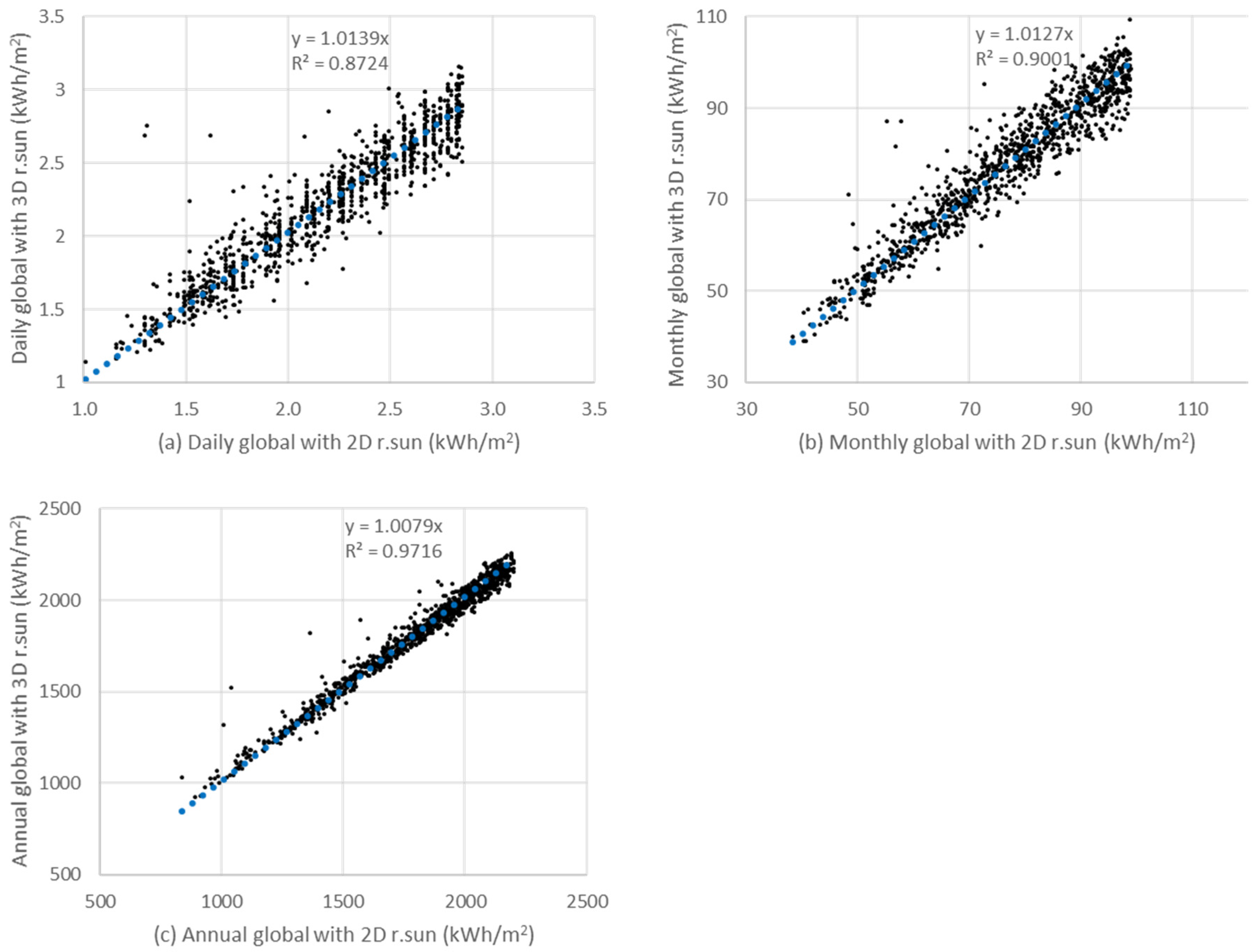
The comparison (Figure 4) shows that overall, the global irradiation estimates produced by the r.sun 3D extension closely correlate with those produced by the original r.sun with R-squared values ranging from 0.87 to 0.97. The comparison also shows that the 3D estimates tend to correlate better with the 2D estimates for a longer duration. This implies an overall agreement in the percentage of obstructed sky directions (obstructed sky directions divided by total sky directions) especially in the case of annual duration in which the entire sky dome was considered.
3.3. Basic Usage and Workflow
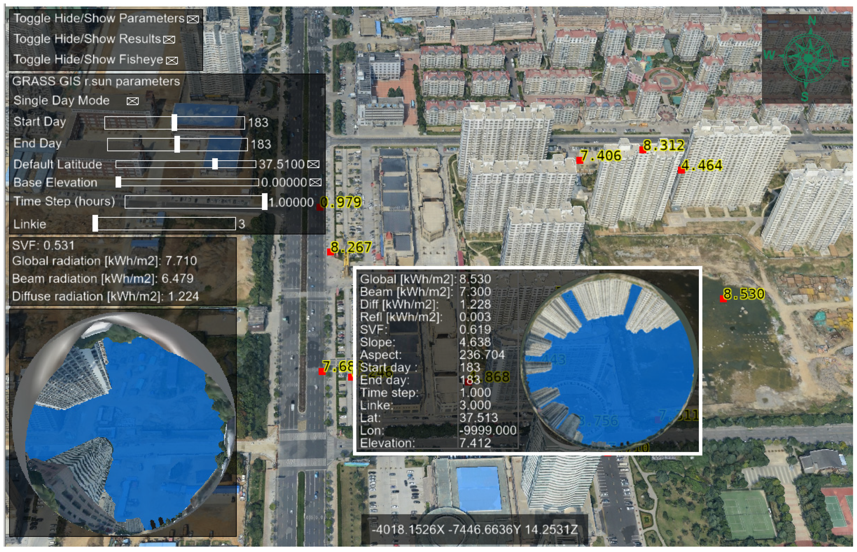
The Solar3D UI consists of three components, respectively responsible for the parameter settings, the results display and status updates. The parameter settings panels are located on the top left with UI elements for setting the Linke factor, start day, end day, time step, latitude and base elevation overrides (used in case of a non- georeferenced scene). The result display UI consists of two panels located on the left side right below the parameter settings panel used for immediate display of feedback from the latest request and a popup panel used to display results at the cursor point. The status UI elements include a compass at the top right and a status bar displaying cursor and camera coordinates toward the bottom.
One of the first steps in the workflow of Solar3D is scene preparation. Users are expected to prepare scenes with a least one 3D model and (optionally) some basemaps. An easy way to use Solar3D is to start the program with the path of a single 3D model exported from CAD or an OAP3D exported from photo-based 3D reconstruction software (Figure 5), but started this way, the scene will not be georeferenced, and, thus, the users will need to specify the latitude and base elevation override.
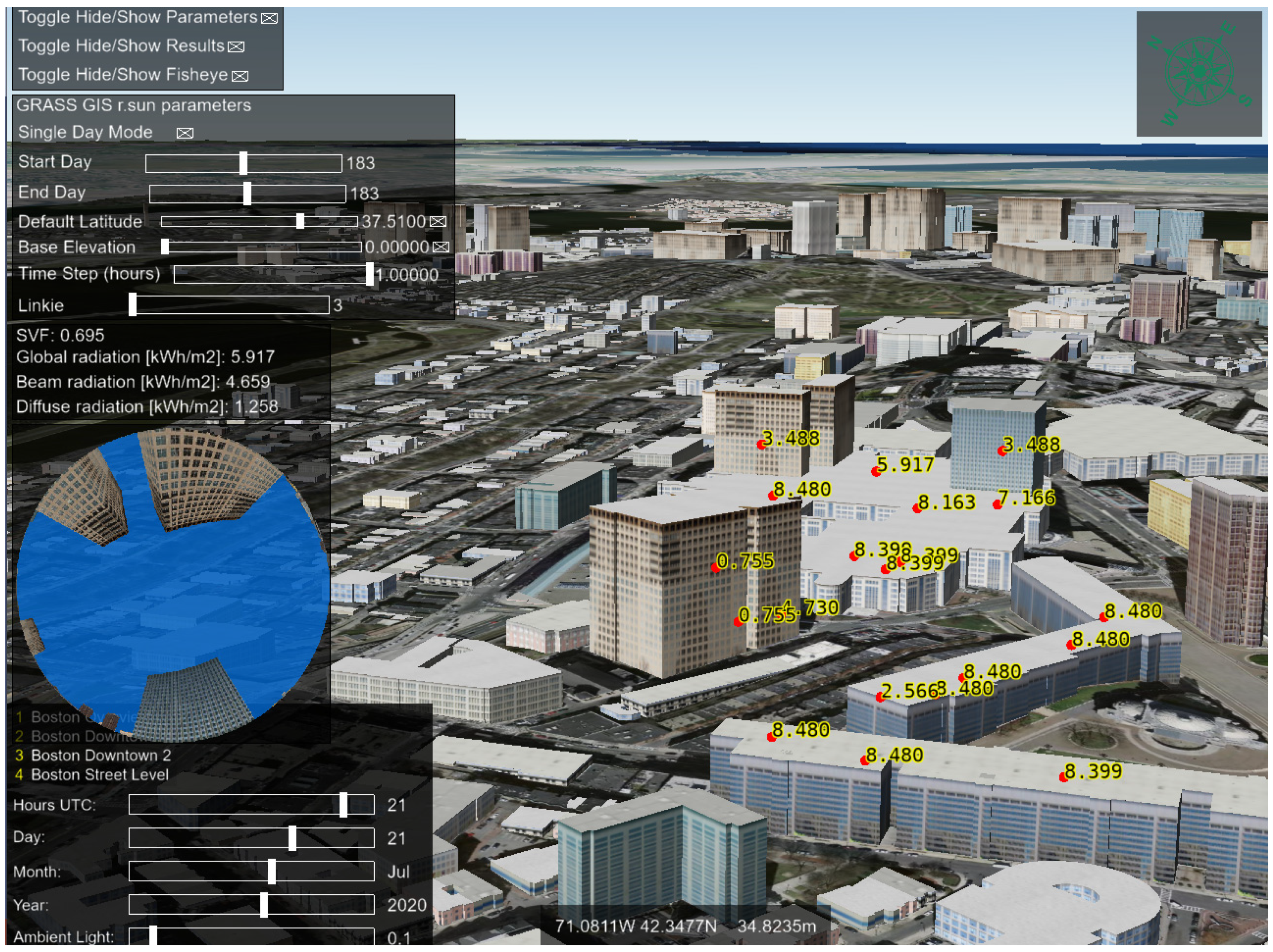
To integrate 3D models into a georeferenced scene with basemaps (Figure 6), users need to follow the instructions and examples provided by osgEarth [16]. One inconvenience of this method is that osgEarth does not offer a scene editor with a graphic UI for scene authoring. Instead, users need to manually add and configure scene layers in a text editor based on one of the example configuration files (*.earth). An advantage with osgEarth is it that can be used to author advanced scenes with 3D models overlaid on DEMs and DSMs distributed all over the Earth. Additionally, osgEarth provides the ability to extrude building footprints from polygon features into 3D models for use in Solar3D.
In a typical use scenario, after starting Solar3D with a single 3D model or an osgEarth scene, the user zooms into an area of interest with buildings on which PV arrays are planned to be deployed. Then, irradiation estimates are obtained by interactively clicking at rooftops and facades to identify suitable surface areas for PV deployment. Solar3D processes calculation requests, upon the click of a mouse (with the Ctrl key on the keyboard held down) once at a time. The program typically finishes a request within a couple of seconds and displays the results immediately. A marker with a text label is displayed at the location where the calculation request was finished. The irradiation results obtained during a session can be exported in a batch to a comma-delimited text file for analysis. When exporting an irradiation record, the associated r.sun parameters and 3D coordinates are packed into a single row. For further details, refer to the source code [18], user guide [19] and demonstration video [20].
4. Discussion and Conclusions
Solar3D was developed using a mature graphics rendering engine (OpenSceneGraph) and a full-featured 3D-GIS framework (osgEarth), as a 3D extension of the GRASS GIS r.sun model. Solar3D relies on a cube map-based computer graphics technique to calculate pointwise solar irradiation in near real time for up to a year. OpenSceneGraph enables Solar3D to effectively consume massive 3D-city models in heterogeneous forms, including OAP3Ds, CAD models and building footprint extrusions. Moreover, osgEarth enables Solar3D to consume large-scale geospatial data in the forms of DSMs, DEMs, imagery and feature layers, which can serve not only as geometric data for shading evaluation, but also as integrated and informative geographic background to assist energy-related decision making.
Solar3D was evaluated mainly on two aspects: the accuracy of the cube map-based shading evaluation technique and its agreement with the original 2D r.sun. When compared against the rigorous ray-casting algorithm, the cube map-based shading evaluation technique achieved a 99% accuracy as long as all six cube map faces were allocated to an image size of at least 256 × 256 pixels. When compared with the original 2D r.sun, Solar3D shows an overall agreement in its global irradiation estimates. The correlation tends to be higher for longer duration as suggested by the increasing R-squared values of 0.87, 0.90 and 0.97 for daily, monthly and annual global irradiation estimates, respectively.
To conclude, Solar3D offers several new features that, as a whole, distinguish this novel approach from existing 3D solar irradiation tools in the following ways. (1) Solar3D can consume-to-consume massive heterogeneous 3D-city models; (2) Solar3D can perform near real-time pointwise calculation for duration from daily to annual; (3) Solar3D can integrate and interactively explore large-scale heterogeneous geospatial data; (4) Solar3D can calculate solar irradiation at arbitrary surface positions including on rooftops, facades, the ground, under a canopy or in the mountains.
Solar3D, in its current form, is subject to several limitations: first, it cannot be used to perform areal calculation which is an important utility in solar energy assessment. Although Solar3D can theoretically be extended to perform areal calculation, computation performance could become a concern when large areas are being considered and a potential solution is to accelerate shading evaluation using alternative approaches such as shadow mapping; Second, as a simple extension of a 2D solar radiation model, Solar3D has not considered many complex factors that may affect light propagation in urban environments and these include reflective materials, plant canopies and multiple scattering.
Author Contributions
Conceptualization, Jianming Liang; Data curation, Jianhua Gong; Investigation, Xiuping Xie and Jun Sun; Methodology, Jianming Liang; Project administration, Jianhua Gong; Software, Jianming Liang; Writing—original draft, Jianming Liang; Writing—review & editing, Jianhua Gong, Xiuping Xie and Jun Sun; All authors reviewed and edited the manuscript. All authors have read and agreed to the published version of the manuscript.
Funding
This research was supported by the National Natural Science Foundation of China (grant 41701469); The Strategic Priority Research Program of the Chinese Academy of Sciences (grant XDA19090114); The CAS Zhejiang Institute of Advanced Technology Fund (grant ZK-CX-2018-04); The Jiashan Science and Technology Plan Project (grant 2018A08).
Conflicts of Interest
The authors declare no conflict of interest.
References
- Fu, P.; Rich, P.M. A geometric solar radiation model with applications in agriculture and forestry. Comput. Electron. Agric. 2003, 37, 25–35. [Google Scholar] [CrossRef]
- Hofierka, J.; Súri, M. The solar radiation model for Open source GIS: Implementation and applications. In Proceedings of the Open Source GIS-GRASS Users Conference, Trento, Italy, 11–13 September 2002. [Google Scholar]
- Liang, J.; Shen, S.; Gong, J.; Liu, J.; Zhang, J. Embedding user-generated content into oblique airborne photogrammetry-based 3D city model. Int. J. Geogr. Inf. Sci. 2017, 31, 1–16. [Google Scholar] [CrossRef]
- Liang, J.; Gong, J.; Li, W.; Ibrahim, A.N. A visualization-oriented 3D method for efficient computation of urban solar radiation based on 3D-2D surface mapping. Int. J. Geogr. Inf. Sci. 2014, 28, 780–798. [Google Scholar] [CrossRef]
- Liang, J.; Gong, J. A sparse voxel octree-based framework for computing solar radiation using 3d city models. ISPRS Int. J. Geo Inf. 2017, 6, 106. [Google Scholar] [CrossRef] [Green Version]
- Kanuk, J.; Zubal, S.; Šupinský, J.; Šašak, J.; Bombara, M.; Sedlák, V.; Gallay, M.; Hofierka, J.; Onacillová, K. Testing of V3.sun module prototype for solar radiation modelling on 3D objects with complex geometric structure. Int. Arch. Photogramm. Remote Sens. Spat. Inf. Sci. ISPRS Arch. 2019, 42, 35–40. [Google Scholar] [CrossRef] [Green Version]
- Southall, R.; Biljecki, F. The VI-Suite: A set of environmental analysis tools with geospatial data applications. Open Geospatial Data Softw. Stand. 2017, 2, 23. [Google Scholar] [CrossRef]
- Robledo, J.; Leloux, J.; Lorenzo, E.; Gueymard, C.A. From video games to solar energy: 3D shading simulation for PV using GPU. Sol. Energy 2019, 193, 962–980. [Google Scholar] [CrossRef]
- Scherzer, D.; Wimmer, M.; Purgathofer, W. A survey of real-time hard shadow mapping methods. Comput. Graph. Forum 2011. [Google Scholar] [CrossRef] [Green Version]
- Resch, B.; Sagl, G.; Trnros, T.; Bachmaier, A.; Eggers, J.B.; Herkel, S.; Narmsara, S.; Gündra, H. GIS-based planning and modeling for renewable energy: Challenges and future research avenues. ISPRS Int. J. Geo Inf. 2014, 3, 662–692. [Google Scholar] [CrossRef]
- Gong, F.Y.; Zeng, Z.C.; Ng, E.; Norford, L.K. Spatiotemporal patterns of street-level solar radiation estimated using Google Street View in a high-density urban environment. Build. Environ. 2019, 148, 547–566. [Google Scholar] [CrossRef]
- Matzarakis, A.; Matuschek, O. Sky view factor as a parameter in applied climatology-Rapid estimation by the SkyHelios model. Meteorol. Z. 2011, 20, 39–45. [Google Scholar] [CrossRef]
- Liang, J.; Gong, J.; Sun, J.; Liu, J. A customizable framework for computing sky view factor from large-scale 3D city models. Energy Build. 2017, 149, 38–44. [Google Scholar] [CrossRef]
- OpenSceneGraph. Available online: http://www.openscenegraph.org (accessed on 14 July 2020).
- GRASS GIS r.sun. Available online: https://grass.osgeo.org/grass78/manuals/r.sun.html (accessed on 14 July 2020).
- osgEarth. Available online: http://osgearth.org (accessed on 14 July 2020).
- vcpkg. Available online: https://github.com/microsoft/vcpkg (accessed on 14 July 2020).
- Solar3D Source Code Repository. Available online: https://github.com/jian9695/Solar3D (accessed on 22 July 2020).
- Solar3D User Guide. Available online: https://github.com/jian9695/Solar3D/blob/master/User_Guide.pdf (accessed on 26 July 2020).
- Solar3D Demonstration Video. Available online: https://youtu.be/6zWNaCaH-RE (accessed on 22 July 2020).
Figure 1.
(a) Cube map and (b) hemispherical view at the same ground location.

Figure 2.
Solar3D architecture (solid boxes and arrows) and business logic (dashed boxes and arrows).
Figure 2.
Solar3D architecture (solid boxes and arrows) and business logic (dashed boxes and arrows).

Figure 3.
Shading accuracy of the cube map-based technique versus image size of cube map faces.

Figure 4.
Comparison of global solar irradiation estimates between the r.sun 3D extension and the original r.sun (2D) for different durations. (a) Daily (Day 1) global; (b) month (Days 1–31) global; (c) annual global (Days 1–365).
Figure 4.
Comparison of global solar irradiation estimates between the r.sun 3D extension and the original r.sun (2D) for different durations. (a) Daily (Day 1) global; (b) month (Days 1–31) global; (c) annual global (Days 1–365).

Figure 5.
Calculating solar irradiation with an OAP3D in Solar3D.

Figure 6.
Calculating solar irradiation with a building footprint-extruded 3D-city model (Boston) overlaid on a basemap in Solar3D.
Figure 6.
Calculating solar irradiation with a building footprint-extruded 3D-city model (Boston) overlaid on a basemap in Solar3D.

© 2020 by the authors. Licensee MDPI, Basel, Switzerland. This article is an open access article distributed under the terms and conditions of the Creative Commons Attribution (CC BY) license (http://creativecommons.org/licenses/by/4.0/).
Share and Cite
MDPI and ACS Style
Liang, J.; Gong, J.; Xie, X.; Sun, J. Solar3D: An Open-Source Tool for Estimating Solar Radiation in Urban Environments. ISPRS Int. J. Geo-Inf. 2020, 9, 524. https://0-doi-org.brum.beds.ac.uk/10.3390/ijgi9090524
AMA Style
Liang J, Gong J, Xie X, Sun J. Solar3D: An Open-Source Tool for Estimating Solar Radiation in Urban Environments. ISPRS International Journal of Geo-Information. 2020; 9(9):524. https://0-doi-org.brum.beds.ac.uk/10.3390/ijgi9090524
Chicago/Turabian StyleLiang, Jianming, Jianhua Gong, Xiuping Xie, and Jun Sun. 2020. "Solar3D: An Open-Source Tool for Estimating Solar Radiation in Urban Environments" ISPRS International Journal of Geo-Information 9, no. 9: 524. https://0-doi-org.brum.beds.ac.uk/10.3390/ijgi9090524
Note that from the first issue of 2016, this journal uses article numbers instead of page numbers. See further details here.