Utilizing Airborne LiDAR and UAV Photogrammetry Techniques in Local Geoid Model Determination and Validation

Abstract

This investigation evaluates the performance of digital terrain models (DTMs) generated in different vertical datums by aerial LiDAR and unmanned aerial vehicle (UAV) photogrammetry techniques, for the determination and validation of local geoid models. Many engineering projects require the point heights referring to a physical surface, i.e., geoid, rather than an ellipsoid. When a high-accuracy local geoid model is available in the study area, the physical heights are practically obtained with the transformation of global navigation satellite system (GNSS) ellipsoidal heights of the points. Besides the commonly used geodetic methods, this study introduces a novel approach for the determination and validation of the local geoid surface models using photogrammetry. The numeric tests were carried out in the Bergama region, in the west of Turkey. Using direct georeferenced airborne LiDAR and indirect georeferenced UAV photogrammetry-derived point clouds, DTMs were generated in ellipsoidal and geoidal vertical datums, respectively. After this, the local geoid models were calculated as differences between the generated DTMs. Generated local geoid models in the grid and pointwise formats were tested and compared with the regional gravimetric geoid model (TG03) and a high-resolution global geoid model (EIGEN6C4), respectively. In conclusion, the applied approach provided sufficient performance for modeling and validating the geoid heights with centimeter-level accuracy.

1. Introduction

Digital elevation models (DEM) provide information on the topographic surface elevation with respect to a reference datum. Hence a digital representation of the topography can be generated using these models [1]. As a generic term, DEM is used for both the digital terrain model (DTM) and the digital surface model (DSM). DTM means the elevation of the bare surface of the topography without man-made structures, vegetation and other surface features, whereas DSM includes the elevations of all these ground cover objects [2,3]. Depending on this definition, the application areas of DSM and DTM may be different. Accordingly, while a DSM is more useful for landscape modeling, city modeling, flight-simulation and various visualization applications, a DTM is required for deriving different geomorphological attributes, modeling water flow, drainage networks, gravity field and geoid modeling, etc. [2,3,4]. Various factors including data acquisition technique, terrain character, topographical slope, landscape cover, computation strategy affect the accuracy of generated DEM. The quality of a DEM can be measured by the ability of the height information produced from DEM to match the bare surface of the topography [5]. The uncertainties naturally occur in DEM generation because of the mentioned observational and computational error factors. These uncertainties eventually affect the outcome quality and analysis precision in DEM applications [5]. Therefore, it is critical to choose and employ an appropriate digital elevation model according to required height accuracy in an application. Various methods can be applied for quality assessments of the DEM data in a study area prior to the application.

The data from a broad range of measurement techniques such as terrestrial surveying, airborne photogrammetric imagery, airborne laser scanning (LiDAR), interferometric synthetic aperture radar (InSAR) are commonly used for generating DEMs today. Among these techniques, airborne LiDAR is rather effective and reliable for generating a high-quality DEM with dense resolution in a typical study area. Besides the favorable aspects of airborne-LiDAR versus the terrestrial surveying and photogrammetry in DEM generation that makes this technique almost a standard practice in spatial data applications, certain points regarding the processing of raw LiDAR data requires special attention and makes this technique demanding [6]. Although aerial LiDAR measurement from a manned platform, e.g., an airplane leads the DEM production techniques in large areas today, it is rather costly for low-budget applications in the smaller areas. However, in a result of progress in drone technologies, a cost-effective alternative of this technique for mapping the topography in small areas, unmanned aerial vehicle (UAV) photogrammetry is in use for a decade [7]. Studies have shown that UAV photogrammetry is an applicable alternative with measurement effectiveness and sufficient precision in DEM generation [7,8].

Height information and geomorphological parameters obtained from digital elevation models by airborne laser scanning and photogrammetric techniques are used in wide a range of applications. These applications include creation of topographic/cartographic maps, orthorectification of aerial imagery, landform analyses, land use mapping, hydrological studies and climate research, among others. In the vast majority of the mentioned applications, digital elevation models are used. However, in physical geodesy, the DTMs are employed for either calculating or validating another physical surface, which is formed under the attraction effect of the topographical masses and called the geoid [9].

The geoid is an equipotential surface of the Earth gravity field that approximates to mean ocean level [9]. In the practical meaning of geoid for geodetic and surveying applications, its surface constitutes a datum (reference surface) for physical heights ($H$) of points on topography. In many engineering and surveying projects, the required physical heights of the points referring to the geoid are usually obtained through a transformation of GNSS (global navigation satellite system) ellipsoidal heights ($h_{GNSS}$) with geoid height ($N_{model}$)-derived from a local geoid model based on a basic relation $H=h_{GNSS}-N_{model}$ [9]. The methods are various for calculating the geoid model that yields the $N_{model}$ parameter to be used in this transformation [10]. The two most commonly used methods in calculating the geoid model are gravimetric and geometric (GNSS/leveling) approaches. Gravimetric approach bases on the solution of the defined geodetic boundary value problem and employs mainly terrestrial gravity observations for calculating a country-scale to continental-scale geoid model. The geometric approach is rarely applied as a rather practical and quick solution to yield a height transformation model, so-called “local geoid model”, in quite small areas in absence of high-accuracy gravimetric geoid model [11]. In the later, discrete control points with collocated GNSS and levelling data, homogeneously distributed on the topography are employed. Usually, a local geoid model is calculated with a suitable surface interpolation algorithm. In both approaches, the geoid model either in the form of an analytical equation or in the raster model as regularly sampled grid nodes is derived with centimeter-level accuracy. After calculating the geoid model, independent datasets, e.g., GNSS/leveling data, astrogeodetic deflections of vertical, are required in order to assess the accuracy of calculated geoid models [12].

The purpose of this study is to investigate the performance of aerial laser-scanner and UAV photogrammetry techniques in determination and testing local geoid models as an alternative to the conventional geoid modeling methods. The tests were carried out for the Bergama region in an area of approximately 156 km², located in the west of Turkey. Here, the DTMs of the area, referring to the ellipsoid and geoid surfaces, were generated using point clouds by aerial LiDAR and UAV photogrammetry techniques [7,13]. The aerial LiDAR measurements were provided by the general directorate of mapping [13]. The point heights of the dataset were obtained in the ITRF (International Terrestrial Reference Frame) datum in the ellipsoidal height system. The UAV photogrammetric measurements were carried out by the General Directorate of geographic information systems of Turkey. In georeferencing the UAV aerial photographs, the ground control points having 2D coordinates in ITRF and Helmert orthometric heights in regional vertical datum (Turkey national vertical control network datum—TUDKA99) were employed. Due to this process, the generated DTM by UAV photogrammetry referred to TUDKA99 datum. Thus, having two types of heights for the points on topography, namely are the ellipsoidal heights and orthometric heights from the DTMs allowed the modeling of the local geoid surface as a result of the differences of the DTMs.

In numeric assessments, the DTMs were generated from the aerial LiDAR and UAV photogrammetry point clouds using the progressive densification filter with adaptive triangulated irregular network (ATIN) algorithm (using Envi LiDAR software) and morphologic filter (using Global Mapper software), separately in order to choose the best performing algorithm for obtaining higher DTM accuracy. The performances of the applied filter algorithms in DTM generation were compared and discussed though the local geoid models’ accuracies that were calculated by using the produced DTMs from each filter algorithms. Local geoid surface models, obtained from the DTM couples in the result of two filtering methods, were generated in two forms as grid data as well as pointwise data at approximately 250 selected control points on the topography. Hence the obtained geoidal heights ($N$) from the calculated local geoid models were compared with the geoid heights obtained from the regional Turkey Geoid 2003 (TG03) and a high-resolution global geoid model (EIGEN6C4), respectively, at the grid nodes and the discrete control points [14,15]. In the result of these comparisons, the usability of the DTMs, generated with photogrammetric techniques, for deriving and validating the local geoid models as an alternative to the GNSS/Levelling approach was discussed.

In the content of this article, the study area and used point cloud data as well as the regional and global geoid models, used in comparisons, are introduced in Section 2. The same section includes a brief definition of the applied methodologies for blunder detection and removal, DTM generation from the point clouds data, local geoid surface modeling and comparisons. In Section 3, statistics of two local geoid surface models derived using the DTM-couples generated with tested filter algorithms are given and discussed. The comparison results of the local geoid surface models in grids and pointwise formats, separately, with the regional and global geoid models, are also provided under Section 3. This section is closed with a discussion part on the strengths and drawbacks of the introduced technique in local geoid model determination and validation from a broad perspective of the applications in the light of the obtained results. Section 4 summarizes the drawn conclusions and suggestions for further studies.

2. Materials and Methods

2.1. Test Site

The study was carried out in the Bergama test site, which covers an area of 156 km² in the west of Turkey (see map in Figure 1). In the area, the landscape pattern is heterogeneous and includes forests, urban and rural areas and surface water sources. In the entire area, the topography is rather hilly with a moderate slope from site-to-site.

2.2. Airborne LiDAR Data

Airborne LiDAR technique is one of the most efficient remote-sensing methods used in terrain mapping since the last decade, and it provides an accuracy almost equivalent to the conventional terrestrial techniques in DTM generation [16]. This technique bases on laser distance measurements integrated with GNSS/IMU (IMU-Inertial Measurement Unit) data from the aircraft platform (see Figure 2) [17]. After an almost automatic data capturing and processing procedure, the three-dimensional (3D) coordinates of all measured points are obtained, and then digital terrain models and/or digital surface models are produced. Briefly, processing the airborne laser scanning data typically includes a few steps with preparation, GNSS data evaluation, system calibration, calculation of the coordinates of all laser points in a geodetic coordinate system, filtering and classification of the laser points. Accordingly, the GNSS data recorded during the flight are first checked, and then the flight track is calculated with relative positioning employing the double differences of kinematic observations. System calibration bases on evaluations of the corresponding measurements in swath overlap and chosen control points on the ground, i.e., corners of parking lots or other specific constitutions having even profiles that are measured with terrestrial surveying techniques or GNSS. Following the control and calibration processes, the three-dimensional coordinates of reflected laser spots covering the area flown over are calculated. These preliminarily calculated 3D coordinates of the laser-scanned spots, constitute the point cloud, include the elevations of vegetation, man-made objects as well as bare topography surface points.

The position vector, $x_p^e={\left(x_b^e y_b^e z_b^e r p y \rho \theta \right)}^T$, of the observed scanned spot $p$ can be principally expressed as a function of the estimated GPS/INS (INS-Inertial Navigation System) trajectory (see Figure 2), parameterized with the GPS/INS position $x_b^e={\left(x_b^e y_b^e z_b^e\right)}^T$ and orientation parameters (roll ($r$), pitch ($p$) and yaw ($y$)) ${\left(r p y\right)}^T$, respectively, having the observed range, $\rho$ and the encoding angle, $\theta$, of the laser beam as they are shown in Figure 2. The observation equation in the e-frame (Earth-centered, Earth-fixed (ECEF) frame, realized by ITRF) is as follows [18]:

$$x_p^e\left(t\right)=x_b^e\left(t\right)+R_{\ell }^e\left(\phi \left(t\right),\lambda \left(t\right)\right)R_b^{\ell }\left(r\left(t\right),p\left(t\right),y\left(t\right)\right)R_s^b\left(\omega ,\phi ,\kappa \right)\left(x_b^s+\rho \left(t\right)\left(\begin{array}{c}0\\ \sin \theta \left(t\right)\\ \cos \theta \left(t\right)\end{array}\right)\right)$$

(1)

in the equation $\left(t\right)$ symbolize a quantity, which varies by time. Here, the trajectory-dependent parameters of position $x_b^e\left(t\right)$ and attitude $R_b^{\ell }$, which is parameterized by three Euler angles $r\left(t\right)$, $p\left(t\right)$, $y\left(t\right)$, range $\rho \left(t\right)$ and the encoder angle $\theta \left(t\right)$ are considered as measurements. The lever-arm $x_s^b$ and the bore-sight $R_s^b$ are assumed to be constant that are obtained from calibration process, and the rotation $R_{\ell }^e\left(t\right)$ comes as a function of geographic position according to the reference ellipsoid and provides transformation from local geodetic ($\ell$-frame) to global geodetic system ($e$-frame).

In the result of Equation (1), the 3D coordinates of the final laser point cloud in the e-frame may be required to transform to a national datum (n-frame). Consequently, it may be necessary to apply mapping projection to 3D geodetic coordinates (m-frame; mapping frame where the coordinates are expressed in a grid (i.e., east-, north-) coordinate system in used geodetic datum) according to users’ requirements. In certain applications, the laser point cloud heights, which are defined in the ellipsoidal height system are required to be transformed into a physical height system referring to the geoid surface (v-frame). After transformation of point heights to the national vertical datum (from e/n-frame to v-frame), the projection coordinates using a suitable map projection, e.g., UTM, TM, are generated (m-frame). Depending on the software, the transformation from e-frame to n-frame and v-frame, may not be applicable. In such cases, the necessary datum transformation of point cloud coordinates is applied externally. On the other hand, most these laser scanner data processing software offer the output option for the projection coordinates with a map projection selection [19].

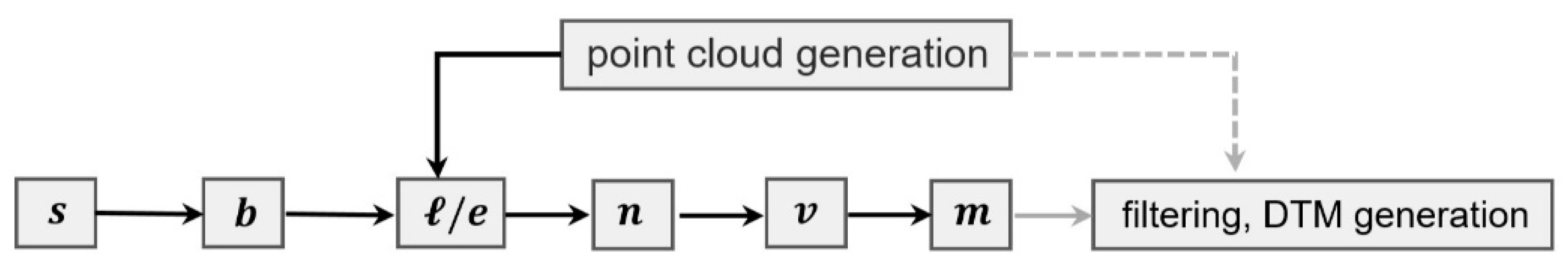
Figure 3 illustrates a sequential relation (transformations) among the “global frame” and other intermediate frames that are required for generating point cloud coordinates from the airborne laser scanning data according to users’ requirements [18,19].

As a standard data format, the point cloud data are archived and distributed in “LAS” format. Depending on the purpose in mapping, the laser spots in a point cloud are classified in order to generate the digital terrain, surface, and/or canopy models. In this process, an appropriate filtering algorithm is used [16].

In the quality of the 3D coordinates of the point cloud data, various error sources interfere. Mainly imperfections in the sensors and their assembly cause observational errors and thus decrease the accuracy of generated models [18]. Among the observed quantities, the accuracy of the laser-scanner range ($\rho$ in Figure 2b) mainly depends on the precision of time-of-flight measurements. Accordingly, the determination accuracy of the range is reported as 2 cm in average [21]. The GNSS positioning accuracy that depends on the precision of GNSS receivers as well as the GNSS processing strategies, and the precision of used IMU sensors, play a significant role in 3D coordinate accuracy of the laser scanning points. The coordinate accuracies of reference GNSS stations on the ground, which are used in relative positioning, the distance of these points to the study area, as well as the flight altitude affect the 3D position accuracy of derived point cloud. Further information on the error budget and accuracy assessment of DEM generation with airborne laser scanning technique can be found in [18] and [21]. After calculating the 3D coordinates of the laser spots as a point cloud dataset, the quality of secondary products, i.e., DSMs, DTMs, DCMs (digital canopy models), are also affected by the performance of applied filtering algorithm. Higher the reliability in outlier removal and classification in the filtering process, the higher the quality of the generated products. Süleymanoğlu and Soycan [22] provides an assessment of various filtering algorithms used for DTM generation from the airborne LiDAR point cloud, with a case study in Bergama territory. Süleymanoğlu and Soycan [22] tested six commonly used filtering algorithms and compared them in four test areas having different landscape and topographical patterns. In conclusion, the iterative polynomial fitting (IPF) algorithm was suggested for the areas having a smooth landscape, urbanized to a certain extent and agricultural patterns. However, rather than IPF, the evaluation threshold with an expand window (ETEW) filter algorithm was reported as the best performing filter method in steep areas with dense vegetation and infrastructure [22].

In literature, it is possible to find many studies on the assessment of DTM accuracy depending on various factors including GNSS data processing approach, position accuracy and the number of reference stations, filtering algorithm for blunder detection of point cloud data, interpolation and classification algorithms in DTM generating, etc. [23,24,25]. Although it changes depending on the conditions related to the aerial laser scanning experiment, the vertical accuracy by airborne laser scanning systems in open areas is reported as approximately 0.15 m root means square error (RMSE) [25,26]. However, with appropriate planning of the measurements, using precise measurement equipment and rigorous data processing strategies, the accuracies of the DTMs obtained from the LiDAR techniques can be further improved [27].

In this study, airborne LiDAR data were collected using Optech Pegasus HA-500 mounted on a Beechcraft B200 aircraft in a test flight. The measurements were organized and conducted by the general directorate of mapping [13]. Parameters of the laser sensor and flight technical data are summarized in

Table 1. Technical specifications of Optech Pegasus HA-500 laser sensor and flight data.

Laser Scanner Sensor 1
Pulse repetition rate (kHz)	100–500
Laser wavelength (nm)	1064
Scan width (FOV) (deg)	0°–75°
Scan frequency (Hz)	0–140
Sensor scan product (maximum)	800
Vertical target separation distance (m)	<0.7
Horizontal accuracy 2 (1σ)	1/5 500 x altitude
Elevation accuracy 2 (1σ) (cm)	≤5–20
Flight Data
Flight altitude (m)	1200
Groundspeed (knot)	150
Scan Pattern
Scan line spacing (m)	580
Scan width (deg)	±35°
Average density (point m−2)	≤8
Number of columns	32
Overlap	25%
Vertical accuracy (RMSE) (cm)	±7

¹ The technical specifications are obtained from Optech Pegasus HA-500 [29]. ² Dependent on selected operational parameters using nominal field of view (FOV) of up to 40°in standard conditions with 24-km visibility.

. Airborne laser scanning measurements were carried out and completed between October 23–November 6, 2014. The flight plan was prepared using flight planner software FMS planner 4.7.3 [13]. The flight altitude was planned as 1200 m, average point density was at least 8 points per m² and the flight included 32 strips with an overlap of 25%. The scan width was 35°, and the scan line spacing was 580 m.

The recorded GNSS/IMU data during the flight was processed by the general directorate of mapping using POSPac MMS (Position and Orientation System Postprocessing Package (POSPac) Mobile Mapping Suite (MMS)) software [28]. The collected GNSS/IMU data were processed and adjusted referring the two CORS-TR (continuously operating reference stations—Turkey) network stations’, AYVL (Ayvalık, latitude 39°18′41.04″N and longitude 26°41′09.96″E) and KIKA (Kırkağaç, latitude 39°06′21.24″N and longitude 27°40′19.92″E), which are in 65 km and 45 km distances, respectively, from the test site. During the postprocesses, RINEX (receiver independent exchange format) data of CORS-TR stations in 1-second sampling interval were employed [13]. General directorate of mapping preprocessed the airborne laser scanning data using LMS (LIDAR Mapping Suite) software by OPTECH, the producer company of the used laser scanning sensor. In the tests of the produced point cloud data, 51 ground points that separated as 26 control and 25 test points, were used. In the result of the preliminary tests, carried out using control points in the area, the obtained vertical accuracy by means of RMSE is reported as ±0.07 m [13]. The resulting unclassified point data were delivered by general directorate of mapping with their universal transversal mercator (UTM) projection coordinates (grid zone 35S) and ellipsoidal heights ($h$) in ITRF datum.

2.3. UAV Photogrammetry Data

In this study, a second DTM generated from the point cloud data of the General Directorate of geographic information systems was employed. As different from the first dataset, this second point cloud data were obtained with the aerial photographs from the unmanned aerial vehicle using indirect georeferencing. The horizontal coordinates of the ground control points, which were used for indirect georeferencing the point cloud, were obtained with GNSS measurements in ITRF datum. The orthometric heights of the ground control points were obtained through the leveling measurements in TUDKA99 datum. As depending on the ground control points and the indirect georeferencing of the aerial photographs, the point cloud data were generated in physical height system referring to the geoid (v-frame). Having the orthometric heights of the point cloud spots and consequently generating a second DTM in regional vertical datum was crucial for calculating the geoid heights as the difference between the two DTMs.

Aerial photogrammetry is a conventional approach widely used for 3D and 2D mapping the land parts by evaluating the photographs taken from an aerial vehicle. Similar to the aerial LiDAR technique, the photogrammetric approach is also commonly used for DTM generation in many applications. Emerging the light–weight unmanned aerial vehicles being equipped with GNSS-IMU devices and starting their use in aerial photogrammetry has significantly increased the use of this technique especially in small budget projects and applications. The fundamental theory of photogrammetric map production bases on a single image and stereo image pairs orientation. Although the fundamental outline of the theory has remained the same, the developing technologies with sensors integration opportunities led the modernization in mathematical models and calculation algorithms [30,31,32]. In the modernization manner, the “structure from motion” (SfM) algorithm resolves the 3D structure employing a series of overlapping, offset images as in the stereoscopic photogrammetry. Although this algorithm follows the same basic tenets in principle, it has fundamental differences from conventional photogrammetry by means of the solution strategy. In SfM, the camera locations, the geometry of the scene, orientation parameters are solved automatically without requiring a network of ground control points with known 3D coordinates. Instead, the listed parameters are solved simultaneously using iterative bundle adjustment having high redundancy based on a set of featured points, which are automatically extracted from the multiple overlapping images [32,33]. The development of the SfM algorithm dates back to the 1990s and bases on computer vision technology and automatic feature-matching algorithms [32]. It has been popularized through a number of cloud-processing software, which employ the SfM algorithm for generating point-cloud data for various purposes [32,34]. The advantages provided by the SfM algorithm led improvements in the quality of terrain products derived from aerial photogrammetry with UAVs [35].

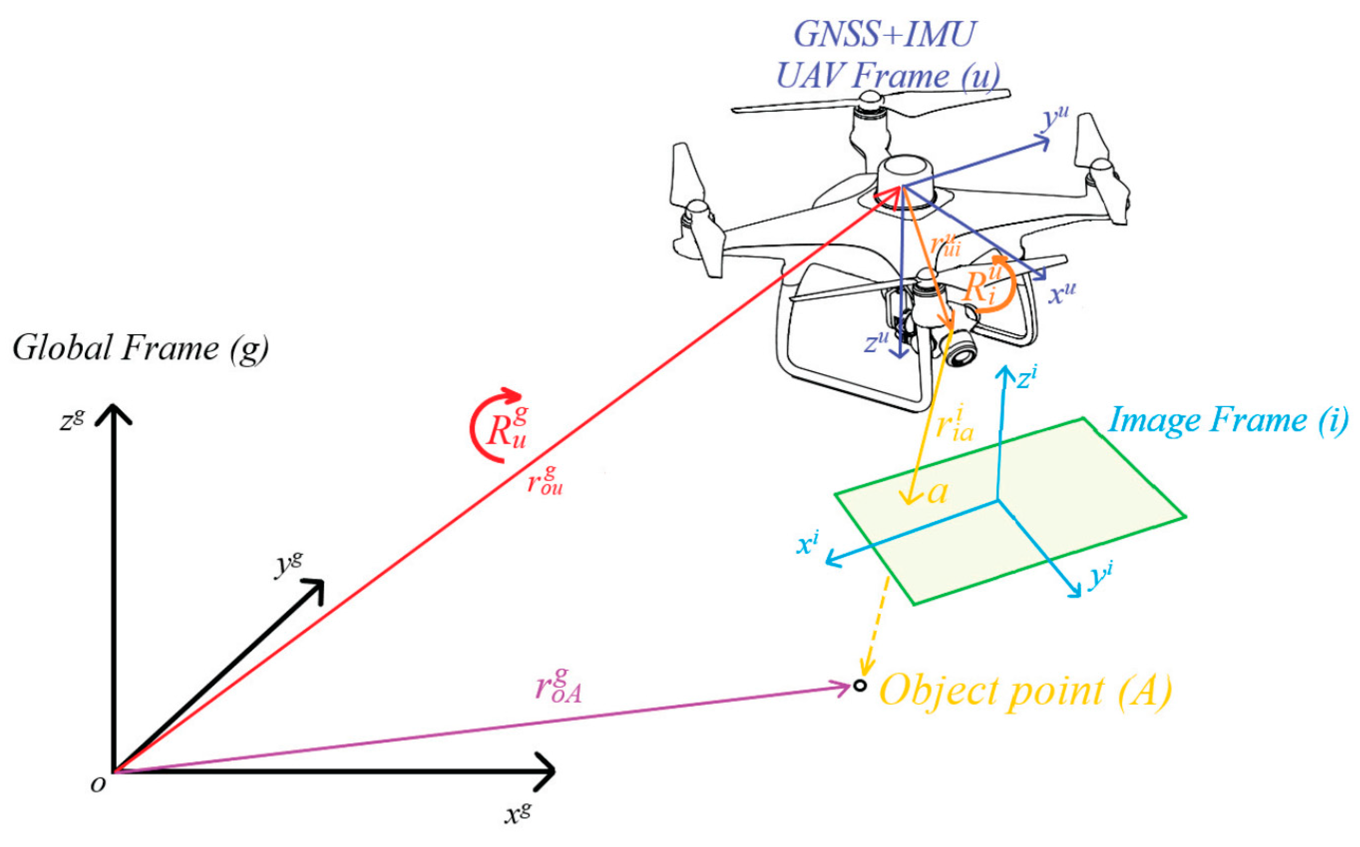
Figure 4 describes the relations between object point (A), image frame (i), UAV frame (u) and geodetic coordinate system shown as the global frame (g). Based on the described observational geometry, generating DEM grids with UAV imagery bases on a number of operational steps that involve the cooperation of different sensors including magnetic compass, barometer, CMOS camera, dual-frequency GNSS, IMU with gyroscope and accelerometer. Figure 5 shows the workflow of the process for generating the georeferenced sparse point-cloud and finally DEM through the photogrammetric method. Accordingly, after planning and carrying out the fieldwork procedures, a sparse 3D model from triangulating correspondences between multiple images in the scene is obtained with employing the SfM algorithm. Then the 3D positions of the points, which were matched with feature tracking, are recovered with the help of georeferencing. In the final section, an optimization-based procedure is applied for calculating and triangulating a dense mesh-grid data. Resulting 3D point-cloud is filtered for removing blundered points and finally, the dense point-cloud data are interpolated in order to obtain a surface model in mesh-grid form.

There are two main approaches for georeferencing the image data [36]. One of them is the indirect approach in aerial photogrammetry applications using UAVs. In this method, the image data are georeferenced indirectly using ground control points (GCP) having known coordinates that are visible on images. For indirect georeferencing, the aerial vehicle is not necessarily to be equipped with position and orientation instruments and this is assumed as an advantage. Accordingly, indirect georeferencing provides accurate positioning results in required geodetic datum depending on the accuracy and reference datum of the used ground control points’ coordinates. The indirect georeferencing process is formulated in Equation (2).

$$r_{oA}^g=r_{oi}^g\left(t\right)+s_{A }{R}_i^g\left(t\right)r_{ia}^i\left(t\right)$$

(2)

where $r_{oA}^g$ represents the ground coordinates vector of the object point (A) in geodetic coordinate system (g-frame), $r_{oi}^g\left(t\right)$ is coordinates vector of camera sensors at the time ($t$) in $g$-frame, $R_i^g\left(t\right)$ is the rotation matrix of i-frame to g-frame, $s_A$ is scale factor, $r_{ia}^i\left(t\right)$ represents the object coordinates vector in $i$-frame (see Figure 4).

On the other hand, the second approach is the direct georeferencing. This approach uses onboard sensors for image georeferencing. In this approach, the exterior orientation is typically measured using a GNSS set and an INS unit mounted on the aircraft body. This method requires accurate sensors time synchronization and misalignment calibration.

Direct georeferencing for obtaining ground coordinates of the object point (A) in the geodetic coordinate system (g-frame), relies on the Equation (3). Using this equation in the direct approach requires a priori knowledge of a number of systematic parameters ($s_{A }$, $r_{ui }^u$) stated in the equation [37].

$$r_{oA}^g=r_{ou}^g\left(t\right)+R_u^g\left(t\right)\left(s_{A }{R}_i^u\left(t\right)r_{ia}^i\left(t\right)+r_{ui }^u\right),$$

(3)

where $r_{ou}^g\left(t\right)$ is coordinates vector of GNSS-IMU sensors at the time ($t$) of exposure, $R_u^g\left(t\right)$ is the rotation matrix of u-frame to g-frame, $R_i^u\left(t\right)$ is the rotation matrix from of i-frame to u-frame, $r_{ia}^i\left(t\right)$ is the object coordinates vector in $i$-frame, $r_{ui }^u$ is the position vector of camera projection center in u-frame (see Figure 4). The $r_{ui }^u$ lever-arm and $R_i^u$ boresight parameters in $u$-frame are constant.

In each step of the 3D point cloud generation process in UAV photogrammetry, different factors including input data, image quality, GNSS position accuracy, employed processing parameters affect the final DEM accuracy. Considering the experimental results on accuracy assessments of DEMs generated by UAV photogrammetry imagery, it is seen that ~5–6 cm vertical accuracy in RMSE can be obtained in bare areas with moderate topography [39].

Following the described methodology and indirect georeferencing procedure, 3D coordinates of the point cloud were derived using UAV photogrammetry by the General Directorate of geographic information systems of Turkey. The vertical accuracy of the point cloud data were reported as ~5–6 cm by the data provider institution. The dataset was provided with their universal transversal mercator (UTM) projection coordinates (grid zone 35S) in ITRF datum and orthometric heights ($H$) in Turkey national vertical control network (TUDKA99) datum. The density of the provided point cloud was 450 points per m².

2.4. DTM Generation from Point Cloud Data for Modeling Local Geoid Surface

In the tests, the local geoid surface was derived from the differences between two DTMs, that were generated with point cloud data by aerial laser scanning $(DT{M}_I)$ (Section 2.2) and UAV photogrammetric imagery ($DT{M}_{II}$) (Section 2.3), respectively. The point heights, obtained from $DT{M}_I$ are the geometrically meaningful ellipsoidal heights ($h$) in ITRF datum and refer to GRS80 reference ellipsoid, whereas the $DT{M}_{II}$ provided us the physically meaningful orthometric heights ($H$) in regional height datum TUDKA99. Hence the local geoid heights ($N$) were generated from the differences of $h$ and $H$ as $N=h-H$ in meter (see Figure 6 for the definition of geoid height $N$ at a topography point).

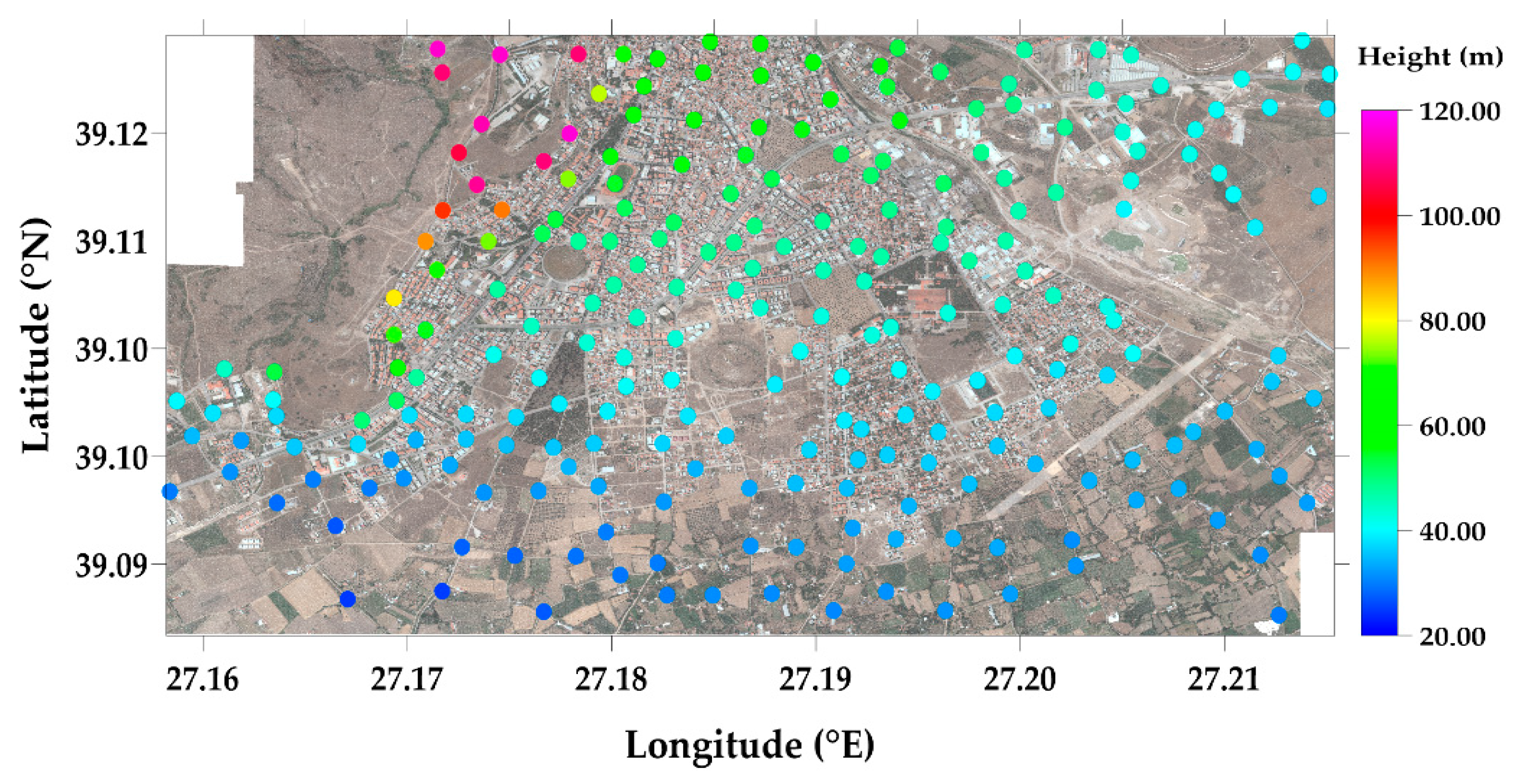
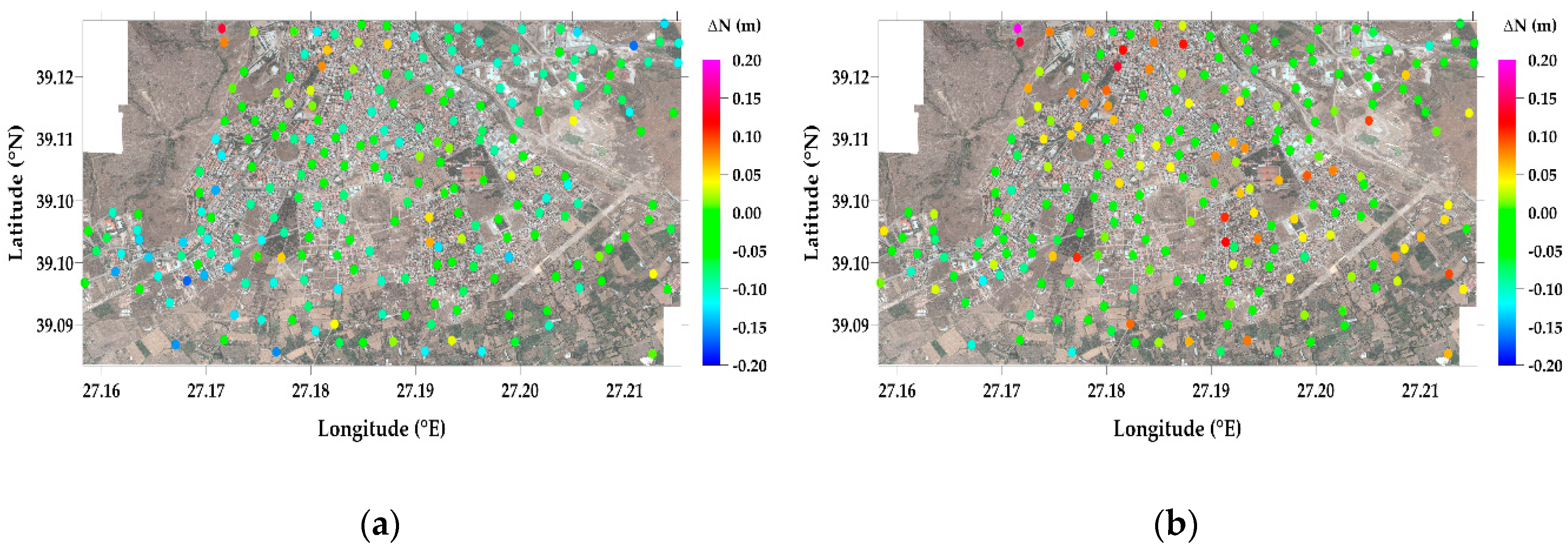
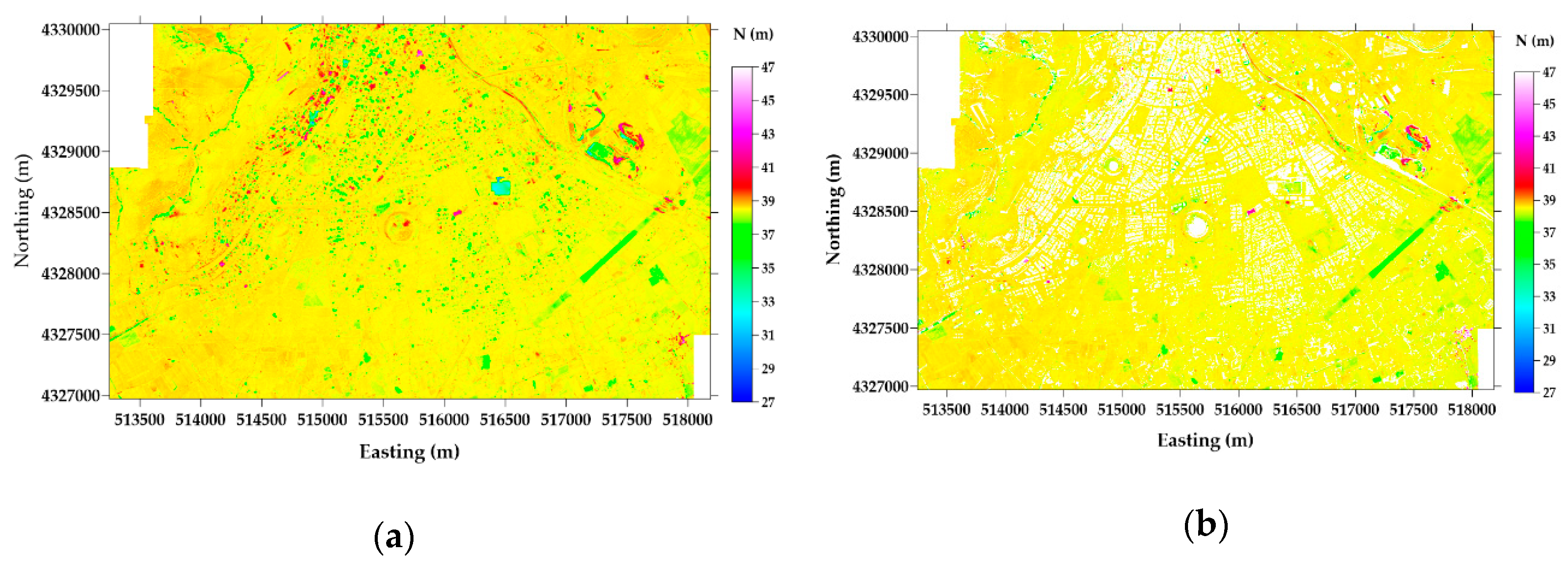
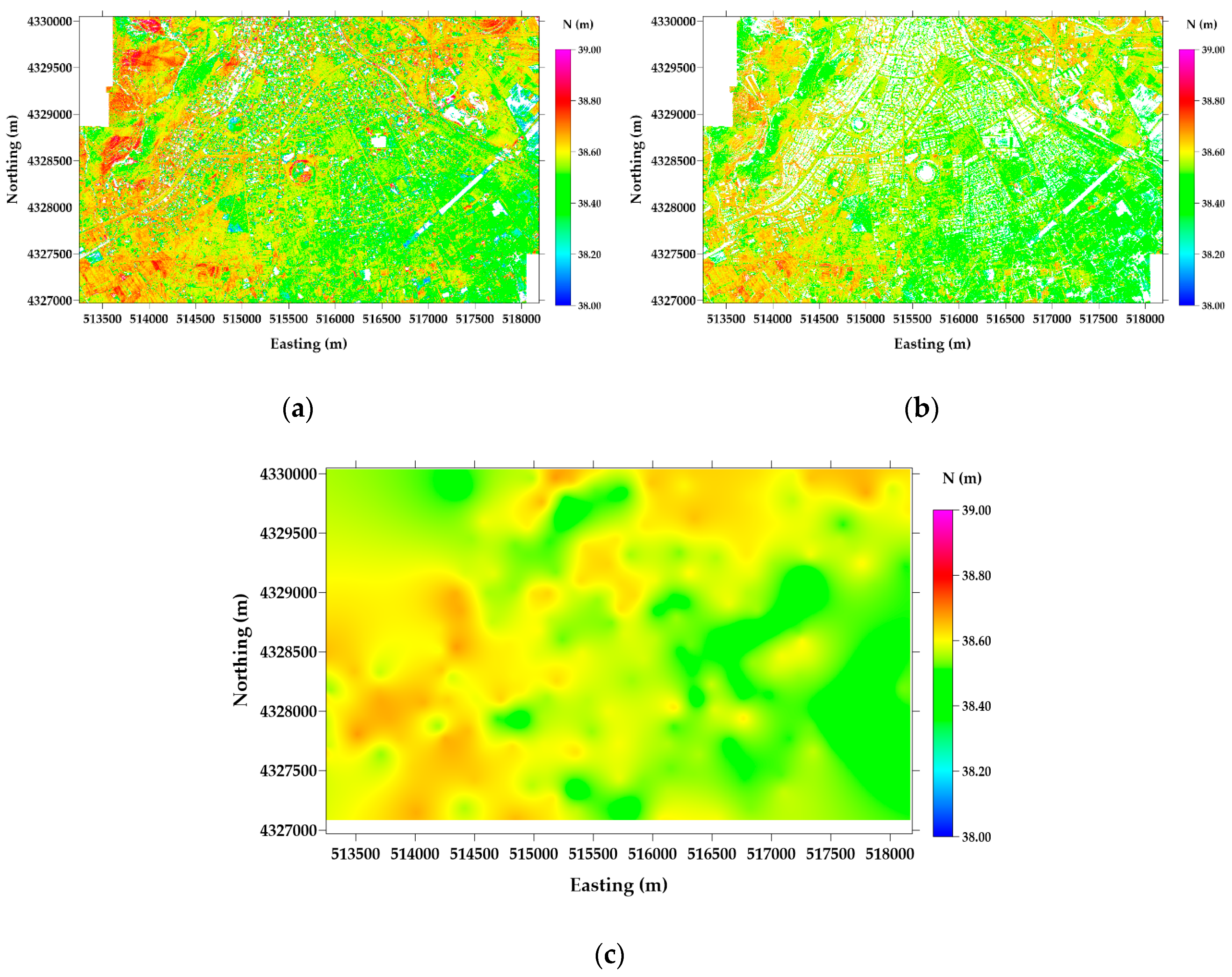
With following the described procedure, based on differences of $DT{M}_I$ and $DT{M}_{II}$, the local geoid models in grids and pointwise formats were generated. Numeric tests carried out using the grid models aimed to evaluate the performance of the produced models along the entire area which involves various land cover types. On the other hand, the pointwise local geoid models were calculated at the manually selected points at the bare topography. Thus, the numeric tests with the local geoid models in pointwise format were expected to provide more realistic and reliable results regarding the performance of the suggested geoid modeling methodology. The distribution of the manually selected 250-geoid control points in the study area is shown in Figure 7. As will be explained in detail below, the numeric tests carried out with the local geoid models in gridwise format also show the assessment results of the two different classification methodologies used in DTM generation. Accordingly, the two DTM couples generated using both progressive densification and morphologic filter algorithms, respectively, were used in deriving the two gridwise local geoid models. The obtained geoidal heights from each DTM couple were investigated through their basic statistics in the following. Both filter algorithms, as their theories are mentioned in the following, were implemented with separate software.

After obtaining the point cloud data from the data provider institutions, in the first step of the processes, the data were filtered and the DTMs were generated accordingly. The original point cloud by aerial LiDAR measurements was given to us in divided tiles. However, the second point cloud obtained from UAV photogrammetric imagery covered the entire area and provided as a single dataset for the whole area. Since the study area is rather large and therefore processing dense point clouds as a whole requires high-capacity computer processors and lengthy processing time, we divided the UAV point cloud data into 1 km × 1 km subareas at first for the filtering process. Thereafter, the piecewise DTMs generated as separate tiles were connected in order to constitute the DTM of the whole area. The gaps, which were at the tile boundaries, were interpolated from the DTM data in neighboring map sheets. However, since it was recognized that the interpolation process was unsuccessful for providing smooth and seamless transition along the tile boundaries of the DTMs, the computation strategy was altered and the DTMs were generated using the point cloud data as a whole, after blunder removal and denoising the partitioned point cloud data. As mentioned above, the generation of DTMs was carried out using two different filtering approaches in classification. In different stages of the point cloud data processing and then the DTM generating: CloudCompare, Envi LiDAR, Global Mapper GIS software were used [40,41,42]. In calculating local geoid models both in gridwise and pointwise formats by subtracting the orthometric heights of the $DT{M}_{II}$ from the ellipsoidal heights of the $DT{M}_I$, the Surfer software by Golden Software company was employed [43]. We selected 250 geoid control points on bare topography with homogeneous distribution over the area for generating the pointwise version of the local geoid model. While determining the locations of these scattered points set, we paid special attention to include the characteristic points of the topography that can be assumed to be remained unchanged, and thus to be measured during both the aerial LiDAR and UAV photogrammetry campaigns (Figure 7). In this way, we aimed to use the topographic points, which are common in both datasets and hence to eliminate the effect of possible environmental changes within a short time-lag between the airborne and UAV flights in the results.

In the filtering step of the point-clouds, the noise and blunders in the point clouds were cleaned using statistical outlier removal (SOR) filter algorithm in CloudCompare software [44]. SOR filter has a rather simple computation algorithm that bases on stochastic analysis of all points in the point cloud and removes the points, which do not satisfy the assigned threshold as the criterion, from the point cloud [45]. In filtering, for each point in the point cloud, the spatial distance to a number of neighboring points are calculated. The average of the calculated distances is taken into account. The distribution of the differences between the calculated distances from their average is assumed as Gaussian. Then any point having a distance difference, which does not fit the distribution is removed as a blunder. Therefore, the distance between a points-couple constituted based on the assigned number of points for defining the neighborhood boundaries (let us say $k$ points around the point in question) cannot exceed $d_{max.}$ in meter that:

$$d_{max.}=\mu +n\times \sigma$$

(4)

where $\mu$ is average distance, $n$ = 1,2,3 is a multiplier constant that is selected depending on the required interval of confidence, $\sigma$ is the standard deviation of the distances. Hence, the points which are farther than $d_{max.}$ are removed. In the process, the definition of $k$, the number of points in the neighborhood and $n$, the multiplier of standard deviation, are critical parameters that determine the number of points, deleted from the dataset. Hence, the success of the filtering process. In the study, in a result of a trial-and-error-based approach, we determined and used as $k$ = 6 and $n$ = 1, with concerning to reach the required accuracy from the generated DTMs according to our purpose. After removing the blunders with applying distance-based statistical outlier removal filter, we ran a SOR-like filter algorithm for further denoising of the point cloud data in order to obtain higher accuracy DTM data in result [46]. The formulation of the denoising algorithm, which was applied after distance-based outlier detection filter, is similar to the SOR filter. As different from the first step, the denoising filter takes the height differences among the points into account instead of the distances and remove the points having the height difference exceeding the threshold value ($h_{max.}=\mu +n.\sigma$, where $\mu$ is the average value of height differences, $n$ is multiplier constant, $\sigma$ is the standard deviation of height difference from their average value). In applying the denoising filter, the number of points in the neighborhood was chosen 6 and the multiplier constant was 1 too.

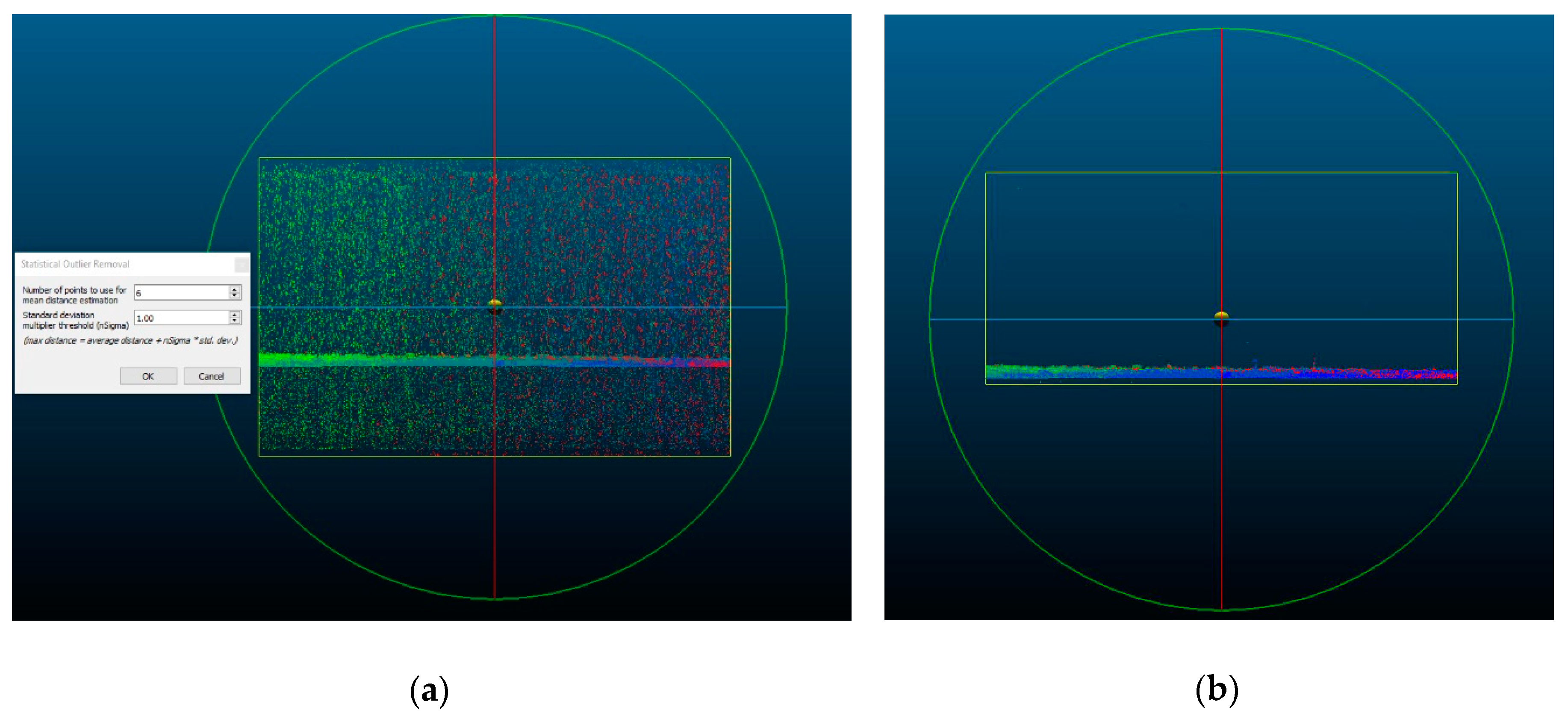
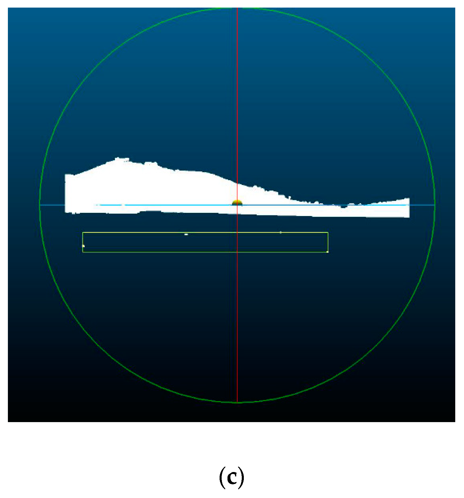
After removing the blunders and denoising the data, the number of points in the point cloud decreased. As an example, in the point cloud derived from UAV photogrammetric imagery, while the number of points was 23,175,329 in the original dataset, it reduced to 18,231,092 after filtering. Thus, 21% of all points were removed with filtering. After the stochastic-based filtering, which was carried out automatically using SOR and denoising filters in CloudCompare software modules, the remained points in both point cloud datasets were also visually detected once again and a few more points, which were suspected to be outliers, were removed manually using the same software. The point cloud in view of the vertical section before (a) and after (b) the automatic and manual (c) cleaning processes are shown in Figure 8 [46]. This visualization gives an idea of the success of the applied filters and the need for manual intervention after automatic cleaning of the data.

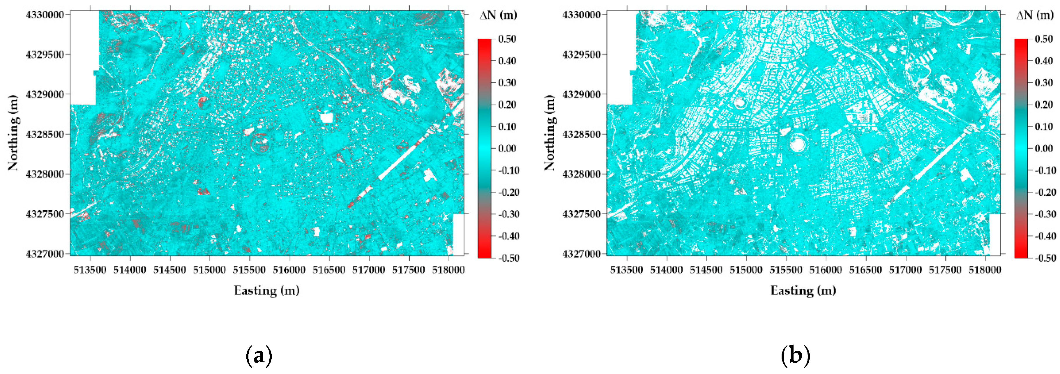
Following the filtering and denoising processes of the point clouds, the DTMs from aerial LiDAR and UAV photogrammetry point clouds were generated separately in raster (*.geotiff) format. In this stage, the DTM generation process was carried out through different filter algorithms and obtained results were assessed in order to clarify the difference between the applied algorithms by means of calculated geoid heights [40,47]. As was mentioned above, in the piecewise generation of the DTMs, the artifacts occurred along the tile boundaries on the DTM pattern (see Figure 9). Because of these artifacts, in a second trial, the piecewise point cloud datasets were combined after filtering and denoising processes and then the DTMs were generated using point clouds as a whole in the study area. In order to optimize the computational time and computer processor usage, the point densities of the point clouds were partly decreased [46].

In the classification for DTM generation, first, the progressive densification filter with adaptive triangulated irregular network (ATIN) algorithm was applied using Envi LiDAR software [22]. Following the generation of DTMs from both aerial LiDAR and UAV photogrammetry point clouds using Envi LiDAR software, the same production was repeated with morphologic filter by using Global Mapper software [22,40].

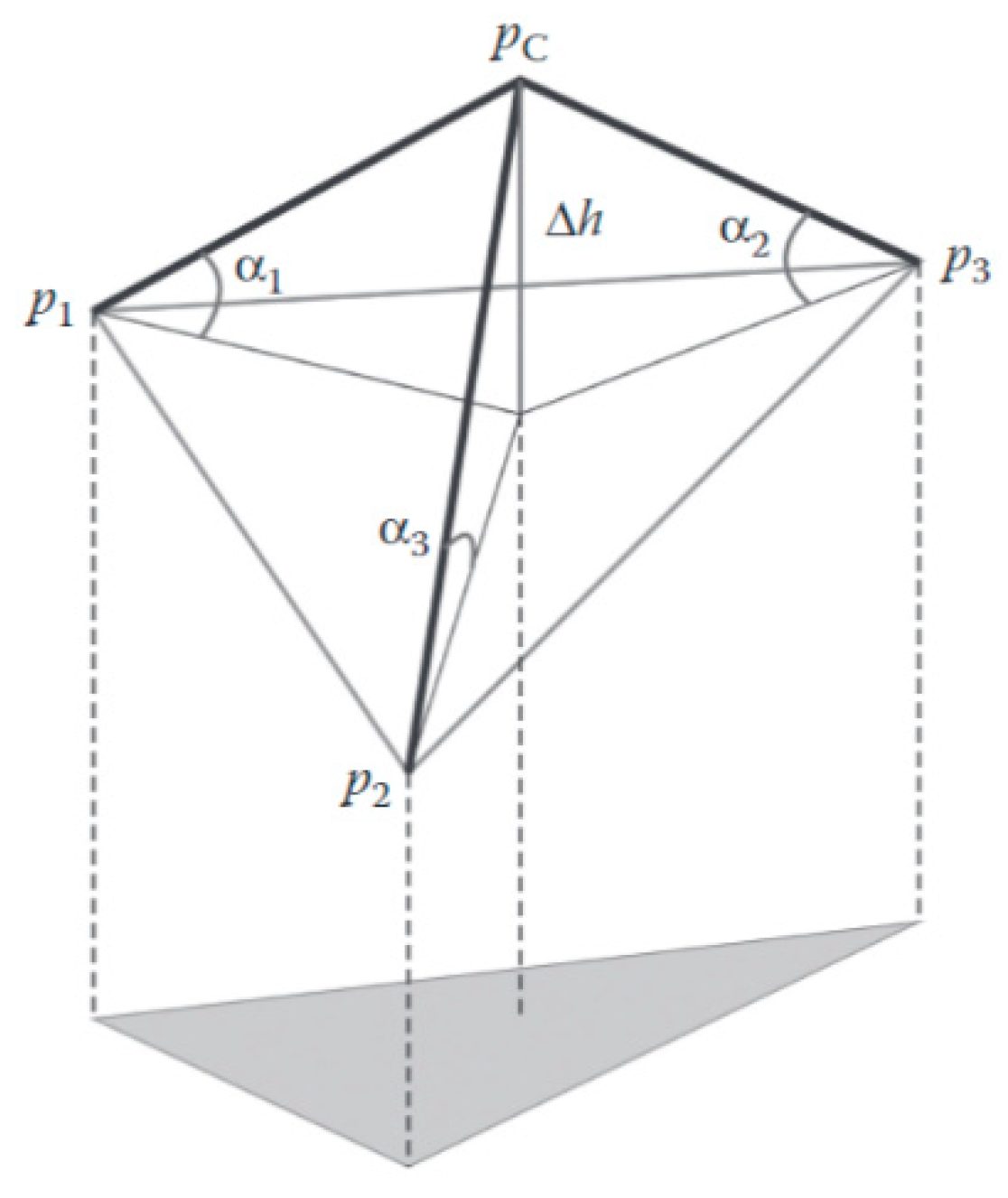
Basically, in the progressive densification filter with the ATIN algorithm, the study area is divided into subareas and the minimum elevation is locally determined. The points with minimum elevation are assumed to be ground surface points (bare topography surface). Then triangulated irregular network (TIN) is generated using the Delaunay triangulation method. Considering the distance of a point (but except the seed point) in a Delaunay cell to the TIN surface ($\mathsf{\Delta }h$) and the widest of the three angles (${\alpha }_i$) with the TIN surface (see Figure 10), it is decided whether to keep or remove the point ($p_c$). In order to make this decision, the distance and angle at the point in question are compared with predefined threshold values. If the compared values are smaller than the threshold values, the point is assumed as the ground point. This filtering algorithm is an iterative process and each time when a point is removed from the ground points dataset, the TIN is regenerated, and the process continues until all points are classified as ground or object detail [48].

Beside of the progressive densification, the morphologic filter that we applied in DTM generation with Global Mapper software, is also mentioned in four filtering algorithm categories given in [48]. Morphologic filtering algorithm bases on mathematical morphology principles and mainly uses two operations, erosion (⊖) and dilation (⊕). According to the sequential use of these operators, closing (erosion-dilation) and opening (dilation-erosion) operations are applied. In the progressive morphologic filtering algorithm, the points having minimum height values in a window are chosen and an approximate surface as geometric locations of these points is determined. Secondary surfaces are generated by carrying out an opening operation to the initially described surface. The two surfaces are compared considering a threshold value ($\mathsf{\Delta }{h}_{max.}$) and the points below the threshold value are categorized as ground points. Not only the height difference threshold value, but also the window size selection is also critical to achieving good results in a morphologic filter. The size of the selected window can be enlarged according to the size of the largest object in the workspace in order to detect and filter the non-ground objects effectively [49]. In practice, along the filtering process, the window size is increased gradually. Because the morphologic filter with fixed window size is capable to detect and remove the measurements for the buildings and trees from the point cloud data, however, it is difficult to detect all non-ground objects having various sizes. Increasing the window size is a solution for increasing the effectiveness of the filter. The ground points are differentiated by comparing the points’ value with the threshold. The height difference threshold can be determined considering the slope of topography in a study area. Assuming the slope as constant, the relation between the maximum height difference ($d{h}_{max\left(t\right),k}$) for the terrain ($t$), window size ($w_k$) at $k^{th}$ iteration and terrain slope ($s$) is formulated as:

$$s=\frac{d{h}_{max\left(t\right),k}}{\frac{\left(w_k-w_{k-1}\right)}{2}}$$

(5)

and accordingly, the height difference threshold $d{h}_{T,k}$ is:

$$d{h}_{T,k}=\{\begin{array}{c}d{h}_0, \\ s\left(w_k-w_{k-1}\right)c+d{h}_0,\\ d{h}_{max},\end{array} \begin{array}{c}if w_k\le 3 \\ if w_k>3 \\ if d{h}_{T,k}>d{h}_{max}\end{array}$$

(6)

where $d{h}_0$ is the initial height difference threshold, $s$ is the slope, $c$ is the cell size and $d{h}_{max}$ is the maximum height difference threshold [49].

Applying the addressed classification filters, the DEMs ($DT{M}_I$ and $DT{M}_{II}$) with 1-m grid resolution covering the entire study area were generated from aerial LiDAR and UAV photogrammetry point cloud data, respectively, using Envi LiDAR (the progressive densification filter with ATIN algorithm) and Global Mapper software (progressive morphologic filtering algorithm). In the results, Global Mapper software was found more successful in extracting and removing the artificial objects in order to obtain the DTMs. The superior accuracy of DTMs, generated with the Global Mapper Software and the morphologic filter is clear in the statistics from the local geoid model test results (please see in Section 3).

2.5. Regional Geoid Models Used in Validations

Geoid models can be determined using one of a few methods given in the literature and available to the users either as an analytical function or as a raster form [10]. In geodetic applications the geoid height parameters ($N$) obtained from a suitable geoid model are used for various purposes including the transformation of GNSS ellipsoidal heights to the physical heights that are in the regional vertical datum, calculating corrections and reductions of the terrestrial observations to a reference surface, inspecting the Earth’s interior, observing and predicting Earth-mass transfer, etc. As depending on the required accuracy of height information, an appropriate geoid model is chosen and used in computations. In many engineering projects, geodetic infrastructure establishment studies and large scale mapping applications, the required geoid model accuracy is lower than 5 cm, whereas in studies such as in geographic information system establishment, archeological surveys, forest applications, a geoid model with decimeter or sub-decimeter level accuracy may satisfy the required vertical accuracy [50]. 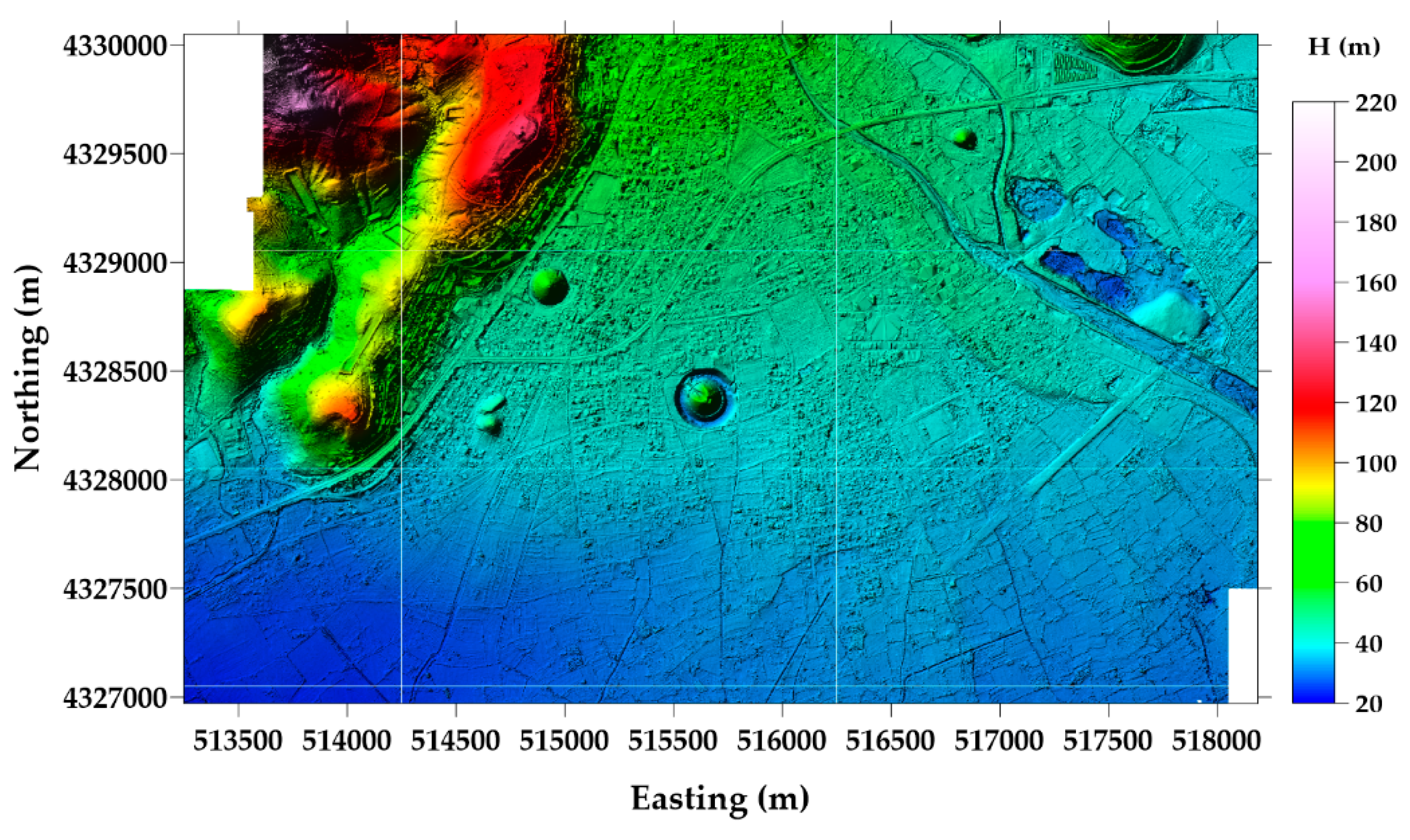Parallel to the advances in GNSS techniques and their use in mapping and surveying applications, many countries serve the high-accuracy regional geoid model to the practitioners and surveyors as part of their national geodetic infrastructure in order to support and increase the efficiency of satellite-based positioning techniques in geodetic and surveying applications [51,52]. In Turkey where the study area is located in the west of the country (Figure 1), the accuracy of the most recent publicly available regional geoid model (Turkey Geoid 2003– TG03) is ~ 8.0 cm. This accuracy is not sufficient for the large scale maps and spatial data production studies and most of the engineering projects [14].

TG03 is one of the geoid models that was used in this study. It was compared with the derived geoid models from generated DTMs in gridwise and pointwise formats, respectively. The TG03 model was calculated by the general directorate of mapping and released to the civilian users as the most recent official regional geoid model of Turkey in 3 arc-minute resolution grid data. This model was calculated using the remove-compute-restore (RCR) method with the least-squares-collocation (LSC). The used data included the terrestrial gravity observations distributed over the country having ~7–8 mGal accuracy and ~30 arc-second spatial resolution in modified Potsdam gravity datum [53,54]. In addition, the marine gravity data derived from satellite altimetry products by ERS1, ERS2, and TOPEX/POSEIDON satellite observations at the surrounding seas were employed to complete the land gravity dataset in computations. EGM96 with harmonic expansion degree ${\ell }_{max.}$= 360° was used as a reference geopotential model for TG03 [55]. In order to consider the high-frequency contribution of the topographic masses in the model, the DTM data having 450-m spatial resolution grids on land and dense bathymetry data in shoreline areas were employed [53]. Involving a number of GNSS/leveling data sparsely distributed over the country in computations, the geoid heights by TG03 model fitted to the ITRF96 coordinate datum and the regional vertical datum of Turkey (TUDKA99). 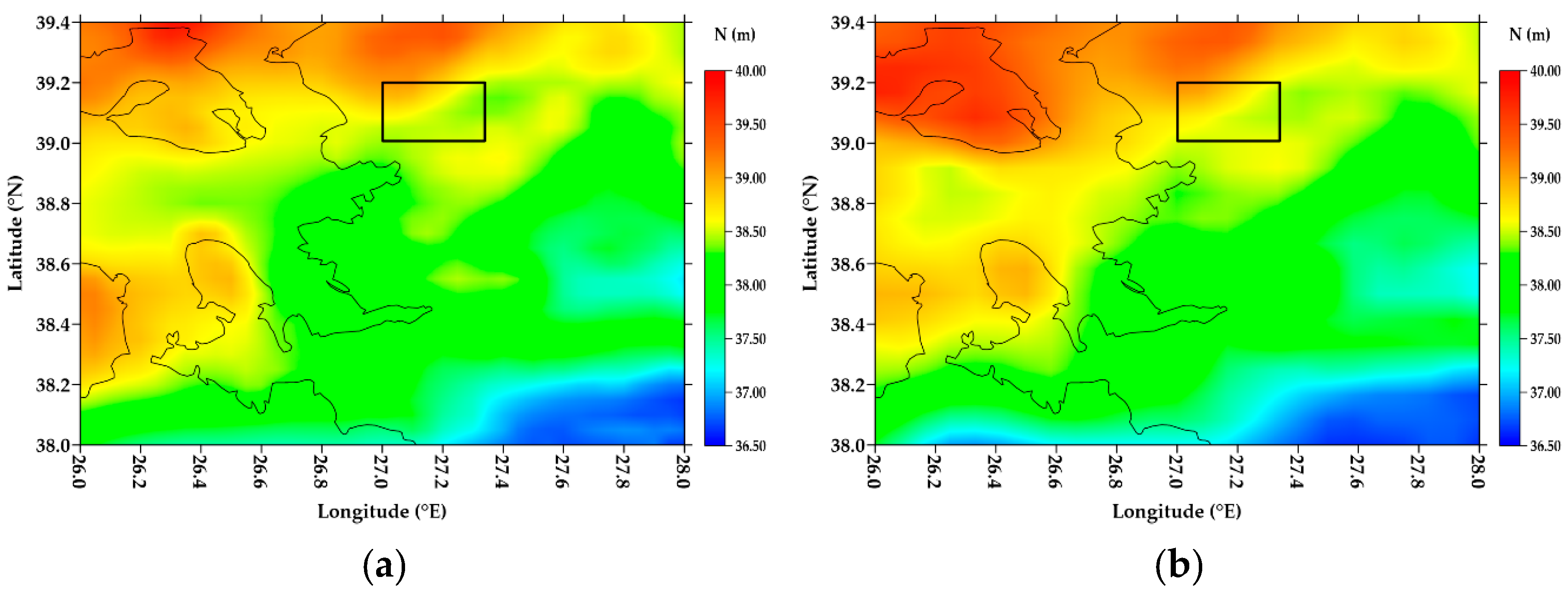The geoid height values at the scattered geoid control points (see in Figure 7) were interpolated from the TG03 grid nodes using the inverse distance weighting method and compared with calculated geoid heights derived from the local geoid models by DTMs differences [56]. Since the TG03 model has already been served as grid-data, the comparison results of the local geoid models in grid form with the TG03 model were easily generated at grid nodes and visualized as “geoid height difference surfaces” in Section 3.

In certain applications where decimeter level geoid model accuracy is sufficient, global geopotential models ($N\approx N_{GGM}$) may provide the required accuracy. Global geopotential models are released as spherical harmonic expansion equations with coefficients up to certain degree/order (d/o). The accuracies of these global models were significantly improved since 2000 with data contribution of Earth gravity field satellite missions, namely CHAMP, GRACE, GOCE and recently GRACE-FO [57]. Equation (7) provides the mathematical formulation of the geoid height value by means of spherical harmonic expansion coefficients [9].

$$N_{GGM}=\frac{GM}{r\gamma }{\displaystyle \sum }_{\ell =2}^{{\ell }_{max}}{\left(\frac{a}{r}\right)}^{\ell }{\displaystyle \sum }_{m=0}^{\ell }\left(\mathsf{\Delta }{\overline{C}}_{\ell m}cosm\mathsf{\lambda }+{\overline{S}}_{\ell m}sinm\mathsf{\lambda }\right){\overline{P}}_{\ell m}\left(cos\theta \right)$$

(7)

where (θ, λ, r) are co-latitude, longitude and geocentric radius of the computation point, respectively; $a$ is the major axis radius of the reference ellipsoid; GM is the product of the gravitational constant and the mass of the Earth; $\mathsf{\Delta }{\overline{C}}_{\ell m}$ and ${\overline{S}}_{\ell m}$ are the fully normalized spherical harmonic coefficients, related to the normal potential of the reference ellipsoid from a specific degree of $\ell$ and order m, ${\overline{P}}_{\ell m}\left( cos\theta \right)$ are the fully normalized associated Legendre functions. The global geopotential models with their spherical harmonic coefficients are obtained from a number of international data centers. The International Center for Global Earth Models (ICGEM) serves an almost complete list of the geopotential models, which were released since 1966 [15].

In numeric tests of this study, one of the high-resolution geopotential models, EIGEN6C4 (${\ell }_{max.}$=2194) (EIGEN=”European improved gravity model of the earth by new techniques”), was evaluated and compared with the local geoid model derived from the photogrammetric techniques [58]. The spatial resolution of the model corresponding to its maximum expansion degree is ~9 km. In the maximum expansion degree, its reported accuracy by means of RMSE of geoid height differences in Turkey is ~12 cm [57]. In the numeric tests of the study, EIGEN6C4 (with d/o of 2194) was employed and the geoid heights (Equation (7)) from the model were calculated both at the geoid control points (Figure 7) as well as at the grid nodes for surface-based comparisons. In calculation with the geopotential model, ICGEM calculation service was used [15]. The calculated geoid heights referenced to the ITRF datum (GRS80 reference ellipsoid), in order that they were comparable with the local geoid models by the photogrammetric techniques.

After calculating the geoid models, another critical process is validating their accuracy using independent data and appropriate method before releasing these models to the users. Independent high-accuracy ground datasets are required to evaluate their external accuracy. In this purpose high-accuracy GNSS/leveling data, astrogeodetic deflections of vertical values, as well as sea-level observations at tide-gauge stations (for validations along the coastline) are commonly used [12]. However, local geoid data derived from the photogrammetric techniques have not been employed for either determination or validation of the geoid models so far. In this manner, the numeric tests, which were carried out for clarifying the usability of the DTMs derived from the photogrammetric techniques in geoid modeling and validations make an original contribution to the geoid determination studies. The following chapter discusses the obtained results from the numeric tests of local geoids by aerial LiDAR and UAV photogrammetry DTMs.

3. Results and Discussion

3.1. Local Geoid Model Accuracy Evaluation According to DEM Generation Strategy

In the first part of the numeric tests, the DTMs from point clouds were generated for local geoid model determination. In their generation, two different filtering algorithms were used in the classification. One of the algorithms was the progressive densification filter with the ATIN algorithm, applied using Envi LiDAR software [47]. The other was the progressive morphologic filtering algorithm applied using Global Mapper GIS software [40]. In results, the two DTMs by aerial LiDAR data were in hand for obtaining the ellipsoidal heights of the terrain points. On the other hand, the two DTMs by UAV photogrammetric imagery were for providing the orthometric heights of the same points in TUDKA99 datum. Accordingly, two local geoid surface models were generated using the DTM-couples ($N=h_{{\mathrm{DTM}}_{\mathrm{I}}}-H_{DT{M}_{\mathrm{II}}}$) by Envi LiDAR and Global Mapper outputs, respectively.

Figure 11 shows the calculated local geoid surfaces using DTMs generated by Envi LiDAR (a) and Global Mapper (b), respectively.

Table 2. Statistics of calculated geoid heights from models using Envi LiDAR and Global Mapper software over the whole test site (m).

Geoid Model by	Minimum	Maximum	Mean	Std. Deviation
Envi LiDAR	26.099	48.610	38.506	0.481
Global Mapper	−5.925	50.567	38.507	0.291

gives the statistics of the calculated local geoid heights at grid nodes (1-m spatial resolution) along with the whole test site. However, considering the geoid model surfaces in Figure 11 and their maximum, minimum values in Table 2, it was concluded that the geoid models, derived from two different software, included blunders. Thus, blunder detection with one sigma (1-$\sigma$) test was applied and the geoid height values, which deviate from the mean geoid height value in the area more than 1-$\sigma$ (corresponds to keep the points having geoid height values within 68% confidence interval), were removed from each dataset. The geoid height surfaces after the 1-$\sigma$ test and their statistics are given in Figure 12 and

Table 3. After removing blunders with 1-$\sigma$ test: the statistics of calculated geoid heights from models using Envi LiDAR and Global Mapper software over the whole test site and point-wise geoid heights interpolated from Global Mapper grid-wise solution (m).

Geoid Model by	Minimum	Maximum	Mean	Std. Deviation
Envi LiDAR	38.029	38.979	38.552	0.143
Global Mapper	38.215	38.798	38.533	0.102
point-wise	38.424	38.691	38.572	0.055

, respectively.

When the obtained statistics in Table 2 and Table 3 are compared, it is seen that removing the blunders using 1-$\sigma$ test succeeded and the two local geoid model surfaces by Envi LiDAR and Global Mapper are closer to each other now. However, comparing the statistics of two geoid model surfaces in Table 3, the distribution of geoid heights by means of their standard deviations differs with ~4.1 cm that is actually significant for local geoid modeling purposes in geodetic applications.

In the last row of Table 3, the statistics of geoid heights derived at scattered geoid control points that their distribution is seen in Figure 7, are given. The geoid heights at these geoid control points were calculated with interpolation from the local geoid surface model by the Global Mapper grid-wise solution.

In Figure 12c, the pointwise local geoid surface is shown. This surface was generated by interpolating the geoid height values at the scattered geoid control points given in Figure 7. In calculating the surface model, the geostatistical Kriging algorithm in Surfer software was applied. From this figure, the change amount and slope direction of the local geoid surface are recognized. This pattern of the local geoid surface derived from photogrammetric approaches was compared with the regional geoid model (TG03) (the TG03 geoid model surface is shown in Figure 13a) and the global geoid model (EIGEN6C4) (global geoid model surface in Figure 13b). Compared Figure 12 and Figure 13, it is seen that all three geoid surface models have the same characteristic trend, but in varying levels of details. Because the local geoid surface is more detailed (Figure 12c) and the compared to local geoid, the regional geoid surface is smoother (Figure 13a) and the global geoid model surface is naturally the least detailed surface model (Figure 13b) in the considered area. Since this figure was generated as depending on rather dense data points, the smooth character of the local geoid surface can hardly be recognized in Figure 12c. When Figure 7, Figure 12c and Figure 13a,b are considered together, it is confirmed that the descending trend of the geoid surface from north to south follows the topographic heights shown in Figure 7 with changing colors of the point symbols.

3.2. Comparisons of Local Geoid Models by the Photogrammetric Techniques with Regional and Global Geoids

In the second part of the numeric tests, the local geoid models generated using the photogrammetric techniques were compared with regional geoid model, TG03 and a global geopotential model, EIGEN6C4 (${\ell }_{max.}$= 2194), and statistics obtained from these comparisons clarify the fitting performance of the compared models each other. Erol et al. [54] tests the TG03 model using high-accuracy GNSS/leveling data in a larger area very close to our test site and reports external accuracy of TG03 ~8.0 cm in terms of RMSE of geoid height differences at GNSS/leveling benchmarks. Erol et al. [57] validates a high resolution geopotential model, EGM2008 (${\ell }_{max.}$ = 2194) [59], using the same GNSS/leveling dataset in the area close to the Bergama test site and reports its external accuracy as ~12.0 cm by means of RMSE. Although the external accuracy of the EIGEN6C4 has not been published in this article [57], in its preparation, this geopotential model having equal expansion degree/order with EGM2008 has been validated as well. In the unpublished results, it has been seen that EIGEN6C4 revealed almost the same accuracy with EGM2008. The reasons for these two global models having similar accuracies is that the spherical harmonic expansion degrees of both geopotential models are the same and almost similar datasets were used in their calculations. As a conclusion of this, we assumed the external accuracy of EIGEN6C4 model as ~12.0 cm in the test site in this study as well.

The accuracy of the ellipsoidal heights obtained from the aerial LiDAR point cloud is reported as 7.0 cm in [13]. Regarding the personal communication with the data provider of the UAV photogrammetric imagery point cloud, the accuracy of the orthometric heights obtained from the UAV photogrammetry point cloud is ~5–6 cm. According to known accuracies of the data, we estimated the accuracy of geoid heights generated using local geoid models with error propagation principles: ${\sigma }_N=\sqrt{{\sigma }_h^2+{\sigma }_H^2}$ = ~9.2 cm. In this case, the local geoid models calculated in this study are assumed comparable with TG03 and EIGEN6C4 models by means of accuracy and have the capability for validating these regional and global models.

Figure 14 shows the difference between the generated local geoids from two software and regional geoid (TG03) model surfaces. In Figure 14a TG03 model surface is compared with the Envi LiDAR local geoid surface and in (b) it is compared with the Global Mapper local geoid surface. Comparing the geoid height differences maps and considering the distribution of the differences over the area, we can say that the local geoid surface calculated with Global Mapper software fits the TG03 model surface better. This result is confirmed by the fitting statistics given in

Table 4. Statistics of geoid height differences between local geoid models (Envi LiDAR and Global Mapper, respectively) and regional Turkey Geoid (TG03) (m).

Geoid Height Differences	Minimum	Maximum	Mean	Std. Dev.
Envi LiDAR − TG03	−0.516	0.573	−0.029	0.139
Global Mapper (GM) − TG03	−0.330	0.386	−0.010	0.098
point-wise (GM) − TG03	−0.156	0.049	−0.059	0.046

. The mean values of differences show that the local geoid surfaces do not include a systematic shift from TG03 and their datums are quite compatible. The last row of Table 4 shows the statistics of interpolated geoid height differences between the local geoid model (Global Mapper grid-wise model) and TG03 at the selected control points. Comparing with the results obtained from the grid-wise local geoid model (having 9.8 cm standard deviation and -1.0 cm mean values for geoid height differences of Global mapper solution and TG03), it was seen that the point-wise local geoid model solution has a better fit with the regional geoid model TG03 (with 4.6 cm standard deviation and −5.9 cm mean values).

Similar comparisons were carried out using global geopotential model EIGEN6C4 as well. Figure 15 shows the difference maps between the local geoid and global geoid (EIGEN6C4) model surfaces for Envi LiDAR (a) and Global Mapper (b) local geoid solutions. The statistics for geoid surface and point-wise comparisons are given in

Table 5. Statistics of geoid height differences between local geoid models (Envi LiDAR and Global Mapper, respectively) and global geoid (EIGEN6C4) (m).

Geoid Height Differences	Minimum	Maximum	Mean	Std. Dev.
Envi LiDAR − EIGEN6C4	−0.454	0.640	0.039	0.140
Global Mapper (GM) − EIGEN6C4	−0.272	0.453	0.057	0.099
point-wise (GM) − EIGEN6C4	−0.120	0.195	0.000	0.052

.

In test results, the fit of the global geoid model to the local geoid model is slightly worse than the regional geoid model. In point-wise evaluation, the geoid height differences of local geoid model (interpolated from Global Mapper grid-wise solution) from the global geoid model (EIGEN6C4) vary between −12.0 cm and 19.5 cm with 0.0-cm mean and 5.2-cm standard deviation. The geoid height differences of the local geoid surface from the TG03 and EIGEN6C4, respectively, at the geoid control points, are shown in Figure 16.

In Figure 14 and Figure 15, considering the distribution of geoidal height differences of local geoid model derived by the photogrammetric methods and regional/global geoid models, it is observed that the major differences are cumulated in the urbanized area. The reason for this can be either the capability limitation of the used software in generating the DTMs—or the change in topography due to the constructions in the region between the dates of the airborne LiDAR and UAV photogrammetry measurement campaigns.

3.3. Assessment of the Usability of Photogrammetric Techniques for Local Geoid Modeling

In literature, there are various studies reporting the vertical accuracy obtained from photogrammetric methods based on in situ validations. In these studies, the reported accuracies vary between centimeter to decimeter depending on the sensor’s quality, data processing strategies, designed measurement plan as well as the conditions of the mapping area [23,30,38,39,60,61]. The published studies proved that with an efficient optimization and feasibility analysis in projects, the error budget can be professionally managed in order to minimize the systematic and random errors in measurements with photogrammetric techniques. Hence minimizing the errors significantly improves the accuracy of the derived 3D coordinates from these techniques.

With the increased use of GNSS techniques in engineering applications, which base on spatial data and height information, the practical need for a regional geoid model emerged [62]. The point physical heights are determined with the transformation of GNSS ellipsoidal heights using the geoid model. Accuracy and spatial resolution of the employed geoid model has a dominant role in the accuracy of the obtained physical heights accordingly [63]. Depending on the used modeling technique, the accuracy and spatial resolution of the geoid model vary. From a general point of view, the global geopotential models have an advantage to provide the geoid height in global, but the disadvantage with the sparse spatial resolution because of limited degrees of spherical harmonic expansion, thus limited accuracy as a result of the omitted spectral bands of the gravity field spectrum. Other than global geopotential models, regional geoid models determined using a gravimetric approach are commonly used. However, the accuracy of these models is affected by the quality of used gravity data in their computations. Required gravity data density and accuracy for determining a centimeter accuracy geoid model is discussed in [54]. Since the regional gravimetric geoid model does not provide sufficient accuracy in Turkey, in many surveying and mapping projects, local GNSS/leveling geoid models are offered and used as an alternative to gravimetric solution. [11] and [64] provide a discussion on the required accuracy and distribution of the GNSS/leveling control benchmarks for determining centimeter accuracy local geoid model.

Each of these geodetic methods for calculating centimeter accuracy geoid model requires dense and precise terrestrial observations that are laborious, time-consuming and expensive. In challenging areas such as mountainous regions, dense forestry areas, large lakes and river basins, carrying out the terrestrial measurements for geoid modeling purposes is even impossible. Considering difficulties in terrestrial data acquisition for geoid modeling purpose, we suggested and investigated a novel approach where the photogrammetric techniques are used as an alternative for local geoid model determination and validation in this study. The high spatial resolution of the DTMs obtained from photogrammetric techniques is an advantage in geoid modeling in order to contain the full spectrum of geoid in the model. By means of accuracy, our results shown that using photogrammetric techniques, determining a local geoid model with an accuracy better than global geoid model is possible. The photogrammetric methods provide even higher accuracies in plain areas when they are compared with the accuracy of the regional gravimetric geoid models calculated with low accuracy and sparse terrestrial gravity data. In light of the drawn results in our study, it is concluded that the photogrammetric techniques have good potential for providing local geoid model solutions or validation data to the geoid modeling. However, in the present case, these technologies cannot be said to be the most appropriate option for the geoid modeling purpose. Further investigations are necessary to discover the utmost vertical accuracy limits of the DTMs, which are generated from the photogrammetric techniques, in order to make a final decision and suggest this novel approach to the professionals for modeling centimeter accuracy geoid in all types of topographic patterns.

4. Conclusions

Integration of GNSS/INS sensors mounted on the aerial vehicles in photogrammetric applications brought the direct georeferencing opportunity, which made a positive impact on the implementation of these techniques. In the result of direct georeferencing, the DTMs are generated in the ellipsoidal height system. In order to transform the ellipsoidal heights of the generated DTMs to the physical height system, a precise geoid model is used. On the other hand, with indirect georeferencing, a high-resolution DTM can be generated in a specific height system, which is defined by the vertical datum of the ground control points. This is an advantage of indirect georeferencing and in this study, we benefitted from this advantage and employed the photogrammetric techniques in modeling the local geoid surfaces. Hence, we introduced a novel approach to the local geoid modeling studies. The main results of the study are summarized as follows:

• Considering the DTMs accuracies, the difference between the local geoid model solutions by two classification algorithms was insignificant, but anyway, the local geoid surface calculated in the result of morphologic filtering method fitted the TG03 and EIGEN6C4-geoid surfaces slightly better;
• In results of comparisons with TG03 and EIGEN6C4 geoids, the local geoid model in gridwise format by morphologic filter has ~29% better fit by means of the standard deviation of geoid height differences (standard deviations for TG03, 13.9 cm vs. 9.8 cm and for EIGEN6C4, 14.0 cm vs. 9.9 cm);
• In pointwise comparison results, the local geoid surface model by using the morphologic filtering algorithm fitted the TG03 model slightly better than the EIGEN6C4 model (standard deviations of geoid height differences: 4.6 cm vs. 5.2 cm);
• Considering the estimated accuracy of the local geoid surface model (~9.2 cm) by means of the RMSE values of the ellipsoidal heights by ${\mathrm{DTM}}_{\mathrm{I}}$ and orthometric heights by ${\mathrm{DTM}}_{\mathrm{II}}$, its performance in fitting to the regional TG03 and the global EIGEN6C4 in the test site was as expected;
• Aerial LiDAR and UAV photogrammetric methods provided local geoid model solution with an accuracy equivalent to the regional TG03 and global high-resolution EIGEN6C4 models;
• Obtained accuracy is at almost 10 cm level, but it is not sufficient for large scale mapping and engineering surveying applications that require a height accuracy better than 5 cm.
• Airborne LiDAR measurements are not economical to carry out in a project solely for the decimeter level accuracy geoid model;
• However, if further studies focus on photogrammetric imagery as well as laser scanning measurements by using UAV and special strategies are developed in order to improve height accuracies using these techniques, significant contribution to the determination and validation of local geoid models with photogrammetric techniques are expected.
• UAV-based photogrammetry techniques, LiDAR and imagery as well, are found promising for the economic and precise solution of local geoid model determination problem in the future.

With possible improvements in height accuracies obtained from aerial and UAV-based photogrammetric techniques (LiDAR and imagery), the recommended approach for local geoid model solution in this study provides a contribution to the applications in small project areas with moderate topography. However, in larger areas with rough topography, photogrammetric solutions stay insufficient to model the detailed geoid and may cause aliasing error in the model.

References

1. Varga, M.; Bašić, T. Quality assessment and comparison of global digital elevation models on the territory of Republic of Croatia. Kartogr. Geoinformacije (Cartogr. Geoinf.) 2013, 12, 4–17. [Google Scholar]
2. Maune, D.F.; Nayegandhi, A. Digital Elevation Model Technologies and Applications: The DEM Users Manual, 3rd ed.; ASPRS Publications: Bethesda, MA, USA, 2019; pp. 1–655. [Google Scholar]
3. Varga, M.; Bašić, T. Accuracy validation and comparison of global digital elevation models over Croatia. Int. J. Remote Sens. 2015, 36, 170–189. [Google Scholar] [CrossRef]
4. Hirt, C. Digital terrain models. In Encyclopedia of Geodesy; Grafarend, E., Ed.; Springer Nature: Cham, Switzerland, 2019; pp. 1–6. [Google Scholar] [CrossRef]
5. Wechsler, S.P. Perceptions of digital elevation model uncertainty by DEM users. URISA J. 2003, 15, 57–64. [Google Scholar]
6. Liu, X. Airborne LiDAR for DEM generation: Some critical issues. Prog. Phys. Geogr. 2008, 32, 31–49. [Google Scholar]
7. Polat, N.; Uysal, M. DTM generation with UAV based photogrammetric point cloud. In The International Archives of the Photogrammetry, Remote Sensing and Spatial Information Sciences, Proceedings of the 4th International GeoAdvances Workshop, Karabük, Turkey, 14–15 October 2017; ISPRS: Karabuk, Turkey, 2017. [Google Scholar]
8. Salleh, M.R.M.; Ismail, Z.; Rahman, M.Z.A. Accuracy assessment of lidar-derived digital terrain model (DTM) with different slope and canopy cover in tropical forest region. In International Association of Photogrammetry and Remote Sensing, Proceedings of the Joint International Geoinformation Conference, Kuala Lumpur, Malaysia, 28–30 October 2015; ISPRS: Kuala Lumpur, Malaysia, 2015. [Google Scholar]
9. Torge, W.; Müller, J. Geodesy, 3rd ed.; Walter de Gruyter: New York, NY, USA, 2012. [Google Scholar]
10. Sansò, F.; Sideris, M.G. (Eds.) Geoid Determination: Theory and Methods; Springer: Berlin/Heidelberg, Germany, 2013; pp. 1–734. [Google Scholar] [CrossRef]
11. Erol, S.; Erol, B. A comparative assessment of different interpolation algorithms for prediction of GNSS/levelling geoid surface using scattered control data. Measurement 2020. under review. [Google Scholar]
12. Wang, Y.M.; Becker, C.; Mader, G.; Martin, D.; Li, X.; Jiang, T.; Breidenbach, S.; Geoghegan, C.; Winester, D.; Guillaume, S.; et al. The geoid slope validation survey 2014 and GRAV-D airborne gravity enhanced geoid comparison results in Iowa. J. Geod. 2017, 91, 1261–1276. [Google Scholar] [CrossRef]
13. Kayi, A.; Erdoğan, M.; Eker, O. LiDAR test results carried out using OPTECH HA-500 and RIEGL LMS-Q1560. Map J. 2015, 153, 42–46. (In Turkish) [Google Scholar]
14. Yilmaz, N.; Cakir, L. A research of consistencies and progresses of geoid models in Turkey. Arab. J. Geosci. 2016, 9, 1–11. [Google Scholar] [CrossRef]
15. International Center for Global Earth Models (ICGEM). Available online: http://icgem.gfz-potsdam.de/tom_celestial (accessed on 24 March 2020).
16. Wever, C.; Lindenberger, J. Experiences of 10 years laser scanning. In Proceedings Photogrammetric Week 99; Fritsch, D., Spiller, R., Eds.; Herbert Wichmann Verlag: Berlin/Heidelberg, Germany, 1999; pp. 125–132. [Google Scholar]
17. Sties, M.; Krüger, S.; Mercer, J.B.; Schnick, S. Comparison of digital elevation data from airborne laser and interferometric SAR systems. Int. Arch. Photogramm. Remote Sens. 2000, 33 Pt 3, 866–873. [Google Scholar]
18. Lichti, D.; Skaloud, J. Registration and calibration. In Airborne and Terrestrial Laser Scanning; Vosselman, G., Maas, H.G., Eds.; Whittles Publishing: Scotland, UK, 2010; 336p. [Google Scholar]
19. Ravi, R.; Habib, A. Fully Automated profile-based calibration strategy for airborne and terrestrial mobile LiDAR systems with spinning multi-beam laser units. Remote Sens. 2020, 12, 401. [Google Scholar] [CrossRef] [Green Version]
20. Beraldin, J.A.; Blais, F.; Lohr, U. Laser scanning technology. In Airborne and Terrestrial Laser Scanning; Vosselman, G., Maas, H.G., Eds.; Whittles Publishing: Scotland, UK, 2010; 336p. [Google Scholar]
21. Zhang, W.; Li, Q. A preliminary simulation to study the potential of integration of LIDAR and imagery. In Proceedings of the SPIE 6366, Remote Sensing for Environmental Monitoring, GIS Applications, and Geology VI, Stockholm, Sweden, 3 October 2006. [Google Scholar] [CrossRef]
22. Süleymanoğlu, B.; Soycan, M. Comparison of filtering algorithms used For DTM Production from airborne LiDAR data: A case study in Bergama, Turkey. Geod. Vestn. 2019, 63, 395–414. [Google Scholar] [CrossRef]
23. Habib, A. Accuracy, quality assurance, and quality control of LiDAR data. In Topographic Laser Ranging and Scanning Principles and Processing; Shan, J., Toth, C.K., Eds.; Taylor & Francis Group CRC Press: New York, NY, USA, 2009; pp. 269–294. [Google Scholar]
24. Fernandez-Nunez, M.; Burningham, H.; Zujar, J.O. Improving accuracy of LiDAR-derived digital terrain models for saltmarsh management. J. Coast. Conserv. 2017, 21, 209–222. [Google Scholar] [CrossRef]
25. Reutebuch, S.E.; McGaughey, R.J.; Andersen, H.E.; Carson, W.W. Accuracy of a high-resolution lidar terrain model under a conifer forest canopy. Can. J. Remote Sens. 2003, 29, 527–535. [Google Scholar] [CrossRef]
26. Hodgson, M.; Bresnahan, P. Accuracy of airborne LIDAR-derived elevation: Empirical assessment and error budget. Photogramm. Eng. Remote Sens. 2004, 70, 331–339. [Google Scholar] [CrossRef] [Green Version]
27. Chen, Z.; Gao, B.; Devereux, B. State-of-the-art: DTM generation using airborne LiDAR data. Sensors. 2017, 17, 150. [Google Scholar] [CrossRef] [PubMed] [Green Version]
28. POSPacMMS Software, Applanix-Trimble Company Website, Products Page. Available online: https://www.applanix.com/products/pospac-mms.htm (accessed on 16 August 2020).
29. Optech-Specification Documents. Available online: https://pdf.directindustry.com/pdf/optech/pegasus-ha500/25132-387525.html (accessed on 17 June 2020).
30. Kraus, K. Photogrammetry Fundamentals and Processes; Dummler Verlag: Bonn, Germany, 1999. [Google Scholar]
31. Ullman, S. The interpretation of structure from motion. Proc. R. Soc. Lond. Ser. B Biol. Sci. 1979, 203, 405–426. [Google Scholar]
32. Westoby, M.J.; Brasington, J.; Glasser, N.F.; Hambrey, M.J.; Reynolds, J.M. ‘Structure-from-Motion’ photogrammetry: A low-cost, effective tool for geoscience applications. Geomorphology 2012, 179, 300–314. [Google Scholar] [CrossRef] [Green Version]
33. Snavely, N. Scene Reconstruction and Visualization from Internet Photo Collections. Ph.D. Thesis, University of Washington, Washington, DC, USA, 2008. [Google Scholar]
34. Sona, G.; Pinto, L.; Pagliari, D.; Passoni, D.; Gini, R. Experimental analysis of different software packages for orientation and digital surface modelling from UAV images. Earth Sci. Inform. 2014, 7, 97–107. [Google Scholar] [CrossRef]
35. Ruiz, J.J.; Diaz-Mas, L.; Perez, F.; Viguria, A. Evaluating the accuracy of DEM generation algorithms from UAV imagery. Int. Arch. Photogramm. Remote Sens. Spat. Inf. Sci. 2013, 40, 333–337. [Google Scholar] [CrossRef]
36. Gabrlik, P.; Jelinek, A.; Janata, P. Precise multi-sensor georeferencing system for micro UAVs. IFAC-PapersOnLine 2016, 49, 170–175. [Google Scholar] [CrossRef]
37. Chiang, K.W.; Tsai, M.L.; El-Sheimy, N.; Habib, A.; Chu, C.H. New calibration method using low cost MEM IMUs to verify the performance of UAV-borne MMS payloads. Sensors 2015, 15, 6560–6585. [Google Scholar] [CrossRef] [PubMed] [Green Version]
38. Turan, E. Comparison of Satellite Positioning Techniques on Unmanned Aerial Vehicle Based Photogrammetry. Master’s Thesis, Istanbul Technical University, Istanbul, Turkey, 2018. [Google Scholar]
39. Uysal, M.; Toprak, A.; Polat, N. DEM generation with UAV photogrammetry and accuracy analysis in Sahitler hill. Measurement 2015, 73, 539–543. [Google Scholar] [CrossRef]
40. Global Mapper Software, Blue Marble Geographics Website. Available online: http://www.globalmapper.com/ (accessed on 2 July 2020).
41. Jaeger-Frank, E.; Crosby, C.J.; Memon, A.; Nandigam, V.; Arrowsmith, R.; Conner, J.; Altintas, I.; Baru, C. A three tier architecture for LiDAR interpolation and analysis. In Proceedings of the 6th International Conference on Computational Science-ICCS, Reading, UK, 28–31 May 2006; Springer Verlag: Berlin, Germany; pp. 920–927. [Google Scholar]
42. CloudCompare Software, Official Website of CloudCompare Project—3D Point Cloud and Mesh Processing Software Open Source Project. Available online: https://www.cloudcompare.org/ (accessed on 5 July 2020).
43. Surfer Software, Golden Software Company Website. Available online: https://www.goldensoftware.com/products/surfer (accessed on 5 July 2020).
44. Kuçak, R.A.; Erol, S.; Özögel, E.; Erol, B. An investigation on geoid model evaluation using DTMs generated by UAV and airborne LiDAR data. In Proceedings of the 17th Turkey Mapping Scientific and Technical Assembly, Ankara, Turkey, 25–27 April 2019; Chamber of Surveying and Cadastre Engineers of Turkey: Ankara, Turkey, 2019. (In Turkish). [Google Scholar]
45. Kowalak, K.; Kamiński, L.; Gardziński, P.; Maćkowiak, S.; Hofman, R. 3-D reconstruction of real objects using an android device. In Image Processing and Communications Challenges 7; Choras, R.S., Ed.; Springer: Cham, Switzerland, 2016; p. 310. [Google Scholar]
46. Özögel, E. An Investigation on the Use of Point Cloud Data in Evaluation of Local Geoid Models. Master’s Thesis, Istanbul Technical University, Istanbul, Turkey, 2018. [Google Scholar]
47. L3Harris Geospatial Solutions, Introduction to ENVI LiDAR. Available online: https://www.harrisgeospatial.com/docs/IntroductionLidar.html (accessed on 3 June 2020).
48. Pfeifer, N.; Mandlburger, G. LiDAR data filter and digital terrain model generation. In Topographic Laser Ranging and Scanning Principles and Processing; Shan, J., Toth, C.K., Eds.; CRC Press: Boca Raton, FL, USA, 2018; p. 654. [Google Scholar]
49. Zhang, K.; Chen, S.C.; Whitman, D.; Shyu, M.L.; Yan, J.; Zhang, C. A progressive morphological filter for removing nonground measurements from airborne LIDAR data. IEEE Trans. Geosci. Remote Sens. 2003, 41, 872–882. [Google Scholar] [CrossRef] [Green Version]
50. LSMSDPR. Large Scale Map and Spatial Data Production Regulation; 218/11962; Turkish Republic: Ankara, Turkey, 26 June 2018. (In Turkish) [Google Scholar]
51. Véronneau, M.; Duval, R.; Huang, J. A gravimetric geoid model as a vertical datum in Canada. Geomatica 2006, 60, 165–172. [Google Scholar]
52. Amos, M.J. Quasi-Geoid Modelling in New Zealand to Unify Multiple Local Vertical Datums. Ph.D. Thesis, Curtin University of Technology, Perth, Australia, 2007. [Google Scholar]
53. Kılıçoğlu, A. New Turkey geoid (TG-03) with observations and computation method. In Proceedings of the Turkey National Geodesy Commission Annual Meeting: Geoid and Vertical Datum Workshop, Trabzon, Turkey, 22–24 September 2005. (In Turkish). [Google Scholar]
54. Erol, B.; Işık, M.S.; Erol, S. Assessment of gridded gravity anomalies for precise geoid modeling in turkey. J. Surv. Eng. 2020, 146, 05020005. [Google Scholar] [CrossRef]
55. Lemoine, F.G.; Kenyon, S.C.; Factor, J.K.; Trimmer, R.G.; Pavlis, N.K.; Chinn, D.S.; Cox, C.M.; Klosko, S.M.; Luthcke, S.B.; Torrence, M.H.; et al. The Development of the Joint NASA GSFC and the National Imagery and Mapping Agency (NIMA) Geopotential Model EGM96; NASA Technical Report NASA/TP1998206861; Goddard Space Flight Center: Greenbelt, MD, USA, 1998. [Google Scholar]
56. Erol, B.; Çelik, R.N. Modelling local GPS/levelling geoid with the assesstment of inverse distance weighting and geostatistical kriging methods. In Proceedings of the ⅩⅩXVth ISPRS Congress, Technical Commission IV, Istanbul, Turkey, 12–23 July 2004. [Google Scholar]
57. Erol, B.; Işık, M.S.; Erol, S. An assessment of the GOCE high-level processing facility (HPF) released global geopotential models with regional test results in Turkey. Remote Sens. 2020, 12, 586. [Google Scholar] [CrossRef] [Green Version]
58. Förste, C.; Bruinsma, S.; Abrikosov, O.; Flechtner, F.; Marty, J.C.; Lemoine, J.M.; Dahle, C.; Neumayer, H.; Barthelmes, F.; König, R.; et al. EIGEN-6C4 the latest combined global gravity field model including GOCE data up to degree and order 2190 of GFZ Potsdam and GRGS Toulouse. GFZ Data Serv. 2014. [Google Scholar] [CrossRef]
59. Pavlis, N.K.; Holmes, S.A.; Kenyon, S.C.; Factor, J.K. The development and evaluation of the Earth Gravitational Model 2008 (EGM2008). J. Geophys. Res. Solid Earth 2012, 117, 1–38. [Google Scholar] [CrossRef] [Green Version]
60. Barzaghi, R.; Carrion, D.; Pepe, M.; Prezioso, G. Computing the deflection of the vertical for improving aerial surveys: A comparison between EGM2008 and ITALGEO05 estimates. Sensors 2016, 16, 1168. [Google Scholar] [CrossRef] [Green Version]
61. Goulden, T.; Hopkinson, C. Investigating the effect of the deflection of the vertical on lidar observations. Can. J. Remote Sens. 2010, 36 (Suppl. S2), 365–375. [Google Scholar] [CrossRef] [Green Version]
62. Erol, B.; Çelik, R.N. Precise local geoid determination to make GPS technique more effective in practical applications of geodesy. In Proceedings of the FIG Working Week, Athens, Greece, 22–27 May 2004. [Google Scholar]
63. Erol, B. An automated height transformation using precise geoid models. Sci. Res. Essays 2011, 6, 1351–1363. [Google Scholar]
64. Doganalp, S.; Selvi, H.Z. Local geoid determination in strip area projects by using polynomials, least-squares collocation and radial basis functions. Measurement 2015, 73, 429–438. [Google Scholar] [CrossRef]
Figure 1. Test site location and topography using (top) Google Earth image and (bottom) SRTM DTM.
Ijgi 09 00528 g001
Figure 2. (a) Airborne LiDAR system in airplane [20] and (b) observation geometry of airborne laser scanning: s—sensor frame, defined by principle axes of laser scanner, b—body frame, realized by the triad of accelerometers in INS, e—earth-centered earth-fixed (ECEF) frame, realized by ITRF [18]. It should be noticed that the defined frames in the system are right-handed Cartesian systems.
Ijgi 09 00528 g002
Figure 3. Transformation between intermediate coordinate systems (right-handed) in generating point cloud coordinates by airborne laser scanning data: s—sensor frame, defined by principle axes of laser scanner, b—body frame, realized by the triad of accelerometers in INS, e—earth-centered earth-fixed (ECEF) frame, i.e., ITRF, —Local geodetic coordinate system, n—national coordinate datum, v—national vertical datum, m—map projection grid coordinate system [7].
Ijgi 09 00528 g003
Figure 4. Observation geometry in mapping with unmanned aerial vehicle (UAV) photogrammetry [38].
Ijgi 09 00528 g004
Figure 5. Workflow for generating point-cloud using UAV photogrammetry [35].
Ijgi 09 00528 g005
Figure 6. Geoid height ( N ) definition as difference between the ellipsoidal height ( h ) and orthometric height ( H ) of a topography point [9].
Ijgi 09 00528 g006
Figure 7. Manually selected Geoid control points scattered on the study area. Color bar shows the orthometric heights of the points in meters.
Ijgi 09 00528 g007
Figure 8. Point cloud in view of vertical section. (a) Before (legend on figure shows the SOR filter parameters used as k = 6 and n = 1); (b) after the automatic filtering; (c) manual cleaning processes.
Ijgi 09 00528 g008aIjgi 09 00528 g008b
Figure 9. Digital terrain model (DTM) generated using partitioned point clouds and combined using Global Mapper software, artifact of interpolation process along the tile boundaries are recognized.
Ijgi 09 00528 g009
Figure 10. Definition of height difference ( Δ h ) and the angles ( α i ) used as measures to determine if the point ( p c ) in question is a ground point in adaptive triangulated irregular network (ATIN) algorithm [48].
Ijgi 09 00528 g010
Figure 11. Before removing blunders with 1- σ test: Local geoid surfaces using DTMs generated by (a) Envi LiDAR and (b) Global Mapper.
Ijgi 09 00528 g011
Figure 12. After removing blunders with 1- σ test: The gridwise local geoid surfaces generated using DTMs by (a) Envi LiDAR and (b) Global Mapper and (c) the pointwise local geoid surface (interpolated from Global Mapper grid-wise geoid model in geoid control points and gridded by Surfer software Kriging approach).
Ijgi 09 00528 g012
Figure 13. Geoid model surfaces, used in validation of local geoid models generated with Photogrammetric methods. (a) Regional geoid model (TG03) surface; (b) global geopotential model (EIGEN6C4) surface.
Ijgi 09 00528 g013
Figure 14. Differences between calculated local geoids and TG03 regional geoid surfaces with (a) Envi LiDAR; (b) Global Mapper.
Ijgi 09 00528 g014
Figure 15. Differences between calculated local geoids and EIGEN6C4 global geoid surfaces. (a) Envi LiDAR; (b) Global Mapper.
Ijgi 09 00528 g015
Figure 16. Point-wise distribution of geoid height differences of calculated local geoid model (interpolated from Global Mapper grid-wise solution) from (a) regional geoid (TG03); (b) global geoid (EIGEN6C4) models.
Ijgi 09 00528 g016