Article

An Integrated Spatiotemporal Pattern Analysis Model to Assess and Predict the Degradation of Protected Forest Areas

by
Ramandeep Kaur M. Malhi
1,
Akash Anand
1,
Prashant K. Srivastava
1,2,*,
G. Sandhya Kiran
3,
George P. Petropoulos
4 and
Christos Chalkias
4
1
Remote Sensing Laboratory, Institute of Environment and Sustainable Development, Banaras Hindu University, Varanasi 221005, India
2
DST-Mahamana Centre for Excellence in Climate Change Research, Institute of Environment and Sustainable Development, Banaras Hindu University, Varanasi 221005, India
3
Department of Botany, Faculty of Science, The Maharaja Sayajirao University of Baroda, Vadodara 390002, India
4
Department of Geography, Harokopio University of Athens, El. Venizelou 70, Kallithea, 17671 Athens, Greece
*
Author to whom correspondence should be addressed.
ISPRS Int. J. Geo-Inf. 2020, 9(9), 530; https://0-doi-org.brum.beds.ac.uk/10.3390/ijgi9090530
Submission received: 10 July 2020 / Revised: 25 August 2020 / Accepted: 29 August 2020 / Published: 2 September 2020
(This article belongs to the Special Issue GIS-Based Analysis for Quality of Life and Environmental Monitoring)

Abstract

:
Forest degradation is considered to be one of the major threats to forests over the globe, which has considerably increased in recent decades. Forests are gradually getting fragmented and facing biodiversity losses because of climate change and anthropogenic activities. Future prediction of forest degradation spatiotemporal dynamics and fragmentation is imperative for generating a framework that can aid in prioritizing forest conservation and sustainable management practices. In this study, a random forest algorithm was developed and applied to a series of Landsat images of 1998, 2008, and 2018, to delineate spatiotemporal forest cover status in the sanctuary, along with the predictive model viz. the Cellular Automata Markov Chain for simulating a 2028 forest cover scenario in Shoolpaneshwar Wildlife Sanctuary (SWS), Gujarat, India. The model’s predicting ability was assessed using a series of accuracy indices. Moreover, spatial pattern analysis—with the use of FRAGSTATS 4.2 software—was applied to the generated and predicted forest cover classes, to determine forest fragmentation in SWS. Change detection analysis showed an overall decrease in dense forest and a subsequent increase in the open and degraded forests. Several fragmentation metrics were quantified at patch, class, and landscape level, which showed trends reflecting a decrease in fragmentation in forest areas of SWS for the period 1998 to 2028. The improvement in SWS can be attributed to the enhanced forest management activities led by the government, for the protection and conservation of the sanctuary. To our knowledge, the present study is one of the few focusing on exploring and demonstrating the added value of the synergistic use of the Cellular Automata Markov Chain Model Coupled with Fragmentation Statistics in forest degradation analysis and prediction.

1. Introduction

Significant growth in human disturbances has increased pressure on the forests worldwide, more particularly on the tropical forests, which is causing progressive dissection and degradation of forest area [1,2]. Such progressive dissection of massive intact forest extensions into a set of small, geometrically altered, and isolated patches is referred to as forest fragmentation [3,4,5]. Anthropogenic fragmentation of natural forests is the major factor affecting spatial distribution of biodiversity [6,7,8,9], climate change, and impairing forest ecosystem services [10,11]. It also impacts the species composition, abundance, and natural regeneration [12,13]. Predicting future spatiotemporal forest scenario of forest degradation and fragmentation is an indispensable need for developing a framework that can help in prioritizing forest conservation aimed at monitoring forest biodiversity loss [14], mitigating climate change [15], and gradually improving ecosystem services [14,15,16,17,18,19]. As highlighted by [18], forest fragmentation is the result of patch conversion, leaving the forest geography in stands of varying size and degree of isolation, whereas [19] discussed the impact of isolated forest fragments on different tree species.
Remote sensing is the most reliable and powerful approach for delineating past and present forest dynamics, both at a spatial and temporal scale [20]. It is capable of delivering information on forest cover of an area in cost and time effective means, and an output can be procured in form of forest cover maps [21]. Several geospatial and mathematical classification techniques can be used to delineate spatiotemporal variations in forest dynamics, such as maximum likelihood [22], neural network [23], logistic regression [24], and Support Vector Machines [25]. Several researchers also used certain hybrid models combining several models to delineate and predict land use or forest cover [26,27]. Random forest classifier [28] is one such algorithm, which due to its simplicity, speed, and accuracy is very popular [29,30,31]. It is a supervised machine-learning classification technique that uses multiple decision trees for classification as well as a dataset regression. It uses an ensemble learning method that uses multiple learning algorithms like decision tree classifiers, bagging, and bootstrapping to achieve more accurate results [32]. It has an ability to classify large datasets since it considers dimensionality reduction procedures and also handles missing and outlier values [33]. This classifier’s performance is comparable to that of other classifiers like Support Vector Machine and is better than many other classifiers like Maximum Likelihood Classifier [34] and Artificial Neural Network [35,36].
The classified output of the remote sensing images can be used with predictive models such as the Cellular Automata (CA) [37] and Markov Chain [38], where using multivariate regression analysis is possible to simulate future scenario of forest cover [39,40]. By itself, the Markov Chain is not capable of prediction, but the synergetic use of CA and the Markov Chain is capable of providing information on the spatiotemporal dynamics and future scenarios [41]. These stochastic algorithms consider the interaction effects of the spatial and temporal dynamics for forecasting future forest cover changes [42,43,44,45] that aid decision making [46,47]. These integrated models are based on the initial distribution and transition matrix. It follow the assumption that the drivers of the current situation in an area remain unchanged in the future [48]. Studies are also present wherein remote sensing and GIS are coupled with CA–Markov model for predicting land use cover of an area [49,50,51].
For a detailed understanding of forest fragmentation, forest cover maps generated using remote sensing data are nowadays subjected to spatial pattern analysis, named FRAGSTATS, which measures fragmentation at different levels, viz. patch, class, and landscape. Patch metrics is defined as the small homogeneous isolated fragment for every land use classes, whereas the class metrics is defined as the cumulative patch distribution for each land use class and the landscape is the cumulative class distribution showing the overall fragmentation of a particular region. Patch level studies were taken up by many authors [52,53], while many other researchers monitored forest fragmentation at the class level [54,55]. Landscape level transformation for mapping land cover dynamics was also been demonstrated by many authors [56,57,58,59]. Partial information on fragmentation is retrieved when a study is restricted to a single level. For a comprehensive analysis of forest fragmentation, computation of metrics at all three levels; patch, class, and landscape, becomes essential.
The present work aims at performing a spatiotemporal assessment of forest fragmentation and degradation analysis in the Shoolpaneshwar Wildlife Sanctuary of Gujarat State, India, using Landsat data for the year 1998, 2008, and 2018, using different fragmentation indices generated at the patch, class, and landscape levels. Further, it also attempts to predict forest fragmentation scenario for the year 2028, using state of the art Cellular Automata Markov Chain model.

2. Materials and Methods
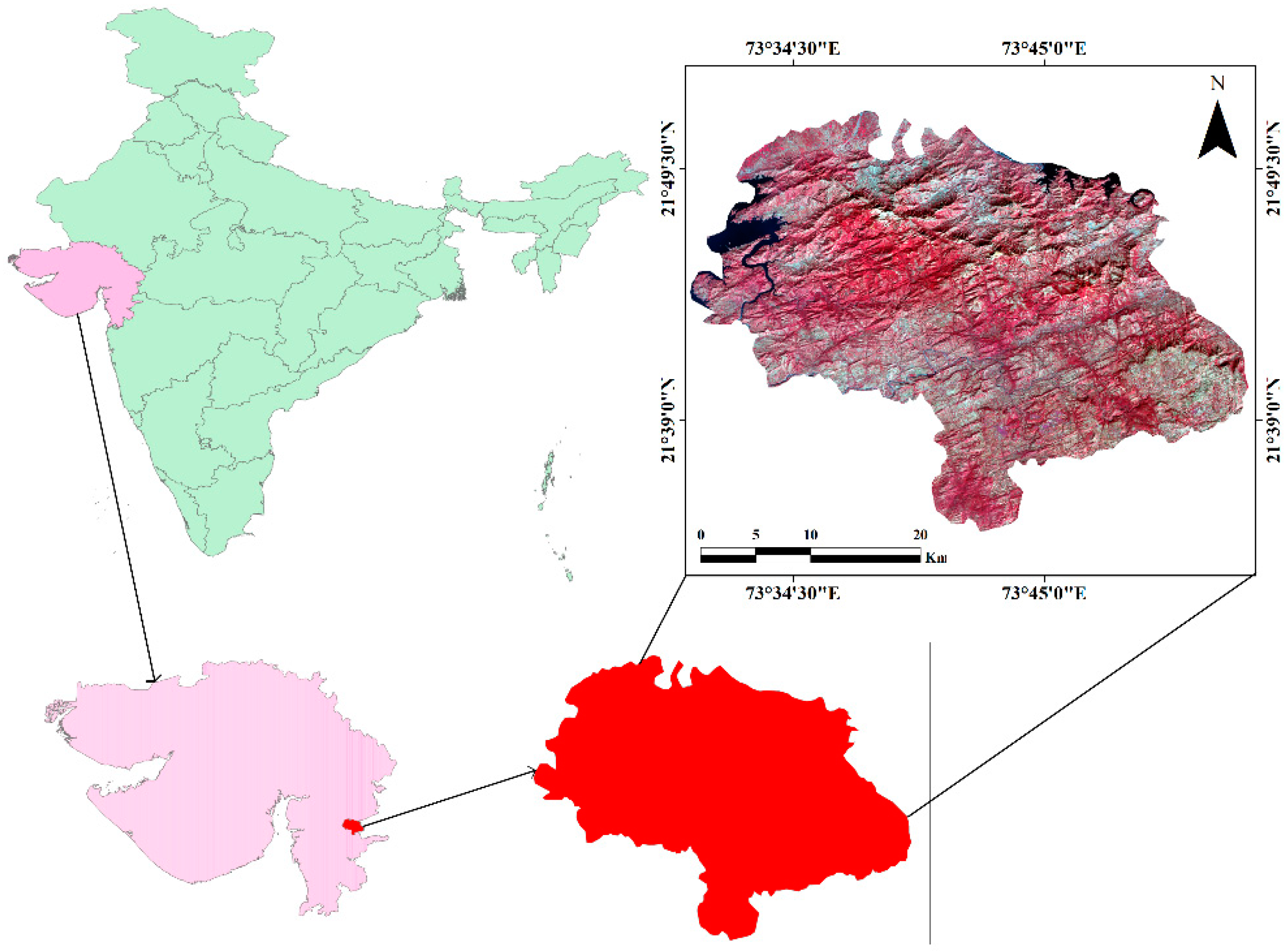
2.1. Study Area

The study area selected is the Shoolpaneshwar Wildlife Sanctuary (SWS), a protected forest area located in the Western Satpura Range south of the Narmada River, Narmada District, Gujarat State, India (Figure 1). The sanctuary was established in the year 1989 and covers 607.71 km2 geographical area. It extends from 21° 03′ N to 21° 59′ N latitude to 73° 05′ E to 74° 10′ E longitude, at an altitude of 800 to 900 m above Mean Sea Level (MSL) [60]. Two important irrigation projects, namely Sardar Sarovar and Karjan dams are based in the sanctuary. The study area comprises of mixed dry deciduous forest, riverine forest, few pockets of moist teak forest, agricultural fields, and two water reservoirs. SWS is considered to be one of the thickest forest in the state, with naturally protected regions that support the regional biota [61]. Most of the forest is covered with Tectona grandis L. and Dendrocalamus strictus [62] and the distribution of mixed species is also high within the forest. Most of the rainfall in the study area, commences with southwest monsoon in mid-June and extends till mid-October. The daily average temperature of the area in the summer (March to May) reaches 43 °C and reduces to 10 °C in winter (November–February). The SWS region is important for the support of its tribal population, regional catchment, species diversity and wildlife.

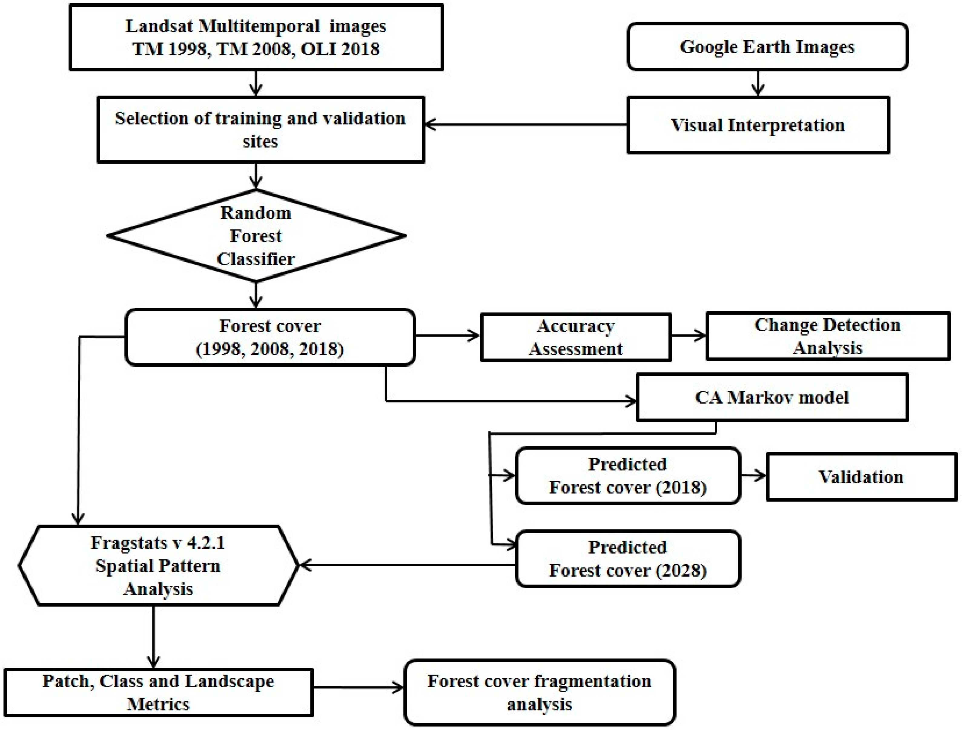
2.2. Datasets and Methodology

2.2.1. Satellite Data Acquisition & Pre-Processing

The satellite images with a spatial resolution of 30 m from Landsat 5 TM for the year 1998 and 2008 and from Landsat 8 OLI for the year 2018 were downloaded from Earth Explorer (https://earthexplorer.usgs.gov/). To minimize the haziness in the images, the dark pixel subtraction technique was applied [63,64]. Georeferencing of the images was carried out using UTM projection and WGS 84 datum and nearest neighborhood resampling method. Area under the SWS was extracted using the subset utility of the ENVI 5.1. These satellite images were used for the preparation of forest cover maps.

2.2.2. Forest Cover Classification

To perform the forest cover classification, a widely used and stable Random Forest classification algorithm was implemented in the present study. The Random Forest Classifier was applied on the pre-processed Landsat images of all 3 time intervals. This technique uses bootstrap aggregation to form an ensemble of classification and induction of tree-like classifiers. The original training sample was collected and the satellite images were used as the input parameters, the bootstrapped data helped in avoiding overfitting and generating rapid learning. The random selection of variables within the classifier also sought to minimize the correlation between the tree and it helped to decrease the error rates. This made the selection of trees from a set of multiple trees important to achieve a high accuracy within the acceptable range. The selection was feasibly achieved by optimizing the parameters within the algorithm, specifically for the classification using satellite images, setting the optimal parameter was crucial for achieving a better accuracy.
The classification was carried out using a software package in the R language. The data were trained within the random forest classifier with a multiple number of trees for the six features class. In total, six classes were established that consisted of three forest cover classes namely Dense forest, Open forest, and Degraded forest, and three non-forest cover classes namely cropland, bareland, and waterbody. For classification, the training samples for the different forest and non-forest classes were collected by visual interpretation of reference satellite and google earth images, and thereafter, the accuracy assessment was carried out using 30 training samples for each class.

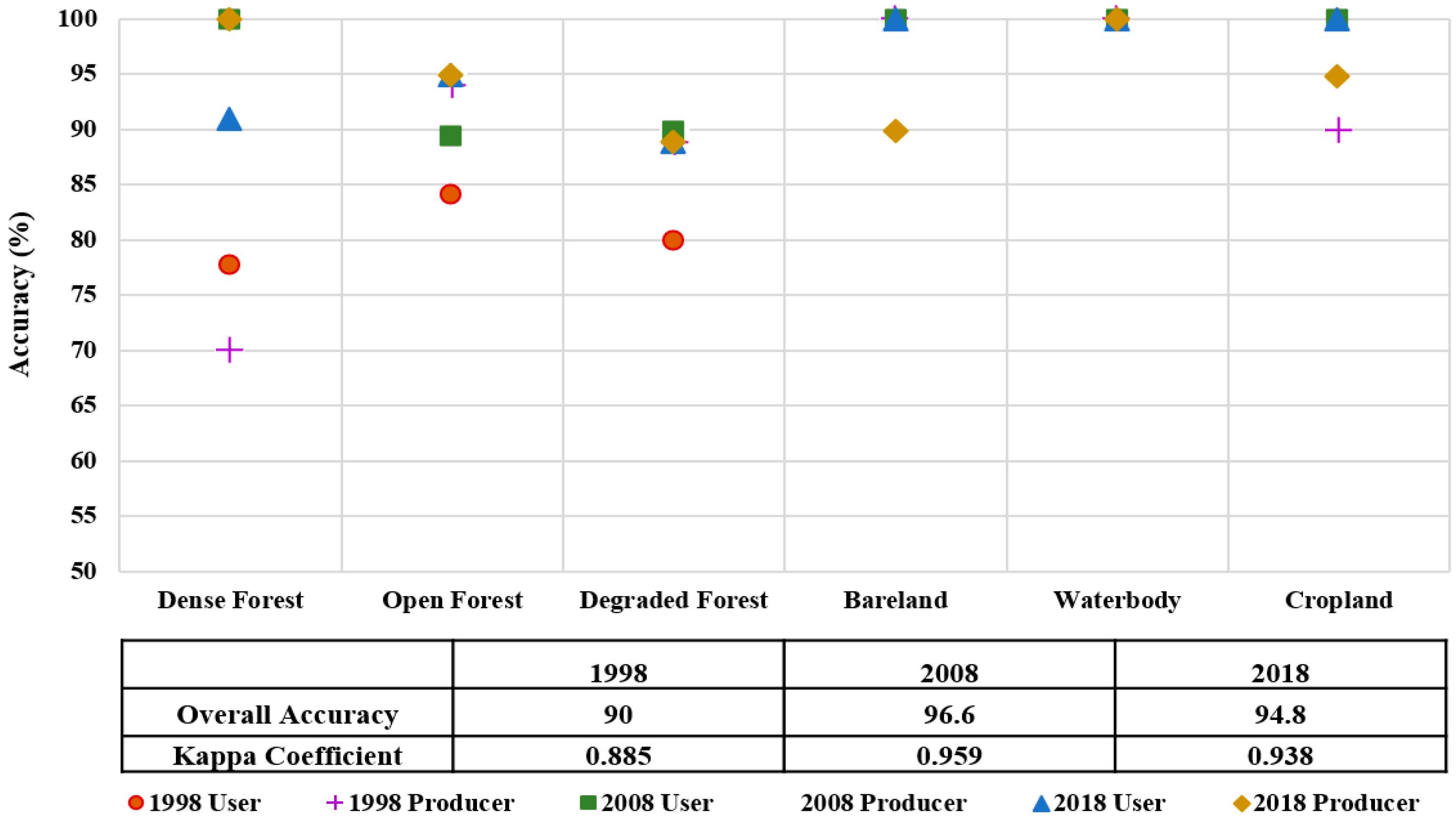
2.2.3. Accuracy Assessment

Accuracy assessment of the classified images for the year 1998, 2008, and 2018 was carried out using four statistical accuracy measures. These included the overall accuracy, errors of commission (user’s accuracy), errors of omission (producer’s accuracy), and the Kappa coefficient. A total of 30 random points for each class were considered for checking the accuracy of the thematic maps produced from the random forest technique. Ratio of the total correctly classified pixels and the total number of pixels in the error matrix provided the overall accuracy. Overall accuracy inclined to overestimate classification accuracy since it did not incorporate the proportion of agreement between datasets [65]. Producer’s accuracy indicates the probability of the reference pixel being correctly classified. User’s accuracy indicates the probability of the classified pixel of map that actually represents that class on the ground [63,66]. The Kappa coefficient incorporates the off-diagonal elements as a product of the row and column of the error matrix. This controls the chance for an agreement by removing the proportion of agreement that is expected to occur by chance [67,68]. Three temporal classified images of Landsat were compared to delineate the change in forest cover that would give status of deforestation in the study area. Temporal forest cover change analysis was subjected to the CA Markov Chain integrated modeling technique to predict the forest cover scenario for the year 2028.

2.2.4. CA-Markov Chain

In order to predict the forest cover for year 2028, CA Markov Chain was performed using the IDRISI GIS Analysis software. The CA Markov model is mainly used to simulate the spatial and temporal changes between two different land covers/forest cover, and it can generate a transitional matrix to predict future changes [69]. A cellular automata works on the concept of proximity analysis in which it examines the neighboring pixels, the transitional probability matrix determines the possibility of a pixel to convert into other class. In the present study, transitional matrix was generated for each forest cover classes that could be represented by Equation (1):
S ( t , t + 1 ) = P i j × S ( t ) S   ( t ,   t + 1 ) = P
where S(t) is system status at time t, S(t + 1) is the system status at time t + 1, Pij is the transitional probability matrix that is calculated as shown in Equation (2):
P i j = | P 1 , 1 P 1 , 2 P 1 , N P 2 , 1 P 2 , 1 P 2 , N P N , 1 P N , 2 P N , N |   ( 0 P i j 1 )
where P is the transitional probability, Pij is the probability of conversion of one classified image of time i to another classified image of time j, and PN is the probability at particular time for N number of classes. The transitional probability varied between 0 and 1. The transition was estimated by using the contiguity filter of 5 × 5 pixels, which was used to define the suitability of the neighboring pixels. The standard contiguity filter used in the present study is shown in Equation (3).
C o n t i g u i t y F i l t e r ( 5 × 5 ) = [ 0 0 1 0 0 0 1 1 1 0 1 1 1 1 1 0 1 1 1 0 0 0 1 0 0 ]
In the present study, classified Landsat images from year 1998, 2008, and 2018 are used as input parameters in the CA Markov chain model to generate a transition probability matrix to further predict the scenario for 2028. The CA Markov validation was performed using the classified image of 2018 with the predicted 2018 image, in order to evaluate the performance of the model. Four indicators, kappa for no ability (κno), standard kappa (κstandard), kappa for location (κlocation), and kappa for location strata (klocationstrata) were derived to find out the accuracy of the prediction results.

2.2.5. Fragmentation Analysis

Quantification of the forest fragmentation was carried out using the Raster version of the FRAGSTATS spatial pattern analysis software (ver.4.2.1) [70]. The changes in forest cover classes of the SWS throughout time were delineated at patch, class, and landscape levels. Quantification and comparison of the spatial configuration of forest fragments were based on the following set of metrics, selected after going through different forest fragmentation studies [71,72]. These metrics are said to be sensitive to dissection of forests and hence were used for investigating fragmentation within SWS. The selected metrics are explained in Table 1.
The brief methodology adopted in the present study is depicted in the flow chart (Figure 2) and the details of it’s implementation are provided below.

3. Results and Discussion

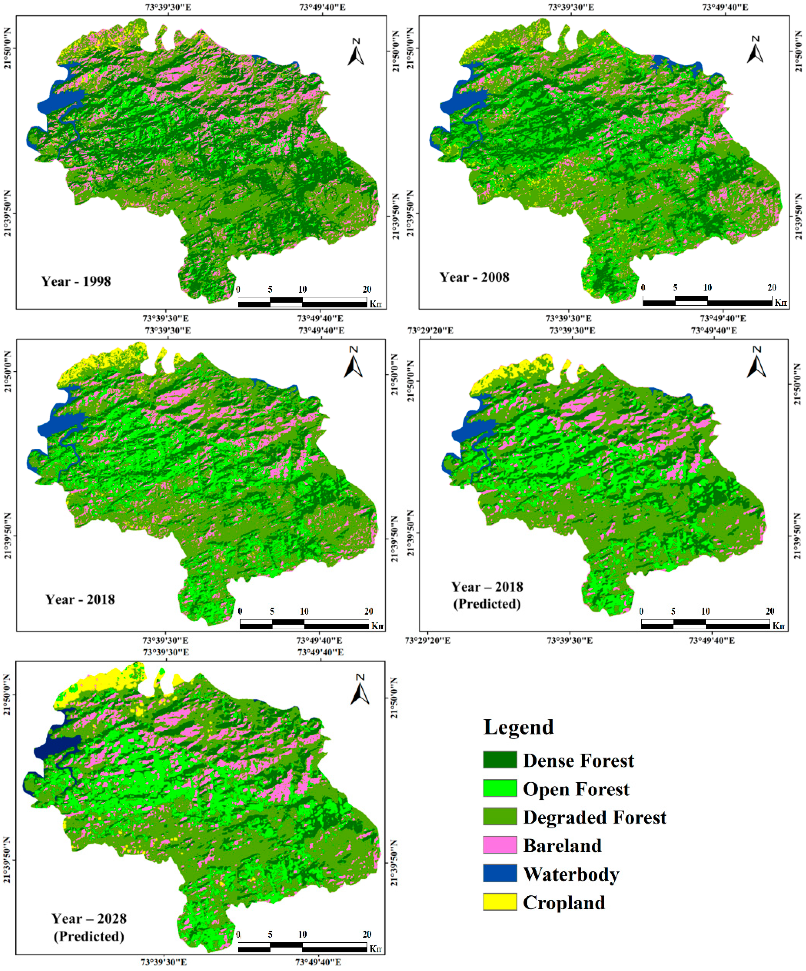
3.1. Spatiotemporal Forest Cover Classification and Accuracy Assessment

Spatiotemporal forest cover classified images for years 1998, 2008, 2018 were generated using random forest algorithm. Figure 3 shows the generated forest cover maps. User’s and Producer’s accuracies along with overall accuracy and kappa coefficient for all 1998, 2008, and 2018 are provided in Figure 4. User’s accuracy corresponds to the error of commission that was calculated by dividing the correctly classified pixel by training pixel, the producer’s accuracy corresponds to the error of omission, which was calculated by dividing the correctly classified pixels to the total number of pixel in particular class, and the overall accuracy was calculated by dividing the total number of correctly classified pixels with total reference pixels. Overall accuracy for the forest cover classification was 90.0% for 1998, 96.6% for 2008, and 94.8 % for 2018, and the Kappa coefficient was 88.5%, 95.9%, and 93.8%, respectively. In terms of producer’s accuracy for 1998, the lowest values of the producer’s accuracy (70%) and user’s accuracy (77%) corresponded to dense forest. For the classification of 2008 forest cover map, all classes showed user’s and producer’s accuracies over 89%, exhibiting accurate classification. In terms of user’s accuracy of 2018 forest cover map, all classes were over 88%, again indicating a good classification. This indicated the appropriateness of the classified Landsat images for an effective and reliable change detection analysis and prediction modeling, using the CA-Markov algorithm.

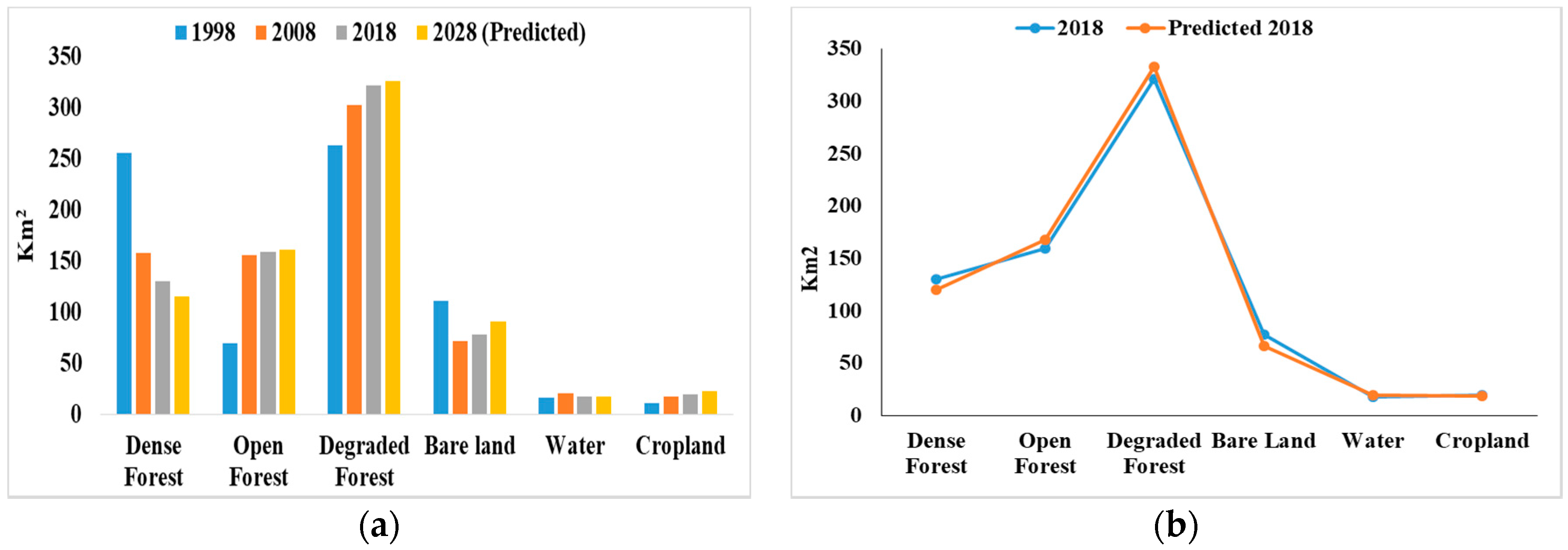
3.2. Forest Cover Modeling Using CA-Markov and Validation

CA-Markov simulated forest cover maps for the year 2018 and 2028 are shown in Figure 3. Figure 5a provides a summary of the probability matrix for forest cover conversions for all classes in SWS that occurred between 1998 and 2008. This matrix was used for generating predicted forest cover map of 2018. Figure 5b shows the transition probability matrix for time period between 2008 and 2018, which was then used for predicting future forest cover in the year 2028. Validation of the CA-Markov simulated maps was carried out by comparing predicted forest cover maps of the year 2018 with the real random forest 2018 classified forest cover map. Statistics of different classes produced using the predicted 2018 forest cover map and observed forest cover map were comparable (Figure 6b). This validated the CA-Markov generated forest cover maps, thereby, proving its effectiveness and exhibiting the predictive power of the model in predicting 2028 scenario of the forest in the SWS. Very strong predictive tools are generally considered to have accuracies of about 80% [73]. The 80% Kstandard value verified the accuracy of this model. For testing the overall accuracy of the model, the Kno value was considered as an effective alternative to Kstandard (Pontius Jr, 2000). Overall performance of the model in predicting forest cover map was quite satisfactory. This was reflected from its Kno, which was estimated 81%. The model was also capable of providing a reasonable representation of location, which was shown by its Klocation value, i.e., 81%. Additionally, visual interpretation of the results highlighted the effectiveness of the model. After investigating the predictive ability of an Integrated-Markov Chain change model, it was used to simulate 2028 forest cover map of the SWS.
The probability transition matrices for year 1998–2008 and 2008–2018 are shown in Figure 5, the probability varied from 0 to 1; represented in the form of circles. The size of the circle represents the amount of data, i.e., bigger the circle higher the number of data it holds whereas the color representation shows the class-wise probability transition. The class-wise transition within three different time period showed an interesting result. When transition of open forest into dense forest was observed, the transition probability was very low in 1998–2008. Nevertheless, the transition probability increased significantly between 2008–2018, which showed a positive change with respect to the ecosystem recovery. In case of transition of degraded forest to bare land, the probability was very low in 1998–2008 but it drastically increased between 2008–2018, which showed that the overall transition of SWS between 1998–2018 was mixed with respect to the regional ecosystem.

3.3. Change Detection Analysis

Area statistics for the random forest classification for the year 1998, 2008, 2018, and 2028 (predicted) are provided in Figure 6a. The results of class dynamics showed 38.45%, equivalent to 98.2 km2 and 17.46%, equivalent to 27.58 km2 decrease in the dense forest of SWS from period 1998 to 2008 and period 2008 to 2018, respectively. Predicted scenario of dense forest for the year 2028 showed a reduction of 11.38%, i.e., 14.83 km2 in dense forest. In 1998, dense forest occupied 34.98% of the study area, which then reduced to 21.57% and 17.8% in the year 2008 and 2018, respectively. The area under dense forest was further predicted to be decreased and it was expected to occupy 15.77%, i.e., 115.50 km2 of the study area in the year 2028. Area statistics of multi-temporal analysis exhibited a significant degradation in dense forest of SWS over the period of three decades. Area under open forest depicted a high increase of 124.4%, i.e., 86.17 km2 from the year 1998 to 2008. From year 2008 to 2018, a minor increase of 2.3%, i.e., 3.78 km2 was observed. Very small increment of around 1% was further predicted in the year 2028. Dense patches of the SWS forests were converted to open forest. Degraded forests in the study area were observed to be gradually increased. Increase of 15.3% of degraded area was observed during time period between 1998 to 2008, and 6.1% increase from the year 2008 to 2018 was noted. A minor increase of 0.1% was predicted from the year 2018 to the year 2028. Analysis of non-forest cover classes showed 63.7% and 16.4% increase in cropland area from the year 1998 to 2008, and from the year 2008 to 2018, respectively. Further increment of 11.7% was predicted from year 2018 to 2028. Variations in barren land statistics was observed during the study period, while water body showed an increase during 1998–2008 and thereafter a decrease in the area occupied for 2008–2018 time period was observed. Future prediction of 2008–2028 also showed further decrease in waterbody by 24.9%.

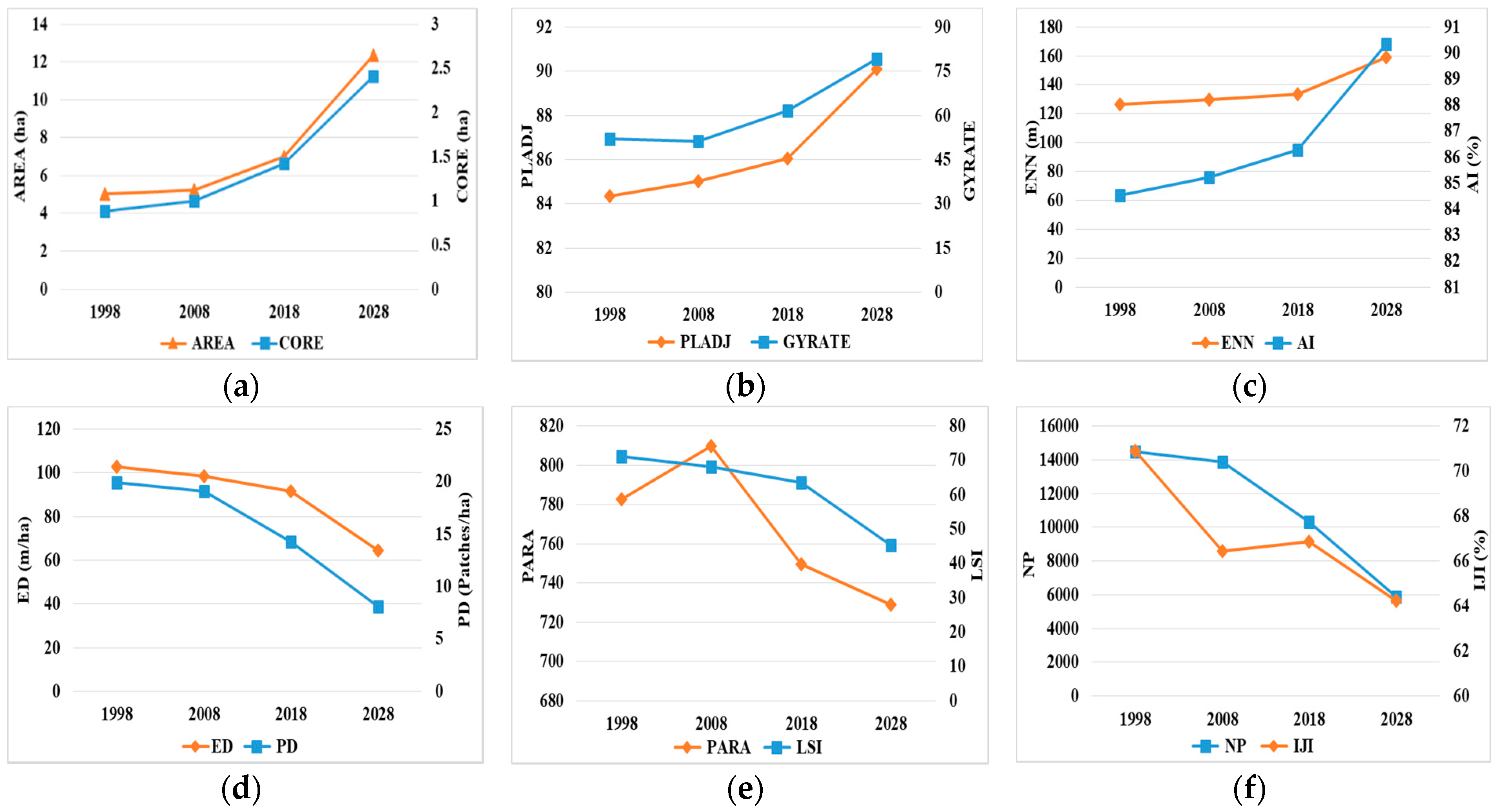
3.4. Fragmentation Analysis at Patch Level

In the SWS, significant changes were observed in the distribution of forest patches between time intervals (Table 2). Increment in number of smaller patches was one of the fundamental indicators of forest fragmentation, the reverse of which was observed in the present study area. Overall decrease in NP in of all three forest cover classes, viz. dense, open, and degraded highlights the reduction in fragmentation of the SWS. During the first period of study, i.e., 1998–2008, the total NP in dense forests showed a decline of 17.4%, where the patches got reduced from 1749 to 1444. The total NP decreased from 1444 to 1437 showed a very minor decrease of 0.5% during the second (2008–2018) period. Decrease from 1437 to 892 (37.9%) was predicted for the third period, i.e., 2018–2028.
Only 18.9 % of forest under dense vegetation was concentrated in small patches between 0 and 100 ha in the year 1998, and higher proportion of TA about 55% was covered by single fragment of size greater than 2000 ha. In 2008, TA under size category, i.e., 0–100, 100–200, 200–500 increased, and the remaining categories showed a decrease in TA. In 2018, 52.2% TA of dense forest was found in patches less than 100 ha and 33.4% dense forest in patch size of 100–200 ha. TA statistics of patches of dense forest predicted for the year 2028 forecasted the 57.3% of dense forest would be under patch size less than 100, 34.4% in 100–200 ha patch size category, and there would be no fragment greater than a patch size of 1000.
Number of patches when analyzed for open forests showed variations. Total NP increased from 3034 to 3322 (9.5%) during 1998–2008. This showed fragmentation occurrence during the first time period of 1998–2008. In second time period, i.e., from 2008-2018, total NP decreased from 3322 to 2730, which accounted for 17.8% decrease in open forests. This pointed to a control in fragmentation during this period. NP in 2028 was predicted to decrease from 2730 to 1415, i.e., a 48.2% decrease, again indicating decrease in fragmentation. Gain in smaller patches ranging between 0–100 ha was observed during 1998–2008, where the NP increased from 3031 to 3295. In 1998, 93% of the open forest area was concentrated in small patches between 0 and 100 ha; the remaining forest area occurred in isolated patches of larger than 100 ha and less than 200 ha. In 2008, 52.6% TA of open forest were observed to have a patch size less than 100, 32.1% TA was with patch size 100–200 ha, and only three fragments exceeded the patch size of 200 ha. In 2018, 28.8% TA occupied category of patch size 0–100 and 1 patch covering 28.8% TA of open forests was bigger than 2000 ha. Prediction of 2028 fragmentation status showed an increase in TA (41%), with a patch size greater than 2000 ha.
Decrease in total NP under degraded forest cover class from 3029 to 2549 (15.5% decline) was observed during 1998–2008. Time period 2008–2018 showed a 5% decrease in NP of degraded forests. Considerably a higher decrease in NP was predicted between time periods 2018–2028. In 1998, the highest TA (37.3%) was occupied by two patches with size greater than 2000 ha. Three fragments with size bigger than 2000 ha occupied the highest proportions of TA in 2008 and 2018. In 2028, TA was again predicted to be the highest, i.e., 60.3% in the same category of patch size consisting 3 fragments. In SWS, the fragmentation analysis at patch level using two metrics, namely TA and NP, showed an overall reduction in fragmentation. This emphasized that the forest at the wildlife sanctuary was monitored to a great extent, which controlled the forest fragmentation.

3.5. Fragmentation Analysis at Class Level

Class level fragmentation analysis of forest cover classes over multi-temporal scale, when carried out using twelve metrics namely NP, GYRATE, PARA, PD, AI, IJI, NLSI, CLUMPY, CONTIG, ED, CORE, and ENN, showed a decline in forest fragmentation in the SWS (Figure 7). As discussed in patch level analysis, NP in dense and degraded forests decreased from the year 1998 to 2018 and was predicted to further decrease in 2028, as per the fragmentation result of the CA-Markov simulated map. Fragmentation was observed in open classes during the time interval 1998–2008, as reflected from the increase in NP, which seemed to be monitored later, as indicated by the decreased NP from 2008–2018. Fragmentation was forecasted to be further decreased from 2018–2028.
GYRATE was said to be inversely related to forest fragmentation. Our analysis of three time-intervals showed a rise in GYRATE values in all forest cover classes over a period of time. Higher PARA values were an indicator of fragmentation. A decrease in PARA values was observed in all three forest covers, except during 1998–2008 where the PARA showed increasing values. A decreasing trend in PD of dense forests was observed where the values decreased from 2.41 to 1.98 from the year 1998 to 2018 and was predicted to reduce to 0.68 in 2028. In degraded forests, PD also decreased gradually. In open forests, PD increased from 4.18 to 4.57 in from 1998–2008 and then value decreased to 3.76 in 2018. In 2028, it would reduce to 1.08. AI showed an ascending trend, indicating a lowering in fragmentation. Variations were observed in IJI estimates. NLSI again showed a declining trend in all forest cover classes from year 1998 to 2028, and CLUMPY showed a rise in its value, except during 1998–2008, where higher values were observed in year 2008 in dense forests. Other parameters viz. CONTIG, ENN, and CORE also indicated a reduction in fragmentation, which was indicated from their increased values from the year 1998 to 2018. Values of these metrics were predicted to further rise from 2018–2028. ED showed an inverse relation with fragmentation. The values of ED showed a decreasing trend from year 1998 to 2008 in three forest cover classes, with the exception of open forest.
Overall analysis exhibited a lowering of fragmentation, as highlighted from a descending trend in quantitative estimates of the metrics viz. NP, PARA, PD, IJI, NLSI, and ED, and an ascending trend in the metrics viz. GYRATE, AI, CLUMPY, ENN, CONTIG, and CORE, with slight variations.

3.6. Fragmentation Analysis at Landscape Level

The focus of the study since remained on forest fragmentation so landscape level analysis in SWS was restricted to three forest cover classes, namely dense forest, open forest, and degraded forest. Figure 8 shows trend analysis of different landscape metrics. A gradual decrease in NP, PD, ED, and LSI was noted. PARA and IJI also showed an overall decrease with slight variations. Increase in values of metrics namely GYRATE, CORE, ENN, AREA, AI, and PLADJ was observed. Overall results depict a decline in fragmentation from year 1998 to 2018. Trend analysis of these metrics also indicated a further decrease in the fragmentation in 2028.
Fragmentation is considered to be an important procedure within the worldwide ongoing process of landscape degradation, driven by environmental changes and socioeconomic processes like global change, urbanization, and improvement of transport infrastructure. Many human activities are said to be responsible for this degradation. Diverse macroeconomic, demographic, technological, institutional, and political factors are the driving factors for these human activities responsible for forest degradation [74,75]. Fragmentation analysis results at all three patch, class, and landscape levels highlight the decrease in SWS fragmentation. This indicates that fragmentation is well controlled in the sanctuary, which is due to certain management practices adopted in the area. The primary reasons for forest degradation in India are well noted by the Gujarat state government. These include critical livelihood–forest linkage of a large forest dependent, exploitation of forest products beyond its carrying capacity due to demand and supply gap, frequent forest fires, uncontrolled and unrestrained over-grazing, illegal felling, and forest land diversion to some other land uses [76]. Even certain past forest management practices that enhance degradation were noted. These factors can decimate the forest–biodiversity to a great extent, and thus can degrade the forests. The state has already taken significant steps to monitor forests. These include in and ex-situ conservation, afforestation/plantations, social/community/farm forestry, Joint Forest Management (JFM), addressing issues involved in sub-sectors like grasslands and mangroves, creation of protected areas, improvement in policies, legal provisions, etc. SWS is one of the Hot Spots of Biodiversity and is thus considered to be under management and conservation sites, as per The Biological Biodiversity Act, 2002, Section 37. Status-quo on the conservation of SWS is well maintained by the Gujarat State. Introduction of two important forest management practices, namely Narmada Dam Catchment Area Treatment and JFM [77,78] considerably improved the conservation of biodiversity in the forests of Narmada forests. This makes SWS a better protected area and thus could be the reason for the reduction in fragmentation in SWS. The results of the present study are also supported by a previous study, where low fragmentation was observed in the sanctuary [79]. Such results were also seen in a study carried out in other national parks, where less fragmentation was recorded in the park when compared to non-park areas [80].

4. Conclusions

Random forest classifier was applied on the Landsat images to delineate spatiotemporal forest cover changes during 1998, 2008, and 2018, in SWS. Meanwhile, the CA-Markov Chain integrated hybrid model was used to predict a future forest cover scenario. The present analysis was based on the assumption that the situation in the future would remain unchanged and the trend would remain similar to what was estimated, but this was not the case all the time. The transition probability matrix generated between 1998–2008 and 2008–2018 showed an unstable shift in some of the variable transitions, therefore, a rigorous training of models was done while predicting future scenarios. Transition probability matrix derived from the classified images of SWS during 1998, 2008, and 2018 showed the variation in different classes with time, and the transition matrix was further used to predict forest cover status in the year 2018 and 2028. This predicted image of 2018 was compared with a classified forest cover image of 2018 for validating the predictive model. The forest cover maps of year 1998, 2008, 2018, and the predicted map of 2028 was subjected to the Fragstats software, for checking the past and future fragmentation scenario in SWS. Overall, the results of fragmentation statistics clearly depicted a reduction in fragmentation in the forest areas of SWS during the year 1998, 2008, and 2018. There was a trend of forest degradation, which was also observed in the present study. It showed the forest degradation is occurring but the rate of forest degradation is gradually decreasing, and with the reduction in forest fragments it can be seen as a positive sign for the regional ecosystem. As shown in the transition probability matrix, open forests are increasing with the time and barelands are gradually being converting into open forest and croplands. The fragmentation is forecasted to further decrease in 2028, based on the present analysis. A framework for the future conservation practices could be implemented by using the present study results. To our knowledge, forest officials of SWS are aware of this need and have successfully implemented management and conservation practices in the sanctuary. This could be a good implication for forest officials of other sanctuaries in the country and other countries. These conservation initiatives of the officials could be considered to be the key reason for making the sanctuary a better protected area, due to which a decline in fragmentation could be observed.

Author Contributions

Conceptualization, Prashant K. Srivastava and G. Sandhya Kiran; Data curation, Ramandeep Kaur M. Malhi, and Akash Anand; Formal analysis, Ramandeep Kaur M. Malhi, and Akash Anand; Funding acquisition, Christos Chalkias; Investigation, Prashant K. Srivastava, and George P. Petropoulos; Methodology, Prashant K. Srivastava and Ramandeep Kaur M. Malhi; Project administration, Prashant K. Srivastava; Resources, Prashant K. Srivastava and George P. Petropoulos; Software, Akash Anand; Supervision, Prashant K. Srivastava; Visualization, and Akash Anand; Writing—original draft, Ramandeep Kaur M. Malhi and Akash Anand; Writing—review & editing, Prashant K. Srivastava, G. Sandhya Kiran, George P. Petropoulos, and Christos Chalkias. All authors have read and agreed to the published version of the manuscript.

Funding

Authors would like to thank the Science and Engineering Research Board, Department of Science and Technology for the financial support to the first author to carry out this research work under National Postdoctoral Fellowship scheme (PDF/2017/002620).

Acknowledgments

Authors are thankful to Ministry of Environment, Forest, and Climate Change and Gujarat Forest Department for providing necessary approval to perform sampling in the sanctuary. A warm thanks is also extended to local forest officials for helping with the sampling. We would also like to thank the anonymous reviewers for their useful feedback that resulted in improving the manuscript.

Conflicts of Interest

The authors declare no conflict of interest.

References

  1. Kiran, G.S.; Malhi, R.K.M. Economic valuation of forest soils. Curr. Sci. 2011, 100, 396–399. [Google Scholar]
  2. Lewis, S.L.; Edwards, D.P.; Galbraith, D. Increasing human dominance of tropical forests. Science 2015, 349, 827–832. [Google Scholar] [CrossRef]
  3. Fahrig, L. Effects of habitat fragmentation on biodiversity. Annu. Rev. Ecol. Evol. Syst. 2003, 34, 487–515. [Google Scholar] [CrossRef] [Green Version]
  4. Forman, R.T.; Godron, M. Landscape Ecology; John Wiley & Sons: New York, NY, USA, 1986; Volume 4, pp. 22–28. [Google Scholar]
  5. Haila, Y. Islands and fragments. In Maintaining Biodiversity in Forest Ecosystems; Cambridge University Press: Cambridge, UK, 1999. [Google Scholar]
  6. Anand, A.; Malhi, R.K.M.; Pandey, P.C.; Petropoulos, G.P.; Pavlides, A.; Sharma, J.K.; Srivastava, P.K. Use of Hyperion for Mangrove Forest Carbon Stock Assessment in Bhitarkanika Forest Reserve: A Contribution Towards Blue Carbon Initiative. Remote Sens. 2020, 12, 597. [Google Scholar] [CrossRef] [Green Version]
  7. Pandey, P.C.; Anand, A.; Srivastava, P.K. Spatial distribution of mangrove forest species and biomass assessment using field inventory and earth observation hyperspectral data. Biodivers. Conserv. 2019, 28, 2143–2162. [Google Scholar] [CrossRef]
  8. Foley, J.A.; DeFries, R.; Asner, G.P.; Barford, C.; Bonan, G.; Carpenter, S.R.; Chapin, F.S.; Coe, M.T.; Daily, G.C.; Gibbs, H.K. Global consequences of land use. Science 2005, 309, 570–574. [Google Scholar] [CrossRef] [Green Version]
  9. Wade, T.G.; Riitters, K.H.; Wickham, J.D.; Jones, K.B. Distribution and causes of global forest fragmentation. Conserv. Ecol. 2003, 7, 7. [Google Scholar] [CrossRef]
  10. Gamfeldt, L.; Snäll, T.; Bagchi, R.; Jonsson, M.; Gustafsson, L.; Kjellander, P.; Ruiz-Jaen, M.C.; Fröberg, M.; Stendahl, J.; Philipson, C.D. Higher levels of multiple ecosystem services are found in forests with more tree species. Nat. Commun. 2013, 4, 1–8. [Google Scholar] [CrossRef]
  11. Marchetti, M.; Sallustio, L.; Ottaviano, M.; Barbati, A.; Corona, P.; Tognetti, R.; Zavattero, L.; Capotorti, G. Carbon sequestration by forests in the National Parks of Italy. Plant Biosyst. Int. J. Deal. All Asp. Plant Biol. 2012, 146, 1001–1011. [Google Scholar] [CrossRef]
  12. Benitez-Malvido, J. Impact of forest fragmentation on seedling abundance in a tropical rain forest. Conserv. Biol. 1998, 12, 380–389. [Google Scholar] [CrossRef]
  13. Laurance, W.F.; Nascimento, H.E.; Laurance, S.G.; Andrade, A.; Ewers, R.M.; Harms, K.E.; Luizao, R.C.; Ribeiro, J.E. Habitat fragmentation, variable edge effects, and the landscape-divergence hypothesis. PLoS ONE 2007, 2, e1017. [Google Scholar] [CrossRef] [PubMed]
  14. Loynl, R.H.; McAlpine, C. Spatial Patterns and Fragmentation: Indicators for Conserving Biodiversity in Forest. Criteria Indic. Sustain. For. Manag. 2001, 7, 391. [Google Scholar]
  15. Azevedo, J.; Perera, A.H.; Pinto, M.A. Forest Landscapes and Global Change: Challenges for Research and Management; Springer: Berlin, Germany, 2014. [Google Scholar]
  16. Rochelle, J.A.; Lehmann, L.A.; Wisniewski, J. Forest Fragmentation: Wildlife and Management Implications; Brill: Leiden, The Netherlands, 1999. [Google Scholar]
  17. Forman, R. Land Mosaics: The ecology of landscapes and regions (1995). In The Ecological Design and Planning Reader; IslandPress: Washington, DC, USA, 2014; pp. 217–234. [Google Scholar]
  18. Harris, L.D.; Harris, L.D. The Fragmented Forest: Island Biogeography Theory and the Preservation of Biotic Diversity; University of Chicago press: Chicago, IL, USA, 1984. [Google Scholar]
  19. Hill, J.; Curran, P. Species composition in fragmented forests: Conservation implications of changing forest area. Appl. Geogr. 2001, 21, 157–174. [Google Scholar] [CrossRef]
  20. Pontius, R.G., Jr. Comparison of categorical maps. Photogramm. Eng. Remote Sens. 2000, 66, 1011–1016. [Google Scholar]
  21. Achard, F.; Hansen, M.C. Global Forest Monitoring from Earth Observation; CRC Press: Boca Raton, FL, USA, 2012. [Google Scholar]
  22. Dougherty, E.R.; Newell, J.T.; Pelz, J.B. Morphological texture-based maximum-likelihood pixel classification based on local granulometric moments. Pattern Recognit. 1992, 25, 1181–1198. [Google Scholar] [CrossRef]
  23. Specht, D.F. A general regression neural network. IEEE Trans. Neural Netw. 1991, 2, 568–576. [Google Scholar] [CrossRef] [Green Version]
  24. Menard, S. Applied Logistic Regression Analysis; Sage: Thousand Oaks, CA, USA, 2002; Volume 106. [Google Scholar]
  25. Huang, C.; Davis, L.; Townshend, J. An assessment of support vector machines for land cover classification. Int. J. Remote Sens. 2002, 23, 725–749. [Google Scholar] [CrossRef]
  26. Kamusoko, C.; Aniya, M.; Adi, B.; Manjoro, M. Rural sustainability under threat in Zimbabwe–simulation of future land use/cover changes in the Bindura district based on the Markov-cellular automata model. Appl. Geogr. 2009, 29, 435–447. [Google Scholar] [CrossRef]
  27. Kantakumar, L.N.; Neelamsetti, P. Multi-temporal land use classification using hybrid approach. Egypt. J. Remote Sens. Space Sci. 2015, 18, 289–295. [Google Scholar] [CrossRef] [Green Version]
  28. Breiman, L. Random forests. Mach. Learn. 2001, 45, 5–32. [Google Scholar] [CrossRef] [Green Version]
  29. Feng, Q.; Liu, J.; Gong, J. UAV remote sensing for urban vegetation mapping using random forest and texture analysis. Remote Sens. 2015, 7, 1074–1094. [Google Scholar] [CrossRef] [Green Version]
  30. Kamusoko, C.; Gamba, J. Simulating urban growth using a Random Forest-Cellular Automata (RF-CA) model. ISPRS Int. J. Geo-Inf. 2015, 4, 447–470. [Google Scholar] [CrossRef]
  31. Rodriguez, J.D.; Perez, A.; Lozano, J.A. Sensitivity analysis of k-fold cross validation in prediction error estimation. IEEE Trans. Pattern Anal. Mach. Intell. 2009, 32, 569–575. [Google Scholar] [CrossRef] [PubMed]
  32. Ruiz Hernandez, I.E.; Shi, W. A Random Forests classification method for urban land-use mapping integrating spatial metrics and texture analysis. Int. J. Remote Sens. 2018, 39, 1175–1198. [Google Scholar] [CrossRef]
  33. More, A.; Rana, D.P. Review of random forest classification techniques to resolve data imbalance. In Proceedings of the 2017 1st International Conference on Intelligent Systems and Information Management (ICISIM), Maharashtra, India, 5–6 October 2007; pp. 72–78. [Google Scholar]
  34. Ranjan, A.K.; Anand, A.; Vallisree, S.; Singh, R.K. LU/LC change detection and forest degradation analysis in Dalma wildlife sanctuary using 3S technology: A case study in Jamshedpur-India. Aims Geosci. 2016, 2, 273–285. [Google Scholar] [CrossRef]
  35. Mishra, V.N.; Prasad, R.; Kumar, P.; Gupta, D.K.; Srivastava, P.K. Dual-polarimetric C-band SAR data for land use/land cover classification by incorporating textural information. Environ. Earth Sci. 2017, 76, 26. [Google Scholar] [CrossRef]
  36. Ranjan, A.K.; Anand, A.; Kumar, P.B.S.; Verma, S.K.; Murmu, L. Prediction of Land Surface Temperature within Sun City Jodhpur (Rajasthan) in India Using Integration of Artificial Neural Network and Geoinformatics Technology. Asian J. Geoinform. 2018, 17, 14–23. [Google Scholar]
  37. Wolfram, S. Cellular Automata and Complexity: Collected Papers; CRC Press: Boca Raton, FL, USA, 2018. [Google Scholar]
  38. Suzuki, J. A Markov chain analysis on simple genetic algorithms. IEEE Trans. Syst. ManCybern. 1995, 25, 655–659. [Google Scholar] [CrossRef]
  39. Verhagen, P. Case Studies in Archaeological Predictive Modelling; Amsterdam University Press: Amsterdam, The Netherlands, 2007; Volume 14. [Google Scholar]
  40. Halmy, M.W.A.; Gessler, P.E.; Hicke, J.A.; Salem, B.B. Land use/land cover change detection and prediction in the north-western coastal desert of Egypt using Markov-CA. Appl. Geogr. 2015, 63, 101–112. [Google Scholar] [CrossRef]
  41. Vázquez-Quintero, G.; Solís-Moreno, R.; Pompa-García, M.; Villarreal-Guerrero, F.; Pinedo-Alvarez, C.; Pinedo-Alvarez, A. Detection and projection of forest changes by using the Markov Chain Model and cellular automata. Sustainability 2016, 8, 236. [Google Scholar] [CrossRef] [Green Version]
  42. Cabral, P.; Zamyatin, A. Markov processes in modeling land use and land cover changes in Sintra-Cascais, Portugal. Dyna 2009, 76, 191–198. [Google Scholar]
  43. Glenn-Lewin, D.C.; Peet, R.K.; Veblen, T.T. Plant Succession: Theory and Prediction; Springer Science & Business Media: Berlin/Heidelberg, Germany, 1992; Volume 11. [Google Scholar]
  44. Hu, Z.; Lo, C. Modeling urban growth in Atlanta using logistic regression. Comput. Environ. Urban Syst. 2007, 31, 667–688. [Google Scholar] [CrossRef]
  45. Kucsicsa, G.; Popovici, E.-A.; Bălteanu, D.; Dumitraşcu, M.; Grigorescu, I.; Mitrică, B. Assessing the Potential Future Forest-Cover Change in Romania, Predicted Using a Scenario-Based Modelling. Environ. Model. Assess. 2019, 1–21. [Google Scholar] [CrossRef]
  46. Lepš, J. Mathematical modelling of ecological succesion—A review. Folia Geobot. Et Phytotaxon. 1988, 23, 79–94. [Google Scholar] [CrossRef]
  47. Liu, Y. Modelling Urban Development with Geographical Information Systems and Cellular Automata; CRC Press: Boca Raton, FL, USA, 2008. [Google Scholar]
  48. Guan, D.; Li, H.; Inohae, T.; Su, W.; Nagaie, T.; Hokao, K. Modeling urban land use change by the integration of cellular automaton and Markov model. Ecol. Model. 2011, 222, 3761–3772. [Google Scholar] [CrossRef]
  49. Keshtkar, H.; Voigt, W. A spatiotemporal analysis of landscape change using an integrated Markov chain and cellular automata models. Model. Earth Syst. Environ. 2016, 2, 10. [Google Scholar] [CrossRef] [Green Version]
  50. Mitsova, D.; Shuster, W.; Wang, X. A cellular automata model of land cover change to integrate urban growth with open space conservation. Landsc. Urban Plan. 2011, 99, 141–153. [Google Scholar] [CrossRef]
  51. Subedi, P.; Subedi, K.; Thapa, B. Application of a hybrid cellular automaton–Markov (CA-Markov) model in land-use change prediction: A case study of Saddle Creek Drainage Basin, Florida. Appl. Ecol. Environ. Sci. 2013, 1, 126–132. [Google Scholar] [CrossRef] [Green Version]
  52. Çakir, G.; Sivrikaya, F.; Keleş, S. Forest cover change and fragmentation using Landsat data in Maçka State Forest Enterprise in Turkey. Environ. Monit. Assess. 2008, 137, 51–66. [Google Scholar] [CrossRef]
  53. Ojoyi, M.; Odindi, J.; Mutanga, O.; Abdel-Rahman, E. Analysing fragmentation in vulnerable biodiversity hotspots in Tanzania from 1975 to 2012 using remote sensing and fragstats. Nat. Conserv. 2016, 16, 19. [Google Scholar]
  54. Midha, N.; Mathur, P. Assessment of forest fragmentation in the conservation priority Dudhwa landscape, India using FRAGSTATS computed class level metrics. J. Indian Soc. Remote Sens. 2010, 38, 487–500. [Google Scholar] [CrossRef]
  55. Singh, S.K.; Pandey, A.C.; Singh, D. Land use fragmentation analysis using remote sensing and Fragstats. In Remote Sensing Applications in Environmental Research; Springer: Berlin, Germany, 2014; pp. 151–176. [Google Scholar]
  56. Carranza, M.L.; Frate, L.; Acosta, A.T.; Hoyos, L.; Ricotta, C.; Cabido, M. Measuring forest fragmentation using multitemporal remotely sensed data: Three decades of change in the dry Chaco. Eur. J. Remote Sens. 2014, 47, 793–804. [Google Scholar] [CrossRef]
  57. Linh, N.; Erasmi, S.; Kappas, M. Quantifying land use/cover change and landscape fragmentation in Danang City, Vietnam: 1979–2009. Int. Arch. Photogramm. Remote Sens. Spat. Inf. Sci. 2012, 39, B8. [Google Scholar] [CrossRef] [Green Version]
  58. Singh, S.K.; Srivastava, P.K.; Szabó, S.; Petropoulos, G.P.; Gupta, M.; Islam, T. Landscape transform and spatial metrics for mapping spatiotemporal land cover dynamics using Earth Observation data-sets. Geocarto Int. 2017, 32, 113–127. [Google Scholar] [CrossRef] [Green Version]
  59. Tapia-Armijos, M.F.; Homeier, J.; Espinosa, C.I.; Leuschner, C.; de la Cruz, M. Deforestation and forest fragmentation in South Ecuador since the 1970s–losing a hotspot of biodiversity. PLoS ONE 2015, 10, e0133701. [Google Scholar] [CrossRef] [Green Version]
  60. Malhi, R.K.M.; Anand, A.; Mudaliar, A.N.; Pandey, P.C.; Srivastava, P.K.; Sandhya Kiran, G. Synergetic use of in situ and hyperspectral data for mapping species diversity and above ground biomass in Shoolpaneshwar Wildlife Sanctuary, Gujarat. Trop. Ecol. 2020, 61, 106–115. [Google Scholar] [CrossRef]
  61. Christian, B.; Krishnayya, N. Discrimination of floor cover of dry deciduous forest using Hyperion (EO-1) data. J. Indian Soc. Remote Sens. 2008, 36, 137–148. [Google Scholar] [CrossRef]
  62. Pradeepkumar, G.; Prathapasenan, G. Floristic Diversity and Biotic Pressure in Shoolpaneshwar Wildlife Sanctuary, Gujarat. In Chapter in Air Pollut. Dev. What Cost? Daya Publishing House: Delhi, India, 2003; pp. 148–159. [Google Scholar]
  63. Lillesand, T.; Kiefer, R.W.; Chipman, J. Remote Sensing and Image Interpretation; John Wiley & Sons: New York, NY, USA, 2015. [Google Scholar]
  64. Srivastava, P.K.; Malhi, R.K.M.; Pandey, P.C.; Anand, A.; Singh, P.; Pandey, M.K.; Gupta, A. Revisiting hyperspectral remote sensing: Origin, processing, applications and way forward. In Hyperspectral Remote Sensing; Elsevier: Amsterdam, The Netherlands, 2020; pp. 3–21. [Google Scholar]
  65. Congalton, R.G.; Mead, R.A. A quantitative method to test for consistency and correctness in photointerpretation. Photogramm. Eng. Remote Sens. 1983, 49, 69–74. [Google Scholar]
  66. Anand, A.; Singh, S.K.; Kanga, S. Estimating the change in Forest Cover Density and Predicting NDVI for West Singhbhum using Linear Regression. Int. J. Environ. Rehabil. Conserv. 2018, 9, 193–203. [Google Scholar]
  67. Cohen, J. A coefficient of agreement for nominal scales. Educ. Psychol. Meas. 1960, 20, 37–46. [Google Scholar] [CrossRef]
  68. Yuan, F.; Bauer, M.E.; Heinert, N.J.; Holden, G.R. Multi-level land cover mapping of the Twin Cities (Minnesota) metropolitan area with multi-seasonal Landsat TM/ETM+ data. Geocarto Int. 2005, 20, 5–13. [Google Scholar] [CrossRef]
  69. Arsanjani, J.J.; Helbich, M.; Kainz, W.; Boloorani, A.D. Integration of logistic regression, Markov chain and cellular automata models to simulate urban expansion. Int. J. Appl. Earth Obs. Geoinf. 2013, 21, 265–275. [Google Scholar] [CrossRef]
  70. McGarigal, K. FRAGSTATS: Spatial Pattern Analysis Program for Categorical Maps. Computer Software Program Produced by the Authors at the University of Massachusetts, Amherst. Available online: http://www.umass.edu/landeco/research/fragstats/fragstats.html (accessed on 9 July 2020).
  71. Armenteras, D.; Gast, F.; Villareal, H. Andean forest fragmentation and the representativeness of protected natural areas in the eastern Andes, Colombia. Biol. Conserv. 2003, 113, 245–256. [Google Scholar] [CrossRef]
  72. Imbernon, J.; Branthomme, A. Characterization of landscape patterns of deforestation in tropical rain forests. Int. J. Remote Sens. 2001, 22, 1753–1765. [Google Scholar] [CrossRef]
  73. Araya, Y.H.; Cabral, P. Analysis and modeling of urban land cover change in Setúbal and Sesimbra, Portugal. Remote Sens. 2010, 2, 1549–1563. [Google Scholar] [CrossRef] [Green Version]
  74. Stanturf, J.A.; Palik, B.J.; Dumroese, R.K. Contemporary forest restoration: A review emphasizing function. For. Ecol. Manag. 2014, 331, 292–323. [Google Scholar] [CrossRef]
  75. Vásquez-Grandón, A.; Donoso, P.J.; Gerding, V. Forest degradation: When is a forest degraded? Forests 2018, 9, 726. [Google Scholar] [CrossRef] [Green Version]
  76. Davidar, P.; Sahoo, S.; Mammen, P.C.; Acharya, P.; Puyravaud, J.-P.; Arjunan, M.; Garrigues, J.P.; Roessingh, K. Assessing the extent and causes of forest degradation in India: Where do we stand? Biol. Conserv. 2010, 143, 2937–2944. [Google Scholar] [CrossRef]
  77. Kiran, G.S.; Baria, P.; Malhi, R.K.M.; Revdandekar, A.V.; Mudaliar, A.N.; Joshi, U.B.; Shah, K.A. Site Suitability Analysis for JFM Plantation Sites using Geo-Spatial Techniques. Int. J. Adv. Remote Sens. GIS 2015, 4, 920–930. [Google Scholar] [CrossRef]
  78. Malhi, R.K.M.; Kiran, G.S. Impact of Joint Forest Management strategy on fertility of forest soils. Bull. Environ. Sci. Res. 2013, 2, 7–11. [Google Scholar]
  79. Bhatt, G.; Kushwaha, S.; Nandy, S.; Bargali, K.; Nagar, P.; Tadvi, D. Analysis of fragmentation and disturbance regimes in south Gujarat forests, India. Trop. Ecol. 2015, 56, 275–288. [Google Scholar]
  80. Kayiranga, A.; Kurban, A.; Ndayisaba, F.; Nahayo, L.; Karamage, F.; Ablekim, A.; Li, H.; Ilniyaz, O. Monitoring forest cover change and fragmentation using remote sensing and landscape metrics in Nyungwe-Kibira park. J. Geosci. Environ. Prot. 2016, 4, 13–33. [Google Scholar] [CrossRef] [Green Version]
Figure 1. Map depicting the study area (shown in red color).
Ijgi 09 00530 g001
Figure 2. Flowchart depicting the methodology used in this study.
Ijgi 09 00530 g002
Figure 3. Forest cover maps of year 1998, 2008, 2018, 2018 (Predicted) and 2028 (Predicted).
Ijgi 09 00530 g003
Figure 4. Accuracy assessment for random forest classification for the year 1998, 2008, and 2018.
Ijgi 09 00530 g004
Figure 5. (a) Probability transition matrix for 1998–08. (b) Probability transition matrix for 2008–2018.
Ijgi 09 00530 g005
Figure 6. (a) Area Statistics (km2) of the Land Use and Land Cover (LULC) classes for the years 1998, 2008, 2018, and predicted 2028. (b) Area Statistics (km2) of 2018 versus predicted 2018.
Ijgi 09 00530 g006
Figure 7. Different class level fragmentation metrics plotted over multi-temporal scale for different forest cover classes (a) Number of Patches (NP), (b) Radius of Gyration (GYRATE), (c) Perimeter Area Ratio (PARA), (d) Patch Density (PD), (e) Aggregation Index (AI), (f) Interspersion Juxtaposition Index (IJI), (g) Normalized Land Shape Index (NLSI), (h) Clumpiness (CLUMPY), (i) Contiguity Index (CONTIG), (j) Edge Density (ED), (k) Euclidean Nearest Neighbour (ENN), and (l) Core Area (CORE).
Ijgi 09 00530 g007
Figure 8. Different landscape level fragmentation metrics plotted over multitemporal scale for forest cover. (a) Mean Area (AREA) and Core Area (CORE), (b) Proportion of Like Adjacencies (PLADJ) and Radius of Gyration (GYRATE), (c) Euclidean Nearest Neighbour (ENN) and Aggregation Index (AI), (d)Edge Density (ED) and Patch Density (PD), (e) Perimeter Area Ratio (PARA) and Landscape Shape Index (LSI), and (f) Number of Patches (NP) and Interspersion Juxtaposition Index (IJI).
Ijgi 09 00530 g008
Table 1. Description of metrics computed in the present study at different levels.
MetricUnit/
Range
Level of AnalysisFormulaExplanation
PCL
Total Area
(TA)
ha TA = A(1/10000)Area of each patch or class or landscape
Mean Area (AREA)ha AREA = aij(1/10000)The average size of the patches of the corresponding forest type.
Smaller mean patch size indicates more fragmented forest
Core Area
(CORE)
ha C O R E = a i j c ( 1 10000 ) It is the area in the patches which is within the depth of edge distance from the patch perimeter of the corresponding forest type.
The core area decreases with the increase in fragmentation.
No of Patches
(NP)
-niIt is the total number of patches of corresponding patch class.
More the patch more will be the fragmentation.
Patch Density
(PD)
Patches/100 ha PD =(ni/A)*(10000)*(100)It is simply the total number of patches per 100 hectares of area.
Higher the patch density higher will be the fragmentation.
Edge Density
(ED)
m/ha ED = ( k = 1 m e i k / A ) 10000 It is the sum of edge segment length of corresponding patch type divided by the total patch area.
A high ED value represents a higher degree of fragmentation. When the whole landscape is composed of only one patch, the ED value will approach zero.
Radius of Gyration (GYRATE) 0 GYRATE = k = 1 z h i j r It is the mean distance between cell and the centroid of the patch.
Increase in Gyrate indicates increase in patch size that indicates reduction in fragmentation
Perimeter Area Ratio
(PARA)
>0 P A R A = P i j a i j It is the ratio of patch perimeter and area.
Lower the PARA higher will be the fragmentation and vice versa.
Contiguity Index (CONTIG)0–1 C O N T I G = [ r = 0 n C i j r a i j ] 1 v 1 It is the spatial interconnections between neighboring pixels. It varies from 0 to 1, where 0 indicates single pixel patch whereas higher value indicates more patch interconnection.
Higher the CONTIG lower will be the fragmentation
Interspersion Juxtaposition Index (IJI)% I J I = i = 1 m k = i + 1 m [ ( e i k E ) l n ( e i k E ) | ] l n ( 0.5 [ m ( m 1 ) ] ) 100 IJI defines the interspersion of a given patch by estimating the observed interspersion over maximum possible interspersion.
Lower the interspersion lower will be the fragmentation.
Proportion of Like Adjacencies (PLADJ)% P L A D J = ( g i j k = 1 m g i k ) ( 100 ) PLADJ calculates the number of like adjacencies divided by the total cell adjacencies, it also involves the focal class. It varies from 0 to 100, where 0 represents the patch with maximum disaggregation.
Lower the PLADJ higher will be the fragmentation.
Aggregation Index (AI)% A I = [ g i i m a x g i i ] ( 100 ) It is the like adjacencies of a particular class divided by the maximum possible like adjacencies of that particular class. It ranges from 0 to 100, where 0 indicates more disaggregation. Lower the AI more is the fragmentation.
Clumpiness (CLUMPY)−1 to 1 C L U M P Y = [ G i P i 1 P i ]
Where, G i = ( g i i n = 1 m g i i m i n ( e i ) )
It is the proportion of like adjacencies (Gi) minus proportion of landscape of focal class.
Lower value of CLUMPY indicates higher fragmentation whereas higher value shows less fragmentation.
Normalized Land Shape Index (NLSI) 0 N L S I 1 N L S I = e i m i n e i m a x e i m i n e i It is the total perimeter of a corresponding class minus the minimum observed perimeter divided by the difference of maximum and minimum perimeter of class.
Lower the NLSI value lower will be the fragmentation and vice versa.
Euclidean Nearest Neighbor
(ENN)
m E N N = j = 1 n X i j n i It is the sum of all corresponding patch type divided by the total number of same patch type.
Lower the ENN value higher will be the fragmentation and vice versa
Landscape Shape Index
(LSI)
L S I 1 L S I = e i m i n e i It is the total edge length divided by the minimum possible length of class edge.
The lowest value 1 shows a very compact patch that is less fragmentation whereas higher the LSI value higher will be the fragmentation.
where A = total landscape area (m2); aij =area of patch ij; aijc = core area of patch ij based on specific edge depth (in meters); ni =total number of patches; m = total edge length; eik = total edge length including landscape boundary of patch type i; hijr = distance between cell ijr (located within patch ij) and centroid of patch ij; z =total number of cells in patch ij; Pij = perimeter of patch ij; aij = area of patch ij; cijr = contiguity for pixel r in patch ij; v = sum of template value; eik = total edge length in landscape between patch I and k; E or ei = total length of edge in landscape; gii = number of like adjacencies between pixels of patch type i; gik = number of adjacencies between pixels of patch type i and k; max gii = maximum number of gii; Pi = proportion of the landscape occupied by patch type i; ei = total length of edge of class i; and minei = minimum total length of edge of class i.
Table 2. Patch level analysis of Total Area (TA) and No of Pataches (NP) for different forest covers classes.
Dense Forest
Patch SizeTA (ha)NP
19982008201820281998200820182028
0–1004839.574244.496800.586616.98173314261412872
100–5002856.153274.654357.353980.1611122319
500–10001195.023157.11786.15953.192411
1000–20002572.381483.021089.1802110
>200014,148.723629.07001100
Open Forest
Patch SizeTA (ha)NP
19982008201820281998200820182028
0–1006454.628174.256653.074901.043031329527131399
100–500471.784989.243761.462470.233241511
500–100002379.96921.152105.10314
1000–200000000000
>2000004580.646598.440011
Degraded Forest
Patch SizeTA (ha)NP
19982008201820281998200820182028
0–1006621.575418.725846.584975.23002253423971358
100–5003443.222618.732263.054774.3217101115
500–10004262.491401.031336.952163.516223
1000–20002156.3102962.081706.942021
>20009804.9620,867.6720,245.520,717.642333

