Assessment of Interventions in Fuel Management Zones Using Remote Sensing

Abstract

Every year, wildfires strike the Portuguese territory and are a concern for public entities and the population. To prevent a wildfire progression and minimize its impact, Fuel Management Zones (FMZs) have been stipulated, by law, around buildings, settlements, along national roads, and other infrastructures. FMZs require monitoring of the vegetation condition to promptly proceed with the maintenance and cleaning of these zones. To improve FMZ monitoring, this paper proposes the use of satellite images, such as the Sentinel-1 and Sentinel-2, along with vegetation indices and extracted temporal characteristics (max, min, mean and standard deviation) associated with the vegetation within and outside the FMZs and to determine if they were treated. These characteristics feed machine-learning algorithms, such as XGBoost, Support Vector Machines, K-nearest neighbors and Random Forest. The results show that it is possible to detect an intervention in an FMZ with high accuracy, namely with an F1-score ranging from 90% up to 94% and a Kappa ranging from 0.80 up to 0.89.

1. Introduction

Every year in Portugal thousands of hectares of forest are consumed by fires causing environmental, infrastructural, and personal damages [1]. With the purpose to minimize the damages caused by fires, the Portuguese government established Fuel Management Zones (FMZs), which are zones where the vegetation has to be treated, meaning the removal or partially removal of vegetation, to protect different types of infrastructures and to also work as strategic points for fighting fires [2,3]. Since responsibility of the treatment of FMZs falls onto who owns a certain terrain, like like citizens, private entities, as well as counties, actively monitoring the treatments of FMZs is critical. The National Republican Guard is responsible for the monitoring of the FMZs.

FMZs cover a large part of the Portuguese territory forming a three-level network: Primary Network, Secondary Network, and Tertiary Network. The primary network is defined at the district level, while secondary and tertiary networks are defined at the municipal and local levels. Furthermore, the interventions made in these zones are classified as follows: Fuel Reduction Zones (FRZs) and Fuel Interruption Zones (FIZs). FRZs are characterized by the removal of surface vegetation and the cutting of trees to create a separation between cups. FIZs consist of the total removal of all types of vegetation within the defined range [4].

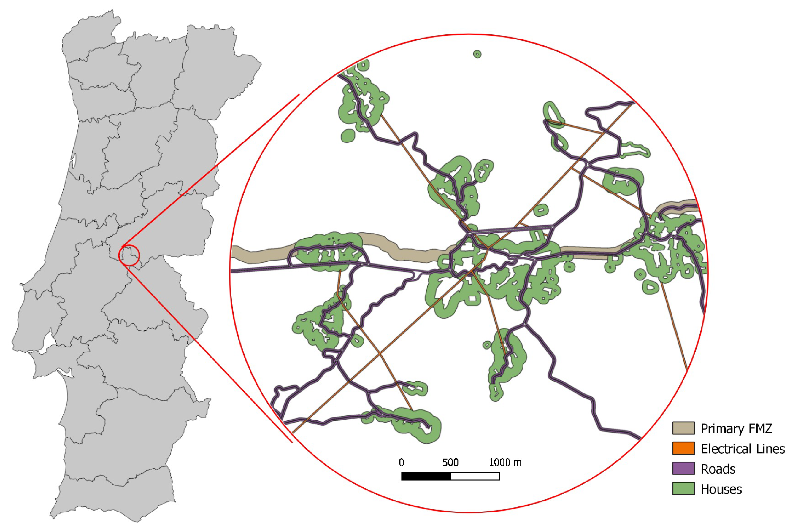
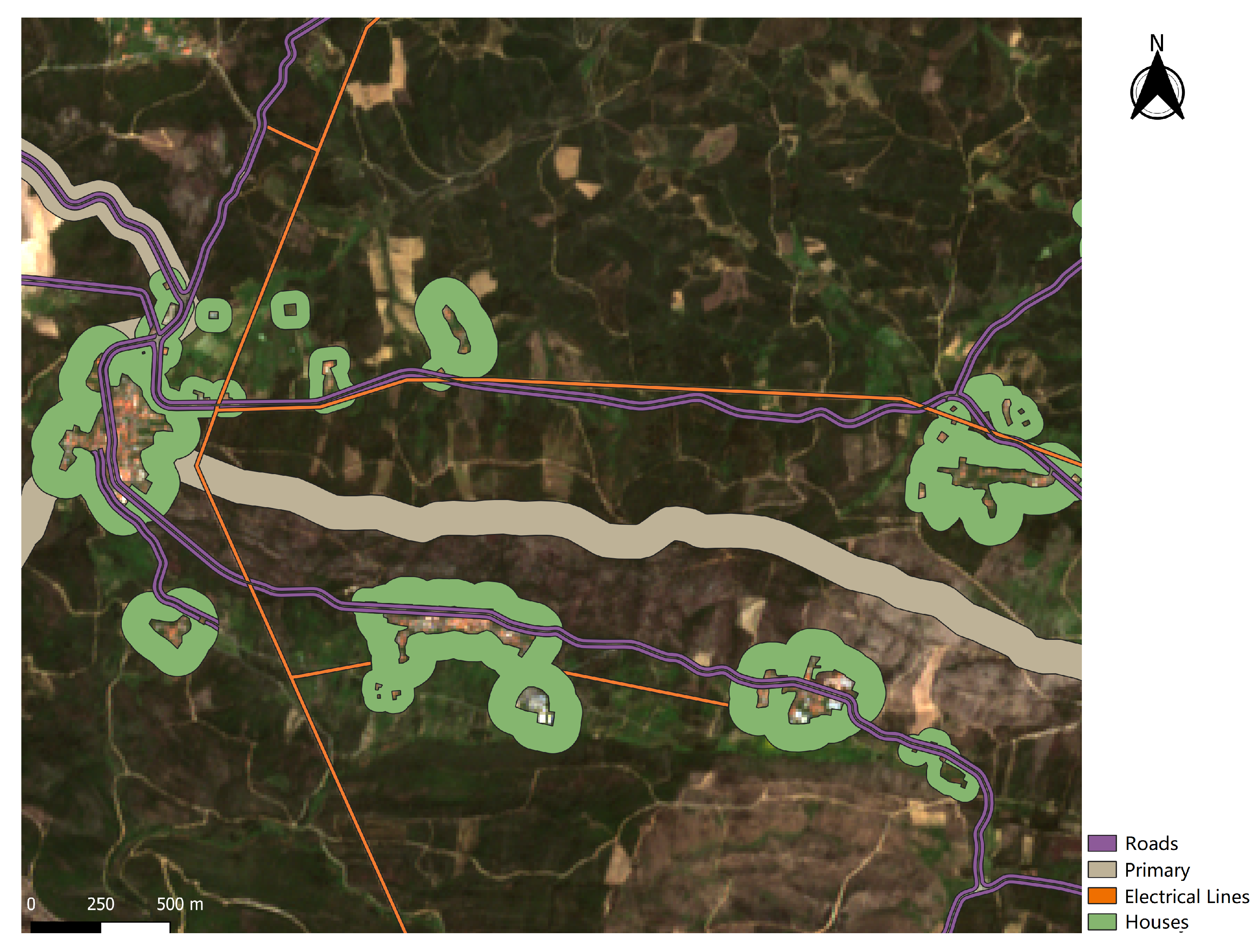
The primary FMZ covers a large part of the Portuguese territory, dividing it into plots with a size between 500 ha and 10,000 ha. This network consists of 125 m wide strips. Beyond reducing the area traveled by forest fires, these strips are also an auxiliary element in the planning of firefighting, since this network is built in strategic areas. The secondary and tertiary FMZs are defined around roads, tracks, powerlines, railways, and settlements. These networks are part of the Municipal Plan for the Defense of Forests Against Fires. The strips created along roads, tracks, and railways are of the FIZ type. Strips around individual houses and settlements are also FIZ types with the addition that the canopy of trees must be more than 5 m apart from the dwellings. High and medium voltage electrical distribution lines and natural gas transmission lines are also part of these networks.

Since FMZs can have huge extensions (thousands of hectares), it can be difficult for the authorities to monitor these zones and identify which ones require intervention. The existence of automatic or semi-automatic processes that allow the identification of FMZs that were treated, could help the monitoring process, speeding up the detection of zones in need of intervention, thus allowing timely maintenance and increasing the overall protection against forest fires. The use of machine- learning methods applied to remote sensing for large scale geographical analysis is common [5,6,7,8]. The Institute for the Conservation of Nature and Forests (ICNF) maintains the geographical information about FMZs and makes this information publicly available. Combining this information with publicly available satellite imagery from satellites such as Sentinel-1 and Sentinel-2 that that capture images with resolutions up to 10 by 10 m, opens up the possibility of integrating new methods that use remote detection in the FMZs monitoring process.

The FMZs must be treated every year so that during the fire season the vegetation inside is as reduced as possible so that these zones fulfill their purpose. The high extent of these zones and the fact that a large part of the FMZs intersects with private land can hinder the cleaning process and generate discontinuities in the treated areas of the FMZs. These factors make monitoring the treated zones or detecting zones in need of intervention a complex problem.

Although forest fires are a serious problem, there has not been extensive research into the monitoring process of FMZs. In [9], the Normalized Difference Vegetation Index (NDVI) was used, along with geographic information of roads and agricultural fields, to identify FMZs. In a different context, the work of [10] compared the precision of three digital surface models to estimate the elevation of the terrain in the areas that concern FMZs, in a northern part of Greece.

There are several approaches regarding crop and vegetation monitoring and biomass estimation that can be used as a basis to build a robust solution for the monitoring of FMZs. Some studies in which the focus is to classify types of crops [8,11,12], others that classify tree species in forest areas [8], and also a more comprehensive classification approaches that focus on distinguishing different types of land cover (e.g., forest, urban, agricultural areas, etc.) [5,13,14]. Some studies only use data from satellite bands directly [5,8], although in most cases vegetation indices are used as indicators of vegetation characteristics. Some works use time series to extract more information about vegetation [11,14,15]. The use of time series has already shown better results in the classification of vegetation and land cover than the use of data referring to only one date [14,16].

There are also some studies in which the dimension and the characteristics of the analyzed areas are similar to those of FMZs [17,18]. Immitzer et al. [8] classified the vegetation in an agricultural area and a forest area using the Random Forests. In the agricultural area, 8 types of crops were classified and in the forest area 6 species of trees. Two approaches were compared: pixel-based and object-based, and it was observed that in the forest area the object-based approach obtained better results. Clevers et al. [17] used Sentinel-2 data and vegetation indices to analyze areas similar to the size of FMZs, with 30 by 30 m. Also using the same data type Rozenstein et al. [19] found that there is a strong correlation ($R^2=0.94$) between the NDVI and the water consumption of that plant, which may be helpful when analyzing the state of vegetation in an FMZ. Other studies attempt to estimate the production of a given crop following indicators such as Leaf Area Index (LAI) and vegetation indices [20,21]. Setiyono et al. [21] used Synthetic Aperture Radar (SAR) data from Sentinel-1 and multispectral data from the MODIS satellite to estimate rice production, compared to data obtained in the field, obtaining errors of less than 10%. Castillo et al. [22] used Sentinel-2, Sentinel-1, and elevation data, along with some vegetation indices to estimate the amount of biomass present in mangrove forests in the Philippines. The results showed a correlation between the levels of biomass with some vegetation indices and the LAI.

All the information presented in these works serves as a knowledge base to establish an adequate strategy to carry out the classification of interventions and monitoring the state of vegetation in FMZs. This paper presents an automated machine- learning approach that leverages time series to detect if an FMZs was treated or not using open satellite data at a resolution of 10 by 10 m. To the best of our knowledge, this is the first work that proposes a machine- learning approach to detect if the FMZs are maintained according to the law. Machine learning combined with remote sensing can accelerate the process of monitoring these FMZs which otherwise would be time-consuming. Furthermore, the monetary costs associated with the manual labor required to monitor the FMZs could be mitigated by using open satellite data. The contributions from this paper are as follows: (1) a methodology for detecting interventions in FMZs is presented, which uses information about vegetation present inside and outside the FMZs. This approach can be used to analyze any FMZ type that roughly follows the specifications, dimensions, shape, and purpose; (2) a set of software tools that given the vector information about the FMZs and a set of satellite images can extract metrics from the time- series patterns, and estimate if the FMZs was or not maintained properly with a high degree of accuracy.

This paper is organized as follows: Section 2 describes the experimental processing pipeline, showing how the data was acquired and processed, how the FMZs were clustered, and how the data sets were created. Section 3 shows and compares the results by pairing multiple algorithms with different data sets. Finally, Section 4 and Section 5 presents the discussion and conclusions.

2. Materials and Methods

2.1. Study Area

The study area chosen was Mação in the Santarém district, as shown in Figure 1. This area has been hit several times by fires and has been managing FMZs for several years. The area is situated in the central part of continental Portugal (39°32′54.708″ N–8°0′17.9964″ W), and its FMZs cover an area of about 4263 ha, with 1120 ha being FMZs around roads. Along with geographic information, in vector format, about this municipality FMZs, a collaboration was established between NOVA LINCS (a Computer Science research laboratory located at the Faculty of Science and Technology of the NOVA University of Lisbon) and the city hall of Mação which provided information about the FMZs that were treated in 2018. In Figure 2 some FMZs that have been treated (white) and others that have not (red) are represented. This type of information is essential to validate the created models.

2.2. Approach Overview

To detect an intervention in an FMZ, this work proposes comparing the vegetation inside the FMZs and the vegetation in the outer areas adjacent to the FMZs, by creating buffers adjacent to the FMZs boundaries. FMZs have different dimensions (they can vary between 10 and 125 m in width), have a format that varies according to the type of FMZ and also, it is necessary to guarantee that these buffers are located on vegetation areas. The materials that are used as a base for the analysis are satellite images and the FMZs vector information.

The satellite imagery is pre-processed, and the areas of interest were cut to obtain just the data from the FMZs areas that are being analyzed. The FMZs vector information is also pre-processed and used to cut the satellite imagery. From the resulting image, several metrics are extracted and then fed into the machine- learning algorithms to make the predictions. The algorithms with the best results in the literature were used to assess which works best for the presented problem. The used algorithms are Support vector machine (SVM), Random Forest (RF), Extreme Gradient Boosting (XGBoost), and K-nearest neighbors (KNN). The performance of these algorithms will be mainly analyzed through the F1-score (Equation (1)), which reaches its max value with perfect precision and recall, and the Kappa score.

$$\text{F1-score}=2\ast \frac{precision\ast recall}{precision+recall}$$

(1)

To optimize the learning algorithms the input data was split into two sets, train and test with a 70% and 30% split. 70% of the data (train set) was used in conjunction with 5-fold cross-validation to find the best parameters for all the algorithms via random search of the algorithm’s parameters.

2.3. Satellite Data Acquisition

The used approach uses a combination of data extracted from two satellite constellations, Sentinel-1 and Sentinel-2, as well as some derived indices derived from the multispectral data: NDVI [23], Soil-Adjusted Vegetation Index (SAVI) [24], Simple Ratio (SR) [25], Inverted Red-Edge Chlorophyll Index (IRECI) [26] and Normalized Difference Water Index (NDWI) [27]. The data used in this study was extracted from ESA’s Copernicus between 30th of January 2018 and 28th of December 2018, the distribution of the images throughout the year is presented in Figure 3, with a total of 20 images for Sentinel-2, and for Sentinel-1, 30 in descending orbit and 30 in ascending orbit. For Sentinel-2 data, only images with a cloud cover percentage below 10% were considered, which were then manually checked to ensure there were no clouds over the study area.

Some Sentinel-2 satellite products only provide reflectance values at the top of the atmosphere (level 1C). This can be problematic when dealing with multi-temporal data since the composition of the atmospheric layer is not constant, and can vary depending on the time of year or even the location. This instability has an impact on the values obtained by the satellite bands and, consequently, on the vegetation indices calculated from them, especially when multi-temporal data is being used [28,29]. The tool Sen2Cor [30] was used to process Sentinel-2 level 1C data to the corrected level 2A.

For Sentinel-1, images with the product type Ground Range Detected (GRD) were used, in descending and ascending orbit with intensity values converted to Gamma0. The processing pipeline, using the ESA Sentinel Application Platform (SNAP) (ESA Sentinel Application Platform (SNAP)—http://step.esa.int/main/toolboxes/snap/—Last visited on 6 March 2020), was as follows: (1) Apply-Orbit-File; (2) Terrain-Correction; (3) LinearToFromdB.

2.4. FMZs Vector Information Processing

All FMZ types are present in a single vector file and to analyze each one of them individually it is necessary to previously separate them by their type. This separation was made in 4 types of FMZ: roads, powerlines, settlements, and primary FMZ, as presented in Figure 4. The used approach to detect if an FMZ has been treated consists of the comparison of the vegetation inside the FMZ with the vegetation outside the FMZ. To make this comparison possible, buffers that are external to the FMZ with a width of 20 m were created. The shape of the resulting polygons that represent the FMZ varies depending on its type and because of that the process to create the buffers needs to be adapted.

For powerlines, roads, and primary FMZ the process of buffer creation is similar. The final result, along with the intermediate results, are presented in Figure 5. First, take the original FMZ, Figure 5a, and apply a buffer with 20 m for each side obtaining Figure 5b. Finally, cut the original FMZ from the buffer in order to obtain only the exterior zones as presented in Figure 5c.

For FMZs surrounding houses and settlements, buffer creation is more complex, as only the buffer on the outer part of the FMZs is needed. These FMZs have a circular shape and many holes, where the actual buildings are. Applying a simple buffer creates many intersection zones inside the polygon. To solve this the processing chain presented in Figure 6 is applied. First, extract all the points belonging to the FMZ vector file and apply the Concave hull algorithm [31], as a result, the envelope of a set of points is obtained, present in Figure 6b. After applying Concave Hull, the resulting polygon is dissolved, and its holes are filled resulting in the polygon presented in Figure 6c. Finally, apply a 20 m buffer to the initial FMZ and use the dissolved polygon to cut into the buffer, resulting in only the outer buffer of the FMZ (Figure 6d).

Some faults on the final buffers can be observed in Figure 5c and Figure 6d. Road information extracted from OpenStreetMap [32] was cut into the final FMZ buffers, due to roads not being part of these FMZs. This removes unwanted buffer zones where FMZs have areas in its interior that do not belong to the FMZs (e.g., roads).

2.5. FMZs Vector Clustering

The FMZs have a large extension and to analyze them this paper proposes an object-based approach in which the FMZs were divided into sections with approximately the same dimension. Since the satellite images have a spatial resolution of 10 m, some FMZs can have a width of multiple pixels, making it difficult to compare the values of the pixels in the buffer with the ones inside the FMZ. Using an object-based approach simplifies this comparison by combining the value of multiple pixels into just one value, and comparing the two values (the buffer value with the FMZ value). The object-based approach has other benefits such as noise reduction of pixels that could have been affected by the reflectance of nearby structures. Another advantage of this approach is the decrease in the data set size, reducing the computation time of the machine- learning algorithms.

The creation of sections is done after the buffers are created so each section has information about the FMZ and the outside buffer. These sections were created using K-means [33] whose cluster results will be referred to as FMZ segments. By using K-means the segments inherit some of its properties like like creating non-hierarchical and nonoverlapping clusters in a Voronoi pattern, which creates similar-sized segments along with the extent of the FMZ. One of K-means’ drawbacks is that the number of clusters (K) must be known before running the algorithm.

The used approach goes as follows: first, transform the pixels that correspond to the interior of the FMZ and the buffer into points (Figure 7a). The K is then selected by dividing the total number of points in an FMZs with the number of wanted pixels in a single segment. For example, in the case of FMZs along roads, with a total of 208,000 points and 40 points per cluster, 5200 segments were obtained. After testing a range of numbers, 10 to 100, of points per cluster, 40 points was the value chosen to present the results and methodology of this paper. This value is the value that better represents segments of FMZs and intersects their interior and exterior. The number of points per section cannot be very low (e.g., 10), as it generates sections that do not cover the strip and its exterior buffer, nor can be too high (e.g., 100) to reduce the possibility of a section containing treated and untreated areas. After visual inspection, this value represents a balance between the resolution of the pixels, the width of the FMZs and the created buffers. Finally, to obtain the polygon that corresponds to a section, the Convex Hull algorithm is run for each cluster generated by K-Means. The result is a set of polygons with approximately the same area, which covers the entire FMZ (Figure 7b) and keeps information on which points belong to the interior and exterior of the FMZ. Examples of the final results for each FMZ type are shown in Figure 8. Please note that the FMZ type affects the overall shape of the segments.

2.6. Data Sets

Multiple characteristics were used to describe the FMZ interior and the outside buffer for each section. In addition to the satellite data, new features were extracted using the Sentinel-2 bands and Sentinel-1 polarizations. The extracted features are present in

Table 1. Calculated characteristics for each one of the satellites.

Satellite	Calculated Characteristics
Sentinel-1	VV/VH, VV-VH
Sentinel-2	NDVI, NDWI, SAVI, IRECI, SR

. For Sentinel-1 the difference and ratio between the VV and VH polarizations in both ascending and descending orbits are calculated since they have already been shown to improve classification accuracy [34]. For Sentinel-2 some vegetation indices were derived.

With these characteristics, 5 data sets were created to compare the impact of each group of characteristics in the results (

Table 2. Tested data sets and its characteristics.

Data Sets	Base Attributes
DS_ALL	NDVI, NDWI, SAVI, IRECI, SR, B02, B03, B04, B05, B06, B07, B08, B11, (VV_DESC, VH_DESC, VV-VH_DESC, VV/VH_DESC, VV_ASC, VH_ASC, VV-VH_ASC, VV/VH_ASC) *
DS_INDICES	NDVI, NDWI, SAVI, IRECI, SR, (VV_DESC, VH_DESC, VV-VH_DESC, VV/VH_DESC, VV_ASC, VH_ASC, VV-VH_ASC, VV/VH_ASC) *
DS_BAND	B02, B03, B04, B05, B06, B07, B08, B11, (VV_DESC, VH_DESC, VV-VH_DESC, VV/VH_DESC, VV_ASC, VH_ASC, VV-VH_ASC, VV/VH_ASC) *
DS_FUSION	NDVI, NDWI, B03, B04, B05, B06, B07, B08, (VV_DESC, VH_DESC, VV-VH_DESC, VV/VH_DESC, VV_ASC, VH_ASC, VV-VH_ASC, VV/VH_ASC) *
DS_SAR	VV_DESC, VH_DESC, VV-VH_DESC, VV/VH_DESC, VV_ASC, VH_ASC, VV-VH_ASC, VV/VH_ASC

* Sentinel-1 data only used in time- series analysis.

). The data set DS_ALL has all Sentinel-2 bands, vegetation indices and Sentinel-1 polarizations, data set DS_INDICES has only vegetation indices and DS_BAND has only satellite bands. The DS_FUSION was created using the red, green, red-edge and near-infrared bands, which are the bands that are used in the vegetation indices calculations, and two indices that assess different vegetation characteristics: NDVI and NDWI. Finally, the DS_SAR exclusively using Sentinel-1 data.

For each one of these characteristics, the information from the interior of the FMZ and the outer buffer was extracted. Complementing that, the difference (Equation (2)) and ratio (Equation (3)) between the outer buffer and interior FMZ was calculated for every characteristic. With this, every segment ends up with data about the buffer, FMZ, difference, and ratios.

$$di{f}_x=x_b-x_i$$

(2)

$$rati{o}_x=\frac{x_b}{x_i}$$

(3)

where $x_b$ represents buffer data and $x_i$ the FMZ data, for the characteristic x.

Multi-temporal analysis can take advantage of the multiple images extracted, as for each characteristic the difference between two consecutive dates is calculated for the whole time series (Equation (4)).

$$\mathsf{\Delta }di{f}_k=(\frac{daysToPreviousDate-maxDays}{maxDays-minDays})\ast (di{f}_{x,k}-di{f}_{x,k-1})$$

(4)

where $di{f}_{x,k}$ represents the difference between the outer buffer and the interior of the FMZ for attribute x, on date k.

In the temporal analysis, each one of these characteristics generates a temporal pattern, and from that pattern, the metrics max, min, mean, and standard deviation are extracted. These values are used as a representation of the vegetation behavior over time, for each section.

3. Results

In this section, the results for both the static analysis (one date only, Section 3.1) and temporal analysis (time-series data from 2018, Section 3.2) are presented for roads. Other types of FMZ were left out a more detailed analyses due to uncertainty and absence of ground truth. For both types of analysis, the four chosen algorithms (KNN, RF, SVM, and XGBoost) were trained on all the defined data sets. Furthermore, all experiences of temporal analysis were repeated with and without Sentinel-1 data, as this allowed the assessment of the impact that radar data has in the detection of FMZs interventions. Both the code and the data used to obtain these results are available online at https://bitbucket.org/rfafonso/fuel-management-zones-interventions/commits/cef0be1.

3.1. Static Analysis

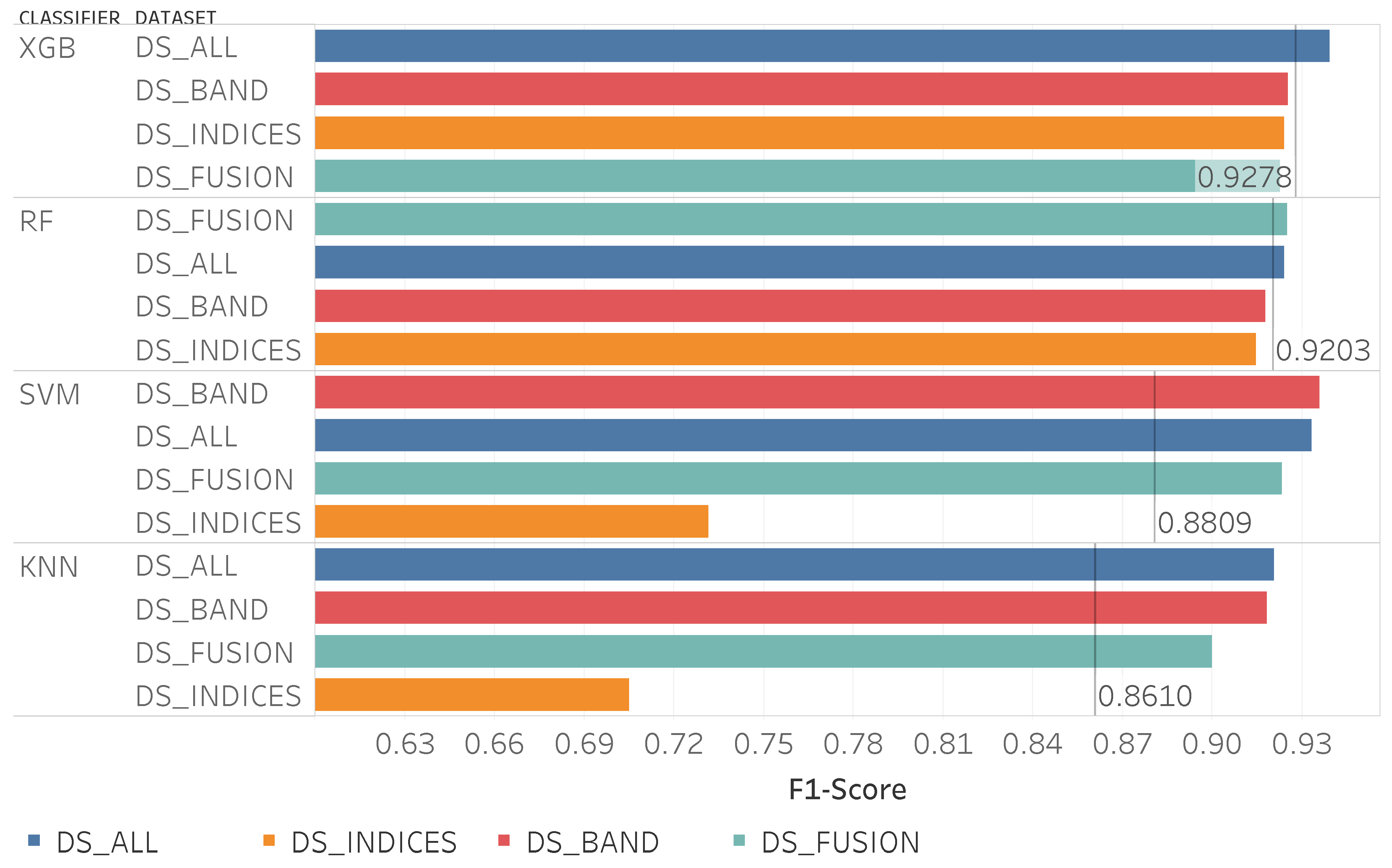
The first analysis consists of comparing different data sets using only Sentinel-2 data from just one date, 12 September, this is the date closest to our ground truth. Figure 9 shows the F1-score values for the used algorithms and the different data sets, note that the data sets are sorted by performance and by model. The RF and XGBoost were the algorithms that achieved better results, with RF reaching slightly better values.

The data set DS_ALL consistently delivered good results for all the algorithms and the best result was achieved using this data set with the RF algorithm. The data set choice, in this case, can have a great impact on the results, in some cases, it has an impact in the F1-score superior to 4%. The lowest result was obtained using the data set DS_INDICES with SVM, resulting in an F1-score of 0.83.

Analyzing in more detail the combination that generated the best results (RF using DS_ALL data set) using a confusion matrix (

Table 3. Confusion Matrix for the algorithm RF using the DS_ALL data set.

Predicted\Reference	Treated	Not Treated	Total	Precision	Recall	F1-Score
Treated	90	17	107	0.84	0.80	0.82
Not Treated	23	1257	1287	0.98	0.99	0.98
Total	112	1275
Global F1-Score (macro)	0.90
Global Kappa	0.80

) the class of “not treated” sections was the one with a higher F1-score of 0.98 and with a precision and recall of 0.98 and 0.99, respectively. The class of “treated” sections had a lower F1-score value of 0.82.

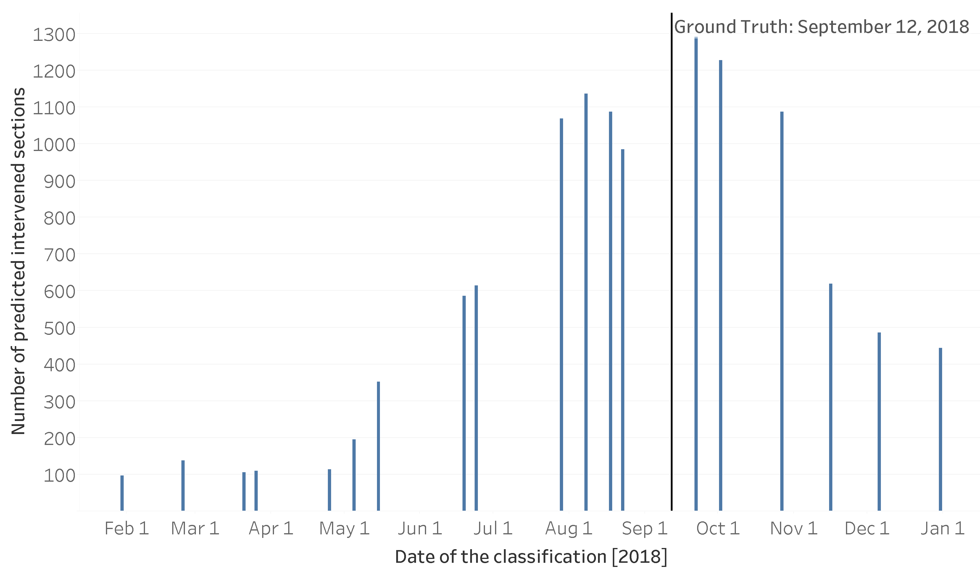
Although the best model performs quite well, the previous results are only shown to one date, 12 September, given there is only ground truth for that particular date. Since the static analysis only uses reference satellite images from one date to train the model, the other left out products can be used to check if the behavior of the algorithm is as expected. This model (RF) was trained with a reference image from 12 September and the ground truth until the same date. The model was then applied for each date that had Sentinel-2 data. This shows how the model behaves with data before (start of the year), during (middle of the year), and after the interventions (end of the year). This analysis is especially interesting because the ground truth shows interventions in FMZs up to 12 September, meaning interventions can appear in images at distinct points in time before that date. In Figure 10 the number of sections classified as treated for each date is presented.

There are no precise metrics for the results of the dates before and during the observed intervention period because the ground truth does not have the date of intervention for each section. As the classification advances throughout the year, the number of detected interventions starts to climb as soon as the first intervention is made. As more FMZs are cleaned throughout the year the model can detect those interventions. After the ground truth date, the number of detected intervention zones starts declining, mainly due to vegetation regrowth and shadows or dark area pixels in the images at the end of the year.

3.2. Temporal Analysis

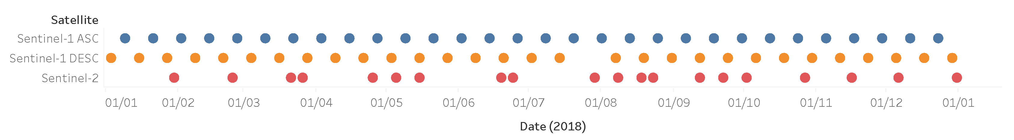
The FMZs along roads were also analyzed using time- series data with three main structures: Sentinel-1 data, Sentinel-2 data, and with the combination of Sentinel-2 and Sentinel-1 data.

3.2.1. One Satellite: Sentinel-1

For the Sentinel-1 data approach, dual-polarization (VV and VH) and multiple orbit (Ascending and Descending) products were used (DS_SAR). Even when using a temporal approach, the precision for this satellite was considerably lower than for Sentinel-2 in the static analysis, fluctuating between an F1-Score of 0.6208 and 0.6872 for all models and with a low Kappa score between 0.2508 and 0.3769. Nevertheless, the RF obtained an F1-score of 0.69. On the other hand, SVM and KNN obtained lower results, since they were unable to classify correctly treated sections, classifying most of the samples as non-treated sections. This behavior is also true for the other models, thus the low Kappa agreement values.

When analyzing in more detail the confusion matrix (

Table 4. Confusion Matrix for the RF algorithm using the Sentinel-1 data (ASC and DESC).

Predicted\Reference	Treated	Not Treated	Total	Precision	Recall	F1-Score
Treated	61	10	71	0.37	0.54	0.44
Not Treated	52	1170	1222	0.96	0.92	0.94
Total	113	1275
Global F1-Score (macro)	0.69
Global Kappa	0.38

) of the RF results, it shows that the metrics of the untreated sections had a great influence on the value of the global F1-score, since the treated sections only had an F1-score 0.44.

3.2.2. One Satellite: Sentinel-2

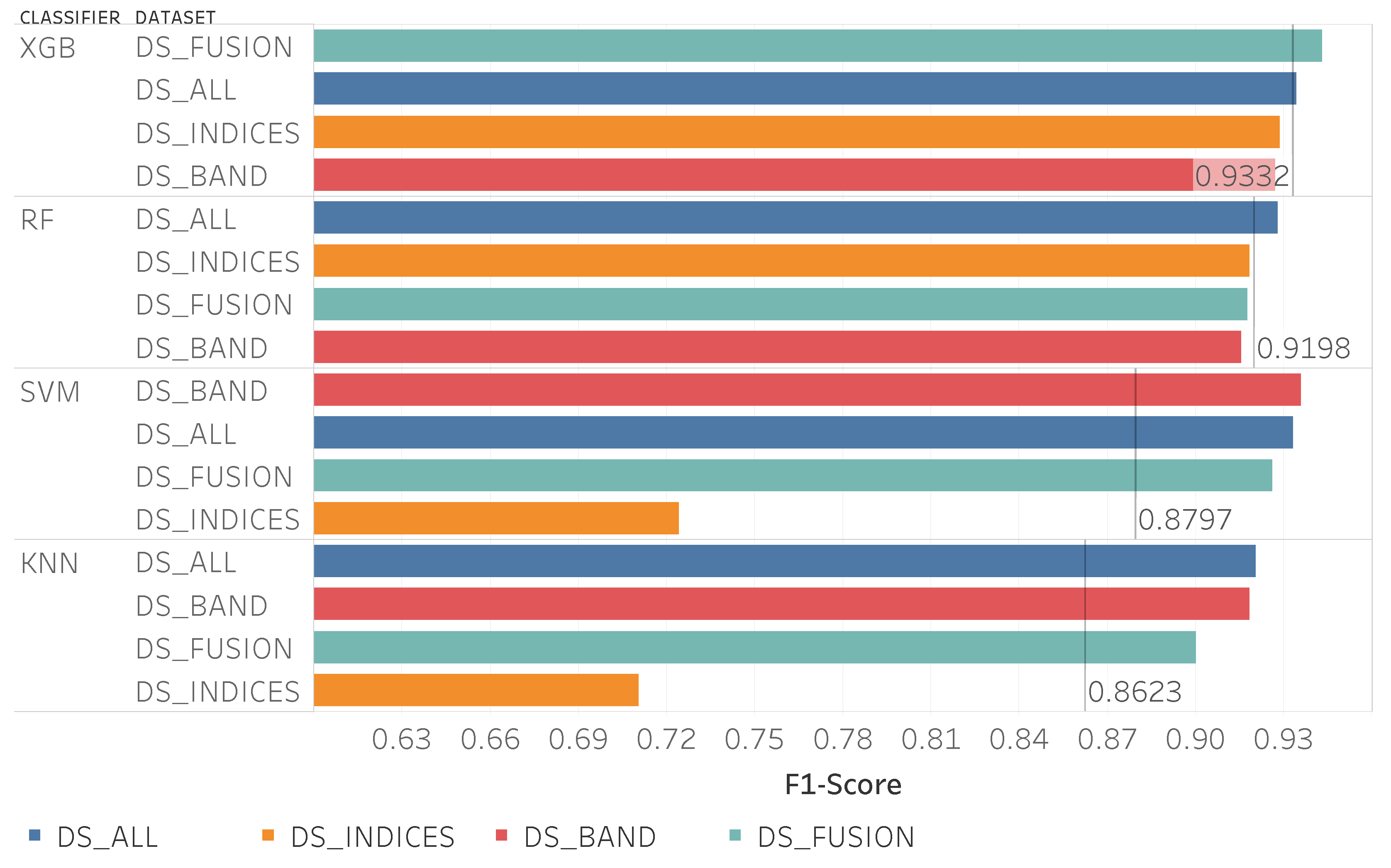
Figure 11 shows the classification results for the time- series experiment using only Sentinel-2 data, note that the data sets are sorted by performance and by model. All data sets, except for DS_INDICES, obtained similar results. Comparing DS_INDICES with the other data sets, for the KNN and SVM algorithms, results were significantly lower, being around 22% lower than the best for the KNN. Unlike the static analysis, the results from the SVM classifier managed to outperform ensemble methods (excluding the data set DS_INDICES). The best algorithm was the SVM with an F1-score of 0.93, nevertheless, XGBoost, and RF generated results that have less variance across data sets.

Table 5. Confusion Matrix for the SVM algorithm using the data set DS_BAND.

Predicted\Reference	Treated	Not Treated	Total	Precision	Recall	F1-Score
Treated	97	10	107	0.91	0.86	0.88
Not Treated	16	1265	1281	0.99	0.99	0.99
Total	113	1275
Global F1-Score (macro)	0.94
Global Kappa	0.87

shows the confusion matrix for the best results, with SVM using the DS_BAND data set. The “not treated” sections class had very high metrics close to 1. For the “treated” sections class, the metrics were lower, but still good, with an F1-score of 0.88, with only 10 sections being incorrectly classified as treated.

Using time-series there is an improvement in the classification of treated and not treated sections for FMZs along roads when compared with the static analysis, with the F1-score of the treated sections class rising from 0.82 to 0.88.

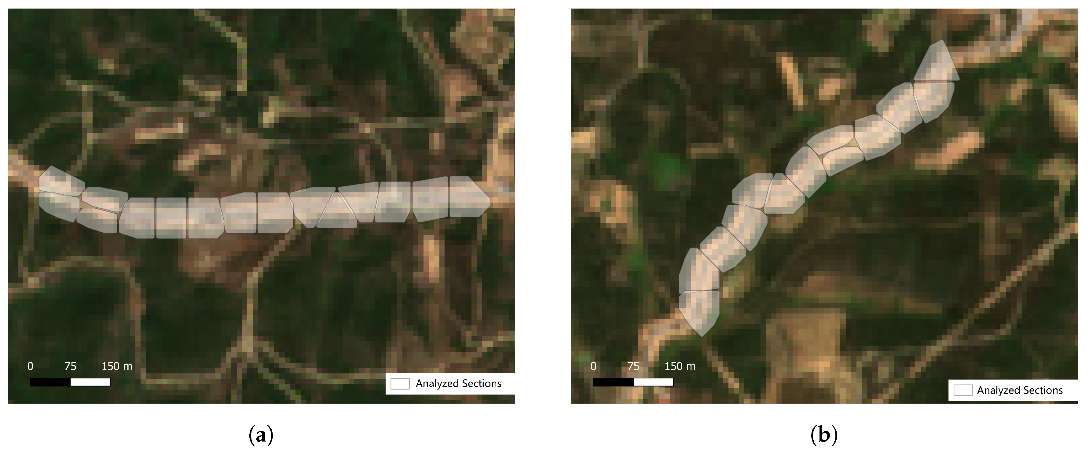
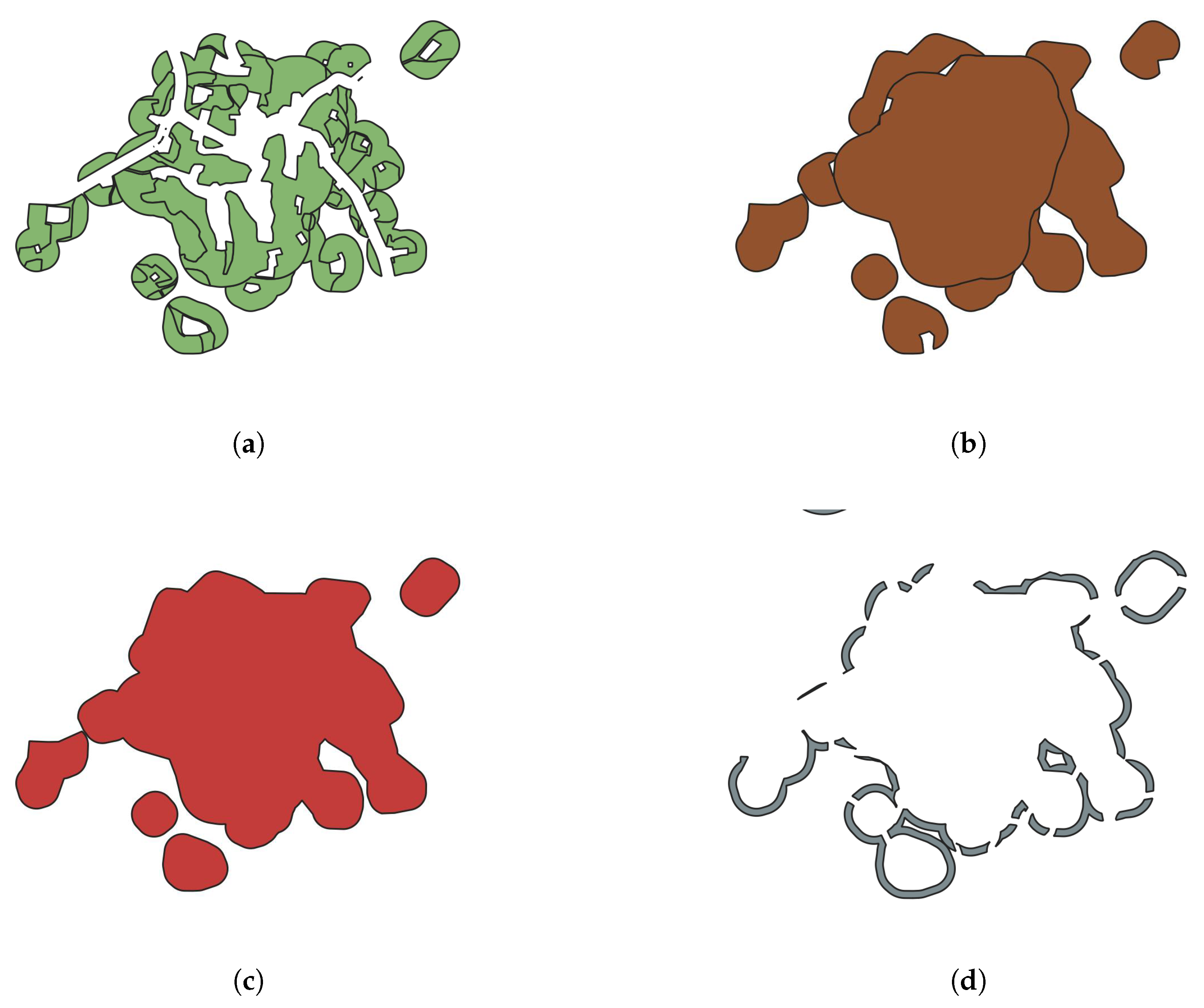
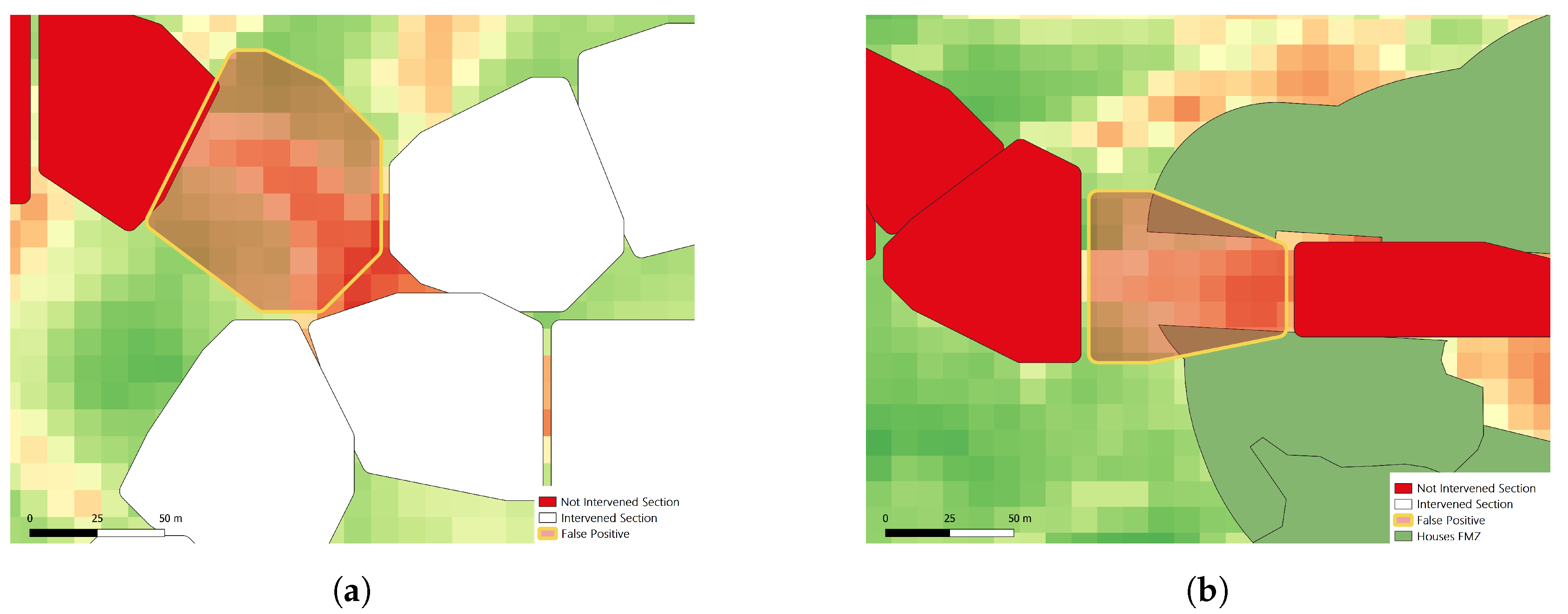
Analyzing the errors in more detail, in Figure 12 there are two examples of sections that were incorrectly classified as treated. These sections are in areas of intersection between FMZs that were treated and FMZs that were not treated (Figure 12a) or in the limit between the interior and exterior of house clusters (Figure 12b).

3.2.3. Both Satellites: Sentinel-1 and Sentinel-2

The information from Sentinel-2 and Sentinel-1 was merged to analyze if it had impact in the results. Figure 13 presents the F1-score values for the different algorithms and data sets, note that the data sets are sorted by performance and by model. Globally these values maintained a behavior similar to the values observed using only Sentinel-2 data. For the SVM, the best F1-score values did not change in comparison to using the Sentinel-2 data. For the RF, the F1-score slightly increased in all data sets. This data combination had the biggest impact in the XGBoost results, raising the F1-score more than 1% in comparison to using just Sentinel-2 data. In this experiment, the XGBoost was the algorithm with the best results reaching an F1-score of 0.94. Overall, using Sentinel-1 data together with Sentinel-2 data showed some improvements in the results of the algorithms.

3.3. Estimation of FMZs Intervention Date

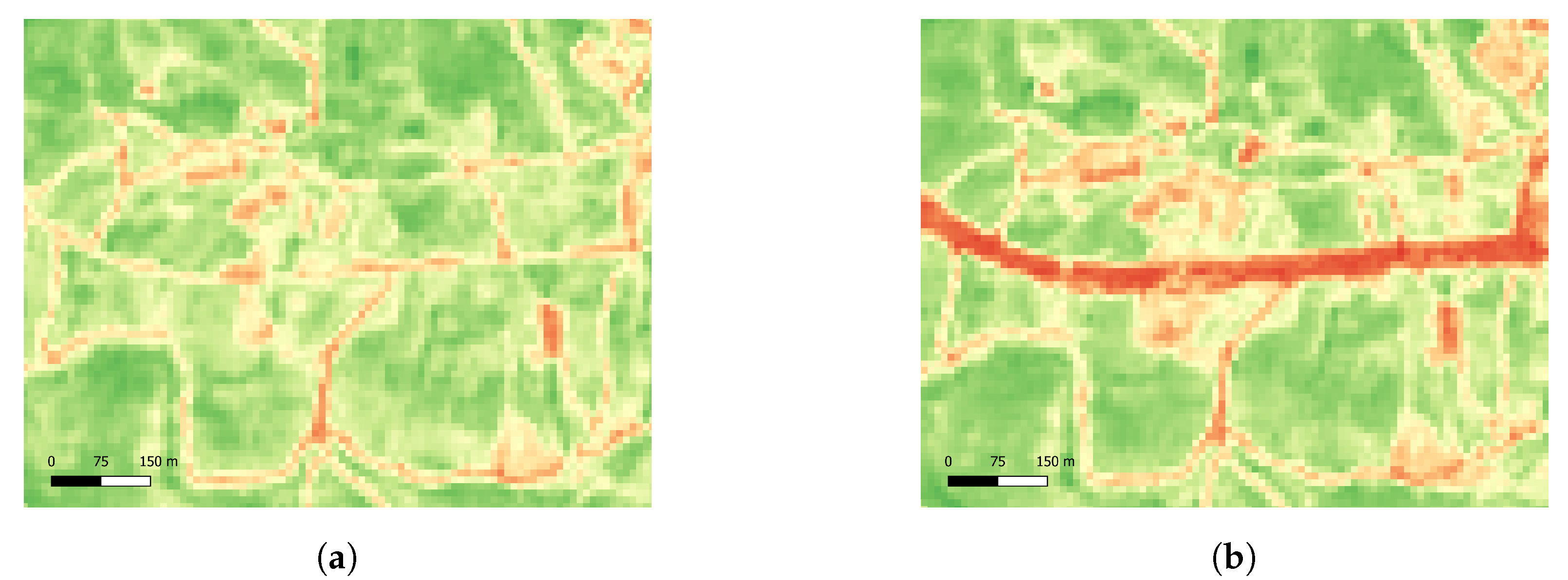
This work aims to classify if FMZs are treated and maintained but it is also interesting to establish when those same FMZs are treated. For this purpose, an extra experiment was carried out to try to estimate the dates on which interventions in FMZs occurred. To achieve this, some clusters sections were selected for further analysis. These sections were treated at the same time of the year, but are part of two different locations: Site A (Figure 14a) and Site B (Figure 14b).

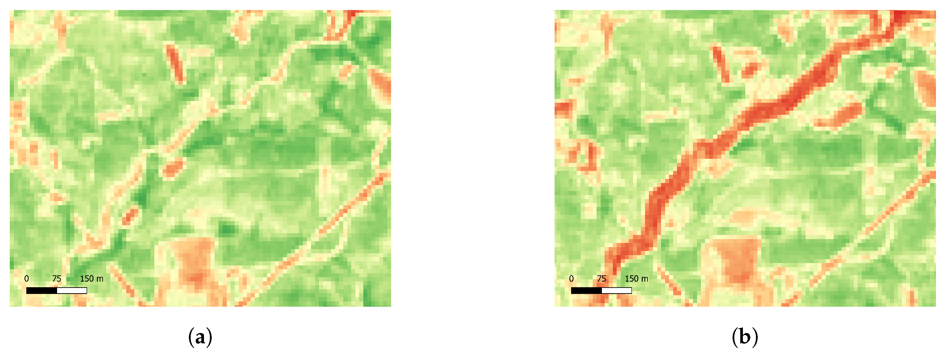
These FMZs in particular were selected due to their official data not being yet available by the Mação City Hall, and because the intervention of FMZs around roads is more easily noticeable in satellite images. As it can be seen in Figure 15, for Site A, the NDVI values before and after intervention have drastic changes. The same can be observed for Site B in Figure 16. A simple threshold value was used as the classifier using the temporal pattern $\mathsf{\Delta }di{f}_{NDVI}$ (Equation (4)) which calculates the difference of the $di{f}_{NDVI}$ (Equation (2)) in two consecutive dates. By establishing a threshold of $l=0.10$, an FMZ is assumed to be treated when $\mathsf{\Delta }di{f}_{NDVI}>l$. This index represents a sudden drop of the FMZ NDVI values in consecutive months, while the values on the outer buffer have little variation.

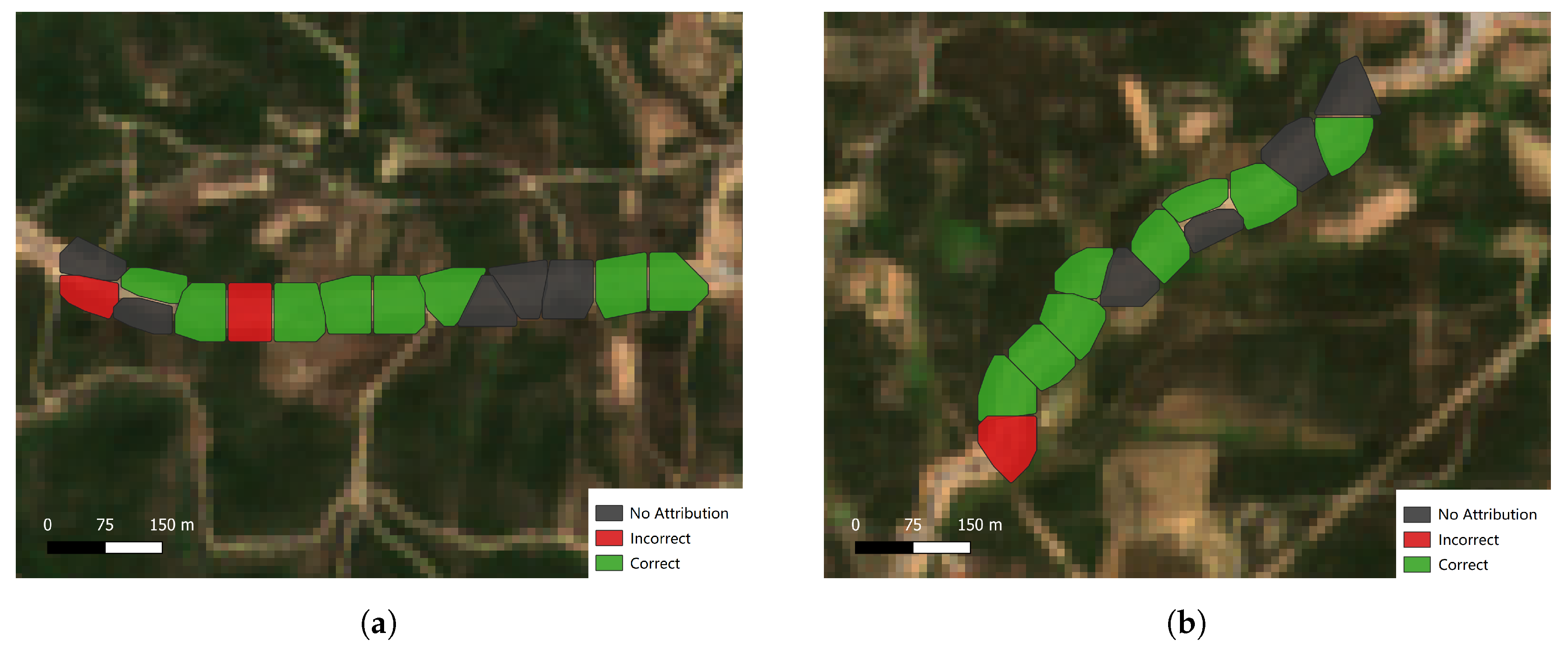
The results for both sites are presented in Figure 17. In both cases, most of the estimated intervention dates correspond to the manual observed date, only failing in 3 cluster sections out of 28. However, for several sections, there were no results. In sum, 16 sections were estimated correctly, 3 incorrectly and 9 had no attribution of an estimated intervention date (i.e., $di{f}_{NDVI}=<0.10$).

4. Discussion

In this paper, two types of analysis were carried out: a static analysis, using only Sentinel-2 data from one date, and a temporal analysis using the temporal patterns of the Sentinel-2 and Sentinel-1 characteristics. The FMZs along roads were analyzed using classification algorithms and temporal patterns to classify which FMZ sections that were treated. An evaluation of the different classification algorithms was also carried out, both in the temporal analysis and in the static analysis, comparing the results of these algorithms using different data sets. In addition to these classification experiments, an experiment was also carried out to try to determine the dates of the intervention of the FMZs along roads. In this section, the results of the various experiments are discussed.

Different classification algorithms were used in this work: RF, SVM, XGBoost, and KNN. The algorithms that stand out are XGBoost and RF, which in almost all experiments achieved the best results. The algorithms that generally obtained the worst results were SVM and KNN. In the static analysis, SVM obtained the lowest results using the data set DS_INDICES. However, in the temporal analysis, the results of these algorithms improved considerably in such a way that SVM was immediately behind XGBoost using data from Sentinel-2. Nevertheless, ensemble methods, such as RF and XGBoost, methods can consistently achieve high performance and the performance per dataset does not vary by a big margin.

Regarding the data, five different data sets were compared: DS_ALL, DS_INDICES, DS_BAND, DS_FUSION, and DS_SAR. In the static analysis, only data from Sentinel-2 was used and in the temporal analysis information from Sentinel-1 was added. In both temporal and static analysis, the DS_ALL data set was always among the data sets with the highest metrics, being the best in most experiments due to having more information available for the algorithms. The DS_INDICES obtained worse results in almost all experiments in comparison to the DS_BAND data set, often with a big difference between the results of both. In the temporal analysis, for the RF and XGBoost algorithms, the DS_INDICES obtained an F1-score close to the best results; however for the SVM and KNN the results were lower, with a difference of 22% for the best result in one of the tests (using KNN in the FMZs along roads). It can be concluded that vegetation indices by themselves are not expressive enough to model the properties of the FMZs to determine if they were treated or not. Furthermore, the SVM and KNN showed a tendency to overfit on DS_INDICES.

The temporal analysis using the data set DS_SAR (just Sentinel-1 data) generated significantly lower results. Although it achieved an average F1-Score, the Kappa reached as low as 0.25. This shows that this type of data is not reliable enough to be used for this type of application. Further research is needed to see if it is possible to leverage more performance from SAR data, either with new models or a different processing pipeline (e.g., adding textural information). SAR data is especially interesting when there is not multispectral data available, for example when there is cloud coverage over the study area. Even with the low performance of SAR, the combination of Sentinel-1 and Sentinel-2 showed slight improvements in the results, with the most significant improvement in the F1-score, increasing by almost 2%. Although the global F1-score is equal when using only Sentinel-2 data and Sentinel-2 in conjunction with Sentinel-1 data, there was a difference in the results for the treated sections class. With just data from Sentinel-2, the treated sections class had an F1-score of 0.88, when adding Sentinel-1 data this value raised to 0.90. The combination of Sentinel-1 and Sentinel-2 can increase the performance of the proposed algorithms. Even though the increase in performance was measured at 2%, the high availability of Sentinel-1 data (not affected by cloud coverage) can be beneficial. However, it must be considered its only main drawback associated with the data prepossessing complexity.

Finally, as it isas it is not only important to know if FMZs are treated but also when, a final experiment was carried out. The main goal was to create an algorithm that could roughly estimate the dates of the interventions. In both study areas, the algorithm performed very well, identifying most of the intervention dates right compared to the ones obtained after a manual examination. This experiment had the role of proof of concept, as the sample size was smaller, but it serves as a starting point for future research on intervention date estimation. This work can aid in solving ambiguities and uncertainty in the ground truth about FMZs.

The thorough research for related work yielded no previous studies that directly approach the analysis of the state of FMZs. In general, the presented results are quite good and showed that the use of remote sensing techniques in conjunction with classification algorithms can help in the detection of interventions in the FMZs, promoting fire protection around the detected areas.

5. Conclusions

This work presented a new method to detect interventions in FMZs using machine- learning algorithms and satellite images from Sentinel-2 and Sentinel-1. Combining machine- learning and open satellite data could reduce the costs associated with manual checkups of FMZs. This process is also scalable as it would only require the extraction of more satellite images over the study area. The main technique used to detect an intervention was to extract information about the vegetation in both the interior and exterior of an FMZ to detect variations. This approach required the creation of buffers outside the FMZ, in vegetation zones, which depending on the type of FMZ can be complex to generate. This information about the interior and exterior of FMZs is then used to generate new features from the input satellite spectral and radiometric images. The proposed method can serve as a baseline for future work into the detection of vegetation growth and maintenance in forest fire-sensitive areas, in this case, the FMZs.

The results show that the usage of satellite data can be used to detect if an FMZ is properly clean and maintained, thus improving forest fire protection. As expected, due to having more information, time-series data had better results than using only a single date. Furthermore, from all the data sets tested, DS_ALL had the best scores overall. Regarding the used machine- learning algorithms, ensemble methods (RF and XGBoost) prove to be robust when working with remote sensing data by having good scores across the board. In the experiments, the best scores were achieved by XGBoost when combined with the best data set, DS_FUSION, which uses spectral and radar data as well as some derived vegetation indices.

Although the results presented in this work refer to road FMZs, other experiments in other types of FMZs were done, in particular for the electrical lines FMZs. Due to some uncertainty about the ground truth of this type of FMZ, the results are not shown here. Nevertheless, the preliminary work is promising, even though it cannot have the same level of certainty of results due to uncertainty in the ground truth. Apart from that, scores for the electrical lines FMZs could be affected by various factors like like regular maintenance due to the risk of fire ignition associated with these lines, making the detection of vegetation change more difficult; the size of the sections for this type of FMZ is smaller resulting in less information in comparison to the road’s sections. Future work will be done to mitigate the uncertainty about the ground truth of these FMZs types, allowing the proposed algorithms to be valuable for many different types of FMZs.

References

1. Instituto da Conservação da Natureza e das Florestas. 8° Relatório Provisório de Incêndios Rurais. Informação Estatística Sobre Incêndios Rurais 1 de Janeiro a 15 de Outubro de 2019; This Document Is Presented in Portuguese; Instituto da Conservação da Natureza e das Florestas: Lisbon, Portugal, 2019.
2. Ministry of Agriculture for Rural Development and Fishing. Decreto-Lei n.° 124/2006. In Diário da República n.° 123/2006, Série I-A de 2006-06-28; (Note: This Document Is Presented in Portuguese); Ministry of Agriculture for Rural Development and Fishing: Ana Paula, Portugal, 2006. [Google Scholar]
3. Administração Interna. Decreto-Lei n.° 10/2018. In Diário da República n.° 32/2018, Série I de 2018-02-14; (Note: This Document Is Presented in Portuguese); Administração Interna: Lisboa Portugal, 2018. [Google Scholar]
4. Instituto da Conservação da Natureza e das Florestas-ICNF. Manual de Rede Primária; Divisão de Proteção Florestal E Valorização de Áreas Públicas (DPFVAP) (Note: This Document Is Presented in Portuguese); Instituto da Conservação da Natureza e das Florestas-ICNF: Lisbon, Portugal, 2014.
5. Noi, P.T.; Kappas, M. Comparison of random forest, k-nearest neighbor, and support vector machine classifiers for land cover classification using sentinel-2 imagery. Sensors 2018, 18, 18. [Google Scholar] [CrossRef] [Green Version]
6. Jiang, H.; Li, D.; Jing, W.; Xu, J.; Huang, J.; Yang, J.; Chen, S. Early Season Mapping of Sugarcane by Applying Machine Learning Algorithms to Sentinel-1A/2 Time Series Data: A Case Study in Zhanjiang City, China. Remote Sens. 2019, 11, 861. [Google Scholar] [CrossRef] [Green Version]
7. Qian, Y.; Zhou, W.; Yan, J.; Li, W.; Han, L. Comparing machine learning classifiers for object-based land cover classification using very high resolution imagery. Remote Sens. 2015, 7, 153–168. [Google Scholar] [CrossRef]
8. Immitzer, M.; Vuolo, F.; Atzberger, C. First experience with Sentinel-2 data for crop and tree species classifications in central Europe. Remote Sens. 2016, 8, 166. [Google Scholar] [CrossRef]
9. Maltsev, E.; Maglinets, Y.; Tsibulskii, G. The Technology to Identify Firebreak Plowing Objects Based on the Satellite Data of the Earth Remote Sensing. E3S Web Conf. 2019, 75, 01006. [Google Scholar] [CrossRef]
10. Liampas, S.-A.G.; Stamatiou, C.C.; Drosos, V.C. Comparison of three DEM sources: A case study from Greek forests. In Proceedings of the Sixth International Conference on Remote Sensing and Geoinformation of Environment, Paphos, Cyprus, 26–29 March 2018; Volume 10773. [Google Scholar] [CrossRef]
11. Belgiu, M.; Csillik, O. Sentinel-2 cropland mapping using pixel-based and object-based time-weighted dynamic time warping analysis. Remote Sens. Environ. 2018, 204, 509–523. [Google Scholar] [CrossRef]
12. Peña, M.A.; Liao, R.; Brenning, A. Using spectrotemporal indices to improve the fruit-tree crop classification accuracy. ISPRS J. Photogramm. Remote Sens. 2017, 128, 158–169. [Google Scholar] [CrossRef]
13. Erinjery, J.J.; Singh, M.; Kent, R. Mapping and assessment of vegetation types in the tropical rainforests of the Western Ghats using multispectral Sentinel-2 and SAR Sentinel-1 satellite imagery. Remote Sens. Environ. 2018, 216, 345–354. [Google Scholar] [CrossRef]
14. Müller, H.; Rufin, P.; Griffiths, P.; Barros Siqueira, A.J.; Hostert, P. Mining dense Landsat time series for separating cropland and pasture in a heterogeneous Brazilian savanna landscape. Remote Sens. Environ. 2015, 156, 490–499. [Google Scholar] [CrossRef] [Green Version]
15. Pelletier, C.; Valero, S.; Inglada, J.; Champion, N.; Dedieu, G. Assessing the robustness of Random Forests to map land cover with high resolution satellite image time series over large areas. Remote Sens. Environ. 2016, 187, 156–168. [Google Scholar] [CrossRef]
16. Gómez, C.; White, J.C.; Wulder, M.A. Optical remotely sensed time series data for land cover classification: A review. ISPRS J. Photogramm. Remote Sens. 2016. [Google Scholar] [CrossRef] [Green Version]
17. Clevers, J.G.; Kooistra, L.; van den Brande, M.M. Using Sentinel-2 data for retrieving LAI and leaf and canopy chlorophyll content of a potato crop. Remote Sens. 2017, 9, 405. [Google Scholar] [CrossRef] [Green Version]
18. Piragnolo, M.; Lusiani, G.; Pirotti, F. Comparison of vegetation indices from RPAS and Sentinel-2 imagery for detecting permanent pastures. Int. Arch. Photogramm. Remote Sens. Spat. Inf. Sci. ISPRS Arch. 2018, 42, 1381–1387. [Google Scholar] [CrossRef] [Green Version]
19. Rozenstein, O.; Haymann, N.; Kaplan, G.; Tanny, J. Estimating cotton water consumption using a time series of Sentinel-2 imagery. Agric. Water Manag. 2018, 207, 44–52. [Google Scholar] [CrossRef]
20. Satir, O.; Berberoglu, S. Crop yield prediction under soil salinity using satellite derived vegetation indices. Field Crops Res. 2016, 192, 134–143. [Google Scholar] [CrossRef]
21. Setiyono, T.D.; Quicho, E.D.; Gatti, L.; CamposTaberner, M.; Busetto, L.; Collivignarelli, F.; GarciaHaro, F.J.; Boschetti, M.; Khan, N.I.; Holecz, F. Spatial rice yield estimation based on MODIS and Sentinel-1 SAR data and ORYZA crop growth model. Remote Sens. 2018, 10, 293. [Google Scholar] [CrossRef] [Green Version]
22. Castillo, J.A.A.; Apan, A.A.; Maraseni, T.N.; Salmo, S.G. Estimation and mapping of above-ground biomass of mangrove forests and their replacement land uses in the Philippines using Sentinel imagery. ISPRS J. Photogramm. Remote Sens. 2017, 134, 70–85. [Google Scholar] [CrossRef]
23. Jiang, Z.; Huete, A.; Chen, J.; Chen, Y.; Li, J.; Yan, G.; Zou, Y. Analysis of NDVI and scaled difference vegetation index retrievals of vegetation fraction. Remote Sens. Environ. 2006, 101, 366–378. [Google Scholar] [CrossRef]
24. Huete, A. A soil-adjusted vegetation index (SAVI). Remote Sens. Environ. 1988, 25, 295–309. [Google Scholar] [CrossRef]
25. Jordan, C. Derivation of Leaf-Area Index from Quality of Light on the Forest Floor. Ecology 1969, 50. [Google Scholar] [CrossRef]
26. Frampton, W.J.; Dash, J.; Watmough, G.; Milton, E.J. Evaluating the capabilities of Sentinel-2 for quantitative estimation of biophysical variables in vegetation. ISPRS J. Photogramm. Remote Sens. 2013, 82, 83–92. [Google Scholar] [CrossRef] [Green Version]
27. Gao, B.C. NDWI-A normalized difference water index for remote sensing of vegetation liquid water from space. Remote Sens. Environ. 1996, 58, 257–266. [Google Scholar] [CrossRef]
28. Hadjimitsis, D.G.; Papadavid, G.; Agapiou, A.; Themistocleous, K.; Hadjimitsis, M.G.; Retalis, A.; Michaelides, S.; Chrysoulakis, N.; Toulios, L.; Clayton, C.R.I. Atmospheric correction for satellite remotely sensed data intended for agricultural applications: Impact on vegetation indices. Nat. Hazards Earth Syst. Sci. 2010, 10, 89–95. [Google Scholar] [CrossRef] [Green Version]
29. Agapiou, A.; Hadjimitsis, D.G.; Papoutsa, C.; Alexakis, D.D.; Papadavid, G. The Importance of accounting for atmospheric effects in the application of NDVI and interpretation of satellite imagery supporting archaeological research: The case studies of Palaepaphos and Nea Paphos sites in Cyprus. Remote Sens. 2011, 3, 2605–2629. [Google Scholar] [CrossRef] [Green Version]
30. Main-Knorn, M.; Pflug, B.; Louis, J.; Debaecker, V.; Müller-Wilm, U.; Gascon, F. Sen2Cor for Sentinel-2. In Image and Signal Processing for Remote Sensing XXIII; Bruzzone, L., Ed.; International Society for Optics and Photonics SPIE: Bellingham, WA, USA, 2017; Volume 10427, pp. 37–48. [Google Scholar] [CrossRef] [Green Version]
31. Moreira, A.; Santos, M.Y. Concave hull: A k-nearest neighbours approach for the computation of the region occupied by a set of points. In Proceedings of the GRAPP 2007, Second International Conference on Computer Graphics Theory and Applications, Barcelona, Spain, 8–11 March 2007. [Google Scholar]
32. OpenStreetMap Contributors. 2019. Planet Dump Retrieved from https://planet.osm.org. Available online: https://www.openstreetmap.org (accessed on 26 March 2019).
33. MacQueen, J. Some methods for classification and analysis of multivariate observations. In Proceedings of the Fifth Berkeley Symposium on Mathematical Statistics and Probability, Berkeley, CA, USA, 21 June–18 July 1965; Volume 1, pp. 281–297. [Google Scholar]
34. Abdikan, S.; Sanli, F.B.; Ustuner, M.; Calo, F. Land cover mapping using sentinel-1 sar data. ISPRS Int. Arch. Photogramm. Remote Sens. Spat. Inf. Sci. 2016, XLI-B7, 757–761. [Google Scholar] [CrossRef]
Figure 1. Study area and some Fuel Management Zones (FMZs) in vector format in the zone of Cardigos, Mação. Please note that the images are not in scale.
Ijgi 09 00533 g001
Figure 2. Fuel Management Zones (FMZs) along roads and powerlines, in the north of Mação, which were treated in 2018.
Ijgi 09 00533 g002
Figure 3. Temporal distribution of the images used from both satellites, Sentinel-2 and both orbits from Sentinel-1 throughout 2018.
Ijgi 09 00533 g003
Figure 4. Vector information of Fuel Management Zones (FMZs) in the north of Mação.
Ijgi 09 00533 g004
Figure 5. Example of the phases to create the outer buffers. (a) Polygon that represents a Fuel Management Zones (FMZ) along electrical lines, with a width of 15 m. (b) Polygon resulting from using the 20 m Buffer function. (c) Polygons that represent only external areas of the FMZ, after removing the middle of the FMZ and roads from OpenStreetMaps.
Ijgi 09 00533 g005
Figure 6. Example of the processing chain to obtain the interior of the Fuel Management Zones (FMZs) around housing. (a) Initial FMZ; (b) Concave Hull applied; (c) Polygon dissolveddissolved, and holes removed; (d) Difference between the FMZ with a 20 m buffer and the polygon that represents the interior of the initial FMZ, after removing roads from OpenStreetMaps.
Ijgi 09 00533 g006
Figure 7. Stages of segment creation. (a) Points of the interior (orange) and the exterior buffer of the FMZ (gray). (b) Clusters generated using K-Means. K = 5200.
Ijgi 09 00533 g007
Figure 8. Examples of the intersection of Fuel Management Zones (FMZs) and buffers with the created sections. (a) Section of an FMZ along a road. (b) Section of an FMZ along an electric line. (c) Section of an FMZ around a cluster of dwellings.
Ijgi 09 00533 g008
Figure 9. F1-score values of the different algorithms and data sets, for the Fuel Management Zones (FMZs) along roads.
Ijgi 09 00533 g009
Figure 10. Number of sections classified as treated using the best model (RF with DS_ALL) along the whole year of 2018. Trained with data of 12 of September.
Ijgi 09 00533 g010
Figure 11. F1-score value for all algorithms and data sets using just Sentinel-2 data.
Ijgi 09 00533 g011
Figure 12. Examples of false positives obtained using the SVM with the data set DS_BAND.
Ijgi 09 00533 g012
Figure 13. F1-score values for all algorithms and data sets using Sentinel-1 and Sentinel-2 data.
Ijgi 09 00533 g013
Figure 14. Sections used to estimate the intervention date.
Ijgi 09 00533 g014
Figure 15. NDVI before and after the intervention for Site A. (a) NDVI on 15 May 2018. (b) NDVI on 19 June 2018.
Ijgi 09 00533 g015
Figure 16. NDVI before and after the intervention for Site B. (a) NDVI on 15 May 2018. (b) NDVI on 19 June 2018.
Ijgi 09 00533 g016
Figure 17. Intervention date forecast results for Site A (a) and Site B (b). Presented in red where the estimate was wrong, in green where it was correct, and in black which did not obtain results.
Ijgi 09 00533 g017