Comparing Machine and Deep Learning Methods for Large 3D Heritage Semantic Segmentation

Abstract

In recent years semantic segmentation of 3D point clouds has been an argument that involves different fields of application. Cultural heritage scenarios have become the subject of this study mainly thanks to the development of photogrammetry and laser scanning techniques. Classification algorithms based on machine and deep learning methods allow to process huge amounts of data as 3D point clouds. In this context, the aim of this paper is to make a comparison between machine and deep learning methods for large 3D cultural heritage classification. Then, considering the best performances of both techniques, it proposes an architecture named DGCNN-Mod+3Dfeat that combines the positive aspects and advantages of these two methodologies for semantic segmentation of cultural heritage point clouds. To demonstrate the validity of our idea, several experiments from the ArCH benchmark are reported and commented.

1. Introduction

Semantic segmentation is one of the most important research methods for computer vision, and has the task to classify each pixel or point in the scene into classes that have specific features [1,2]. In the past, semantic segmentation concerned bi-dimensional images but, due to some limitations related to occlusions, illumination, posture and other problems, the researches began to deal with three-dimensional data. This change also occurred thanks to the growing diffusion of photogrammetry and laser scanning surveys. In the 3D form of semantic segmentation, regular or irregular points are processed in the 3D space [3].

Surely, the automatic interpretation of 3D point clouds by semantic segmentation in the cultural heritage (CH) context represents a very challenging task. Digital documentation is not easy to obtain, but it is necessary to disseminate cultural heritage [4]. Shapes are complex and the objects, even if repeatable, are unique, handcrafted and not serialised. Notwithstanding, the understanding of 3D scenes in digital CH is crucial, as it can have many applications such as the identification of similar architectural elements in large dataset, the analysis of the state of conservation of materials, the subdivision of the point clouds in its structural parts preliminary for scan-to-BIM processes, etc. [5].

In recent years, the researches for semantic segmentation of point clouds in CH have made a significant breakthrough thanks to the application of artificial intelligence (AI) methods [6,7]. In the literature, most of the machine learning (ML) and deep learning (DL) approaches employ supervised learning methods. According to [8] in the era of big-data, ML classification approaches are evolving in DL approaches since they are more efficient to deal with a large quantity of data derived from modern methods and with the complexity of 3D point clouds, by continuously teaching and adjusting their abilities [9,10,11]. However, as their success relies on the availability of large amounts of annotated dataset, the complete replacement of ML approaches within the heritage field is still not possible. A major drawback of DL methods is that they are not easily interpretable, since these models behave as black-boxes and fail to provide explanations on their predictions.

In this context, the aim of this research is to report a comparison between two different classification approaches for CH scenarios, based on machine and deep learning techniques. Among them, four state-of-the-art ML and DL algorithms are tested, highlighting the possibility to combine the positive aspects of each methodology into a new architecture (later called DGCNN-Mod+3Dfeat) for the semantic segmentation of CH 3D architectures.

Among ML methods, we used K-Nearest Neighbours (kNN) [12], Naive Bayes (NB) [13], Decision Trees (DT) [14] and Random Forest (RF) [15]. They have been trained with geometric features and small annotated patches, ad-hoc selected over the different case studies.

Regarding the DL approaches, four different versions of DGCNN [16] are used, trained on several scenes of the newly proposed heritage ArCH benchmark [17], composed of various annotated CH point clouds. Two out of the four DGCNN architectures proposed (DGCNN and DGCNN-Mod) have already been tested by the authors in a previous paper [18] where, from a comparison with other state-of-art NNs (PointNet, PointNet++, PCNN, DGCNN) the DGCNN proved to be the best architecture for our data. Therefore, in this paper, the previously presented results are compared with those achieved introducing new features to the networks.

The evaluation of the selected ML and DL methods is performed on three different heritage scenes belonging to the above cited ArCH dataset.

Research Questions and Paper Structure

In the context of CH-related point cloud classification and semantic segmentation methods, four research questions are addressed by this study:

RQ1

Is it possible to provide the research community with guidelines for the automatic segmentation of point clouds in the CH domain?

RQ2

Which ML and DL algorithms perform better for the semantic segmentation of heritage 3D point cloud?

RQ3

Is there a winning solution between ML and DL in the CH domain?

RQ4

Is it correct comparing the performance results of ML and DL algorithms with the same pipeline?

The paper is organised as follows. Section 2 provides a description of the approaches that were adopted for point clouds semantic segmentation. Section 3 describes the used dataset and methodology. Section 4 offers an extensive comparative evaluation and analysis of ML and DL approaches. A detailed discussion of the results is presented in Section 5. Finally, Section 6 draws conclusions and discusses future directions for this field of research.

Additional experiments have been finally run with the DL methods on the whole ArCH dataset (that includes four new CH labelled scenes, if compared with the 12 used for the previous tests presented in [18]), in order to check if the largest size of the training dataset would effectively improve the performances (see Appendix A,

Table A4. Tests performed on the A_SMV scene, with the whole ArCH dataset as training. Fourteen scenes as training, 1 for validation (5_SMV_chapel_1) and 1 for test.

Network	Metrics	Mean	Arch	Col	Mold	Floor	Do-Wi	Wall	Stair	Vault	Roof
DGCNN	Overall Accuracy	0.7516
	Precision	0.7706	0.0945	0.1783	0.2505	0.6248	0.2625	0.7544	0.7396	0.7058	0.9648
	Recall	0.7516	0.0517	0.0892	0.3849	0.7819	0.1619	0.9004	0.1039	0.8973	0.8359
	F1-Score	0.7398	0.0669	0.1189	0.3035	0.6946	0.2003	0.8210	0.1823	0.7901	0.8958
	IoU	0.3534	0.0345	0.0631	0.1788	0.5320	0.1112	0.6963	0.1002	0.6530	0.8111
DGCNN- Mod	Overall Accuracy	0.8368
	Precision	0.8285	0.2891	0.7626	0.4143	0.8251	0.7785	0.7870	0.8007	0.7922	0.9496
	Recall	0.8369	0.0804	0.1916	0.3598	0.8739	0.1778	0.9266	0.4979	0.9511	0.9361
	F1-Score	0.8223	0.1258	0.3062	0.3851	0.8488	0.2894	0.8511	0.6164	0.8644	0.9428
	IoU	0.4699	0.0671	0.1807	0.2384	0.7372	0.1692	0.7407	0.4429	0.7612	0.8918
DGCNN- 3Dfeat	Overall Accuracy	0.8282
	Precision	0.8253	0.3499	0.6953	0.4139	0.7220	0.3576	0.8428	0.9290	0.6936	0.9572
	Recall	0.8283	0.2824	0.7732	0.3242	0.7103	0.1375	0.8829	0.7095	0.9170	0.9306
	F1-Score	0.8226	0.3126	0.7322	0.3636	0.7161	0.1987	0.8624	0.8045	0.7898	0.9437
	IoU	0.5144	0.1852	0.5775	0.2221	0.5578	0.1102	0.7580	0.6729	0.6525	0.8934
DGCNN- Mod+3Dfeat	Overall Accuracy	0.8645
	Precision	0.8532	0.2619	0.6940	0.5217	0.7927	0.5660	0.8447	0.8563	0.8295	0.9611
	Recall	0.8646	0.0631	0.6780	0.4418	0.8921	0.2615	0.8999	0.7837	0.9474	0.9464
	F1-Score	0.8557	0.1017	0.6859	0.4784	0.8394	0.3578	0.8714	0.8184	0.8845	0.9537
	IoU	0.5555	0.0535	0.5219	0.3144	0.7233	0.2178	0.7721	0.6926	0.7929	0.9114

and

Table A5. Tests performed on the B_SMG scene, with the whole ArCH dataset as training. Fourteen scenes as training, 1 for validation (5_SMV_chapel_1) and 1 for test.

Network	Metrics	Mean	Arch	Col	Mold	Floor	Do-Wi	Wall	Stair	Vault	Roof
DGCNN	Overall Accuracy	0.7836
	Precision	0.8221	0.0008	0.8858	0.1731	0.8827	0.1862	0.7292	0.3888	0.6246	0.9592
	Recall	0.7837	0.0021	0.2405	0.2260	0.6684	0.1362	0.9125	0.5093	0.8327	0.8560
	F1-Score	0.7939	0.0012	0.3783	0.1961	0.7608	0.1573	0.8106	0.4410	0.7138	0.9046
	IoU	0.3763	0.0006	0.2332	0.1086	0.6139	0.0853	0.6815	0.2828	0.5549	0.8259
DGCNN- Mod	Overall Accuracy	0.8958
	Precision	0.8926	0.4766	0.8115	0.4809	0.9653	0.1336	0.8338	0.3568	0.9046	0.9545
	Recall	0.8958	0.2325	0.7875	0.3175	0.8539	0.1415	0.8992	0.4853	0.9446	0.9876
	F1-Score	0.8920	0.3126	0.7993	0.3825	0.9062	0.1374	0.8653	0.4112	0.9242	0.9708
	IoU	0.5348	0.1852	0.6657	0.2364	0.8284	0.0737	0.7625	0.2588	0.8590	0.9432
DGCNN- 3Dfeat	Overall Accuracy	0.8318
	Precision	0.8158	0.3956	0.7101	0.3715	0.8150	0.3312	0.8125	0.8818	0.7074	0.9409
	Recall	0.8319	0.1195	0.6900	0.1893	0.7180	0.2046	0.8705	0.8094	0.9361	0.9495
	F1-Score	0.8181	0.1836	0.6999	0.2508	0.7634	0.2529	0.8405	0.8440	0.8058	0.9452
	IoU	0.5078	0.1010	0.5383	0.1433	0.6173	0.1447	0.7249	0.7301	0.6747	0.8960
DGCNN- Mod+3Dfeat	Overall Accuracy	0.9144
	Precision	0.9173	0.5318	0.8497	0.6502	0.9566	0.1355	0.8797	0.4661	0.8909	0.9753
	Recall	0.9145	0.2578	0.9250	0.5959	0.9030	0.1956	0.8551	0.7101	0.9688	0.9880
	F1-Score	0.9148	0.3472	0.8858	0.6219	0.9290	0.1601	0.8672	0.5628	0.9282	0.9816
	IoU	0.5997	0.2100	0.7949	0.4512	0.8673	0.0870	0.7655	0.3915	0.8660	0.9630

for detailed metrics). The results shown in the paper do not include these four new scenes because it would have compromised a fair comparison with the DGCNN-Mod presented in [18], therefore the same number of scenes has been kept.

2. Related Works

In the literature, there is a restricted number of applications that use machine learning methods to classify 3D point clouds in different objects belonging to cultural heritage scenes, even if, according to [6], these methods had great progress to this regard. Indeed, in their study the authors explore the applicability of supervised machine learning approaches to cultural heritage by providing a standardised pipeline for several case studies.

In this domain, the research of [19] has two main objectives: providing a framework that extracts geometric primitives from a masonry image, and extracting and selecting statistical features for the automatic clustering of masonry. The authors combine existing image processing and machine learning tools for the image-based classification of masonry walls and then make a performances comparison among five different machine learning algorithms for the classification task. The main issue of this method is that each block of the wall is not individually characterised.

The research presented in [20] wants to overcome this limitation, presenting a novel automatic segmentation algorithm of masonry blocks from a 3D point cloud acquired with LiDAR technology. The image processing algorithm is based on an optimisation of the watershed algorithm, also used to improve segmentation algorithms in other works [21,22], to automatically segment 3D point clouds in 3D space isolating each single stone block.

In their research, Grilli et al. [23] propose a strategy to classify heritage 3D models by applying supervised machine learning classification algorithms to their UV maps. To verify the reliability of the method, the authors evaluate different classifiers over three heterogeneous case studies.

In [24] the authors explore the relation between covariance features and architectural elements using supervised machine learning classifier (Random Forest), finding in particular a correlation between the feature search radii and the size of the element. A more in-depth analysis of the previous approach [25] demonstrates the capability of the algorithm to generalise across different unseen architectural scenarios. The research conducted by Murtiyoso et al. [26] aims to help the manual point clouds labeling of large training data set required from machine learning algorithms. Moreover, the authors introduce a series of functions that allow the automatic processing for some issues of segmentation and classification of CH point clouds. Due to the complexity of the problem, the project considers only some important classes. The toolbox uses a multi-scale approach: the point clouds are processed from the historical complex to architectural elements, making it suitable for different types of heritage.

Mainly in recent years, deep learning has received increasing attention from the researches and has been successfully applied to semantically segment 3D point clouds in different domains [3,27]. In the context of cultural heritage there are still few studies that use deep learning approaches to classify 3D point clouds. The need to have a large scale well-annotated dataset can limit its development, blocking the research in this direction. In some cases this problem can be solved using synthetic dataset [8,28]. However, the researches conducted so far have yielded encouraging results.

Deep learning approaches are properly used for directly managing the raw data of point clouds without considering an intermediate processing that allows a more regular representation. For this purpose the first approach is proposed in [29]. An extended version of the previous network considers not only each point separately, but also its neighbors, in order to exploit the local features and thus obtain more efficient classification results [30].

Malinverni et al. [7] use PointNet++ to semantically segment 3D point clouds of CH dataset. The aim of the paper is to demonstrate the efficiency of chosen deep learning approaches to process point clouds of CH domain. Moreover, the method is evaluated on a suitably created CH dataset manually annotated by domain experts.

An alternative to these approaches is based on the point clouds Convolutional Neural Network (PCNN) [31], a novel architecture that uses two operators (extension and restriction). The extension maps functions defined over the point cloud to volumetric functions, while the restriction operator does the inverse.

An approach inspired by PointNet is proposed by [16] where the difference is to exploit local geometric structures using a neural network module, EdgeConv, that constructs a local neighborhood graph and applies convolution-like operations. Moreover the model, named DGCNN (Dynamic Graph Convolutional Neural Network), dynamically updates the graph, changing the set of k-nearest neighbors of a point from layer to layer of the network.

In the CH context, inspired by this architecture, Pierdicca et al. [18] propose to semantically segment 3D point clouds using an augmented DGCNN by adding features such as normals and the radiometric component. This modified version has the aim to simplify the management of DCH assets that have complex geometries, extremely variable and defined with a high level of detail. The authors also propose a novel publicly available dataset to validate the novel architecture making a comparison between other DL methods.

Another study that uses DL to classify objects of CH is presented in [5]. The authors make a performances comparison between machine and deep learning methods in the classification task of two different heritage datasets. Using machine learning approaches (Random Forest and One-versus-One) the performances are excellent in almost all the identified classes, but there is no correlation between the characteristics. Using DL approaches (1D CNN, 2D CNN and RNN Bi-LSTM) the 3D point clouds are considered as a sequence of points. However ML approaches overcome DL, because according to the authors the DL methods implemented are not very recent, and so other architecture will be tested.

3. Materials and Methods

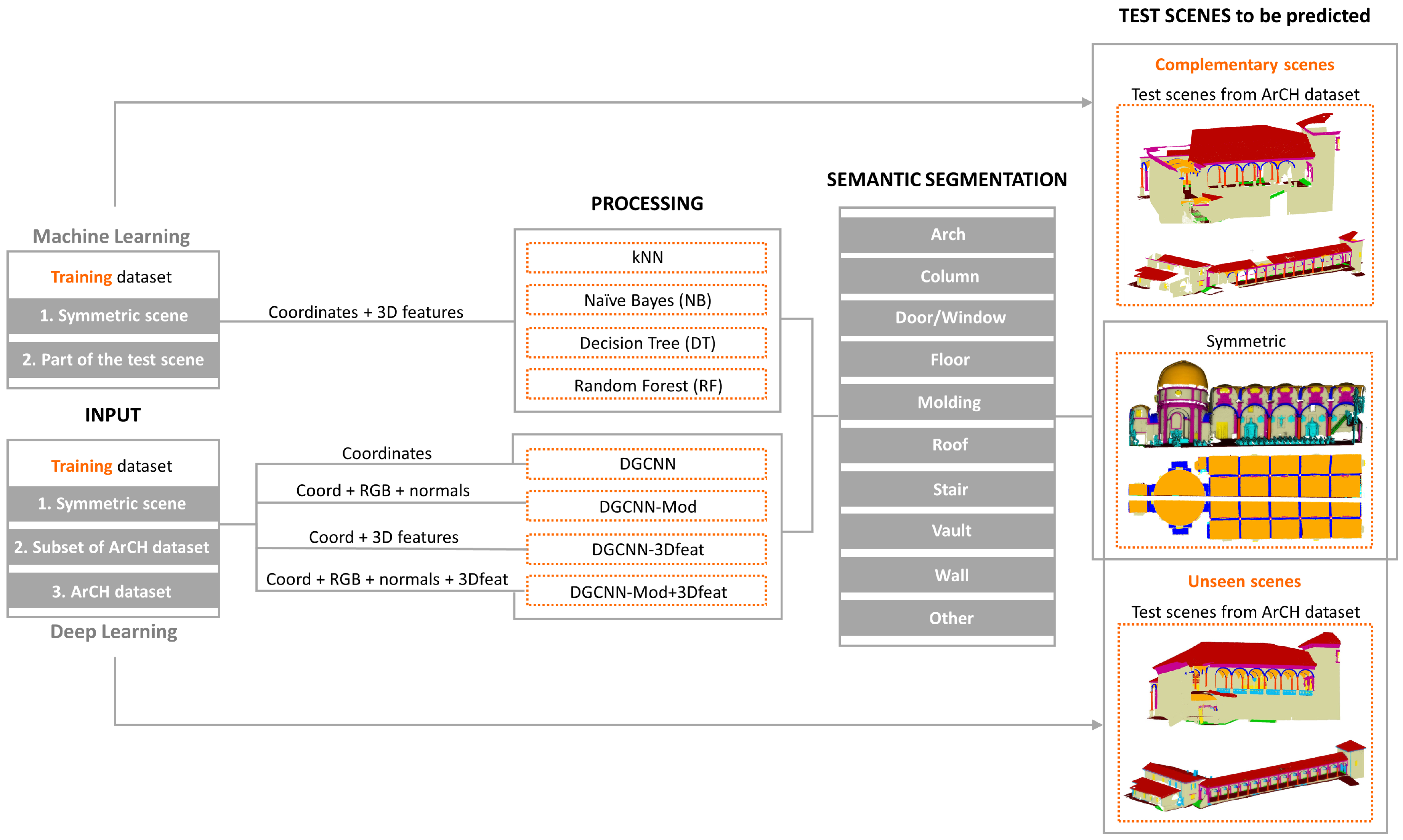
In this section the workflow of the comparison between the two methodologies is presented, as well as the classifiers and scenes used for the three experiments (Figure 1).

As previously mentioned, the goal of this paper is not to compare algorithms, but rather classification approaches. In fact, for a fair comparison between classification algorithms, it would be necessary to use the same training data. In this context, some initial experiments using the same number of scenes in the training phases for both DL and ML algorithms have been performed. However, the ML classifiers did not achieve satisfactory results compared with those obtained using reduced annotated portions of the test scenes. Therefore, as the aim of the paper is discussing the best approaches for heritage classification, a comparison between ML and DL approaches is presented, where the training data are different.

Three different experiments have been performed as follows. In the first experiment both the different ML and DL classifiers have been trained on the same portion of a symmetrical scene: half of the point cloud is used for training and validation, and half for the final test. In the second and third experiment the samples used to train the ML and DL classifiers are different. On one hand, for the ML approach, a reduced portion of the test scene is annotated and used during the training phase, leaving the remaining part for the prediction phase. On the other, for the DL approach, different annotated scenes are used for the training phase, while for the testing totally new data are presented to the networks. Further details are given in the following subsections.

3.1. Benchmark for Point Cloud Semantic Segmentation

The scenes used for the following tests are part of the ArCH benchmark [17], a group of architectural point clouds collected by several universities and research bodies with the aim of sharing and labelling an adequate number of point clouds for training and testing artificial intelligence methods.

This benchmark represents the current state of the art in the field of annotated cultural heritage point clouds, with 15 point clouds of architectural scenarios for training and two for test. Although other benchmarks and datasets for point clouds’ classification and semantic segmentation already exist [32,33,34,35], the ArCH dataset is the only one specifically focused on the CH domain and with a higher level of detail, therefore it has been chosen for the tests here presented.

For our experiments, three test scenes are used (

Table 1. Experiments performed with relative test and training sets.

Experiment	Test Set	Training Set
		ML	DL
1 Overall Results in Table 2 and Figure 4 Detailed Results in Table A1	Trompone Church - symmetrical half part -	Remaining half part	Remaining half part (Training and Validation)	/
2 Overall Results in Table 3 and Figure 6 Detailed Results in Table A2	SMV scene (Sacred Mount of Varallo)	16% of the test scene	10 scenes for Training and 1 for Validation	14 scenes for Training and 1 for Validation (whole ArCH dataset) Results in Table A4
3 Overall Results in Table 4 and Figure 8 Detailed Results in Table A3	SMG scene (Sacred Mount of Ghiffa)	20% of the test scene	10 scenes for Training and 1 for Validation	14 scenes for Training and 1 for Validation (whole ArCH dataset) Results in Table A5

): (i) the symmetrical point cloud of the Trompone Church, (ii) the Palace of Pilato of the Sacred Mount of Varallo—SMV (a two-floor building, not symmetrical and not linear), and (iii) the portico of the Sacred Mount of Ghiffa—SMG (a simpler and quite linear scene). For the DL approach, the symmetrical point cloud is used for an initial evaluation of the hyperparameters. Whilst the other two scenes allow to evaluate the generalisation ability of state-of-art neural networks by testing them on different cases: a complex one, SMV, and a simpler one, SMG.

3.2. Machine Learning Classifiers for Point Cloud Semantic Segmentation

Over the past ten years, different Machine Learning approaches have been proposed in the literature for point cloud semantic segmentation such as k-Nearest Neighbour (kNN) [36], Support Vector Machine (SVM) [37,38], Decision Tree (DT) [39,40], AdaBoost (AB) [41,42], Naive Bayes (NB) [43,44], and Random Forest (RF) [45]. Among them, in this paper, kNN, NB, DT, and RF classifiers have been implemented in Python 3, starting from the available Scikit-learn Python library [46], in order to solve multi-class classification tasks. For each case study the four classifiers have been trained through selected features and small manually annotated portions of the datasets.

With regard to the kNN classifier, the k value being highly data-dependent, a few preliminary test with increasing values have been run, in order to find the best fit solution. Best results were achieved with low values of $k(k=5)$.

The NB classifier used is the GaussianNB [47], a variant of Naive Bayes that follows Gaussian normal distribution and supports continuous data.

For the DT, different maximum depths of the tree have been tested. Results confirmed that the default parameter max-depth=None, by which nodes are expanded until all leaves are pure, allows for higher accuracy results.

Within the RF classifier two parameters have been initially tuned considering the best F1-score computed on the evaluation set: the number of decision trees to be generated Ntree and the maximum depth of the tree Mtry [45]. The reported results refers to the use of 100 trees with max-depth=None.

Features Selection

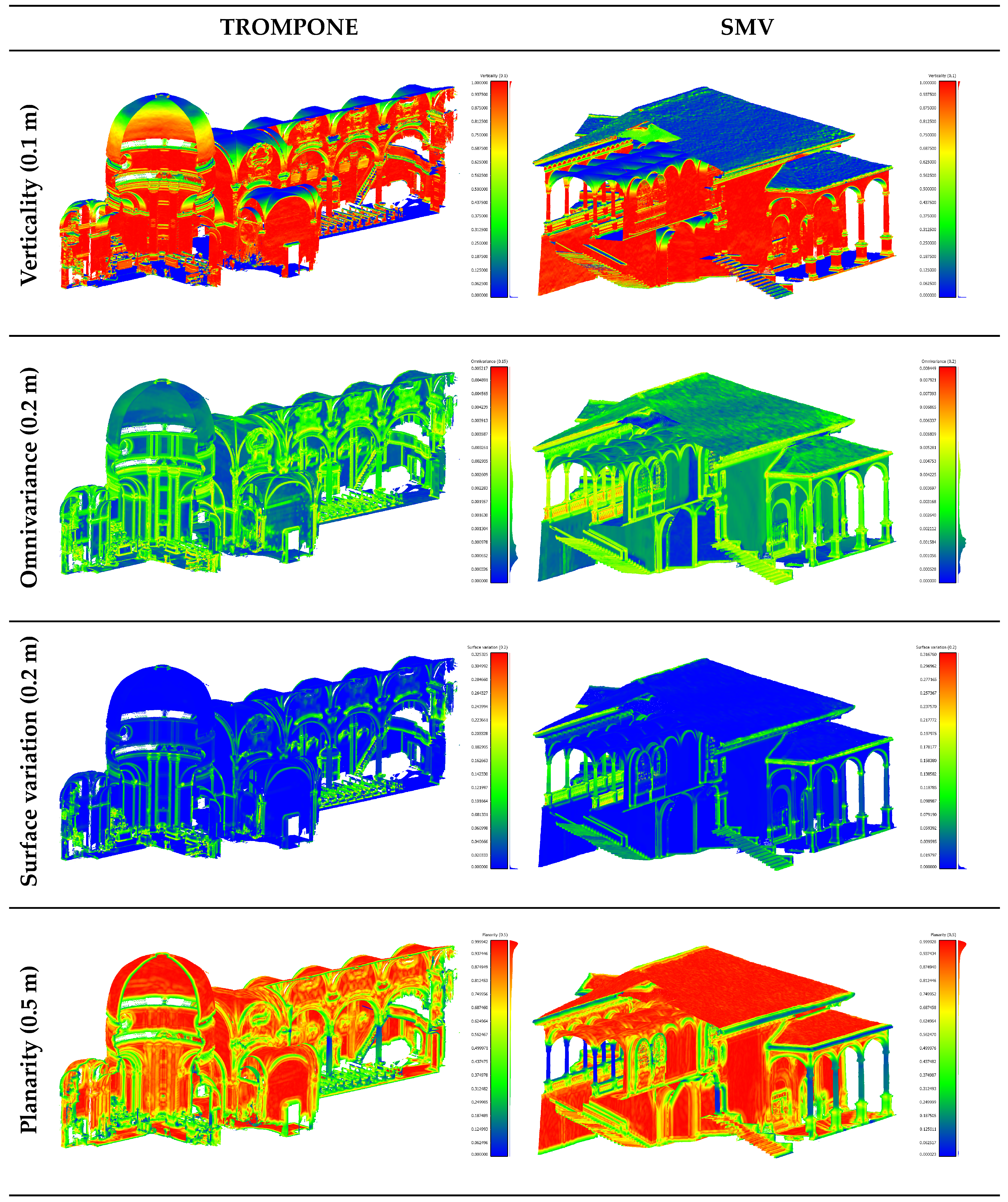
In order to effectively train the different ML classifiers a composition of 3D geometric features have been used, including normal-based (Verticality), height-based (Z coordinates), and eigenvalue-based features (also defined covariance features).

The covariance features [48] are shape descriptors obtained as a combination of eigenvalues (${\lambda }_1>{\lambda }_2>{\lambda }_3$) which are extracted from the covariance matrix, a 3D tensors that describe the distribution of point within a certain neighbourhood. Through statistical analysis, the Principal Component Analysis (PCA), it is possible to extract from this matrix the three eigenvalues representing the local 3D structure. According to Weinmann et al. [49], different strategies can be applied to recover the local neighbourhood for points belonging to a 3D point cloud. It can generally be computed as a sphere or a cylinder with a fixed radius or be described by the number of the kNN. In this paper, considering the studies presented in [24,25], only a few covariance features (Omnivariance, Surface Variation and Planarity) have been calculated on spherical neighbourhoods at specific radii in order to highlight the architectural components.

As one can see in Figure 2, different features emphasises different elements. Verticality makes easier the distinction between vertical and horizontal surfaces, allowing the recognition of walls and columns as well as floors, stairs and vaults. The feature planarity becomes useful for isolating columns and cylindrical elements if extracted at radii close to the diameter dimensions. Finally, surface variation and omnivariance, calculated within a short radius, emphasises changes in shapes facilitating, for example, the detection of moldings and windows.

3.3. Deep Learning for Point Cloud Semantic Segmentation

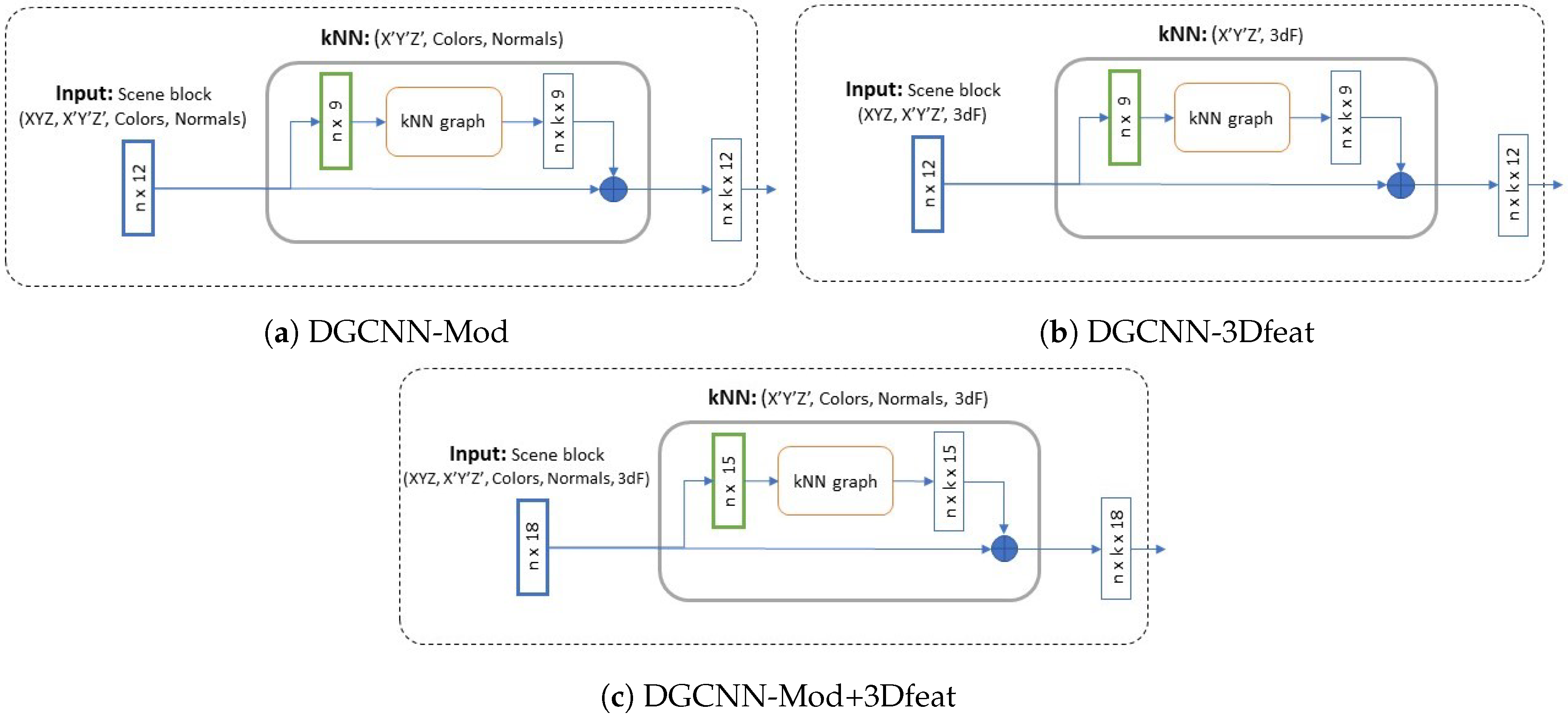
In this paper, the approach presented in [18] is adopted, where a modified version of DGCNN is proposed, called DGCNN-Mod. This implementation includes several improvements, compared to the original version: in the input layer, kNN phase considers coordinates of normalised points, color features transformations like HSV, and normal vectors. Moreover, the performance of the DGCNN-Mod is compared with two novel versions of this network: the DGCNN-3Dfeat and the DGCNN-Mod+3Dfeat that take into consideration other important features aforementioned. In particular, the DGCNN-3Dfeat adds to the kNN the 3D features. Instead, for a complete ablation study the DGCNN-Mod+3Dfeat comprises all the available features. Figure 3 represents the configurations of the EdgeConv layer with the various feature combinations.

Compared to the DGCNN-Mod, two types of pre-processing techniques are tested: Scaler1 and Scaler2. The Scaler1 standardises features by removing the mean and scaling to unit variance. The standard score of a sample x is determined as:

$$z=\frac{x-\mu }{\sigma }$$

(1)

where $\mu$ is the mean of the training samples and $\sigma$ is the standard deviation of the training samples. Instead, Scaler2 scales features using statistics that are robust to outliers. This pre-processing phase removes the median and scales the data according to the quantile range (IQR: InterQuartile Range). The IQR is the range between the 1st quartile (25th quantile) and the 3rd quartile (75th quantile). Centering and scaling happen independently on each feature by computing the relevant statistics on the samples in the training set. Median and interquartile range are then stored to be used on the validation and test set. In addition, the original DGCNN network uses the Cross Entropy Loss. Since we are using really unbalanced datasets, we decide to test Focal Loss [50] as well. This particular function has been implemented just to solve unbalance issues.

All deep learning approaches have been implemented using Python 3 and the well-known framework called Tensorflow. Pre-processing techniques on features, i.e., Scaler1 and Scaler2, have been implemented through the Scikit-Learn library [46], also implemented in Python.

3.4. Performance Evaluation Metrics

In the experimental section (Section 4), the employed state-of-the-art approaches are compared using the most common performance metrics for semantic segmentation. The Overall Accuracy (OA), along with weighted Precision, Recall and F1-Score are calculated regarding the test set, as these are very good performance indicators to understand if the approaches are able to generalise in a proper way. Please consider that OA and Recall have the same values, since the metrics are weighted. In addition, a comparison is also made between the individual classes of the test set, for each experiment performed: Precision, Recall, F1-Score and Intersection over Union (IoU) values are calculated for each type of object (see the Appendix A).

It is worth noting that, in the scenes to be classified, the number of points varies according to the two approaches involved. In fact, with ML the total number of points both in the input and output scene are used, while with DL the unseen point cloud is subsampled with respect to the original one, for computational reasons. The number of subsampled points could be arbitrarily set, the most used is 4096 for each analysed block, but higher values can be chosen (e.g., 8192) at training time expense. In this paper 4096 points per block have been set as subsampling parameter.

4. Results

In this section, several experiments performed with the previously presented ML and DL methods are reported. The experiment proposed in Section 4.1 regards the segmentation of the Trompone symmetrical scene, starting from the partial annotation of the same scene. In the second and third experiments, the training samples change according to the adopted classification strategy (ML or DL). Still, the same scenes are tested: SMV scene for Section 4.2 and SMG scene for Section 4.3.

4.1. First Experiment—Segmentation of a Partially Annotated Scene

In this setting, the Trompone scene is initially split into two parts, choosing one side for the training and the symmetrical one for the test. Then, the side used for the training phase is further split into training set (80%) and validation set (20%). The validation set is used to test the OA at the end of each training epoch while the evaluation is performed on the test set. For this test, nine architectural classes have been considered. Unlike the next experiments (Section 4.2 and Section 4.3), the class “Other” was used during the training as it could be uniquely identified with the furnishing of the church (mainly benches and confessionals). No points from the class "roof" were tested, this being an indoor scene.

Original DGCNN uses its standard hyper-parameters: normalised XYZ coordinates for the kNN phase and XYZ + RGB for the feature learning phase, with $1\times 1$ m block size. This latter parameter defines only the size of the block base, since the height is considered “endless”; in this way the whole scene can be analysed and the lowest number of blocks is defined. For the other DGCNN-based approaches we used the Scaler1 pre-processing setting for the features, as it resulted to be the best configuration among all the various tests performed. In addition, for the DGCNN-Mod+3Dfeat network, the best result was achieved using Focal Loss function.

In

Table 2. Weighted metrics computed for the Test set of the Trompone scene divided into 3 parts: Training, Validation, Test.

Model	Overall Accuracy	Precision	Recall	F1-Score
kNN	0.7438	0.7337	0.7438	0.7345
NB	0.6639	0.6406	0.6639	0.6364
DT	0.8345	0.8313	0.8345	0.8312
RF	0.8804	0.8796	0.8804	0.8754
DGCNN	0.7117	0.7400	0.7117	0.7040
DGCNN-Mod	0.7313	0.7344	0.7313	0.6963
DGCNN-3Dfeat	0.8723	0.8705	0.8723	0.8676
DGCNN-Mod+3Dfeat	0.8290	0.8271	0.8290	0.8215

, the performances of the state-of-the-art approaches are reported. As we can see, the best returns in terms of accuracy metrics come from the RF approach. In addition, the other approaches exceeding 0.80 of accuracy are DT, DGCNN-3Dfeat, and DGCNN-Mod+3Dfeat, which all have in common the use of the 3D features. We can, therefore, deduce that this type of features allows for an improvement of the original DGCNN performances as they are very representative for the classes under investigation.

Table A1. The Trompone scene has been divided into 3 parts: training, validation and test. In this Table we can see the metrics for every class, calculated on the test set.

Model	Metrics	Arch	Col	Mold	Floor	Do-Wi	Wall	Stair	Vault	Furnit
kNN	Precision	0.6813	0.6225	0.5474	0.941	0.2874	0.7116	0.5263	0.8255	0.7406
	Recall	0.4734	0.6975	0.5041	0.9698	0.197	0.7339	0.0349	0.9168	0.8026
	F1-Score	0.5587	0.6579	0.5248	0.9552	0.2338	0.7226	0.0654	0.8688	0.7704
	IoU	0.3876	0.4902	0.3558	0.9142	0.1324	0.5657	0.0338	0.768	0.6265
NB	Precision	0.5217	0.5914	0.416	0.8559	0.0812	0.5836	0.6672	0.7853	0.6891
	Recall	0.3384	0.8159	0.1898	0.9263	0.013	0.8625	0.0963	0.7993	0.6288
	F1-Score	0.4105	0.6857	0.2607	0.8897	0.0224	0.6961	0.1683	0.7922	0.6575
	IoU	0.2582	0.5218	0.1499	0.8013	0.0113	0.5339	0.0919	0.6559	0.4898
DT	Precision	0.8476	0.8924	0.7513	0.9661	0.3544	0.8021	0.4796	0.9113	0.7894
	Recall	0.6983	0.8696	0.7317	0.9731	0.2843	0.8099	0.1598	0.9422	0.8767
	F1-Score	0.7657	0.8809	0.7414	0.9696	0.3155	0.806	0.2397	0.9265	0.8307
	IoU	0.6204	0.7871	0.589	0.941	0.1873	0.6751	0.1362	0.8631	0.7105
RF	Precision	0.9207	0.9618	0.8562	0.9723	0.6054	0.8332	0.9661	0.9346	0.8259
	Recall	0.7694	0.8938	0.8066	0.9860	0.2707	0.8776	0.1519	0.9565	0.9321
	F1-Score	0.8383	0.9265	0.8307	0.9791	0.3741	0.8548	0.2626	0.9454	0.8758
	IoU	0.7216	0.8631	0.7103	0.9590	0.2301	0.7463	0.1511	0.8964	0.7790
DGCNN	Precision	0.4295	0.5789	0.5341	0.9604	0.4120	0.6606	0.4627	0.9121	0.5011
	Recall	0.4793	0.6174	0.3877	0.9743	0.1635	0.3767	0.0483	0.7832	0.9452
	F1-Score	0.4530	0.5975	0.4493	0.9673	0.2341	0.4798	0.0874	0.8428	0.6550
	IoU	0.2928	0.4260	0.2897	0.9366	0.1325	0.3156	0.0457	0.7282	0.4869
DGCNN- Mod	Precision	0.4448	0.1633	0.6177	0.9662	0.4082	0.6483	0.7121	0.8043	0.6462
	Recall	0.5763	0.6328	0.2484	0.9837	0.0771	0.1860	0.1730	0.9199	0.9602
	F1-Score	0.5021	0.2596	0.3543	0.9749	0.1297	0.2891	0.2784	0.8582	0.7725
	IoU	0.3352	0.1491	0.2153	0.9509	0.0693	0.1689	0.1616	0.7516	0.6293
DGCNN- 3Dfeat	Precision	0.7380	0.9154	0.7269	0.9847	0.4078	0.7413	0.9660	0.9544	0.8657
	Recall	0.7493	0.8757	0.6207	0.9845	0.1531	0.8620	0.3320	0.9207	0.9251
	F1-Score	0.7436	0.8951	0.6696	0.9846	0.2226	0.7971	0.4941	0.9373	0.8944
	IoU	0.5918	0.8101	0.5033	0.9696	0.1252	0.6627	0.3281	0.8819	0.8090
DGCNN- Mod+3Dfeat	Precision	0.5767	0.6834	0.7042	0.9782	0.4990	0.7492	0.9764	0.9044	0.7791
	Recall	0.6257	0.9305	0.4455	0.9870	0.1479	0.7811	0.2844	0.8867	0.9254
	F1-Score	0.6002	0.7881	0.5458	0.9826	0.2282	0.7648	0.4405	0.8954	0.8460
	IoU	0.4287	0.6502	0.3752	0.9657	0.1287	0.6191	0.2824	0.8106	0.7330

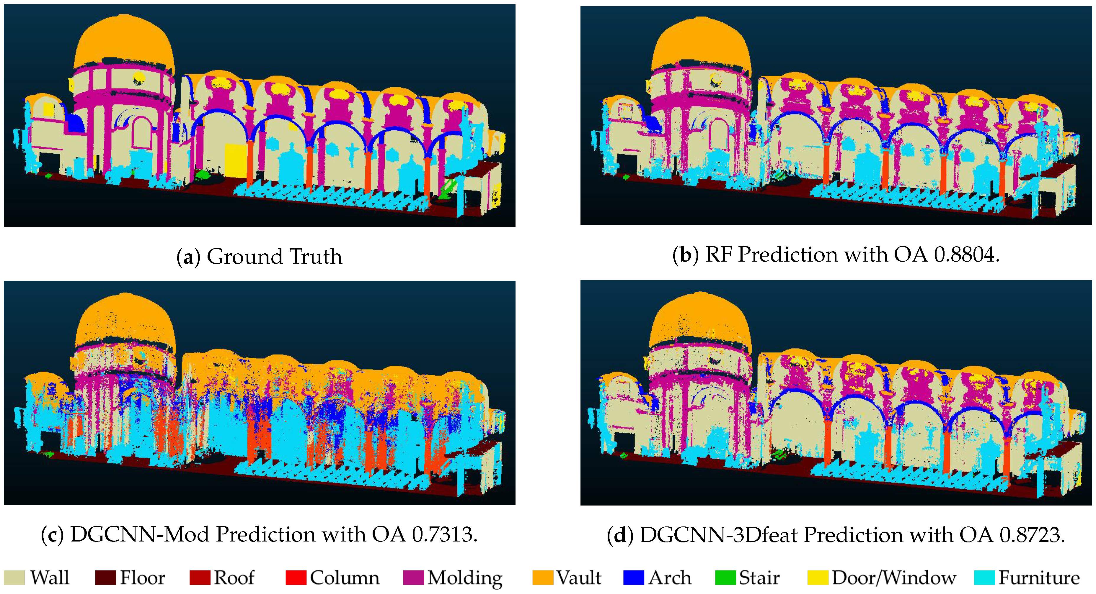
(see Appendix A) reports the accuracy metrics (Precision, Recall, F1-Score and IoU) for each class of the Trompone’s test set. From the analysis of this table it is possible to understand which are the classes that are best discriminated by the various approaches. Finally, Figure 4 depicts the manually annotated test scene (ground truth) and the automatic segmentation results, obtained with best approaches. From this visual result we can notice again the issues with the class Stair (in green), and Window-Door (in yellow) (e.g., in none of the approaches it has been possible to identify the door at the center of the scene).

4.2. Second Experiment—Segmentation of an Unseen Scene, the Sacro Monte Varallo (SMV)

In the second and third experiments, as previously anticipated, the training samples change according to the classification strategy adopted (ML or DL). Moreover, based on the experience of [30], the class "Other" is excluded from the classification, as the objects included are too variegated and it would confuse the NN. The portion of scene used to train the different ML classifiers consists of $\mathrm{2,526,393}$ points out of $\mathrm{16,200,442}$ points (approx. 16%) (Figure 5), while for the NNs 12 scenes of ArCH dataset have been used according to the previous tests performed in [18].

Same state-of-the-art approaches as in the previous section are evaluated.

In

Table 3. Weighted metrics computed for the Test set of the SMV scene.

Model	Overall Accuracy	Precision	Recall	F1-Score
kNN	0.8102	0.8588	0.8102	0.8248
NB	0.7331	0.7970	0.7331	0.7584
DT	0.8041	0.8522	0.8041	0.8180
RF	0.8369	0.8736	0.8369	0.8467
DGCNN	0.5608	0.6850	0.5608	0.5602
DGCNN-Mod	0.8294	0.8216	0.8295	0.8192
DGCNN-3Dfeat	0.7890	0.7776	0.7890	0.7720
DGCNN-Mod+3Dfeat	0.8452	0.8287	0.8452	0.8343

, the overall performances are reported for each tested model, while

Table A2. Tests performed on the SMV scene. For the DL approach 10 scenes as training, 1 for validation (5_SMV_chapel_1) and 1 for test.

Model	Metrics	Arch	Col	Mold	Floor	Do-Wi	Wall	Stair	Vault	Roof
kNN	Precision	0.3113	0.8476	0.3978	0.9522	0.0986	0.9701	0.7496	0.8645	0.8063
	Recall	0.5513	0.9458	0.6424	0.9147	0.4504	0.7632	0.8545	0.87	0.9402
	F1-Score	0.3979	0.894	0.4913	0.9331	0.1618	0.8543	0.7986	0.8673	0.8682
	IoU	0.2484	0.8084	0.3257	0.8746	0.088	0.7456	0.6647	0.7656	0.767
NB	Precision	0.0923	0.4263	0.2584	0.7577	0.0063	0.9515	0.7387	0.7486	0.8492
	Recall	0.233	0.8622	0.3506	0.7923	0.0121	0.7954	0.6896	0.744	0.764
	F1-Score	0.1322	0.5706	0.2975	0.7746	0.0083	0.8665	0.7133	0.7462	0.8043
	IoU	0.0708	0.3991	0.1748	0.6321	0.0042	0.7644	0.5544	0.5952	0.6727
DT	Precision	0.2618	0.8864	0.4637	0.9141	0.1251	0.9744	0.7784	0.8411	0.7528
	Recall	0.5676	0.9184	0.6194	0.857	0.5875	0.7654	0.8355	0.8549	0.9557
	F1-Score	0.3584	0.9021	0.5303	0.8846	0.2063	0.8574	0.8059	0.8479	0.8422
	IoU	0.2183	0.8217	0.3609	0.7932	0.115	0.7503	0.675	0.736	0.7275
RF	Precision	0.3586	0.8906	0.4738	0.9650	0.2058	0.9774	0.7873	0.8955	0.7795
	Recall	0.6262	0.9352	0.6557	0.9162	0.7115	0.7897	0.8605	0.9101	0.9747
	F1-Score	0.4560	0.9124	0.5501	0.9399	0.3193	0.8736	0.8223	0.9027	0.8662
	IoU	0.2953	0.8388	0.3794	0.8867	0.1899	0.7755	0.6982	0.8227	0.7640
DGCNN	Precision	0.1406	0.0134	0.1270	0.6641	0.2319	0.7496	0.6302	0.5267	0.8445
	Recall	0.0877	0.0004	0.4843	0.8050	0.2501	0.8797	0.0983	0.8757	0.3735
	F1-Score	0.1081	0.0007	0.2013	0.7278	0.2406	0.8095	0.1700	0.6578	0.5179
	IoU	0.0571	0.0003	0.1119	0.5721	0.1367	0.6799	0.0929	0.4900	0.3494
DGCNN- Mod	Precision	0.1145	0.7903	0.4249	0.7775	0.4171	0.7946	0.8271	0.8282	0.9420
	Recall	0.0543	0.0630	0.4138	0.8571	0.2376	0.9203	0.5938	0.8904	0.9238
	F1-Score	0.0737	0.1167	0.4193	0.8154	0.3028	0.8528	0.6913	0.8582	0.9328
	IoU	0.0382	0.0619	0.2652	0.6883	0.1784	0.7434	0.5281	0.7516	0.8740
DGCNN- 3Dfeat	Precision	0.2581	0.8243	0.3491	0.8052	0.1767	0.7761	0.8837	0.5968	0.9148
	Recall	0.1054	0.1029	0.1473	0.7578	0.0533	0.9074	0.7553	0.8719	0.8735
	F1-Score	0.1496	0.1830	0.2072	0.7808	0.0819	0.8367	0.8145	0.7086	0.8937
	IoU	0.0808	0.1007	0.1155	0.6404	0.0427	0.7192	0.6870	0.5487	0.8078
DGCNN- Mod+3Dfeat	Precision	0.1345	0.7007	0.4678	0.8302	0.4664	0.7950	0.8836	0.8528	0.9271
	Recall	0.0608	0.4260	0.3021	0.8311	0.3372	0.8874	0.7928	0.8578	0.9670
	F1-Score	0.0838	0.5299	0.3671	0.8307	0.3914	0.8386	0.8357	0.8553	0.9466
	IoU	0.0437	0.3604	0.2248	0.7104	0.2433	0.7221	0.7177	0.7471	0.8986

(see Appendix A) reports detailed results on the individual classes of the test scene. Original DGCNN is trained again using its standard hyperparameters. For the other DGCNN-based approaches we achieved the best results using:

• Focal Loss for DGCNN-Mod;
• Scaler1 pre-processing for DGCNN-3Dfeat;
• Focal loss and Scaler2 pre-processing for DGCNN-Mod+3Dfeat;

Table 3 shows that DGCNN-Mod+3Dfeat is the best approach in terms of OA, reaching 0.8452 on the Test Scene, followed by the RF with 0.8369. However, studying the results of the individual classes through Table A2, we can see that with the DL approach, two classes have not been well recognised (i.e., Arch and Column). The second best approach, on the contrary, gets better results on these classes, while maintaining an high average accuracy. 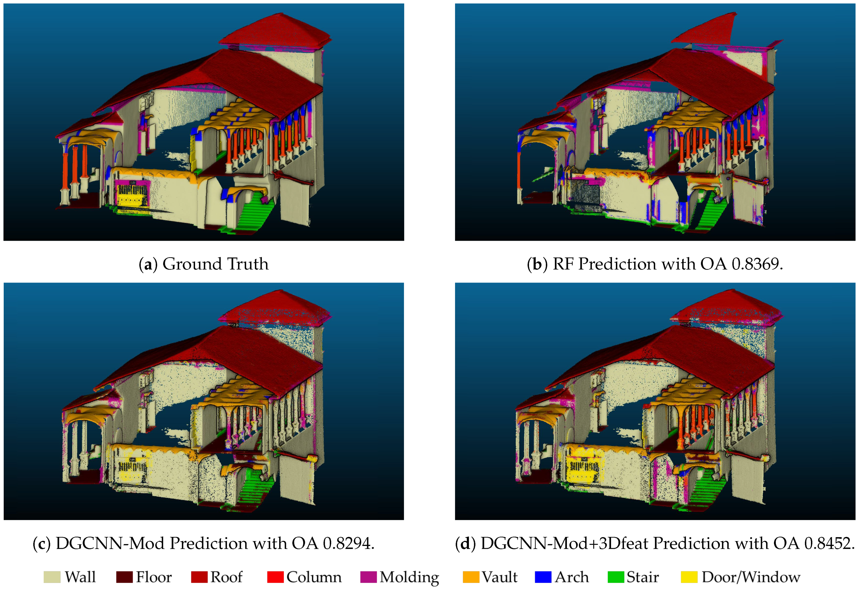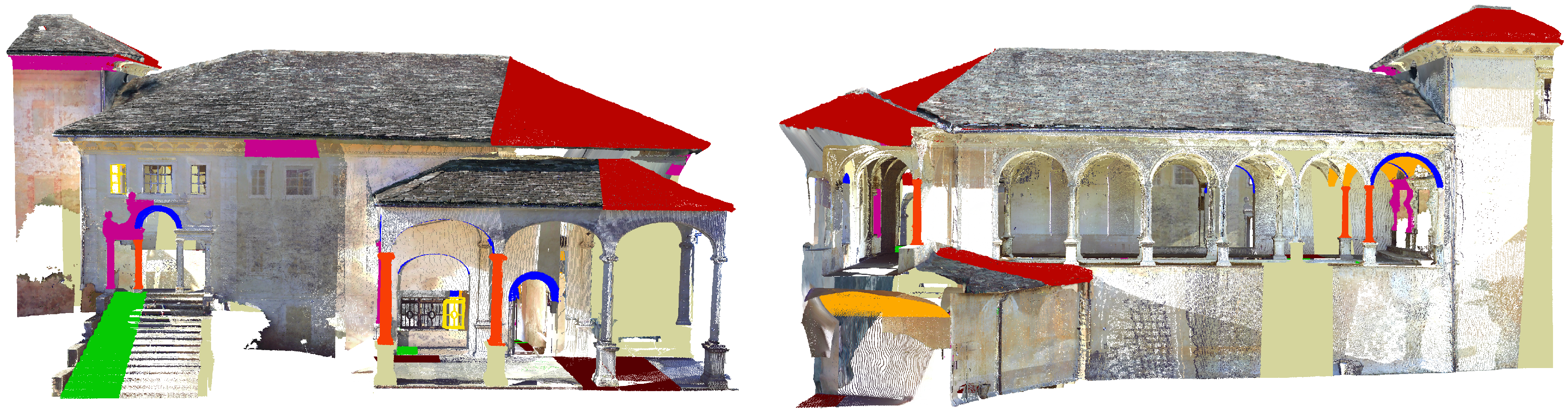Figure 6 depicts the manually annotated test scene (ground truth) and the automatic segmentation results obtained with the best approaches. It is possible to notice that most of the classes have been well recognised, except for the Arch class in the DGCNN-based approaches and the Door-Window class for the RF.

4.3. Third Experiment—Segmentation of an unseen scene, the Sacro Monte Ghiffa (SMG)

As in the previous experiments, for the ML approaches ad hoc annotations have been distributed along the point cloud (Figure 7), consisting of 3,545,900 points over a total of 17,798,049 points (approx. 20%).

In

Table 4. Weighted metrics computed for the Test set of the SMG scene.

Model	Overall Accuracy	Precision	Recall	F1-Score
kNN	0.6078	0.6565	0.6078	0.6262
NB	0.7186	0.7967	0.7186	0.7422
DT	0.8952	0.9014	0.8952	0.8971
RF	0.9266	0.9239	0.9266	0.9243
DGCNN	0.8514	0.8528	0.8514	0.8474
DGCNN-Mod	0.8951	0.8887	0.8951	0.8860
DGCNN-3Dfeat	0.8736	0.8887	0.8737	0.8776
DGCNN-Mod+3Dfeat	0.9135	0.9165	0.9135	0.9125

, the overall performances are reported for each tested model, while

Table A3. Tests performed on the SMG scene. For the DL approach 10 scenes as training, 1 for validation (5_SMV_chapel_1) and 1 for test.

Model	Metrics	Arch	Col	Mold	Floor	Do-Wi	Wall	Stair	Vault	Roof
kNN	Precision	0.0797	0.1083	0.2245	0.741	0.1122	0.6433	0.1048	0.6796	0.8658
	Recall	0.1515	0.2466	0.3676	0.5441	0.0754	0.6135	0.0522	0.7501	0.7345
	F1-Score	0.1044	0.1505	0.2788	0.6275	0.0902	0.6281	0.0696	0.7131	0.7948
	IoU	0.0551	0.0814	0.162	0.4572	0.0472	0.4578	0.0361	0.5541	0.6594
NB	Precision	0.2961	0.6661	0.389	0.9708	0.0518	0.8684	0.2194	0.5621	0.9177
	Recall	0.3855	0.9163	0.3498	0.9177	0.3581	0.7205	0.6014	0.8871	0.6382
	F1-Score	0.335	0.7714	0.3684	0.9435	0.0905	0.7876	0.3215	0.6882	0.7528
	IoU	0.2012	0.6279	0.2258	0.893	0.0474	0.6496	0.1916	0.5246	0.6036
DT	Precision	0.3748	0.6723	0.2467	0.9293	0.1100	0.7348	0.3416	0.7929	0.9681
	Recall	0.0766	0.1736	0.1379	0.8466	0.3084	0.8823	0.3442	0.8737	0.9439
	F1-Score	0.1272	0.2759	0.1769	0.8860	0.1621	0.8018	0.3429	0.8314	0.9559
	IoU	0.0679	0.1601	0.0970	0.7953	0.0882	0.6692	0.2069	0.7114	0.9154
RF	Precision	0.6911	0.9480	0.7750	0.9670	0.3842	0.9210	0.7320	0.9281	0.9834
	Recall	0.8507	0.9857	0.7304	0.9525	0.1072	0.9424	0.7415	0.9684	0.9605
	F1-Score	0.7620	0.9665	0.7520	0.9597	0.1677	0.9316	0.7367	0.9478	0.9718
	IoU	0.6155	0.9351	0.6026	0.9225	0.0915	0.8718	0.5831	0.9008	0.9451
DGCNN	Precision	0.3748	0.6723	0.2467	0.9293	0.1100	0.7348	0.3416	0.7929	0.9681
	Recall	0.0766	0.1736	0.1379	0.8466	0.3084	0.8823	0.3442	0.8737	0.9439
	F1-Score	0.1272	0.2759	0.1769	0.8860	0.1621	0.8018	0.3429	0.8314	0.9559
	IoU	0.0679	0.1601	0.0970	0.7953	0.0882	0.6692	0.2069	0.7114	0.9154
DGCNN- Mod	Precision	0.4581	0.7928	0.5973	0.9196	0.1080	0.7740	0.4392	0.8895	0.9799
	Recall	0.1685	0.5478	0.2241	0.8662	0.0708	0.9417	0.4487	0.9066	0.9851
	F1-Score	0.2464	0.6479	0.3260	0.8921	0.0856	0.8497	0.4439	0.8980	0.9825
	IoU	0.1404	0.4791	0.1947	0.8051	0.0446	0.7386	0.2852	0.8148	0.9655
DGCNN- 3Dfeat	Precision	0.4986	0.8980	0.6102	0.9425	0.1004	0.8444	0.4884	0.6890	0.9717
	Recall	0.2006	0.8216	0.4907	0.8772	0.2753	0.8326	0.6128	0.9813	0.9314
	F1-Score	0.2860	0.8581	0.5440	0.9087	0.1471	0.8384	0.5435	0.8096	0.9511
	IoU	0.1668	0.7514	0.3736	0.8326	0.0794	0.7217	0.3731	0.6800	0.9068
DGCNN- Mod+3Dfeat	Precision	0.6479	0.7626	0.6659	0.9669	0.2183	0.8377	0.4799	0.8870	0.9839
	Recall	0.1840	0.9255	0.4974	0.8937	0.3681	0.8910	0.6317	0.9794	0.9831
	F1-Score	0.2866	0.8362	0.5695	0.9289	0.2741	0.8635	0.5455	0.9309	0.9835
	IoU	0.1672	0.7184	0.3980	0.8672	0.1588	0.7598	0.3750	0.8706	0.9675

(see Appendix A) reports detailed results on the individual classes of the test scene. Best results have been achieved with RF, immediately followed by the DGCNN-Mod+3Dfeat network. However, in this case, given the higher symmetry of the point cloud, if compared to the SMV scene, the increase in OA when using the 3D features is lower, but still significant. Results are consistent with the previous test and the most problematic class is again the Door-Window, probably due to the dataset unbalance.

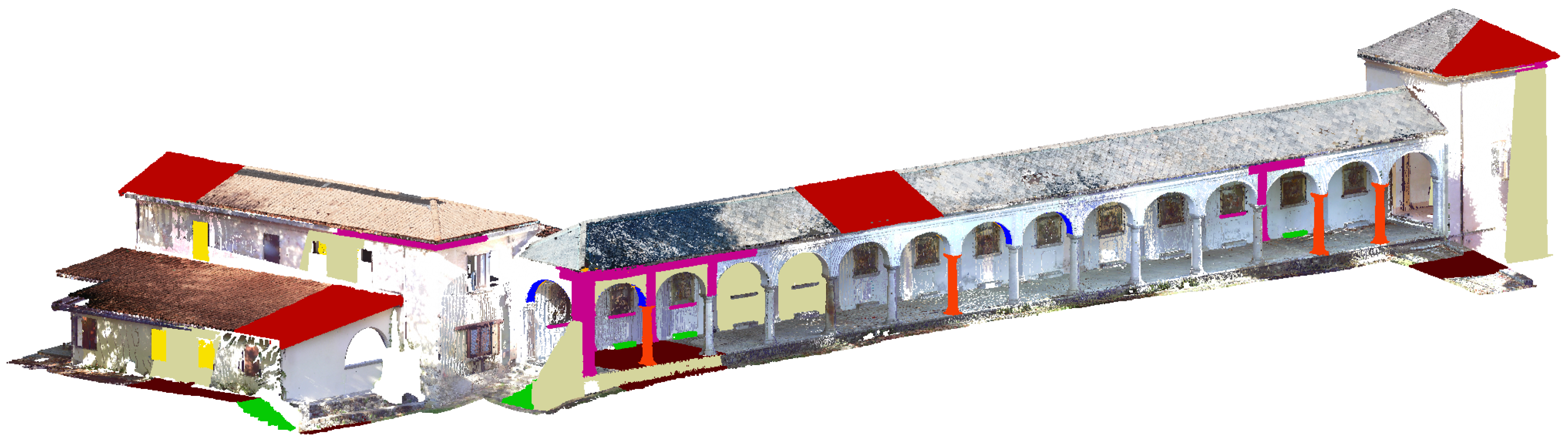
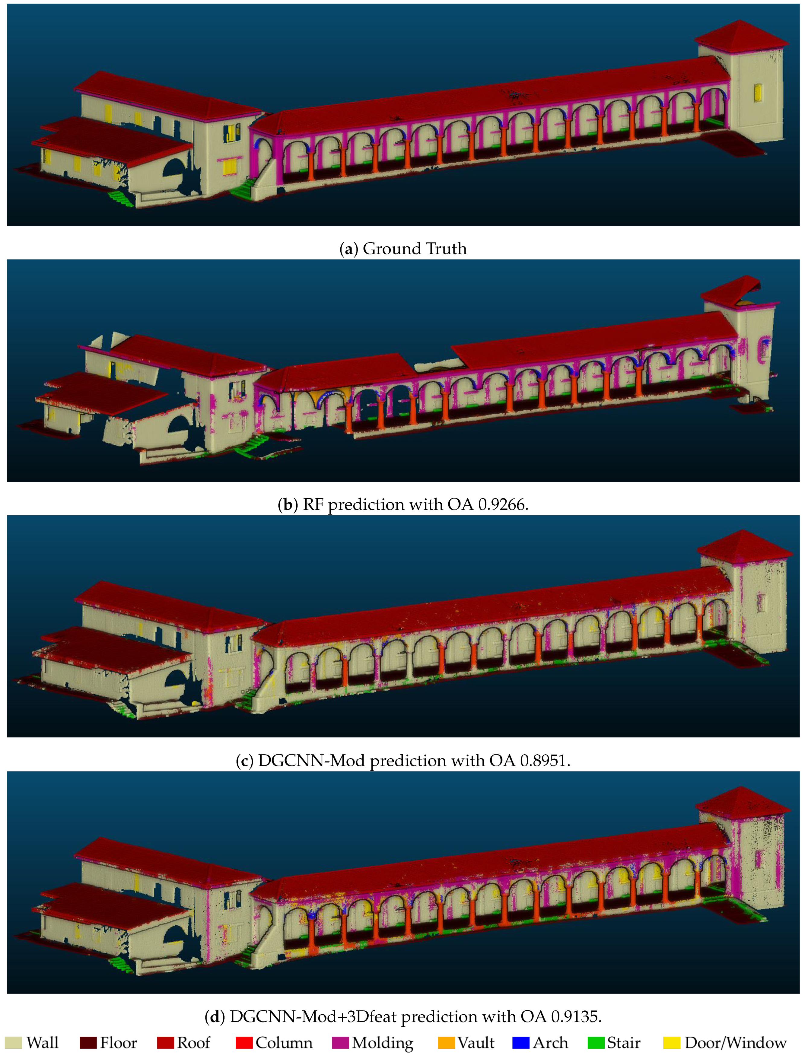
Finally, Figure 8 depicts the manually annotated test scene (ground truth) and the automatic segmentation results obtained with best approaches.

4.4. Results Analysis

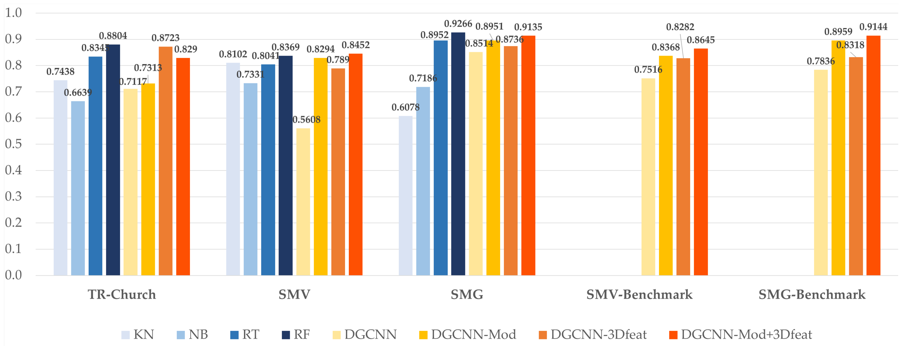
The recap of the best OA achieved (Figure 9) highlights that the Random Forest method is slightly better in the two almost symmetrical scenes of Ghiffa and the Trompone church. In these cases, with manual annotation, it is possible to select a number of adequately representative examples of the test scene, ensuring an accurate result. The DL solutions, on the other hand, seem to work better in the non-symmetric scene, thus showing a good generalisation ability. More generally, the results of DL are satisfactory, as they demonstrate the achievement of OA similar to those of RF, although the training set is partially limited, if compared to the others present in the state of the art.

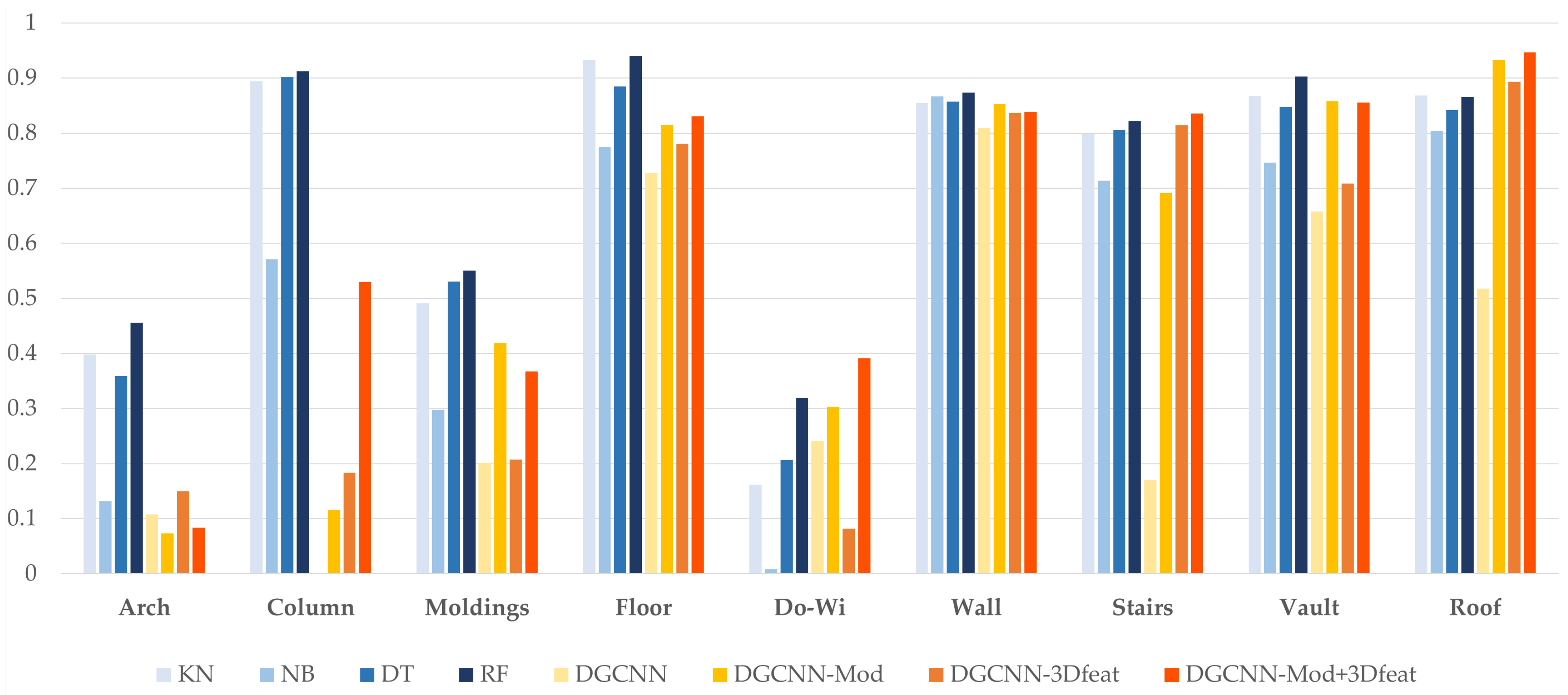
Figure 10 shows the F1-Score, a combination of precision and recall, relative to the single classes. In this case, the ML approaches outperform DL for some classes such as Arch, Column, Molding and Floor, while the DL gives better results in the segmentation of Door-Window and Roof. The remaining classes of Vault, Wall and Stair are equally balanced between the results of the two techniques, with vaults and walls leaning towards the RF and stairs to the DGCNN-Mod+3Dfeat.

5. Discussions

Answering to the first research question (RQ1), it can be said that nowadays it is possible to provide best practices for semantic segmentation of point clouds in the CH domain. In fact, the tests conducted and the results described above show that the introduction of 3D features has led to an increase in OA, if compared to the simple use of radiometric components and normals. This increase is about 10% in the tests on the symmetric scene (Trompone church), while it is lower (approximately 2%) in the tests run with different scenes as training and SMV or SMG as tests. In the latter case, however, the introduction of the 3D features, associated with the use of the normals and the RGB features, has improved the recognition of the classes with fewer points and which, previously, resulted with lower metrics (for example Column, Door-Window and Stair). As it is possible to notice in Table A1, Table A2 and Table A3, for all the approaches, the worst recognised classes are Arch, Door-Window and, alternatively, Molding or Stair. This result is likely due to the fact that these are the classes with the lowest number of points within the scenes.

A similar conclusion can be made for the introduction of the focal loss, which, with the same hyperparameters configuration, has led to an increase of the performance for the Molding, Door-Window, and Stair classes.

With regard to RQ2, experiment results show that RF outperformed the other ML classifiers. At the same time, the best DL results have been achieved with the combination of all the selected features, without leading to an increase in computational time. Previous tests, not presented here, highlighted that what actually affects this latter aspect is the block size and the number of subsampled points.

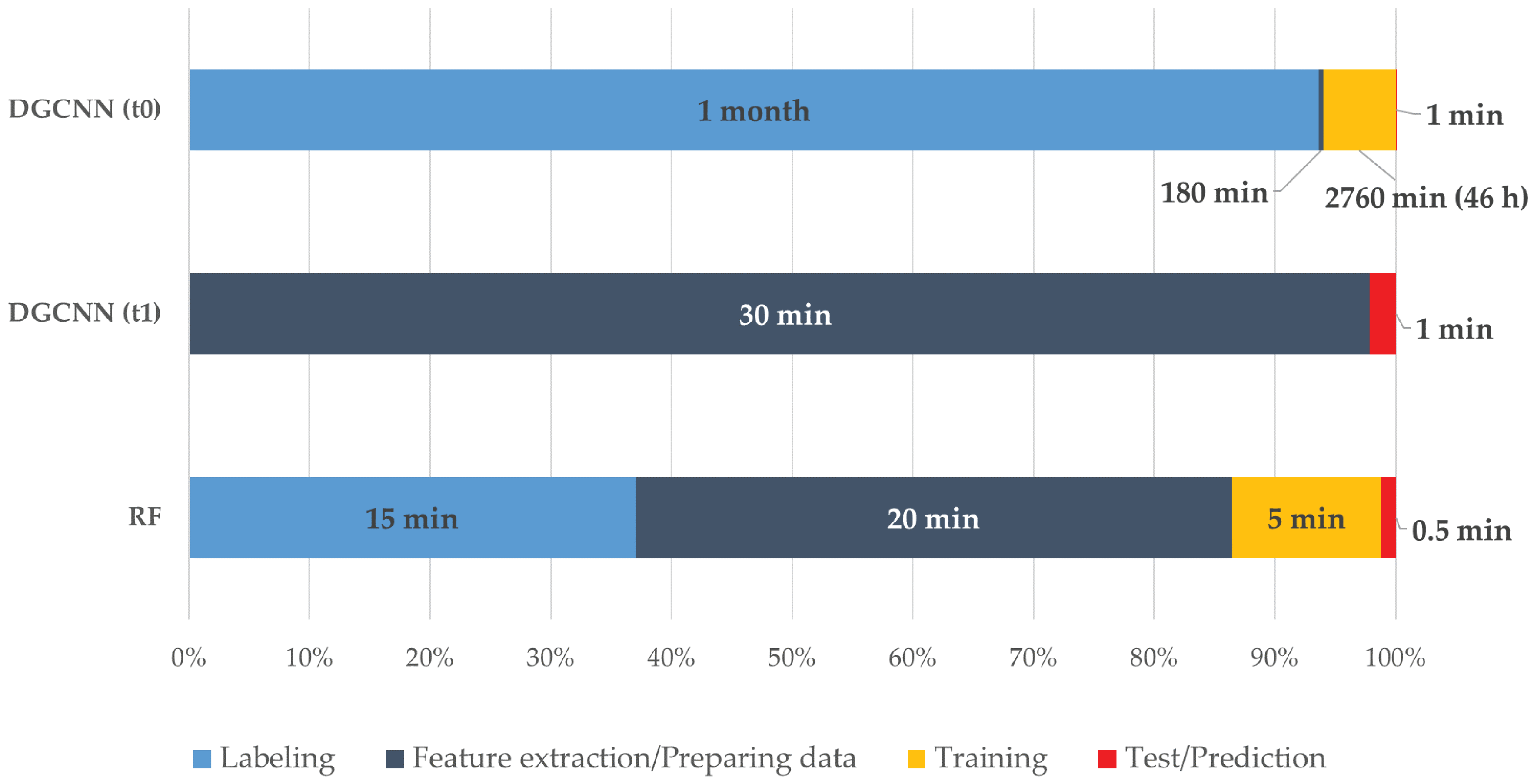
Talking about RQ3, as described in the results section, the authors think that there is still no winning solution between the ML and DL approaches. The OA of the best ML method and the DL one differs slightly. However, contrasting results are highlighted if the classes are analysed individually, where approaches could be chosen according to the needs. Both techniques have strengths and weaknesses. In the case of ML, there is a customisation of the training set according to the scene to be predicted, very useful in the CH domain, while for the DL there is the possibility of cutting out the manual annotation, further automating the process. Another element to take into consideration when comparing machine and deep learning approaches is the processing time. If the ML pipeline is well defined, within the DL framework, it is necessary to make a distinction between two possible scenarios which considerably differ in times. In the first scenario, when an annotated training set is not available, it is necessary to manually label as many scenes as possible (a very time-consuming task), pre-process the data (e.g., subsampling, normals computation, centering on the 0,0,0 point, block creation, etc.), then wait for the training phase from a few hours to a few days. In the second scenario, it is possible to start from saved weights of a network which had been pre-trained on a released benchmark (ArCH in this case), and directly proceed to the preparation and test of the new scene, without any manual annotation phase. So, depending on whether one compares the RF with the first or second scenario, the balance needle can tip in favor of one or the other technique. In Figure 11, a comparison between the times required for the tests carried out in this paper is shown. It must be considered that ML tests were run on an Nvidia GTX 1050 TI 8 GB, 32 GB RAM, processor Intel(R) Xeon(R) CPU E5-1650 0 @ 3.20 GHz, while for the DL an Nvidia RTX 2080 TI 11 GB, 128 GB RAM, processor Intel(R) Xeon(R) Silver 4214 CPU @ 2.20 GHz was used.

Finally, regarding RQ4, it is fair to state that the main drawback in the comparison between different algorithms is the limited similarity of their pipeline. In fact, a proper comparison between algorithms would necessarily require the same input and/or output. As regards the input, considering the different nature of the algorithms, this would mean giving to the ML classifiers a huge amount of annotated data which would compromise its performances, or viceversa training the neural network with a few data compared to that required. For this reason, in order to analyse the best classification approaches for heritage scenarios, we preferred to use different training scenes for the ML and DL input. Concerning the output, for the DL approach an interpolation with the initial scene should be conducted for a comparison with the same number of points, leading to a likely OA decrease. However, as the subsampling operation is mainly due to computational reasons, easily solved in the near future with more and more performing machines, the usefulness of the interpolation would certainly be reduced and become even pointless. Moreover, using different interpolation algorithms would introduce a further element of error making the pipeline less objective and reproducible.

6. Conclusions and Future Works

This study explored semantic segmentation of complex 3D point clouds in the CH domain. To do so, ML techniques and DL techniques have been compared exploiting a novel and previously unexplored benchmark dataset.

Both ML and DL algorithms proved to be valuable, having great potential for classifying datasets collected with different Geomatics techniques (e.g., LiDAR and photogrammetric data). When comparing the performances of both approaches, it appears that there is not a winning solution, classifiers had similar overall performances, and none of them outperformed each other. Even considering the single classes studied for the experiments, it emerges that the different approaches are alternatively better depending on the class analysed, but none of the methods attained a result able to generally outperform all the classes.

In general terms, the training time of classical ML techniques can be up to one order of magnitude smaller; conversely, a small but noteworthy improvement in performance could be witnessed for DL techniques over classical ML techniques, considering the whole benchmark dataset (Table A4). In ML, hyperparameter optimization or tuning is the problem of choosing a set of optimal hyperparameters for a learning algorithm. Its value is used to control the process of learning. Instead, DL techniques have the advantage of allowing more additional experimentation with the model setup. Using DL techniques on a dataset of this size and for this type of problem therefore shows promise, especially in performance critical applications. On the other side, the DL model is largely influenced by the processes of tuning the structural parameters both in computational cost and operational time. However, given that state-of-the-science large-scale inventories are moving towards deep learning-based classifications, we can expect that in the upcoming future the growing availability of training dataset will overcome such limitation. The feature engineering and feature extraction are key, and time consuming parts of the ML workflow, since these phases transforming training data and augmenting it with additional features in order to make ML algorithms more effective. DL has been changing this process and deep neural networks have been explored as black-box modelling strategies.

The final legacy of this work, which was aimed at opening a positive debate among the different involved domain experts, is summarised in

Table 5. Comparative overview table with the key differences between the two proposed frameworks in the CH domain. From low (*) to high (***).

	Machine Learning	Deep Learning
Training Set Size Dependencies	*	***
Programming Skills	*	***
Feature Engineering	***	*
Algorithm Structure	*	***
Interpretability	***	*
Training Time	*	**
Hyperparameter Tuning	***	***
Processing Power and Expensive hardware (GPUs)	**	***

, where pros and cons of both ML/DL methods are summarised.

References

- Yu, H.; Yang, Z.; Tan, L.; Wang, Y.; Sun, W.; Sun, M.; Tang, Y. Methods and datasets on semantic segmentation: A review. Neurocomputing 2018, 304, 82–103. [Google Scholar] [CrossRef]
- Zhang, K.; Hao, M.; Wang, J.; de Silva, C.W.; Fu, C. Linked dynamic graph CNN: Learning on point cloud via linking hierarchical features. arXiv 2019, arXiv:1904.10014. [Google Scholar]
- Xie, Y.; Tian, J.; Zhu, X. A Review of Point Cloud Semantic Segmentation. IEEE Geosci. Remote Sens. Mag. (GRSM) 2020. [Google Scholar] [CrossRef] [Green Version]
- Llamas, J.; M Lerones, P.; Medina, R.; Zalama, E.; Gómez-García-Bermejo, J. Classification of architectural heritage images using deep learning techniques. Appl. Sci. 2017, 7, 992. [Google Scholar] [CrossRef] [Green Version]
- Grilli, E.; Özdemir, E.; Remondino, F. Application of machine and deep learning strategies for the classification of heritage point clouds. Int. Arch. Photogramm. Remote Sens. Spat. Inf. Sci. 2019, XLII-4/W18, 447–454. [Google Scholar] [CrossRef] [Green Version]
- Grilli, E.; Remondino, F. Classification of 3D Digital Heritage. Remote Sens. 2019, 11, 847. [Google Scholar] [CrossRef] [Green Version]
- Malinverni, E.; Pierdicca, R.; Paolanti, M.; Martini, M.; Morbidoni, C.; Matrone, F.; Lingua, A. Deep learning for semantic segmentation of 3D point cloud. Int. Arch. Photogramm. Remote Sens. Spat. Inf. Sci. 2019, XLII-2/W15, 735–742. [Google Scholar] [CrossRef] [Green Version]
- Pierdicca, R.; Mameli, M.; Malinverni, E.S.; Paolanti, M.; Frontoni, E. Automatic Generation of Point Cloud Synthetic Dataset for Historical Building Representation. In Proceedings of the International Conference on Augmented Reality, Virtual Reality and Computer Graphics, Santa Maria al Bagno, Italy, 24–27 June 2019; pp. 203–219. [Google Scholar]
- LeCun, Y.; Bengio, Y.; Hinton, G. Deep learning. Nature 2015, 521, 436–444. [Google Scholar] [CrossRef]
- Klokov, R.; Lempitsky, V. Escape from cells: Deep kd-networks for the recognition of 3d point cloud models. In Proceedings of the IEEE International Conference on Computer Vision, Venice, Italy, 22–29 October 2017; pp. 863–872. [Google Scholar]
- Xie, S.; Liu, S.; Chen, Z.; Tu, Z. Attentional shapecontextnet for point cloud recognition. In Proceedings of the IEEE Conference on Computer Vision and Pattern Recognition, Salt Lake City, UT, USA, 18–23 June 2018; pp. 4606–4615. [Google Scholar]
- Altman, N.S. An introduction to kernel and nearest-neighbor nonparametric regression. Am. Stat. 1992, 46, 175–185. [Google Scholar]
- Zhang, H. Exploring conditions for the optimality of naive Bayes. Int. J. Pattern Recognit. Artif. Intell. 2005, 19, 183–198. [Google Scholar] [CrossRef]
- Breiman, L.; Friedman, J.; Stone, C.J.; Olshen, R.A. Classification and Regression Trees; CRC Press: Boca Raton, FL, USA, 1984. [Google Scholar]
- Breiman, L. Random forests. Mach. Learn. 2001, 45, 5–32. [Google Scholar] [CrossRef] [Green Version]
- Wang, Y.; Sun, Y.; Liu, Z.; Sarma, S.E.; Bronstein, M.M.; Solomon, J.M. Dynamic graph cnn for learning on point clouds. ACM Trans. Graph. (TOG) 2019, 38, 1–12. [Google Scholar] [CrossRef] [Green Version]
- Matrone, F.; Lingua, A.; Pierdicca, R.; Malinverni, E.S.; Paolanti, M.; Grilli, E.; Remondino, F.; Murtiyoso, A.; Landes, T. A benchmark for large-scale heritage point cloud semantic segmentation. ISPRS Int. Arch. Photogramm. Remote Sens. Spat. Inf. Sci. 2020, XLIII-B2, 1419–1426. [Google Scholar] [CrossRef]
- Pierdicca, R.; Paolanti, M.; Matrone, F.; Martini, M.; Morbidoni, C.; Malinverni, E.S.; Frontoni, E.; Lingua, A.M. Point Cloud Semantic Segmentation Using a Deep Learning Framework for Cultural Heritage. Remote Sens. 2020, 12, 1005. [Google Scholar] [CrossRef] [Green Version]
- Oses, N.; Dornaika, F.; Moujahid, A. Image-based delineation and classification of built heritage masonry. Remote Sens. 2014, 6, 1863–1889. [Google Scholar] [CrossRef] [Green Version]
- Riveiro, B.; Lourenço, P.B.; Oliveira, D.V.; González-Jorge, H.; Arias, P. Automatic morphologic analysis of quasi-periodic masonry walls from LiDAR. Comput. Aided Civ. Infrastruct. Eng. 2016, 31, 305–319. [Google Scholar] [CrossRef]
- Barsanti, S.G.; Guidi, G.; De Luca, L. Segmentation of 3D models for cultural heritage structural analysis–some critical issues. ISPRS Ann. Photogramm. Remote Sens. Spatial Inf. Sci. 2017, 4, 115. [Google Scholar] [CrossRef] [Green Version]
- Poux, F.; Neuville, R.; Hallot, P.; Billen, R. Point cloud classification of tesserae from terrestrial laser data combined with dense image matching for archaeological information extraction. Int. J. Adv. Life Sci. 2017, 4, 203–211. [Google Scholar] [CrossRef] [Green Version]
- Grilli, E.; Dininno, D.; Marsicano, L.; Petrucci, G.; Remondino, F. Supervised segmentation of 3D cultural heritage. In Proceedings of the 2018 3rd Digital Heritage International Congress (DigitalHERITAGE) held jointly with 2018 24th International Conference on Virtual Systems & Multimedia (VSMM 2018), San Francisco, CA, USA, 26–30 October 2018; pp. 1–8. [Google Scholar]
- Grilli, E.; Farella, E.; Torresani, A.; Remondino, F. Geometric features analysis for the classification of cultural heritage point clouds. Int. Arch. Photogramm. Remote Sens. Spatial Inf. Sci. 2019, XLII-2/W15, 541–548. [Google Scholar] [CrossRef] [Green Version]
- Grilli, E.; Remondino, F. Machine Learning Generalisation across Different 3D Architectural Heritage. ISPRS Int. J. Geo-Inf. 2020, 9, 379. [Google Scholar] [CrossRef]
- Murtiyoso, A.; Grussenmeyer, P. Virtual Disassembling of Historical Edifices: Experiments and Assessments of an Automatic Approach for Classifying Multi-Scalar Point Clouds into Architectural Elements. Sensors 2020, 20, 2161. [Google Scholar] [CrossRef] [Green Version]
- Zhang, J.; Zhao, X.; Chen, Z.; Lu, Z. A Review of Deep Learning-based Semantic Segmentation for Point Cloud (November 2019). IEEE Access 2019, 7, 179118–179133. [Google Scholar] [CrossRef]
- Griffiths, D.; Boehm, J. SynthCity: A large scale synthetic point cloud. arXiv 2019, arXiv:1907.04758. [Google Scholar]
- Qi, C.R.; Su, H.; Mo, K.; Guibas, L.J. Pointnet: Deep learning on point sets for 3d classification and segmentation. In Proceedings of the IEEE Conference on Computer Vision and Pattern Recognition, Honolulu, HI, USA, 21–26 July 2017; pp. 652–660. [Google Scholar]
- Qi, C.R.; Yi, L.; Su, H.; Guibas, L.J. Pointnet++: Deep hierarchical feature learning on point sets in a metric space. In Proceedings of the 31st Conference on Neural Information Processing Systems (NIPS 2017), Long Beach, CA, USA, 4–9 December 2017; pp. 5099–5108. [Google Scholar]
- Atzmon, M.; Maron, H.; Lipman, Y. Point convolutional neural networks by extension operators. arXiv 2018, arXiv:1803.10091. [Google Scholar] [CrossRef] [Green Version]
- De Deuge, M.; Quadros, A.; Hung, C.; Douillard, B. Unsupervised feature learning for classification of outdoor 3d scans. In Proceedings of the Australasian Conference on Robitics and Automation, Sydney, NSW, Australia, 2–4 December 2013; Volume 2, p. 1. [Google Scholar]
- Armeni, I.; Sener, O.; Zamir, A.R.; Jiang, H.; Brilakis, I.; Fischer, M.; Savarese, S. 3d semantic parsing of large-scale indoor spaces. In Proceedings of the IEEE Conference on Computer Vision and Pattern Recognition, Las Vegas, NV, USA, 27–30 June 2016; pp. 1534–1543. [Google Scholar]
- Geiger, A.; Lenz, P.; Stiller, C.; Urtasun, R. Vision meets robotics: The kitti dataset. Int. J. Robot. Res. 2013, 32, 1231–1237. [Google Scholar] [CrossRef] [Green Version]
- Hackel, T.; Savinov, N.; Ladicky, L.; Wegner, J.D.; Schindler, K.; Pollefeys, M. Semantic3d. net: A new large-scale point cloud classification benchmark. arXiv 2017, arXiv:1704.03847. [Google Scholar]
- Chen, B.; Shi, S.; Gong, W.; Zhang, Q.; Yang, J.; Du, L.; Sun, J.; Zhang, Z.; Song, S. Multispectral LiDAR point cloud classification: A two-step approach. Remote Sens. 2017, 9, 373. [Google Scholar] [CrossRef] [Green Version]
- Zhang, J.; Lin, X.; Ning, X. SVM-based classification of segmented airborne LiDAR point clouds in urban areas. Remote Sens. 2013, 5, 3749–3775. [Google Scholar] [CrossRef] [Green Version]
- Laube, P.; Franz, M.O.; Umlauf, G. Evaluation of features for SVM-based classification of geometric primitives in point clouds. In Proceedings of the IEEE 2017 Fifteenth IAPR International Conference on Machine Vision Applications (MVA), Nagoya, Japan, 8–12 May 2017; pp. 59–62. [Google Scholar]
- Babahajiani, P.; Fan, L.; Gabbouj, M. Object recognition in 3D point cloud of urban street scene. In Proceedings of the Asian Conference on Computer Vision, Singapore, 1–2 November 2014; pp. 177–190. [Google Scholar]
- Li, Z.; Zhang, L.; Tong, X.; Du, B.; Wang, Y.; Zhang, L.; Zhang, Z.; Liu, H.; Mei, J.; Xing, X.; et al. A three-step approach for TLS point cloud classification. IEEE Trans. Geosci. Remote Sens. 2016, 54, 5412–5424. [Google Scholar] [CrossRef]
- Lodha, S.K.; Fitzpatrick, D.M.; Helmbold, D.P. Aerial lidar data classification using adaboost. In Proceedings of the IEEE Sixth International Conference on 3-D Digital Imaging and Modeling (3DIM 2007), Montreal, QC, Canada, 21–23 August 2007; pp. 435–442. [Google Scholar]
- Liu, Y.; Aleksandrov, M.; Zlatanova, S.; Zhang, J.; Mo, F.; Chen, X. Classification of power facility point clouds from unmanned aerial vehicles based on adaboost and topological constraints. Sensors 2019, 19, 4717. [Google Scholar] [CrossRef] [Green Version]
- Kang, Z.; Yang, J.; Zhong, R. A bayesian-network-based classification method integrating airborne lidar data with optical images. IEEE J. Sel. Top. Appl. Earth Obs. Remote Sens. 2016, 10, 1651–1661. [Google Scholar] [CrossRef]
- Thompson, D.R.; Hochberg, E.J.; Asner, G.P.; Green, R.O.; Knapp, D.E.; Gao, B.C.; Garcia, R.; Gierach, M.; Lee, Z.; Maritorena, S.; et al. Airborne mapping of benthic reflectance spectra with Bayesian linear mixtures. Remote Sens. Environ. 2017, 200, 18–30. [Google Scholar] [CrossRef]
- Belgiu, M.; Drăguţ, L. Random forest in remote sensing: A review of applications and future directions. ISPRS J. Photogramm. Remote Sens. 2016, 114, 24–31. [Google Scholar] [CrossRef]
- Pedregosa, F.; Varoquaux, G.; Gramfort, A.; Michel, V.; Thirion, B.; Grisel, O.; Blondel, M.; Prettenhofer, P.; Weiss, R.; Dubourg, V.; et al. Scikit-learn: Machine learning in Python. J. Mach. Learn. Res. 2011, 12, 2825–2830. [Google Scholar]
- John, G.H.; Langley, P. Estimating continuous distributions in Bayesian classifiers. arXiv 2013, arXiv:1302.4964. [Google Scholar]
- Chehata, N.; Guo, L.; Mallet, C. Airborne lidar feature selection for urban classification using random forests. Laser Scanning 2009 IAPRS 2009, XXXVIII-3/W8, 207–212. [Google Scholar]
- Weinmann, M.; Jutzi, B.; Hinz, S.; Mallet, C. Semantic point cloud interpretation based on optimal neighborhoods, relevant features and efficient classifiers. ISPRS J. Photogramm. Remote Sens. 2015, 105, 286–304. [Google Scholar] [CrossRef]
- Lin, T.Y.; Goyal, P.; Girshick, R.; He, K.; Dollár, P. Focal loss for dense object detection. In Proceedings of the IEEE International Conference on Computer Vision, Venice, Italy, 22–29 October 2017; pp. 2980–2988. [Google Scholar]
Figure 1.
Workflow for the machine learning (ML) and deep learning (DL) framework comparison.
Figure 2.
Three-dimensional features used to train the ML and DL classifiers. The colour of the plot represents the feature scale. The used search radii are reported in brackets.
Figure 3.
Modified EdgeConv layer for DGCNN-based approaches.
Figure 4.
Ground Truth and predicted point clouds, by using best approaches on Trompone’s Test side.
Figure 5.
Manual annotations used to train the ML algortihms for the Sacro Monte Varallo (SMV) Scene.
Figure 6.
Section of Ground Truth (a) and the best Predictions (b–d) of the SMV scene. Please note that the point clouds deriving from the DL approach are subsampled.
Figure 7.
Manual annotations used to train the ML algortihms for the Sacred Mount of Ghiffa (SMG) Scene.
Figure 8.
Ground Truth (a) and the best Predictions (b–d) of the SMG scene. Please note that the point clouds deriving from the DL approach are subsampled.
Figure 9.
Overall Accuracy of all tests carried out.
Figure 10.
F1-Score of the different classes for the SMV scene with the different approaches.
Figure 11.
Normalised comparison of times required for the different scenarios test. NN (t0) represents the first scenario in which the whole dataset has been manually labeled and the DGCNN-based methods have been trained on all the scenes. NN (t1), on the other hand, represents the next scenario in which it is possible to use the weights from the pre-trained neural network and conduct directly the data preparation (feature extraction, scaling, blocks creation, subsampling...) and the final test for the prediction.