Article

Spatial Analysis of Settlement Structures to Identify Pattern Formation Mechanisms in Inter-Urban Systems

Chair of Fluid Systems, Technische Universität Darmstadt, Otto-Berndt-Straße 2, D-64287 Darmstadt, Germany
*
Author to whom correspondence should be addressed.
ISPRS Int. J. Geo-Inf. 2020, 9(9), 541; https://0-doi-org.brum.beds.ac.uk/10.3390/ijgi9090541
Submission received: 12 August 2020 / Revised: 2 September 2020 / Accepted: 7 September 2020 / Published: 8 September 2020
(This article belongs to the Special Issue Geodata Science and Spatial Analysis in Urban Studies)

Abstract

:
Dissipative structures known from non-equilibrium thermodynamics can form patterns. Cities are regarded as open, dissipative structures due to their self-organisation and thus in theory are also capable of pattern formation. In a first step to understand similarities between nonlinear pattern formation and inter-urban systems, we investigate how inter-urban structures are arranged. We use data from the Global Urban Footprint to identify spatial regularities in seven regions (Argentina, China, Egypt, France, India, Ghana and USA) and to quantitatively describe settlement patterns by number of objects and density. We find that small areas of the examined data sets show a regular arrangement, the density and number of settlements differ widely between the different regions and the portion of regular areas within this regions strongly correlates with these two parameters. The results can be used to develop mathematical models that describe inter-urban pattern formation on the one hand and to investigate to what extent the respective settlement patterns are related to infrastructural, economic or political boundary conditions on the other.

1. Introduction

Urbanisation coupled with major demographic transformations is, along with climate change, one of the most striking phenomena of the early 21st century [1] and has increasingly moved into the focus of scientific work in recent decades [2]. This development has led to a “science of cities” [3], where with the help of quantitative mathematical models, various attempts are made to gain access to the different processes that shape and change today’s cities [4,5].
A major focus is the investigation of urban morphology [6] and land use within cities and their surroundings. To describe and predict changes in land use, cellular automata are a commonly used tool [7]. In the last decades, these are extended by mobile agents, resulting in agent-based models describing the interaction between the actors and the respective environment they are operating in [8].
However, due to the integration of ever larger amounts of data [9], more complex algorithms [10], especially machine learning and deep learning, the models are becoming more and more complex [11]. The “black-box” structure of these models, coupled with an increasing number of nuances considered in the models, leads to a loss of comprehensibility [12]. A contrary approach is taken when certain phenomena are mapped with comparatively simple mathematical models to describe core processes of urbanisation.
A very famous model to describe urban structures was made by Walter Christaller in the early 1930s, when he developed the concept of the central place theory (CPT) [13]. This theory is based on the assumption that from a locally homogeneous distribution of small settlements, urban hierarchies develop over time in which larger towns take over certain infrastructural tasks for their neighbours. Although the theory has been criticised (see, e.g., in [14]), both the hierarchy in settlement structures for different regions [15] and the regularity in the arrangement of rural settlements [16] can be shown empirically.
While many models based on CPT focused on the development from regular to hierarchical structures [14], less attention was paid to the development of the initial regular structures. The only approach known to us following this direction for inter-urban system deals with the regular spatial arrangement of industrial plants. Paul Krugman [17] proposed that the regular spatial arrangement of these plants can be described by a diffusion-driven instability.
Besides diffusion-driven instability, other open thermodynamic systems can be found in nature that form regular structures such as the Taylor–Couette flow, Rayleigh–Benard convection and Benard–Maragoni convection. The order far from thermodynamic equilibrium arises by instabilities that grow, stimulated by small disturbances or imperfections [18]. As urban systems are also open systems [19], the question arises whether they can be described by nonlinear mathematical models of this type. In recent years, there have been increasing attempts to transfer these physical nonlinear models to intra-urban patterns or structures [20,21,22].
However, we are concerned with patterns in inter-urban systems. Qualitative different pattern of urban structures can be linked to the growth mechanisms urban sprawl [23,24] and sprinkling [25,26], which have social and ecological effects [23]. A deeper understanding of these patterns, processes and modelling possibilities [25,27] is therefore of great importance.
In a first step, we examine the nature of the structures formed by inter-urban systems on the basis of different examples in order to examine the applicability of these nonlinear models in future work with the knowledge that such an approach is only an indication of pattern formation mechanism [28]. Our research question is as follows.
How are settlements arranged in different predominantly rural regions of the world?
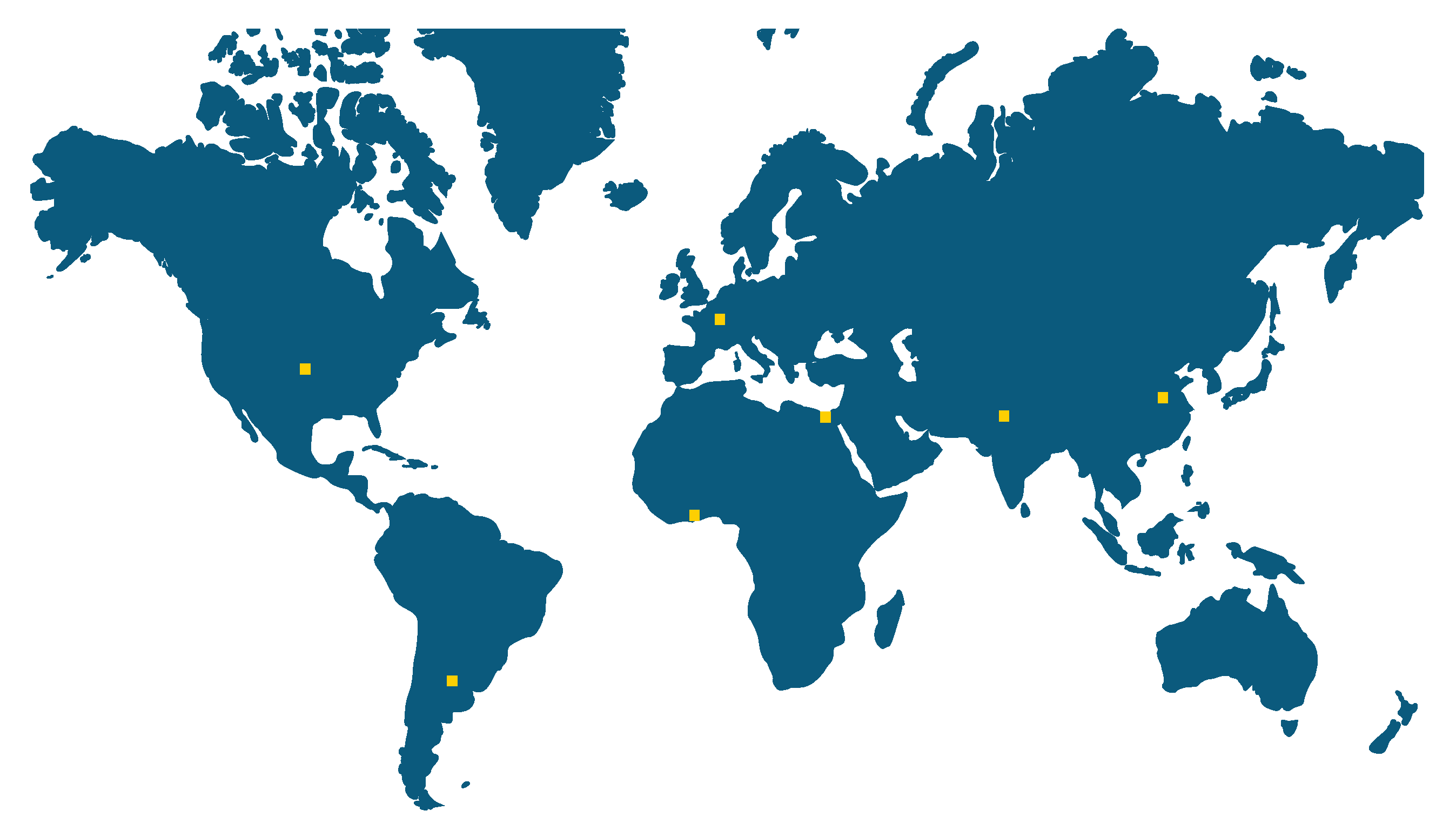
Although there are studies that examine the regularity of settlement arrangements [15,16], these are often not globally comparative. Therefore, we compare settlement patterns determined by satellite data in seven different regions of the world, using the following framework.

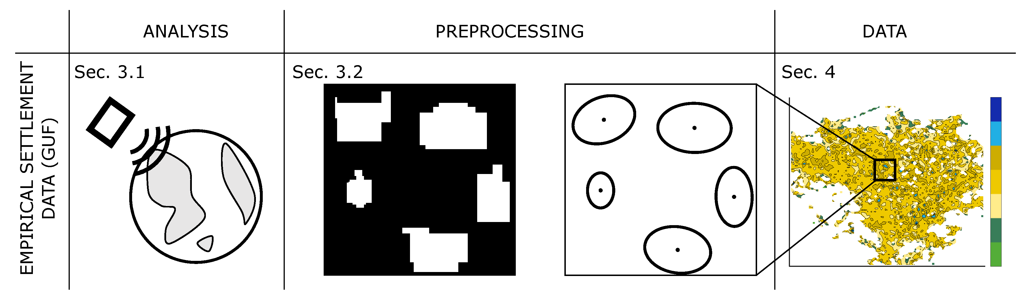
2. Conceptual Framework

Against the background of the strong spread of machine learning, a wide variety of scientific domains are concerned with patterns. In our analysis, we investigate two-dimensional binary patterns.
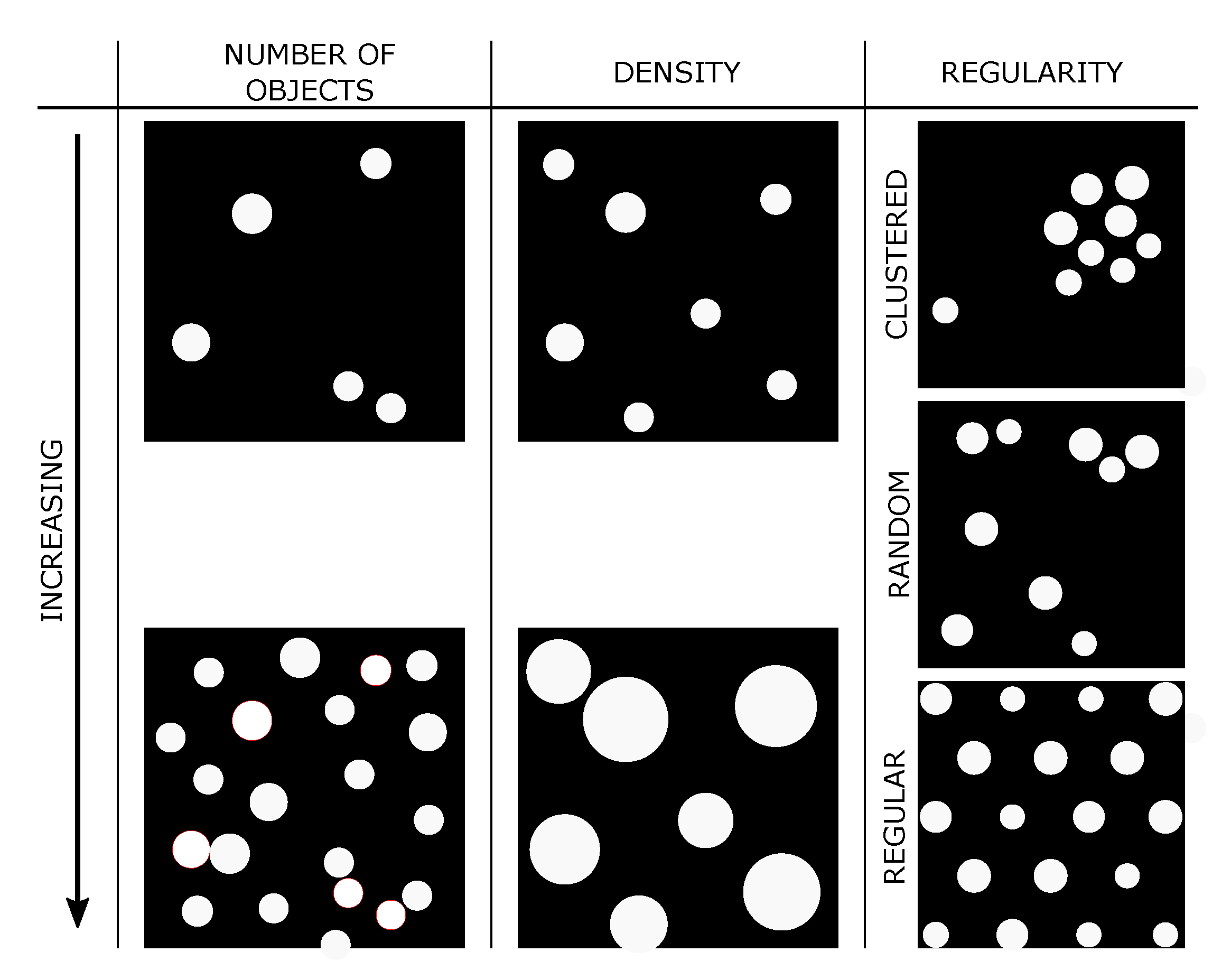
To answer the research questions stated above, consistent methods are in need. The properties of the settlement patterns have to be quantified in a correct yet condensed manner, to be able to compare settlement structures in different regions. Therefore, we use the following three parameters (Figure 1),
(i)
the number of objects investigated;
(ii)
the density of objects within the investigated area; and
(iii)
the regularity, which we quantify with a special characteristic value.
While the number and density represent continuous values from “low” to “high”, the regularity is divided into three classes. These are clustered, random and regular. In this procedure we neglect the shape of the individual objects. With these methods we quantify settlement patterns, using the framework in Figure 2.
We first present and briefly explain in Section 3 the empirical data and analysis methods used before we present the results in Section 4 and discuss them afterwards in Section 5.

3. Data and Methods

3.1. Data

As empirical data the GUF is used, a data set by the German Aerospace Center (DLR), which is based on data from the TanDEM-x mission. The data of the GUF are from the years 2011 and 2012. The radar data collected by the two satellites are evaluated fully automatically in three steps by the Urban Footprint Processor and a binary settlement map with a resolution of approximately 12 m is produced [29,30,31]. The binary settlement map thus consists of pixels of the resolution just mentioned, which indicate whether the respective area is settled or not.
In our analysis, we investigated sections from seven primarily agricultural regions on five continents, namely, regions in Argentina, China, Egypt, France, Ghana, India and USA, which all are equally sized with 200 km by 200 km (Figure 3). The coordinates of the data sets are given in the Table A1. Figure 4 shows examples of the GUF examined in China and Egypt. In this analysis, we focus on agricultural dominated landscapes as different settlement theories like the CPT [13] or others [32,33] are based on regular distribution of non-urban settlements as initial state. In selecting the regions, we have tried to obtain as comprehensive a picture as possible by examining countries with different economic development (developing and developed). In addition, as few metropolitan regions as possible should be present. Cairo (Egypt) is the exception, as the Nile Delta is a very interesting and otherwise a homogeneous settlement area north of the Sahara.

3.2. Method

As introduced in Section 2 the settlements patterns resulting from the GUF are examined with regard to the three dimensionless parameters, the number of objects N, density ϱ and the Average-Nearest Neighbour Index ( ANN ) as a measurement for regularity.
We define density as the quotient of the populated area A build - up and investigated area A:
ϱ : = A build - up A .
The ANN [34] is commonly used to measure the distribution of settlements in geographical investigations [15,16]. It distinguishes clustered, random and regular patterns, represented by ANN values near 0, 1 or 2.15 , respectively. When calculating the ANN , the arithmetic mean r ¯ A of the distance r i between every data point i [ 1 , N ] and its nearest neighbour in the investigated area A is used. This distance is compared to the distance r ¯ E = 0.5 A / N of data points in a random distribution [34]:
ANN = r ¯ A r ¯ E = 2 i = 1 N r i N · A
Similar to the work in [16], we differentiate between clustered ( 0 ANN 0.6 ), random ( 0.6 < ANN 1.5 ) and regular ( ANN > 1.5 ) distribution.
In order to quantify the reliability of the classification of the pattern as deviating from a regular distribution, the z-value for the ANN is calculated. It indicates the probability with which the hypothesis of a random point distribution can be rejected correctly. A z-value < 1.96 or > 1.96 forms the 90% confidence interval and the value is defined as
z = r ¯ A r ¯ E 0.26136 · N A
We first use the parameters introduced in Section 2, namely, number of objects N, density ϱ and ANN to describe the pattern of settlement arrangement. Calculating the A N N by considering all settlement objects in the area consisting of at least five pixels, we get a ANN < 1 for all data sets.
As this does not allow detailed analyses, the number of objects N, the density ϱ and the ANN are evaluated in sample squares spreading out on all seven investigated regions. For each analysis, the equally sized sample squares are equidistantly arranged in vertical and horizontal direction. The distance between adjacent sample squares is considerably less than their length of the edge. The distance is 0.5 km for sample square length equal to 2 km. 1 km for sample square length 3 km and larger sample squares have a distance of 2 km. Because squares crossing the border of the investigated area would result in misleading results, the sample squares are not covering the data set’s edges. The sample square’s result for N, ϱ and ANN are assigned to its centre to depict the results of each sample square for the entire data set.

4. Analysis

4.1. Settlement Arrangement
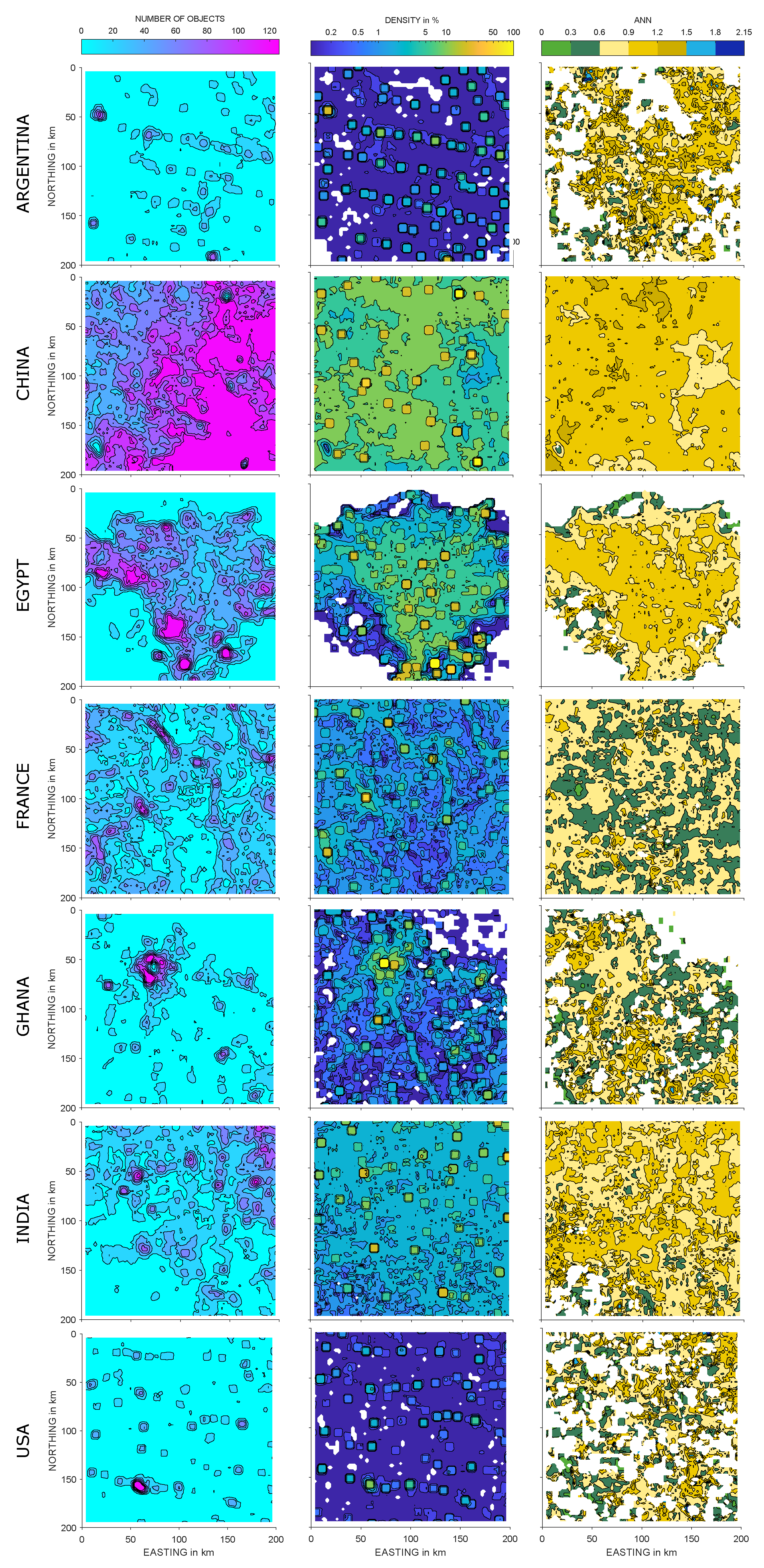
In Figure 5, the parameters N , ϱ and ANN for sample squares with a length of 8 km are shown.
It should be noted that the abstraction of the data in GUF to the centre of gravity and surface area of the object can lead to densities greater than 100%. This is the case when a large number of objects with a large size have their centre of gravity in the sample square, but their dimensions considerably exceed the sample square’s border. This results in a settlement area that is larger than the area of the sample square. We limit the value of density to 100%.
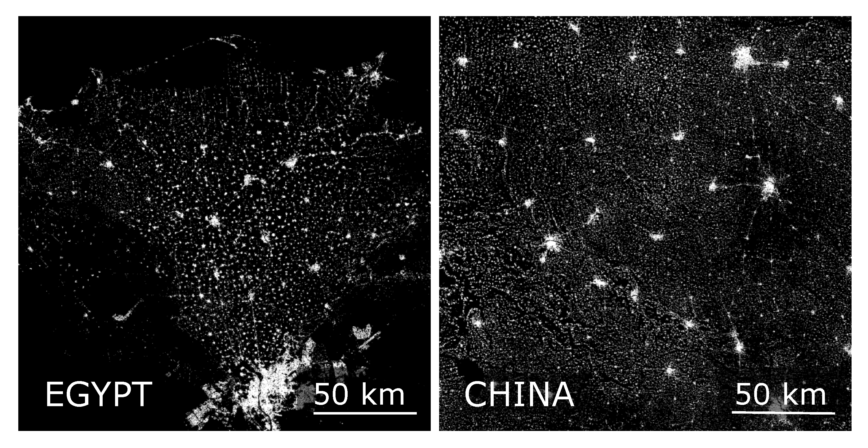
Figure 5 allows us to characterise each data set: Data set Argentina shows equidistant spots with higher levels of density, which belong to larger cities in the observed region. The southeastern corner in the data set China is characterised by high numbers of objects and low density, therefore representing small settlement objects. The settlements in the data set Egypt clearly follow the Nile Delta and the agglomeration of Cairo can be identified easily. The vein-shaped areas with low porosities that run through the data set France are characterised by rivers on whose banks a higher number of settlement objects can be found. In the data set Ghana, the clustering of settlement objects around the million city of Kumansi is clearly visible. Clusters of dense settlement structures are located in the north of the data set India, while the southern part contains very few settlement objects. The data set USA includes only a small number of objects, which have a small expansion. Therefore, the chosen sample square length is not suitable for ANN evaluation in this data set.
In every regions the clear majority of sample squares is characterised as random distribution by the ANN . Nevertheless, the individual data sets do have differences: In the data set Argentina, the majority of sample squares is represented by an ANN ranging from 0.6 to 1.2 ; in the data sets China and Egypt, most of the sample squares have an ANN greater 0.9 and smaller 1.2 ; in France, Ghana, India and USA, the dominating range is 0.6 < ANN 0.9 .
Nevertheless, in some regions a small percentage of squares, e.g., 2.7% in data set Argentina and 2.6% in data set USA, contain, according to the ANN , regular structures (see Table A2).
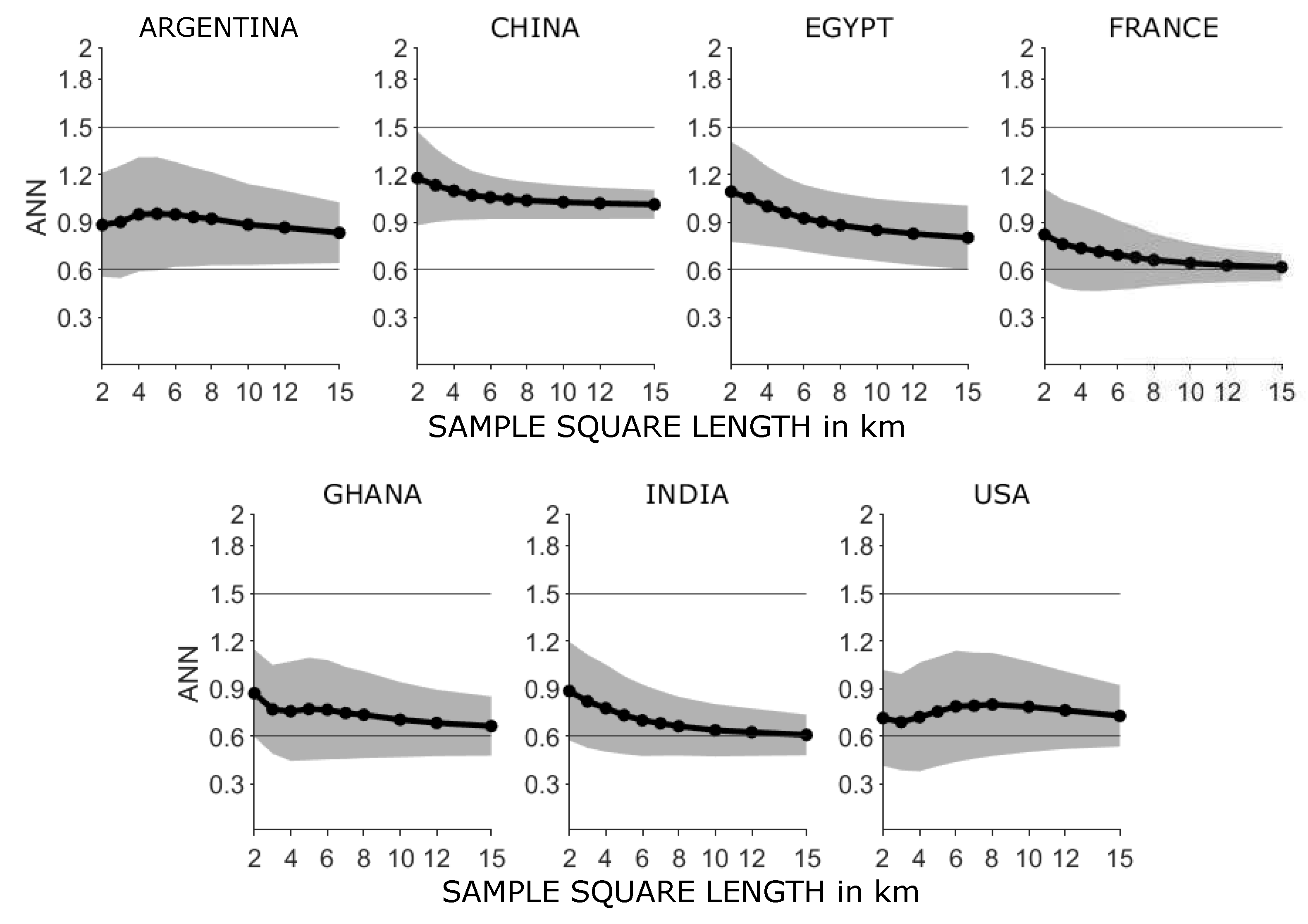
In order to investigate the arrangement of settlement objects in more detail, the described analysis with sample squares was repeated for squares with different edge lengths. The averaged results are shown in Figure 6. The effect of the sample squares’ size on the ANN becomes visible: With increasing edge length the ANN decreases, whereas in sparsely populated areas an increase to medium sample square edge lengths is detected before the decrease. It also becomes clear that the settlement objects in the data sets China and Egypt are more regularly distributed than the settlements in the other data sets.
However, sample squares with regular settlement distribution can be found for all data sets. For the share of regular sample squares in the each data refer to Table A2. While for a sample window size of 2 × 2 km 2 the proportion of windows with a A N N > 1.5 is between 0.8% (USA) and ~14% (China), for 3 × 3 km 2 between 0.95% (France) and 4% (India), for larger sample windows (15 × 15 km 2 ) the values are between 0 % for China and 0.23% for Argentina (Table A2). Areas of regular settlement structures can thus be observed above all in small settlement sections.
All sample squares listed with ANN > 1.5 result in a z-value above 1.96. In this case, the ANN delivers the reliable result of a non-random distribution.
The investigated regions show noticeable differences in terms of number of objects, density and portion of regular spots in the settlement structures. Nevertheless, similarities in the data sets Argentina and USA, and Egypt and India can be seen.

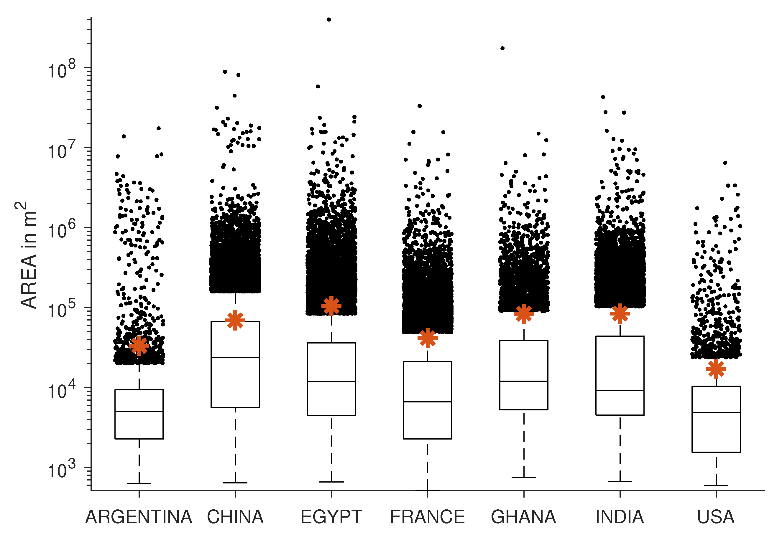
4.2. Size Distribution

To examine some of the points from above more closely, in addition to the three parameters N , ϱ and A N N , the the size distribution of the expansion of the settlement objects in all data sets was examined, see Figure 7. It is found that the median of all seven data sets is in a similar range of 10 4 m 2 , as well as the geometric mean S 0 given in Table 1. The characteristic size of the inter-urban structures investigated here is thus in the same range as the intra-urban structures of morphological slums investigated in [35,36].
It also becomes clear that there are few settlement objects to be found in the regions investigated in Argentina and the USA. In addition, these two data sets do not contain as many large settlement objects as the other investigated regions, and are very similar in this aspect. This fact does not seem surprising, as the data sets show a part of the Argentinean Pampas and the American Great Plains. In the following, these two areas are referred to as sparsely populated. The data set China contains by far the most settlement objects, which also have the largest extension. The data sets India and Egypt contain a similar number of objects and have a characteristic size of the objects, which differs only slightly. Both number and characteristic length range between the extremes of the sparsely populated data sets and the extremely dense populated data set China.
The data sets Ghana and France cannot be easily classified into the categories of sparsely, medium and densely populated areas. France has a similarly large number of objects as India and Egypt, but contains objects of much smaller dimensions, whereas in Ghana, the extent of the objects is comparable with the extent of the objects in the data set India and the number of objects is close to the number of sparsely populated data sets.
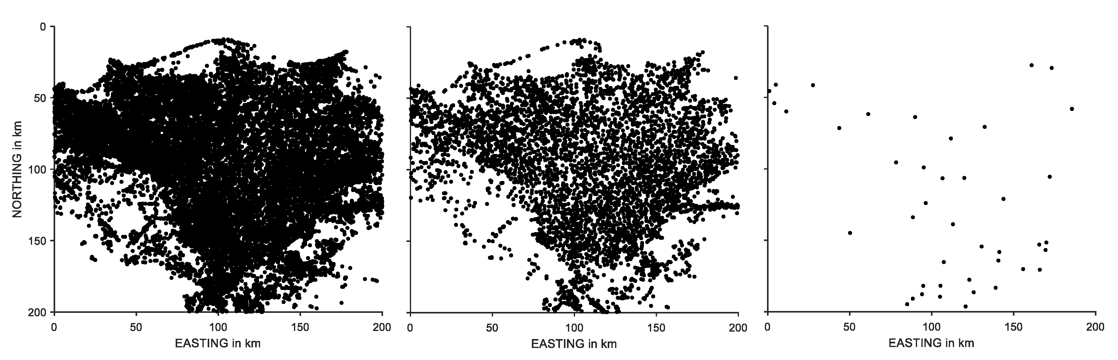
4.3. Classes

The small percentage of regular structures in Section 4.1 seems surprising when visually comparing the results to the GUF data, e.g., for Egypt (see Figure 4). The larger cities in the Nile Delta appear to be equidistant to each other, like it was shown for the cities in the Nile Valley [15]. Taking that into account a second analysis regarding only settlement objects larger in size, is carried out.
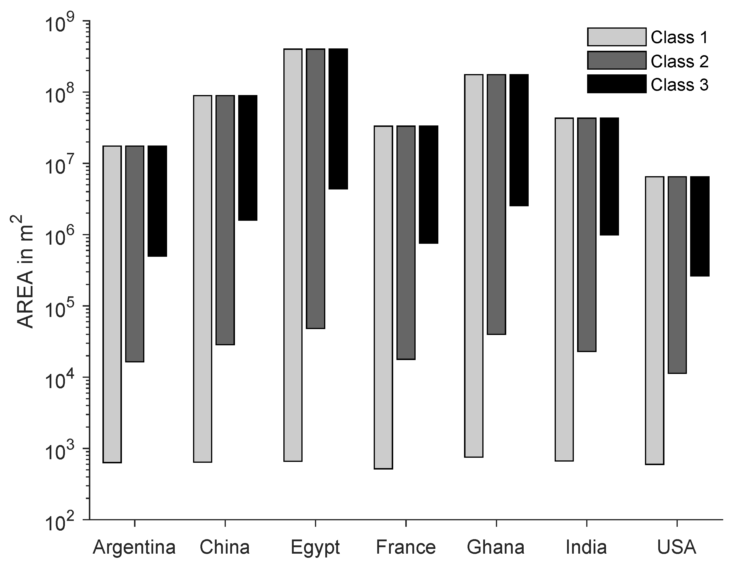
The data is divided into three logarithmic bins, ranging from the smallest object’s area to the largest object’s area. The entirety of objects, contained in the three bins, has been analysed in the previous subsections. In the following, this data set is referred to as Class 1. The middle and the last bin containing medium and large objects are denoted as Class 2, while the large objects are representing Class 3. For a visualisation of the data sets’ division into classes, please refer to Figure A1. The different classes in the data set Egypt are depicted in Figure 8.
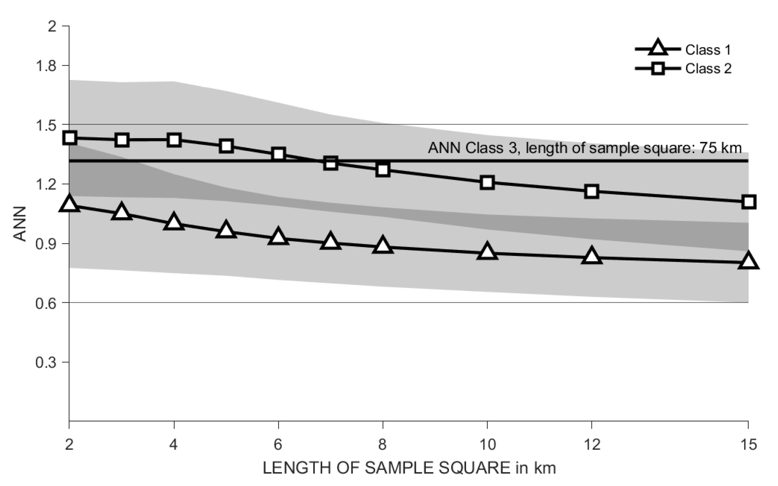
Repeating the described analysis with regarding only Class 2, the mean ANN in the data set Egypt increases, see Figure 9. In the data set Egypt there are only few objects in Class 3, that is why the sample square length must be increased significantly to allow a evaluation of the ANN . Therefore, the analysis results are not easily comparable with those for Class 1 and Class 2. To get an impression of the results for Class 3, Figure 9 gives the average ANN for sample squares with edge length equal to 75 km, taking into account only the objects of Class 3.
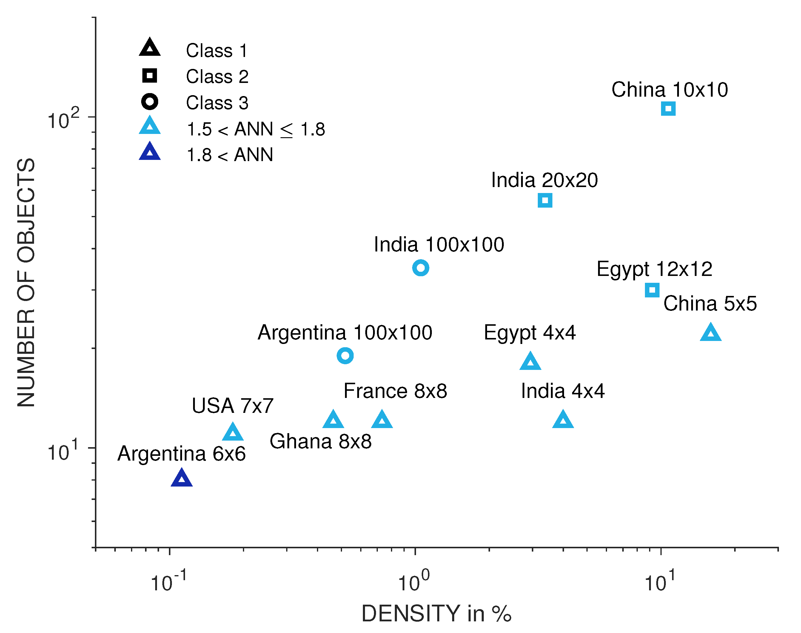
Similar results can be obtained by analysing Class 2 or Class 3 in the other data sets. Some data sets show higher proportions of regular windows in Class 3 than in Class 1, while others show higher proportions of regular windows in Class 2 than in Class 1. This leads to the hypothesis that settlement objects larger in size are arranged in a more regular pattern than the entirety of settlement objects.
When not just identifying the ANN in the sample squares but also the number of settlement objects regarded to calculate the index, it becomes clear that the sample squares with higher ANN usually include less objects (see Table A2). When analysing Class 2 and Class 3, the number of settlement objects decreases while the sample square’s edge length is kept constant. One may argue that the ANN in Class 2 and Class 3 therefore only increases because decreasing number objects in the sample squares. Regarding Table 2 this is not the case. Only for small sample squares with high ANN the data set Class 1 includes more data points than in Class 2. For larger sample squares the number of objects increases when moving from Class 1 to Class 2.

4.4. Regular Settlement Structures

None of the seven regions studied consists mainly of regular settlement structures. However, regular structures can be identified for all seven data sets—see Figure 10. Table 3 shows three such sections with ANN > 1.5 from the GUF and their parameters. It should be noted that the sections of the data sets China and Egypt for Class 2 do not appear to be distributed as regularly as the high ANN suggests. This is due to the fact that in Class 2 the small objects, which are, in this case, clustered around the larger ones, are not taken into account.

5. Discussion

The regions investigated in this study, especially rural areas, show different settlement patterns. The GUF is analysed with three parameters (number, density and regularity) that define a two dimensional pattern without considering the shape of the different objects. However, the analysis carried out is limited to a specific data set at a defined point in time. When assessing the results, it must be taken into account that the data may contain artefacts that are not discussed further here. For an evaluation of the original GUF data, please refer to the corresponding publications [37].
Looking at the size distribution of the different settlements and their mean value, it is striking that the values of ~0.01 km 2 found here are similar to those from intra-urban analyses [35,36]. This size seems to be an universal quantity of settlement structures, as it is also similar to the size of city blocks in American and Australian Cities [38].
We use the ANN as a method to quantify the regularities of patterns in awareness of the limitations of this approach: The influences of the area and number of objects taken into account for the calculation cannot be neglected (for a more detailed discussion on pattern indices we refer to the work in [39]). The disadvantages are understandable, as the spatial arrangement of a structure is reduced to a single parameter leading to an information loss. As the A N N still gives a first indication of the regularity of the pattern, it is an appropriate metric to answer the research questions formulated above.
Looking at the analysed regions from a macroscopic view, settlement clusters can be found, especially towards the coastlines. This is due to the fact that the process of settlement formation does not take place homogeneously over an area, but the proximity to resources and infrastructure (fishing, trade and economy) seems to play a role in the choice of location. The area boundaries also have a great influence on the result: while south of the region studied in Ghana the Atlantic Ocean begins directly and north of it the rainforest, in China the region is part of a very large inter-urban structure with high regularities [16].
The empirical results show a correlation between high density and a high number of objects (Table A2). At the same time, the density and the number of objects correlate strongly ( R = 0.9327 ) with the percentage of areas of high regularity (high A N N ), especially when using small investigation windows (2 × 2 km 2 ). With larger windows, the number of objects in areas with high A N N values decreases, so that it is uncertain how valid the results on the regularity are. It is also qualitatively shown in Table 3 that although density and ANN can be mapped, the size distribution in the empirical data fluctuates more than a theoretically regular pattern. As indicated by an analysis for large cities in the Nile Valley [15], the analyses can be continued in different classes. In further studies, the regularity of the larger cities introduced in Section 4.3 should be examined in detail.
At the beginning of this paper we asked the question whether urban structures (or parts of them) are arranged in a regular pattern and thus exhibit a typical property of non-equilibrium pattern formation in dissipative, open systems. As one might expect, regular structures cannot be observed in the entire study areas. However, we have been able to identify regular settlement patterns, especially in areas with a high number and density of settlement structures.
Based on these findings, a further step is to investigate which models can be used to depict the pattern formation of urban structures. For example, it can be analysed whether reaction–diffusion models, the pattern formation through the interaction of different morphogenes, are suitable to describe the structure formation. For this purpose, fundamental work by Rudy et al. [40] or Zhao et al. [41] can be referred to, who have identified the underlying mechanisms of pattern formation by analysing image sequences. Their proposed methods can be used to analyse time-resolved settlement maps and quantify their changes by using concepts from physics.
Since regular structures were identified mainly in small evaluation windows, the nonlinear pattern formation models to be developed should also focus primarily on small scales.

6. Conclusions

The results in this paper aid to answer whether settlements are arranged regularly in different regions of the world. The motivation for posing this question is whether cities as thermodynamic open systems share similarities in pattern with dissipative structures.
The settlement patterns of seven regions in five continents were investigated. While the region in China had a high number of settlement objects and a high settlement density, and the regions in the USA and Argentina had a low number of objects and settlement density, the other regions studied (Ghana, France, India and Egypt) were in between. The settlement density and the number of settlements correlate with each other, which can be explained by the relatively similar size distributions of the settlements with a geometric mean of nearly 0.01 km 2 . The number of settlements as well as the density correlates with the proportion of sample windows with a high regularity A N N > 1.5 . The analyses with the highest resolution (sample window of 2 × 2 km 2 ) showed that between approximately 1% (USA) and 14% (China) of the investigated area show regular settlement structures. This means that the more densely populated a region is, the more likely it is that regular settlement structures can be found in it.
These results can be used to develop mathematical models that can describe the pattern formation of urban structures by models of non-equilibrium thermodynamics. Furthermore, the results could be expanded in future work and brought together with other research fields: For example, (i) in infrastructural studies it could be analysed whether the temporal development of transport infrastructures had an influence on the inter-urban pattern formation. Furthermore, (ii) it could be investigated to what extent political systems (politics and policies) are correlated with pattern formation. These aspects could then be explicitly considered in the mathematical models. Finally, (iii) it can be investigated to what extent the economic development of a region is related to or influences the arrangement of settlements. All these insights are useful for a better understanding of urbanisation processes and can, for example, help urban planners to develop sustainable concepts to meet these challenges.

Author Contributions

Conceptualisation, John Friesen and Jakob Hartig; Methodology, Katharina Henn, John Friesen and Jakob Hartig; Formal analysis, Katharina Henn; Investigation, Katharina Henn; Writing—original draft preparation, Katharina Henn, John Friesen and Jakob Hartig; Writing—review and editing, Katharina Henn, John Friesen and Jakob Hartig; Visualisation, Katharina Henn; Supervision, Peter F. Pelz; Project administration, Peter F. Pelz. All authors have read and agreed to the published version of the manuscript.

Funding

This research received no external funding.

Acknowledgments

We thank the German Aerospace Center for providing the data of the Global Urban Footprint and acknowledge support by the DFG and the Open Access Publishing Fund of Technical University of Darmstadt for publishing.

Conflicts of Interest

The authors declare no conflict of interest.

Abbreviations

The following abbreviations are used in this manuscript.
ANN Average-Nearest Neighbour Index
CPTcentral place theory
DLRGerman Aerospace Center
GUFGlobal Urban Footprint
s.s.sample square

Appendix A. Further Data

Table A1. Coordinates of all seven considered datasets. The reference system is WGS 84, the coordinates are given in decimal degrees.
Data SetWestSouthEastNorth
Argentina−63.424−33.800−61.265−31.996
China114.06532.800116.20034.603
Egypt30.01429.87632.08431.680
France3.35047.4016.00049.200
Ghana−2.2785.4190.4737.228
India74.40028.89676.45130.700
USA−100.00038.50097.70740.301
Figure A1. The columns represent the range of the settlement objects’ area for the different classes in each data set.
Ijgi 09 00541 g0a1
Table A2. Percentage of sample squares (s.s.) with ANN > 1.5 for each data set and the according number of data points N considered to evaluate the ANN > 1.5 in these s.s. Additionally, the percentage of sample squares with ANN > 1.5 and z < 2.58 or z > 2.58 , and the average number of objects N in these sample squares.
2 km4 km6 km8 km10 km12 km15 km
Argentina
% of s.s. with ANN > 1.5 4.287.455.052.691.250.940.23
% of s.s. with ANN > 1.5 and z < 2.58 or z > 2.58 68.1871.5379.4285.0381.6387.5075.00
average N in s.s. with ANN > 1.5 5.445.696.777.207.107.656.20
average N in s.s. with ANN > 1.5 and z < 2.58 or z > 2.58 5.585.857.167.497.498.006.33
China
% of s.s. with ANN > 1.5 13.971.750.070.000.000.000.00
% of s.s. with ANN > 1.5 and z < 2.58 or z > 2.58 82.9694.71100.000.000.000.000.00
average N in s.s. with ANN > 1.5 6.5612.2422.86----
average N in s.s. with ANN > 1.5 and z < 2.58 or z > 2.58 6.7912.6022.86----
Egypt
% of s.s. with ANN > 1.5 9.582.300.500.180.160.000.03
% of s.s. with ANN > 1.5 and z < 2.58 or z > 2.58 77.0384.7375.7676.9258.330.00100.00
average N in s.s. with ANN > 1.5 6.087.546.427.316.75-10
average N in s.s. with ANN > 1.5 and z < 2.58 or z > 2.58 6.317.916.688.007.57-10
France
% of s.s. with ANN > 1.5 1.870.950.310.070.000.000.00
% of s.s. with ANN > 1.5 and z < 2.58 or z > 2.58 70.671.4367.8671.430.000.000.00
average N in s.s. with ANN > 1.5 5.785.895.867.14---
average N in s.s. with ANN > 1.5 and z < 2.58 or z > 2.58 6.006.096.167.60---
Ghana
% of s.s. with ANN > 1.5 1.622.862.030.870.280.060.19
% of s.s. with ANN > 1.5 and z < 2.58 or z > 2.58 74.8070.8379.2882.5486.36100.0068.75
average N in s.s. with ANN > 1.5 6.315.536.687.248.955.805.63
average N in s.s. with ANN > 1.5 and z < 2.58 or z > 2.58 6.625.616.977.529.425.805.64
India
% of s.s. with ANN > 1.5 7.304.001.560.650.310.200.08
% of s.s. with ANN > 1.5 and z < 2.58 or z > 2.58 70.2775.2376.7467.8085.7194.44100.00
average N in s.s. with ANN > 1.5 5.826.346.306.596.327.3911.29
average N in s.s. with ANN > 1.5 and z < 2.58 or z > 2.58 6.036.696.547.236.547.4111.29
USA
% of s.s. with ANN > 1.5 0.802.733.512.601.730.800.21
% of s.s. with ANN > 1.5 and z < 2.58 or z > 2.58 63.6458.5477.3073.9976.4385.5194.44
average N in s.s. with ANN > 1.5 5.675.375.916.096.416.867.28
average N in s.s. with ANN > 1.5 and z < 2.58 or z > 2.58 5.865.426.096.326.727.057.41

References

  1. Retief, F.; Bond, A.; Pope, J.; Morrison-Saunders, A.; King, N. Global megatrends and their implications for environmental assessment practice. Environ. Impact Assess. Rev. 2016, 61, 52–60. [Google Scholar] [CrossRef]
  2. Zhu, Z.; Zhou, Y.; Seto, K.C.; Stokes, E.C.; Deng, C.; Pickett, S.T.; Taubenböck, H. Understanding an urbanizing planet: Strategic directions for remote sensing. Remote. Sens. Environ. 2019, 228, 164–182. [Google Scholar] [CrossRef]
  3. Batty, M. The New Science of Cities; MIT Press: Cambridge, MA, USA, 2013. [Google Scholar]
  4. Batty, M. Building a science of cities. Cities 2012, 29, S9–S16. [Google Scholar] [CrossRef] [Green Version]
  5. Portugali, J. Complexity, Cognition and the City; Springer complexity, Springer: Berlin/Heidelberg, Germany; New York, NY, USA, 2011. [Google Scholar]
  6. Taubenbock, H.; Debray, H.; Qiu, C.; Schmitt, M.; Wang, Y.; Zhu, X. Seven city types representing morphologic configurations of cities across the globe. Cities 2020, 105, 102814. [Google Scholar] [CrossRef]
  7. Benenson, I.; Torrens, P.M. Geosimulation: Automata-Based Modelling of Urban Phenomena; John Wiley & Sons: Hoboken, NJ, USA, 2004. [Google Scholar]
  8. Liu, Y.; Batty, M.; Wang, S.; Corcoran, J. Modelling urban change with cellular automata: Contemporary issues and future research directions. Prog. Hum. Geogr. 2019. [Google Scholar] [CrossRef]
  9. Rathore, M.M.; Ahmad, A.; Paul, A.; Rho, S. Urban planning and building smart cities based on the internet of things using big data analytics. Comput. Netw. 2016, 101, 63–80. [Google Scholar] [CrossRef]
  10. Wu, N.; Silva, E.A. Artificial intelligence solutions for urban land dynamics: A review. J. Plan. Lit. 2010, 24, 246–265. [Google Scholar]
  11. Zhao, K.; Tarkoma, S.; Liu, S.; Vo, H. Urban human mobility data mining: An overview. In Proceedings of the 2016 IEEE International Conference on Big Data (Big Data), Washington, DC, USA, 5–8 December 2016; IEEE: Piscataway, NJ, USA, 2016; pp. 1911–1920. [Google Scholar]
  12. Healy, K. Fuck Nuance. Sociol. Theory 2017, 35, 118–127. [Google Scholar] [CrossRef]
  13. Christaller, W. Die Zentralen Orte in Süddeutschland: Eine Ökonomisch-Geographische Untersuchung Über die Gesetzmässigkeit der Verbreitung und Entwicklung der Siedlungen mit Städtischen Funktionen; Wissenschaftliche Buchgesellschaft: Darmstadt, Germany, 1933. [Google Scholar]
  14. Allen, P.M.; Sanglier, M. A dynamic model of growth in a central place system. Geogr. Anal. 1979, 11, 256–272. [Google Scholar] [CrossRef]
  15. AbouKorin, A.A. Spatial analysis of the urban system in the Nile Valley of Egypt. Ain Shams Eng. J. 2018, 9, 1819–1829. [Google Scholar] [CrossRef]
  16. Yang, R.; Xu, Q.; Long, H. Spatial distribution characteristics and optimized reconstruction analysis of China’s rural settlements during the process of rapid urbanisation. J. Rural Stud. 2016, 47, 413–424. [Google Scholar] [CrossRef]
  17. Krugman, P. The Self-Organizing Economy; Number 338.9 KRU 1996; CIMMYT: Mexico City, Mexico, 1996. [Google Scholar]
  18. Cross, M.C.; Hohenberg, P.C. Pattern formation outside of equilibrium. Rev. Mod. Phys. 1993, 65, 851. [Google Scholar] [CrossRef] [Green Version]
  19. Purvis, B.; Mao, Y.; Robinson, D. Entropy and its application to urban systems. Entropy 2019, 21, 56. [Google Scholar] [CrossRef] [Green Version]
  20. Levashova, N.; Sidorova, A.; Semina, A.; Ni, M. A Spatio-Temporal Autowave Model of Shanghai Territory Development. Sustainability 2019, 11, 3658. [Google Scholar] [CrossRef] [Green Version]
  21. Medda, F.; Nijkamp, P.; Rietveld, P. A Morphogenetic Perspective on Spatial Complexity. In Complexity and Spatial Networks; Reggiani, A., Nijkamp, P., Eds.; Springer: Berlin/ Heidelberg, Germany, 2009; pp. 51–60. [Google Scholar]
  22. Pelz, P.F.; Friesen, J.; Hartig, J. Similar size of slums caused by a Turing instability of migration behavior. Phys. Rev. 2019, 99. [Google Scholar] [CrossRef] [Green Version]
  23. Barrington-Leigh, C.; Millard-Ball, A. A century of sprawl in the United States. Proc. Natl. Acad. Sci. USA 2015, 112, 8244–8249. [Google Scholar] [CrossRef] [Green Version]
  24. Urbieta, P.; Fernandez, E.; Ramos, L.; Méndez Martínez, G.; Bento, R. A land-cover based urban dispersion indicator suitable for highly dispersed, discontinuously artificialized territories: The case of continental Portugal. Land Use Policy 2019, 85, 92–103. [Google Scholar] [CrossRef] [Green Version]
  25. Romano, B.; Zullo, F.; Fiorini, L.; Ciabò, S.; Marucci, A. Sprinkling: An Approach to Describe Urbanization Dynamics in Italy. Sustainability 2017, 9, 97. [Google Scholar] [CrossRef] [Green Version]
  26. Saganeiti, L.; Favale, A.; Pilogallo, A.; Scorza, F.; Murgante, B. Assessing Urban Fragmentation at Regional Scale Using Sprinkling Indexes. Sustainability 2018, 10, 3274. [Google Scholar] [CrossRef] [Green Version]
  27. Ewing, R.H. Characteristics, Causes, and Effects of Sprawl: A Literature Review. In Urban Ecology: An International Perspective on the Interaction Between Humans and Nature; Marzluff, J.M., Shulenberger, E., Endlicher, W., Alberti, M., Bradley, G., Ryan, C., Simon, U., ZumBrunnen, C., Eds.; Springer: Boston, MA, USA, 2008; pp. 519–535. [Google Scholar]
  28. Kondo, S.; Miura, T. Reaction-diffusion model as a framework for understanding biological pattern formation. Science 2010, 329, 1616–1620. [Google Scholar] [CrossRef] [Green Version]
  29. Esch, T.; Heldens, W.; Hirner, A.; Keil, M.; Marconcini, M.; Roth, A.; Zeidler, J.; Dech, S.; Strano, E. Breaking new ground in mapping human settlements from space—The Global Urban Footprint. Isprs J. Photogramm. Remote. Sens. 2017, 134, 30–42. [Google Scholar] [CrossRef] [Green Version]
  30. Esch, T.; Bachofer, F.; Heldens, W.; Hirner, A.; Marconcini, M.; Palacios-Lopez, D.; Roth, A.; Üreyen, S.; Zeidler, J.; Dech, S.; et al. Where we live—A summary of the achievements and planned evolution of the global urban footprint. Remote Sens. 2018, 10, 895. [Google Scholar] [CrossRef] [Green Version]
  31. Esch, T.; Schenk, A.; Ullmann, T.; Thiel, M.; Roth, A.; Dech, S. Characterization of land cover types in TerraSAR-X images by combined analysis of speckle statistics and intensity information. IEEE Trans. Geosci. Remote. Sens. 2011, 49, 1911–1925. [Google Scholar] [CrossRef]
  32. Hudson, J.C. A Location Theory for Rural Settlement. Ann. Assoc. Am. Geogr. 1969, 59, 365–381. [Google Scholar] [CrossRef]
  33. Friesen, J.; Hartig, J.; Henn, K.; Pelz, P.F. Diffusion-driven demographics—Turing model as a concept for the emergence of sedentism. arXiv 2020, arXiv:2005.05107. [Google Scholar]
  34. Clark, J.P.; Evans, C.F. Distance to Nearest Neighbor as a Measure of Spatial Relationships in Populations. Ecology 1954, 35, 445–453. [Google Scholar] [CrossRef]
  35. Friesen, J.; Taubenböck, H.; Wurm, M.; Pelz, P.F. The similar size of slums. Habitat Int. 2018, 73, 79–88. [Google Scholar] [CrossRef]
  36. Friesen, J.; Taubenböck, H.; Wurm, M.; Pelz, P.F. Size distributions of slums across the globe using different data and classification methods. Eur. J. Remote Sens. 2019, 52, 99–111. [Google Scholar] [CrossRef] [Green Version]
  37. Klotz, M.; Kemper, T.; Geiß, C.; Esch, T.; Taubenböck, H. How good is the map? A multi-scale cross-comparison framework for global settlement layers: Evidence from Central Europe. Remote Sens. Environ. 2016, 178, 191–212. [Google Scholar] [CrossRef] [Green Version]
  38. Siksna, A. The effects of block size and form in North American and Australian city centres. Urban Morphol. 1997, 1, 19–33. [Google Scholar]
  39. Goodall, D.W.; West, N.E. A comparison of techniques for assessing dispersion patterns. Vegetatio 1979, 40, 15–27. [Google Scholar] [CrossRef]
  40. Rudy, S.H.; Brunton, S.L.; Proctor, J.L.; Kutz, J.N. Data-driven discovery of partial differential equations. Sci. Adv. 2017, 3, e1602614. [Google Scholar] [CrossRef] [PubMed] [Green Version]
  41. Zhao, H.; Storey, B.D.; Braatz, R.D.; Bazant, M.Z. Learning the physics of pattern formation from images. Phys. Rev. Lett. 2020, 124, 060201. [Google Scholar] [CrossRef] [PubMed]
Figure 1. Types of pattern classified by number of objects, density and regularity.
Ijgi 09 00541 g001
Figure 2. Workflow of this paper starting from the empirical data of the Global Urban Footprint (GUF), a binary settlement map derived from satellite data (Section 3.1) [29,30]. Preprocessing of the data as follows (Section 3.2) by identifying related objects and determine their centre of gravity and analysis of the spatial distribution of the number of objects, density and regularity (Section 4).
Ijgi 09 00541 g002
Figure 3. Schematic geographical position of the seven analysed areas in Argentina, Egypt, China, France, Ghana, India and USA.
Ijgi 09 00541 g003
Figure 4. Parts of the Global Urban Footprint (GUF). The data set Egypt includes the Nile Delta (left), the investigated region in China is located in den province Henan and Anhui (right).
Ijgi 09 00541 g004
Figure 5. Number of objects, density and ANN for sliding window analysis for windows of sample size of 8 km.
Ijgi 09 00541 g005
Figure 6. Results for the mean ANN calculated in sample squares of different edge length in all data sets. The grey area represents the standard deviation of the calculated values.
Ijgi 09 00541 g006
Figure 7. Box plot showing the size distribution of settlement objects in all seven data sets. The arithmetic mean is marked with a red star for each data set.
Ijgi 09 00541 g007
Figure 8. Data points for Class 1, Class 2, Class 3 (from left to right).
Ijgi 09 00541 g008
Figure 9. Average ANN in sample squares of different length for Class 1 and Class 2 in the data set Egypt.
Ijgi 09 00541 g009
Figure 10. The marker represent the parameters of the chosen sample squares. The numbers following the data set’s name indicate the edge length of the sample square.
Ijgi 09 00541 g010
Table 1. Table containing the number N 0 of objects in every data set, and the geometric mean S 0 of the objects’ area. The data sets’ average characteristic size is S ¯ 0 = 0.0112 ± 0.0051  km 2 . All values are defined as in [35].
Data Set N 0 S 0 in m 2 σ l = S 0 in mDensity in %
Argentina711949951.204570.70.59
China65,73619,1791.6694138.511.4
Egypt22,74413,5121.6810116.25.94
France20,77176211.667087.32.15
Ghana914714,2931.5846119.61.91
India17,27014,2661.7161119.43.63
USA660544711.279266.90.28
Table 2. For Class 1 and Class 2 in the data set Egypt, percentage of sample squares (s.s.) with ANN > 1.5 are listed; N is the average number of data points in these sample squares.
s.s. Length 3 km5 km7 km10 km12 km15 km
Class 1% of sample squares5.770.730.310.160.000.03
N6.797.897.006.75-10.00
Class 2% of sample squares38.9135.2620.206.432.600.65
N5.416.519.4416.0920.0815.34
Table 3. Examples for regular settlement structures in the data sets China and Egypt.
CHINA Class 1CHINA Class 2EGYPT Class 3
s.s. Length5 km10 km12 km
parameters
N2210630
ϱ in %15.9510.729.21
ANN 1.691.501.57
z6.229.875.98
original GUF data Ijgi 09 00541 i001 Ijgi 09 00541 i002 Ijgi 09 00541 i003

