Drift Invariant Metric Quality Control of Construction Sites Using BIM and Point Cloud Data

Abstract

Construction site monitoring is currently performed through visual inspections and costly selective measurements. Due to the small overhead in construction projects, additional resources are scarce to frequently conduct a metric quality assessment of the constructed objects. However, contradictory, construction projects are characterised by high failure costs which are often caused by erroneously constructed structural objects. With the upcoming use of periodic remote sensing during the different phases of the building process, new possibilities arise to advance from a selective quality analysis to an in-depth assessment of the full construction site. In this work, a novel methodology is presented to rapidly evaluate a large number of built objects on a construction site. Given a point cloud and a set of as-design BIM elements, our method evaluates the deviations between both datasets and computes the positioning errors of each object. Unlike the current state of the art, our method computes the error vectors regardless of drift, noise, clutter and (geo)referencing errors, leading to a better detection rate. The main contributions are the efficient matching of both datasets, the drift invariant metric evaluation and the intuitive visualisation of the results. The proposed analysis facilitates the identification of construction errors early on in the process, hence significantly lowering the failure costs. The application is embedded in native BIM software and visualises the objects by a simple color code, providing an intuitive indicator for the positioning accuracy of the built objects.

1. Introduction

Failure costs are prevalent in the construction industry and range from 5% to 20% of the total project cost [1,2]. Furthermore, most of the error-induced costs occur during the construction of the building’s structural elements. In the work of Love et al. [3], it is stated that non-conformances during structural steel and concrete works constitute a total of over 50% of the failure costs. It is therefore vital to asses the quality of constructed elements during the execution phase. This includes the evaluation of the constructed elements with respect to their as-design shape in terms of geometry and appearance [4]. In this work, the emphasis is on the metric quality assessment and more specifically on the positioning errors of the objects. The resulting information can also be used for progress monitoring and for quantity take-offs [5]. Overall, the early detection of erroneously placed objects results in a strong cutback in the related repair costs, hence decreasing the overall failure costs of the project.

Despite its importance, the automation of construction site and progress monitoring workflows is lacking [6,7]. The construction industry currently still relies on visual inspections and sparse selective measurements executed by workers on site such as foremen and construction site managers. However, for an accurate and correct assessment of the positioning quality, these methods do not suffice. Alternatively, costly surveyor teams are employed to inspect the objects but due to budget limitations, only a small subset of the objects is evaluated. As a result, construction errors are not detected in time and cause the above described failure costs.

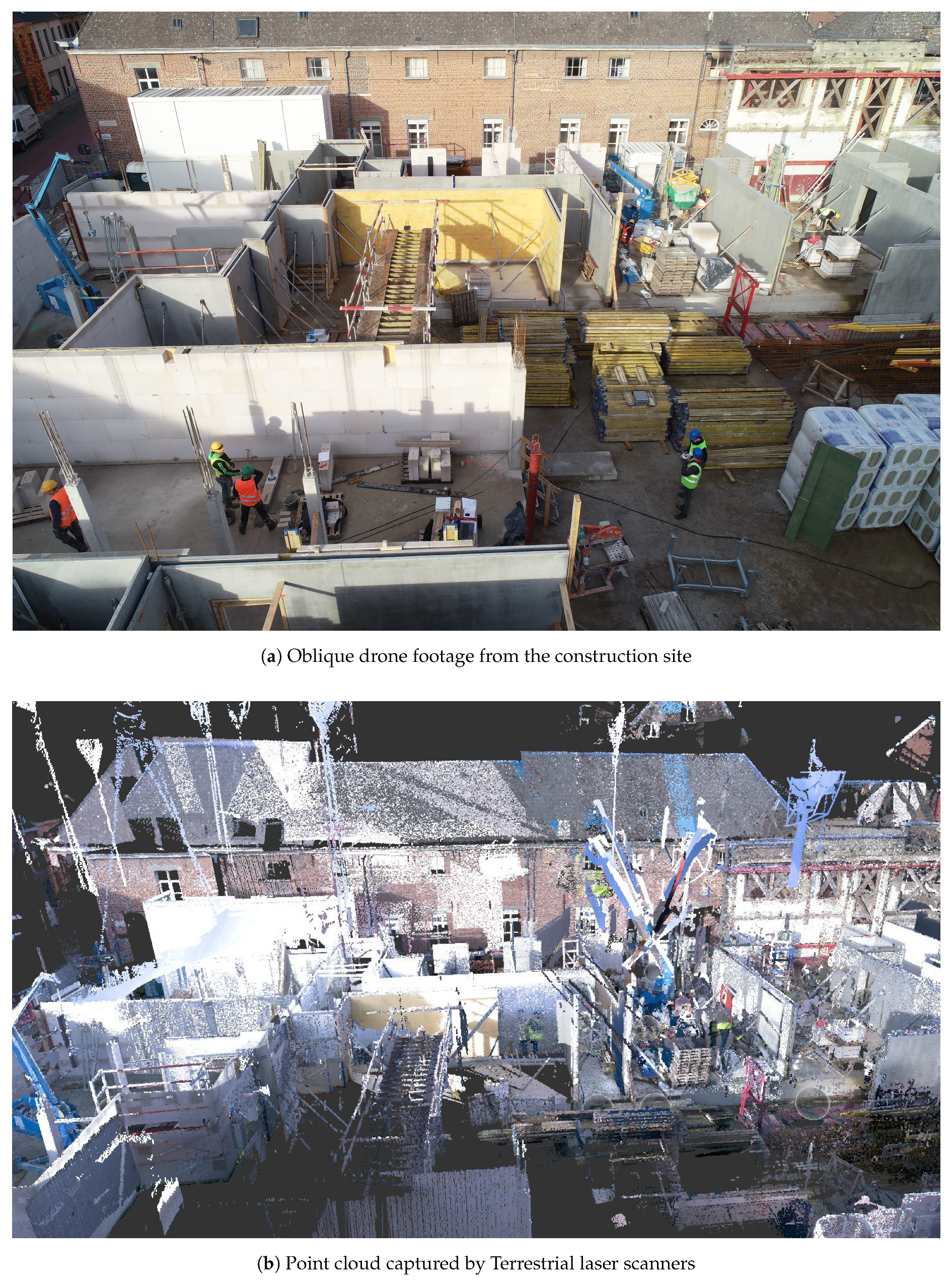
One approach to systematically evaluate construction sites is through point cloud data produced by remote sensing that is, laser scanning or photogrammetry, which produce vast amounts of geometric and visual information of the construction site in a more cost-effective manner (Figure 1). For progress monitoring purposes and metric quality assessments, it is paramount that these recorded datasets are properly (geo)referenced [8]. Traditionally, the procedure to align a point cloud with the corresponding as-design BIM model relies on a rigid body transformation of the former based on geometric correspondences [9]. Although this is a common practice, significant erroneous results may be encountered as inaccuracies still persist in the point cloud data. One of the driving factors is sensor drift, caused by propagating registration errors [10]. Especially for larger construction sites with complex layouts, clutter and poor accessibility, significant drift effects can be expected. Moreover, the measurement noise generated on construction site objects is substantial which further complicates the registration [11]. The presence of clutter and construction materials also inevitably result in (partial) occlusions of numerous construction elements [12]. This complicates their assessment, as analyses can only be executed on the visible parts of the elements.

In this research, we propose a novel method to assess the metric quality of building elements regardless of drift, noise, partial occlusions and suboptimal (geo)referencing. More specifically, we compute the systematic positioning error of each built object on a construction site given its as-design shape and neighboring objects. The framework we present aids the construction industry to assess construction site objects more profoundly in an efficient way and at a reduced cost (Figure 1). In summary, the main contributions are:

• A robust framework to assess the metric quality of a large number of construction site objects in an efficient manner
• A novel method that evaluates the discrepancies between a recorded point cloud and the BIM objects considering frequent construction site obstacles
• An intuitive visualization displaying objects according to the Level of Accuracy (LOA) specification ranges

The remainder of this work is structured as follows. In Section 2, the related work on metric quality assessment is discussed. This is followed by Section 3, which gives an overview of our method and its most important contributions and advantages. In Section 4 the methodology of our application is presented. The results of the application are presented and discussed in Section 5 and Section 6. Finally, the conclusions and future optimisations are presented in Section 7.

2. Background & Related Work

Construction site assessment is a vital aspect of a project’s execution phase. Nevertheless, the automation of this procedure is still very much the topic of ongoing research [13,14]. An exhaustive literature overview of construction monitoring is presented by Alizadehsalehi et al. [15]. In this section, we discuss the works that focus on remote sensing data capture and those related to metric quality assessment on site.

2.1. Construction Site Geometry

The capture of construction sites is problematic. There is a plethora of techniques, both static and mobile, that can capture a construction site environment [16,17,18,19]. However, several inherent problems yet remain. A first obstacle is the site complexity with its limited accessibility due to construction operations and the presence of building materials, equipment, workers and support structures such as moldings. As a result, the point cloud data is heavily occluded and more drift can accumulate due to suboptimal sensor positioning and reduced fields of view [20,21]. Kalyan et al. [22] report that while construction sites can be captured, the resulting point cloud often lacks the accuracy to check for building tolerances. Zhang et al. [23] recognise this issue and propose an occlusion evaluation during the data acquisition. However, the registration of the datasets is also complicated by the objects themselves. The lack of texture for photogrammetric processes and the lack of geometric data dispersion for lidar approaches cause errors in the registration procedures of both approaches. As a result, the registration errors of mobile sensors or photogrammetric processes can easily reach up to several centimeters in average sized construction sites [10].

A second obstacle is the 3D point accuracy influenced by noise, drift and (geo)referencing. Most quality assessments rely on an accurate registration between the as-design model and the observed construction site [15]. However, the (geo)referencing of a construction site environment is error prone due to occluded markers, the site complexity and GPS denied zones. As such, GPS (geo)referencing accuracy of photogrammetric and lidar processes again is several centimeters in average sized construction sites if costly surveyor teams are not employed [8]. Noise is also rampant in construction sites due to the operations that are accompanied by the presence of temporary objects, workers, dust, vibrations and so on. Additionally, construction materials such as rebar are prone to noise due to their reflectivity characteristics and shape. Overall, it is stated that the noise, clutter, drift and (geo)referencing errors along with the occlusions complicate the proper assessment of an object’s positioning errors and must be taken into consideration.

2.2. Metric Quality Assessment

The assessment of the metric quality of a completed construction site object involves the estimation of the positioning errors of the object with respect to the building tolerances [24]. It is often referred to as scan-vs.-BIM [9,25] and is considered a high accuracy task which is challenging due to above defined errors [26]. For this reason, the spatial component of the analysis is sometimes overlooked [27]. For instance, Tang et al. and Anil et al. [28,29] make an assessment by purely reasoning on the visual information of an object without considering its location. For those that do include the metrics, the most common way is to (geo)reference the dataset and compute the shortest Euclidean distances between the sampled point cloud and the ground truth. For instance, Liu et al. [30] evaluate the dimensional accuracy of structure components given a perfectly aligned point cloud. Similarly, Nguyen et al. [20] perform on-site dimensional inspections given a properly referenced point cloud.

There are a number of researchers that attempt to enhance the (geo)referencing accuracy by computing an additional transformation between both datasets. Schnabel et al. [31] apply RANSAC-based procedures [32] to match as-design shapes to the point cloud. However, they only reach an accuracy of circa 0.15 m in a cloud-to-cloud based approach, which is insufficient for thorough positioning assessments. To improve the their target-based registration, Maalek et al. [33] actively mitigate clutter by detecting planes in the point cloud and removing outliers from the dataset. Xu et al. [34] also retrieve geometric primitives from construction sites and show that robust matching can overcome construction site noise for both photogrammetric and lidar datasets. Also from a computer vision approach, several algorithms such as Oriented FAST and Rotated BRIEF b (ORB) [35] and Signature of Histograms of Orientations (SHOT) [36] provide a solution for matching 3D shapes. However, the different types of data that is, point clouds and BIM models, with significant levels of noise and occlusions in the former and an abstract representation of the latter, make it challenging to exploit these algorithms [27]. An interesting alternative is to use Iterative Closest Point (ICP)-based [37] algorithms to retrieve the deviations between both datasets. These algorithms have proven to successfully retrieve the proper transformation between already closely aligned datasets such is the case with coarsely (geo)referenced construction site datasets [7,25,38,39,40]. The common concept of all aforementioned algorithms is that they consider the datasets as rigid bodies. Consequentially, the positioning errors are systematically exaggerated as these methods do not account for sensor noise and registration errors.

Closely related to quality control is damage inspection. This task has both the detection of progress monitoring and the assessment of the metric quality control. For instance, Valenca et al. [41] detect and assess cracks on concrete bridges using image processing supported by laser scanning survey. Similar to the evaluation of positioning errors, the proposed approaches assume a perfect alignment between the as-design objects and the observed data. Cabaleiro et al. [42], Zhong et al. [43], Adhikari et al. [44] all propose crack detection algorithms that build upon this assumption. It is interesting to note that this assumption does in fact hold up in smaller datasets where drift errors are less rampant.

Another closely related application to positioning errors is the dimensional evaluation of individual elements. This is also typically expressed as the shortest Euclidean distances between the sampled observations and the as-design shape of the objects [45,46]. However, several works also evaluate the translations and rotations of parts of the constructed elements such as presented by Wang et al. [47]. Dimension evaluations also include the association of the observed data with the parametric information that defines the object such as the radius of a pipe [7,9,48] or tunnel [49]. These methods show that the percentage and distribution of the observed surface of the object is a key factor in the reliability of the evaluation and needs to be taken into consideration. The reversed operation, that is, scan-to-BIM, such as presented by Tran et al. [50] also requires quality control but of the modeled objects. In these applications, exact positioning is always used since the measured point clouds are always assumed to be correct [51].

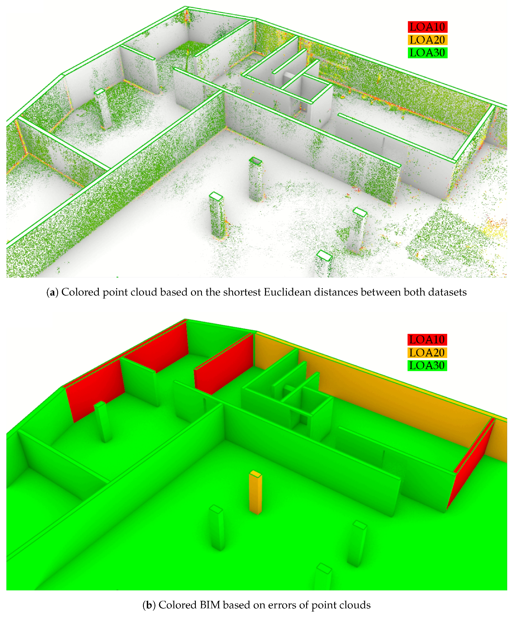
Given the transformations or deviations between the datasets, the results are communicated to the stakeholders. In it simplest form, this is a point cloud colored based on the deviations and a table showing the deviation parameters [20,29] (Figure 2a). Aside from the above discussed errors, the visualisation is heavily cluttered with stray points and noise which is challenging to evaluate by a user. Additionally, only the errors of the observed points are shown while stakeholders are interested in the positioning error of the entire object. As such, there is a mismatch between this representation and the expectations of the stakeholders. Similar to this study, Anil et al. [29] color the BIM instead of the point cloud. Each element is colored in a single color conform accuracy intervals, providing much needed clarity but also making it impossible to assess sub-element deviations. A popular set of accuracy intervals are the level of Accuracy (LOA) specification ranges which specify the measured and represented accuracy in a $95\%$ error interval [52]. The most commonly used intervals for construction tolerances are LOA30 $\left[\right|{\widehat{e}}_{w_i}|\le$ 0.0015 m] (green), LOA20 [0.0015 m $\le |{\widehat{e}}_{w_i}|\le$ 0.05 m] (orange) and LOA10 $\left[\right|{\widehat{e}}_{w_i}|\ge$ 0.05 m] (red). Alternatively, Chen and Cho [27] chose to represent both, which is resource intensive. Tabular representations are also considered to show the deviations such as presented in Wang et al. [53], Kalyan et al. [22] and Guo et al. [48]. However, the errors are still mainly reported for only the point cloud instead of the BIM.

3. Overview

In this section, a general overview of the pipeline is presented.

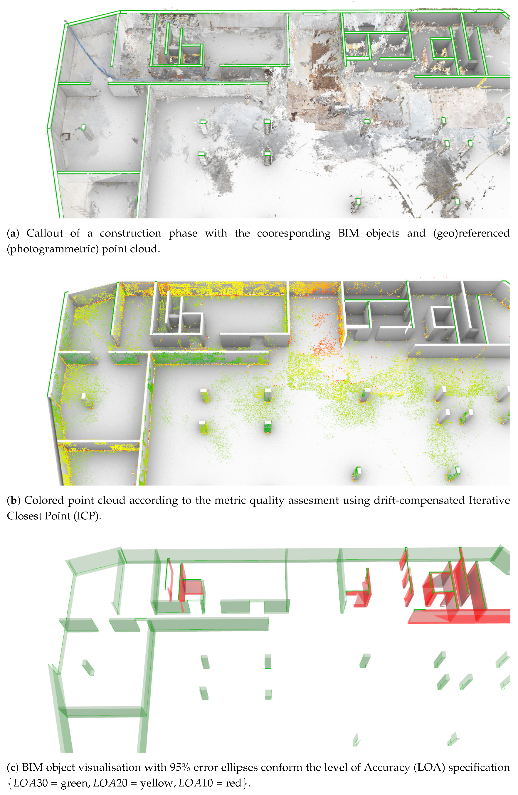
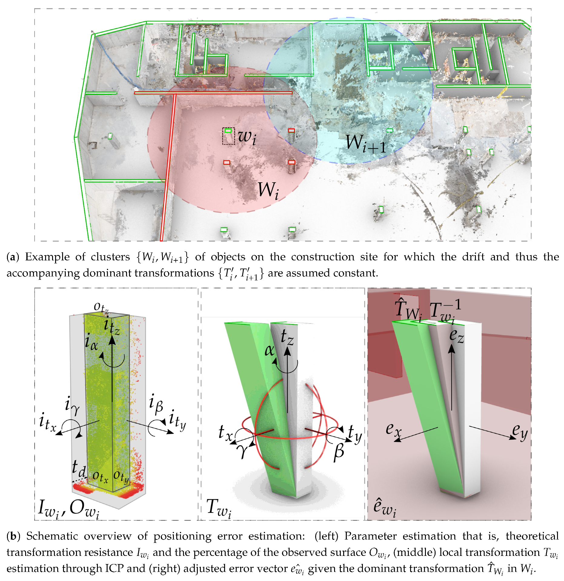
• The pipeline has two inputs, that is, a BIM model and a (geo)referenced point cloud (Figure 3a). In order for the method to properly operate, the majority of constructed elements should be built within tolerances and a minimum portion of the surface area of each target object should be observed in the point cloud. Also, the (geo)referencing accuracy of the point cloud should be equal or better than half of the average width of the target objects on the construction site.
• Prior to the metric quality assessment, the data is preprocessed. For every target object in the BIM, a mesh representation is generated and the (geo)referenced point cloud is segmented using these objects. Following, several object characteristics are computed including the theoretical transformation resistance and the percentage of the observed surface of the object, both of which are used to enhance the error assessment.
• The first step in the error assessment is the individual error estimation. An ICP-based algorithm is applied to compute the best fit transformation between an object’s as-design shape and its observed points. Given an object’s rotation and translation parameters, the $95\%$ error vector is established for the object. However, this error is exaggerated due to drift and (geo)referencing errors and thus should be compensated.
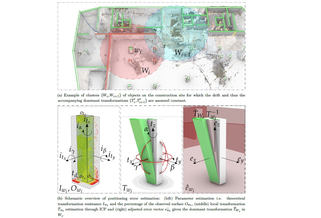
• The second step in the error assessment is the adjustment of each object’s error vector using the dominant transformation in the vicinity of that object (Figure 3b). To this end, a cost function is defined between every object and its nearest neighbors. Given each object’s characteristics and ICP error, the best fit parameters for the dominant transformation are defined. The adjusted positioning error vector is then established by applying both the individual and the dominant transformation.
• The resulting error vectors are used to visualise each object’s position errors. The error vectors are assigned to one of the Level of Accuracy (LOA) specification ranges and each BIM object is colored conform its respective interval (Figure 3c). The result is a colored BIM model and tabular error ellipses along the cardinal axes which can be intuitively interpreted by the stakeholders.

The final section of the methodology includes the implementation of the method. The method is tested on a simulated construction site with known ground truth and compared to a traditional metric quality assessment. Following, the method is also applied to a photogrammetric and lidar dataset to evaluate the differences.

4. Methodology

In this section, a detailed explanation is presented of the metric quality assessment of the constructed objects on the construction site using point cloud data. To the achievement of this goal, the following assumptions are made—(1) The point clouds are (geo)referenced with a minimum accuracy of approximately half the object’s width so alignment procedures will converge to the correct solution in the majority of cases, (2) A significant portion of each target object is observed and (3) the majority of elements are constructed within tolerance. To increase the method’s readability, the following notations are used throughout this section. Parameters and single objects are denoted by lowercase letters for example, $w_i$ is the boundary representation representation of a BIM object. Sets are denoted by upper case letters for example, $P_{w_i}$ is the segmented point set associated with a certain BIM object. Finally, boldface upper case letters are used for supersets for example, the collection of all the point sets $P_{w_i}$ is denoted as $P_{w_i}$. To simplify the notations, the preprocessing and local positioning is explained for a single object. In contrast, the adjusted error assessment is explained for the entire dataset due to the interactions between the objects.

4.1. Data Preprocessing

The data preprocessing entails the preparation of the BIM objects and the processing of the point cloud data (Figure 4a). First, the pregistered point clouds are structured as a voxel octree which allows for faster neighborhood searches. In parallel, a triangular or quad mesh geometry is extracted from every object $w_i\in W$ in the BIM that is to be metrically analysed. Second, the point cloud is segmented so that each segment contains the observations of a target object. As the point cloud is correctly placed save for drift and registration errors, a coarse spatial segmentation is conducted. To this end, the Euclidean distances between the point cloud P and a uniformly sampled BIM mesh $Q_{w_i}$ is observed (Equation (1)) (Figure 4b).

$$\begin{array}{cc}\hfill & P_{w_i}=\left\{p\in P|q\in Q_{w_i}:\underset{q}{min}\parallel p-q\parallel <t_d\right\},\hfill \end{array}$$

(1)

where $Q_{w_i}$ is the sampled point cloud on the mesh and $P_{w_i}$ the segmented point cloud for $w_i$ based on the threshold distance $t_d$. Note that $t_d$ should at least be equal to the maximum expected positioning error plus the registration and referencing errors since $p\notin P_{w_i}$ will not considered to evaluate $w_i$ for efficiency purposes.

Once $P_{w_i}$ is established, two shape characteristics of $w_i$ are extracted for the error estimation in a later stage that is, the theoretical transformation resistance $I_{w_i}$ and the percentage of the observed surface of the object $O_{w_i}$. The former is a metric that quantifies the proportional impact of a certain transformation on the Euclidean distances between the initial and transformed dataset. It is defined as the percentage of points of an object that is impacted by a specific transformation. for example, an object with a significant surface area oriented perpendicular to the Z-axis will have a high transformation resistance to translations along the Z-axis and rotations around the X($\gamma$)-and Y($\beta$)-axis as the distance between points of both datasets is significantly impacted by such transformations. The theoretical transformation resistance of a translation that is, $\overrightarrow{t_x}$, referred to as $i_{t_x,w_i}$, is defined as follows. First, every $q\in Q_{w_i}$ is assigned to the cardinal axis it will impact the most given its normal $\overrightarrow{n\left(q\right)}$ (Figure 4b) (Equation (2)).

$$\begin{array}{cc}\hfill & Q_{t_x,w_i}=\left\{q\in Q_{w_i}||\overrightarrow{n_x\left(q\right)}|\ge |\overrightarrow{n_y\left(q\right)}|\ge |\overrightarrow{n_z\left(q\right)}|\right\}\hfill \\ \hfill & i_{t_x,w_i}=\frac{|Q_{t_x,w_i}|}{|Q_{w_i}|}\hfill \\ \hfill ,\end{array}$$

(2)

where $Q_{t_x,w_i}$ is the set of points assigned to the X-axis and $\overrightarrow{n_x\left(q\right)}$ the x component of $\overrightarrow{n\left(q\right)}$. The theoretical transformation resistance $i_{t_x,w_i}$ is then found by computing the ratio between the points contributing to the resistance of $\overrightarrow{t_x}$ and the samples $Q_{w_i}$. For rotations, the union of both opposing axes is taken as both point sets will be impacted by the transformation that is, $i_{\alpha ,w_i}=\frac{|Q_{t_x,w_i}\cup Q_{t_{y}z,w_i}|}{|Q_{w_i}|}$. The resulting set $I_{w_i}$ thus has 3 translation $\{i_{t_x},i_{t_y},i_{t_z}\}$ and 3 rotation $\{i_{\gamma },i_{\beta },i_{\alpha }\}$ parameters.

The second metric is the percentage of the observed surface of the object $O_{w_i}$. Analogue to $Q_{w_i}$, $P_{w_i}$ is divided over the 3 axes after which every $q\in Q_{w_i}$ is tested whether it lies within the same threshold distance $t_d$ as the initial segmentation. The observed surface of the object along the X-axis, referred to as $O_{t_x,w_i}$, is defined as follows (Equation (3)).

$$\begin{array}{cc}\hfill & P_{t_x,w_i}=\left\{p\in P_{w_i}||\overrightarrow{n_x\left(p\right)}|\ge |\overrightarrow{n_y\left(p\right)}|\ge |\overrightarrow{n_z\left(p\right)}|\right\}\hfill \\ \hfill & O_{t_x,w_i}=\frac{1}{|Q_{t_x,w_i}|}\left|\left\{q\in Q_{t_x,w_i}|p\in P_{t_x,w_i}:\underset{p}{min}\parallel p-q\parallel \le t_d\right\}\right|\hfill \\ \hfill ,\end{array}$$

(3)

where the test group for $O_{\alpha ,w_i}$ again is composed of $Q_{t_x,w_i}\cup Q_{t_y,w_i}$. Similar to $I_{w_i}$, the resulting set $O_{w_i}$ has 3 translation and 3 rotation parameters.

4.2. Error Estimation

Following the preprocessing, each target object’s positioning errors on the construction site in relation to its as-design shape are determined. For every $w_i$, the $95\%$ error ellipses are established along the cardinal axes. As discussed in Section 2, a mere shortest Euclidean distance evaluation between the as-design and observed shape yields inaccurate results due to sensor drift and poor (geo)referencing accuracy. We therefore propose a two-step procedure that first evaluates an object’s local positioning errors after which the errors are adjusted considering the dominant transformation in the vicinity of the object.

4.2.1. Local ICP

First, an Iterative Closest Point (ICP) [37] is used to establish the local positioning errors between $P_{w_i}$ and $Q_{w_i}$ of each object $w_i$. Given a number of iterations, the best fit rigid body transformation $T_{w_i}$ is computed based on the correspondences in $P_{w_i}w$ and $Q_{w_i}$ (Equation (4)) (Figure 4b).

$$\begin{array}{c}\hfill E_{w_i}=\underset{\mathbf{R},\overrightarrow{t},q\in Q_{w_i}}{min}\left(\sum _{p\in P_{w_i}}^{}{\parallel (\mathbf{R}p+\overrightarrow{t})-q\parallel }^2\right)\ni {\mathbf{R}}^T\mathbf{R}=\mathbf{I},\det \left(\mathbf{R}\right)=1,\end{array}$$

(4)

where $E_{w_i}$ is the mean squared error of the matches between $P_w$ and $Q_w$. $T_{w_i}=\left[\begin{array}{cc}\mathbf{R}& \overrightarrow{t}\\ 0^T& 1\end{array}\right]$ consists of the $\mathbf{R}\in {\mathbb{R}}^{3x3}$ rotation matrix, which is decomposed in $\{\alpha ,\beta ,\gamma \}$, and the translation vector $\overrightarrow{t}=\{t_x,t_y,t_z\}\in {\mathbb{R}}^3$. The result is a rigid body transformation $T_{w_i}$ for every observed object $w_i\in W$ in the scene.

4.2.2. Dominant Transformation

It is our hypotheses that while a single rigid body transformation does not apply to the full construction site due to drift, it does apply for a local cluster of objects $W_i$ around $w_i$ (Figure 4a). As such, we establish a dominant transformation ${\widehat{T}}_{W_i}$ based on the neighbors of $w_i$. Notably, every translation $\{t_x,t_y,t_z\}$ and rotation $\{\gamma ,\beta ,\alpha \}$ parameter of the dominant transformation is computed individually to maximise its reliability. First, the neighbors of $w_i$ are retrieved within a threshold distance $t_n$ by observing the Euclidean distance between the boundaries of the objects (Equation (5)).

$$\begin{array}{cc}\hfill & W_i=\left\{w_j|w_i,w_j\in W:d(w_i,w_j).\le t_n\right\}\hfill \end{array}$$

(5)

Next, the frequency $f_{w_i}\in F_{W_i}$ of each translation and rotation in $W_i$ is determined by observing the relative differences between the transformation. For instance, the frequency of all the $t_x$ in $W_i$, referred to as $F_{t_x,W_i}$, is defined as follows (Equation (6)).

$$\begin{array}{cc}\hfill & F_{t_x,W_i}=\left\{f_{w_i}|t_{x,w_i},t_{x,w_j}\in t_{x,W_i}:f_{w_i}=\frac{1}{|W_i|}\sum _{j=1}^{|W_i|}\left|t_{x,w_i}-t_{x,w_j},\right|\right\}\hfill \end{array}$$

(6)

where $t_{x,W_i}$ is the set of $t_x$ parameters in the cluster $W_i$. Finally, the best fit transformation parameters for $W_i$ are found by optimizing a score function based on the characteristics of each $w_i\in W_i$. The characteristics include the previously determined theoretical transformation resistance $I_{w_i}$, the object surface Area $A_{w_i}$, the percentage of observed surface area $O_{w_i}$, the frequency $F_{w_i}$ and the error value of the local transformation $E_{w_i}$. The values are combined in the feature vectors $X_{w_i}\in {\mathbf{X}}_{W_i}$ which is normalised and made associative to 1. Additionally a set of weights $\mathrm{\Omega }$ is defined that balances the influence of the parameters. Analogue to the notations above, the dominant translation in the X-axis, referred to as ${\widehat{t}}_{x,W_i}$ is found as follows (Equation (7)).

$$\begin{array}{cc}\hfill & {\widehat{t}}_{x,W_i}=\left\{t_{x,\widehat{w}}|w_i\in W_i:\widehat{w}=\underset{w_i}{argmax}\prod _{x_{t_x,w_i}\in X_{t_x,w_i}}\omega x_{t_x,w_I},\right\}\hfill \end{array}$$

(7)

where $x_{t_x,w_i}$ is the set of $t_x$ parameters $\{i_{t_x,w_i},a_{t_x,w_i},o_{t_x,w_i},f_{t_x,w_i},E_{w_i}\}$ for $w_i\in W_i$ and $\omega =\{{\omega }_I,{\omega }_A,{\omega }_O,{\omega }_F,{\omega }_E\}$ the weights of each characteristic. Analogue, every dominant translation $\{{\widehat{t}}_x,{\widehat{t}}_y,{\widehat{t}}_z\}$ and rotation $\{\widehat{\gamma },\widehat{\beta },\widehat{\alpha }\}$ parameter is determined and combined into the dominant transformation ${\widehat{T}}_{W_i}$. As a result, this transformation is composed of the most reliable parameters in the vicinity of $w_i$.

4.2.3. Error Assessment

Given the dominant transformation ${\widehat{T}}_{W_i}$, the adjusted positioning error of $w_i$ is computed. Conform the LOA specification, the $95\%$ confidence error vector $\overrightarrow{e_{w_i}}$ is computed for every $w_i$. To this end, half of the diagonal vector $\overrightarrow{d_{w_i}}$ is subjected to the local ICP transformation $T_{w_i}^{-1}$ and the dominant transformation ${\widehat{T}}_{W_i}$ (Equation (8)).

$$\begin{array}{cc}\hfill & \overrightarrow{e_{w_i}}=0.95\left|\left({\widehat{T}}_{W_i}{T}_{w_i}^{-1}\frac{\overrightarrow{d_{w_i}}}{2}\right)-\frac{\overrightarrow{d_{w_i}}}{2},\right|\hfill \end{array}$$

(8)

where the reliability of the error estimation is inversely proportional to the observed surface area $O_{w_i}$, the root mean squared error of the local ICP $\sqrt{\frac{E_{w_i}}{|P_{w_i}|}}$ and the $95\%$ confidence value of the 3D point accuracy ${\sigma }_p$. As such, objects with an insufficient coverage are not evaluated and errors within either accuracy margin are not reported (Equation (9)).

$$\begin{array}{cc}\hfill & {\widehat{e}}_{w_i}=\left\{\begin{array}{cc}\overrightarrow{e_{w_i}}\hfill & ,|\overrightarrow{e_{w_i}}|\ge \sqrt{\frac{E_{w_i}}{|P_{w_i}|}}\left|\right||\overrightarrow{e_{w_i}}|\ge 1.96{\sigma }_p\left|\right|O_{w_i}\le t_o\hfill \\ 0\hfill & ,\mathrm{else}\hfill \end{array}\right.\hfill \end{array}$$

(9)

where ${\widehat{e}}_{w_i}=\{e_x,e_y,e_z\}$ is the final positioning error vector with the $95\%$ error ellipses in X,Y,Z taking into consideration the errors caused by drift, noise, and clutter and registration errors.

4.3. Analysis Visualisation

Given ${\widehat{e}}_{w_i}$, $w_i$ is colored conform an error schema (Figure 3c). In this research, the Level of Accuracy schema is adopted [52]. Each error component $\{e_x,e_y,e_z\}$ is assigned to a specific $95\%$ error interval of the LOA specification: LOA30 $\left[\right|{\widehat{e}}_{w_i}|\le$ 0.0015 m] (green), LOA20 [0.0015 m $\le |{\widehat{e}}_{w_i}|\le$ 0.05 m] (orange) and LOA10 $\left[\right|{\widehat{e}}_{w_i}|\ge$ 0.05 m] (red). By coupling this error to the LOA ranges, the elements are colored, making the result intuitively interpretable for foremen, construction site managers and other stakeholders. The intervals are exposed to the user so custom intervals can be defined for other applications for example, accurate prefab quality assessment.

4.4. Implementation

The registration and georeferencing of the point clouds can be performed in any commercial photogrammetric or lidar package (depending on the sensor). The method itself is implemented in Mcneel Rhinoceros Grasshopper [54]. As such, the preprocessed point cloud data is directly imported from drive or accessed as native Autodesk Revit [55] or Mcneel Rhinoceros objects [54]. The BIM objects are directly accessed in Revit through the Rhino.Inside API [56] which is also manipulated to extract the mesh geometries of the BIM elements from Revit and to visualise the colored objects in their native environment. The local ICP builds upon native Matlab code and is exposed through our Scan-to-BIM Grasshopper Plug-in (https://github.com/Saiga1105/Scan-to-BIM-Grasshopper.git) along with the necessary point cloud handling code. The global quality assessment builds upon the Cloudcompare API [57] which is extended to fuel the cost function of the dominant transformation selection.

5. Experiments

The experiments are conducted on data that is obtained from a construction site in Ghent, Belgium. The site is approximately 80 by 80 metres. The considered stage is an intermediate construction state of the parking lot in the basement. An as-design BIM model of that phase is available as well as recorded data via remote sensing techniques (both with terrestrial laser scanning and photogrammetry), as will be discussed later on.

5.1. Data Description

A multitude of different datasets is used for the experiments (

Table 1. Overview of the various datasets and the applied transformations.

Dataset	Description
BIM	As-design BIM model
BIM PCD	Sampled PCD of the above BIM model
Dataset 1	Dataset with 10% of the elements with normal (N) displacements and a normal drift
	applied around the Z-axis only
Dataset 2	Dataset with 20% of the elements with normal displacements and a normal drift applied
	around the Z-axis only
Dataset 3	Dataset with 30% of the elements with normal displacements and a normal drift applied
	around the Z-axis only
Dataset 4	Dataset with 10% of the elements with normal displacements and a normal drift applied
	around the X-, Y- and Z-axis
Dataset 5	Dataset with 10% of the elements with extra large (XL) displacements and a normal drift
	applied around the Z-axis only
Dataset 6	Dataset with 10% of the elements with normal displacements and an extra large drift
	applied around the Z-axis only
TLS	Recorded Terrestrial Laser Scanning dataset of the construction site
PHOT	Recorded photogrammetric dataset of the construction site
Error	Transformation parameters
$E_{georef}$	$T\{0.03;0.02;0.04\}\left(m\right)$
$E_{drift}$ (N)	$T_{max}\{0.015;0.020;0.000\}\left(m\right)$ and $R_{max}\{0;0;0.017\}\left(rad\right)$
$E_{drift}$ (XL)	$T_{max}\{0.025;0.030;0.020\}\left(m\right)$ and $R_{max}\{0;0;0.061\}\left(rad\right)$
$E_{w\_displ.}$ (N)	$T_{max}\{0.04;0.04;0.04\}\left(m\right)$ and $R_{max}\{0.087;0.087;0.087\}\left(rad\right)$
$E_{w\_displ.}$ (XL)	$T_{max}\{0.10;0.10;0.10\}\left(m\right)$ and $R_{max}\{0.122;0.122;0.122\}\left(rad\right)$

). For the vast majority of the experiments, it is chosen to perform the analyses on synthetic data of the site. The underlying reason is that only then exact and hence trustworthy ground truth data is available. If the ground truth data were also measured, even via more precise sensors and/or registration techniques, phenomena such as occlusions and sensor noise remain, hence hindering unambiguous conclusions on the achieved results. Therefore it is hence decided to perform the analyses on synthetic data to avoid such possible registration errors or misinterpretations for example, due to occlusions and thus truly assess the performance of the proposed method. As the ultimate goal is to perform the proposed framework on actual recorded real-world construction data, in a subsequent section, the validity of our approach up till now is shortly verified by assessing the observed point clouds. However, no highly precise and accurately registered ground truth data for these datasets is available, hence the arguable determination whether or not elements are (in)correctly assigned to a certain error class. In case of the realistic data, it hence is only meaningful to compare the difference in results of the photogrammetric data as input versus the terrestrial laser scanning data. This again clearly shows the straightforward choice for synthetic data to assess the validity of our approach.

The synthetic data is generated from the sampled point cloud of the as-design BIM model. It consists of 129 sub point clouds, one for each BIM object. A multitude of transformations is applied to these sub point clouds such that a set of realistic point clouds is created. The synthetic data is subjected to two types of errors that are frequently encountered in point cloud recordings: errors caused by drift and by georeferencing. The magnitude of the errors is determined based on previous experiences and experiments such that realistic values are set for the various errors. The applied georeferencing error is set to a translation of $\{0.03;0.02;0.04\}$ (m) along the 3 main axes. In contrast to georeferencing, drift is a more predictable but variable phenomenon. Therefore, these errors are determined based on the distance to the nearest body of control. Based on the distance from its centroid to the nearest control point, each object has a varying drift error with a maximum of $\{0.015;0.02;0\}$ (m) and $\{0;0;0.017\}$ (rad)) for respectively the translation and rotation. Finally, actual positioning errors are also imposed on an arbitrary number of objects with a maximum translation of 0.04m and rotation of 0.087 rad around the 3 main axes. The result is a set of point cloud observations, each with a slightly different transformation which represents a realistic dataset save for noise and occlusions.

The applied transformations in the former paragraph deliver a basic, realistic point cloud. To truly assess the proposed method, an extra series of transformations is applied, based on 4 parameters, to reflect the different types of Point Cloud Data (PCD) that can be encountered. The alterations are based on the site itself (percentage of displaced elements; amount of displacement) as well as on the data acquisition (amount of drift; rotational drift axes). Two sets of displacement and drift parameters (normal and extreme) are hence applied to several datasets. The normal displacement parameters are set to a maximum translation of 0.04 m and rotation of 0.087 rad. The extreme displacement parameters are set to respectively 0.1 m and 0.122 rad. Likewise, the normal drift parameters are $\{0.015;0.02;0\}$ (m) and $\{0;0;0.017\}$ (rad) for the translations and rotations, while in the extreme case these are altered to respectively $\{0.025;0.03;0.02\}$ (m) and $\{0;0;0.061\}$ (rad).

5.2. Synthetic Data Assessments

As mentioned earlier, the majority of the experiments is conducted on more trustworthy synthetic data (both for the tweaked datasets representing measured data as well as the ground truth) such that the true performance of our proposed method is evaluated.

A first experiment evaluates the influence of the three separate induced errors (georeferencing, drift and object displacement). When performing an absolute analysis, which currently is the common procedure, a global ICP algorithm is used in the process. It considers the datasets as rigid bodies and calculates the best fit alignment between both. The difference in the amount of influence of each error is deducted from the resulting translation and rotation parameters of the ICP optimisation. To correctly assess the positioning error, these parameters should be zero. However, the experiment shows that drift has the largest negative influence on the assessment. The drift results in an erroneous optimal alignment that is displaced by approximately 5 mm whereas the maximum applied drift translation is 3 cm. In contrast, the georeferencing error is correctly filtered out and the influence of incorrectly located elements is negligible compared to the drift (as long as the majority of the elements is placed correctly). These experiments point out that considering the quality assessment on an absolute project-level is defective, especially in cases where large drift effects are to be expected in the recorded dataset. However, applying ICP solely on the object level is also error prone since it also assumes a perfect alignment of both datasets. Therefore, our proposed framework is situated in between these 2 extremes as it assesses a singular element with its nearest neighbouring elements.

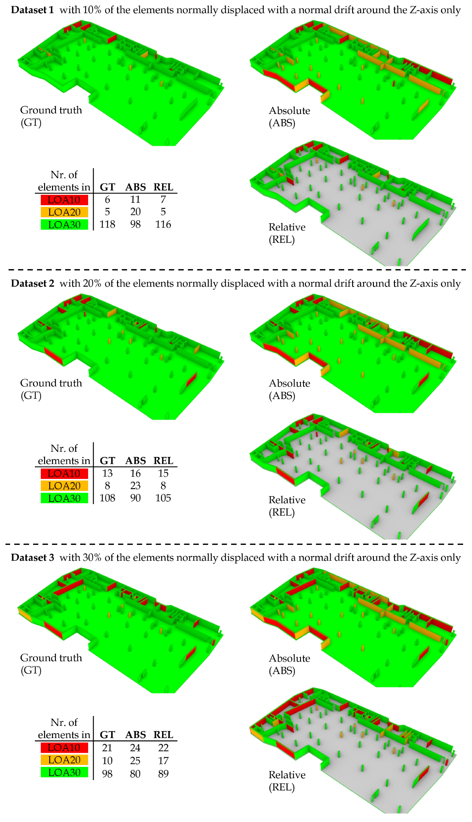
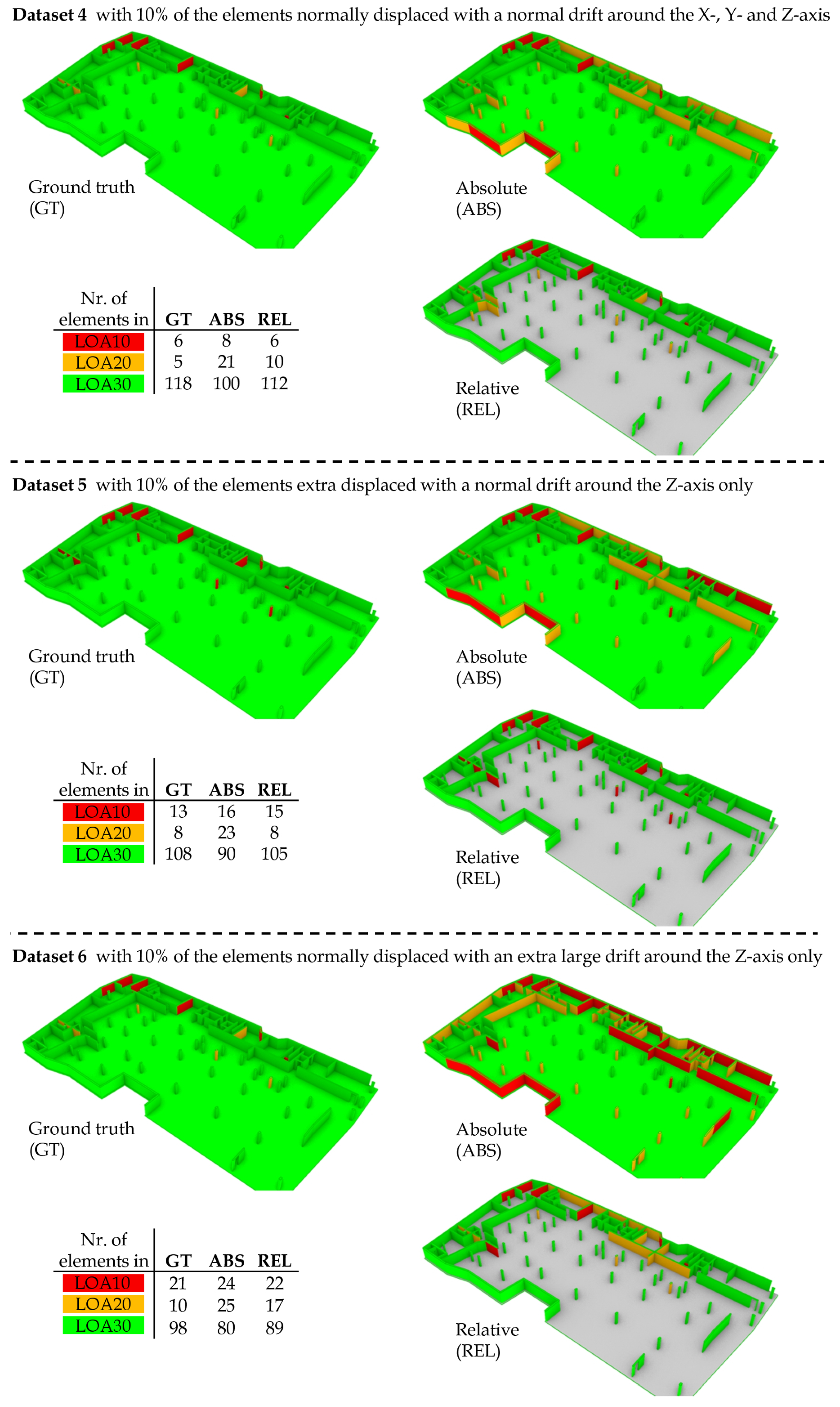
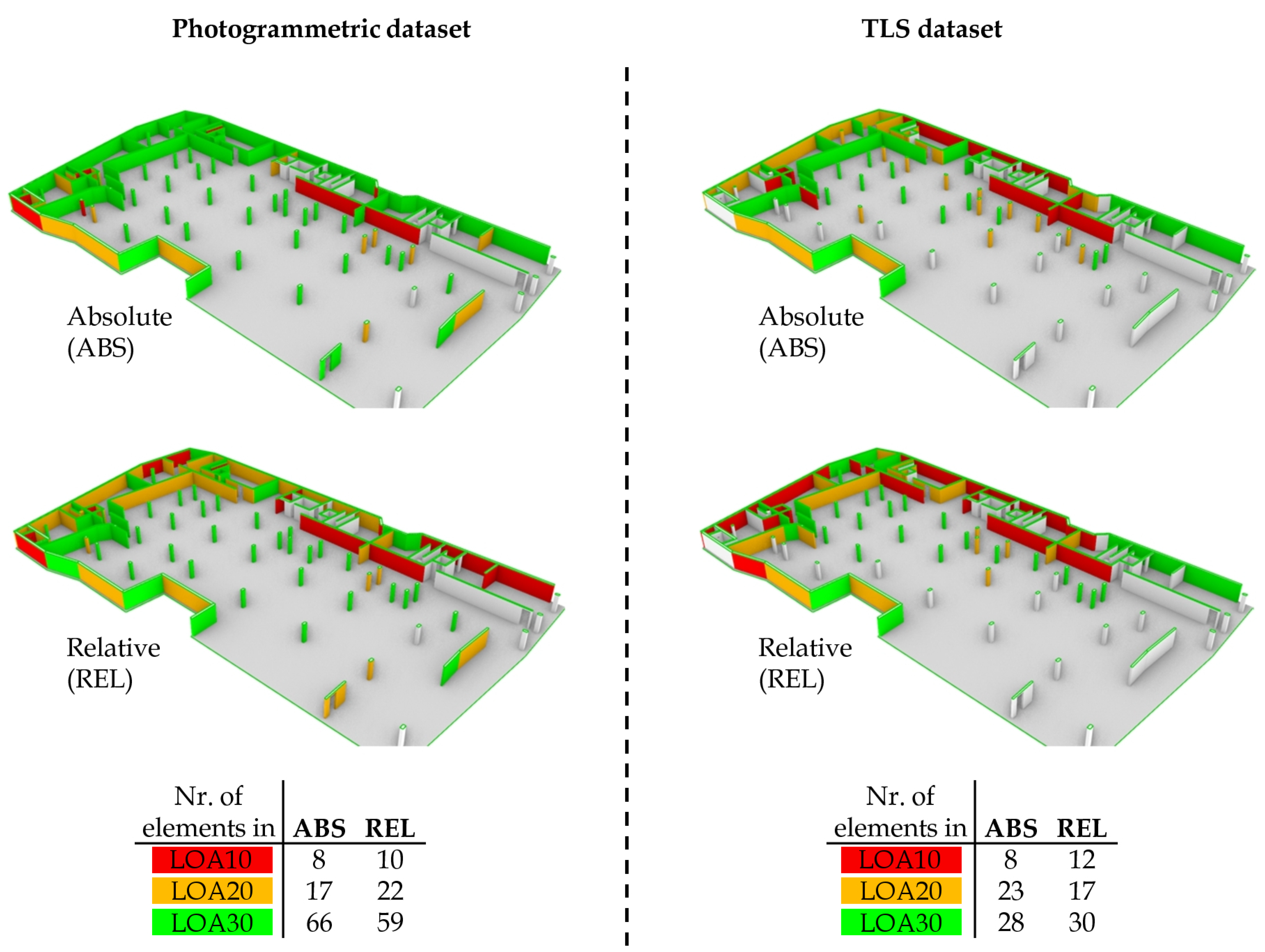
Using the described approach that subdivides the construction site in smaller parts for a locally more correct alignment, a series of experiments are performed on the 6 discussed datasets. It is chosen to also visually output the results by coloring each of the elements according to its adjusted error vector coupled to the LOA ranges. The colored assessment results are presented in Figure 5 and Figure 6. They show both the result of the currently conventional absolute analysis as well as the proposed relative analysis alongside the ground truth data. Furthermore, a numerical representation is also included where the number of elements per LOA class is depicted. It should be noted that the floor slab is not considered in all of the relative analyses. it spans the entire construction site and thus is so large that it suffers from internal drift, which cannot be compensated. Therefore it is colored gray in all visual results and excluded from the resulting tables.

The validity of our approach is clearly reflected in the figures: all erroneously placed elements are detected as faulty. Overall, in almost all of the cases the assigned LOA class is correct. Furthermore, it can be noted that each of the incorrectly located elements is assigned to the correct class or the one above (i.e., the class with worse results). On the downside however, also several other elements are considered as faulty, despite their correct placement. When considering the separate analyses, it can be noted that a value of 30% incorrectly placed elements yields slightly worse results compared to 10% and 20%. However, it is rather unlikely to encounter a site where 30% of the elements are severely displaced. In contrast to the absolute method, the analyses point out that the proposed approach is still valid even when applying a larger drift or element displacement.

As we opted for a colored analysis visualisation according to the LOA ranges, the results are arguable. The LOA ranges are quite broad, hence elements with a rather large difference in error can still be assigned to the same class. Therefore, we also assess the adjusted error vectors that lay at the basis of the visualisation. The magnitude of the error vectors on the 6 datasets are shown in

Table 2. Overview table of the error vectors for a subset (5 out of the 129) of representative elements alongside the overall median and standard deviation (sd) values. For simplicity reasons all error vectors were transformed to a singular root-mean-square error (RMSE) value.

Error Vector (mm)	Dataset 1					Dataset 2
element nr.	GT	ABS	ΔABS	REL	ΔREL	GT	ABS	ΔABS	REL	ΔREL
overall median			6		0			6		1
overall sd			15		5			14		5
8	0	63	63	3	3	0	62	62	3	3
23	0	8	8	0	0	0	8	8	0	0
28	0	13	13	0	0	0	13	13	0	0
84	0	46	46	51	51	0	45	45	51	51
108	0	6	6	0	0	0	6	6	3	3
	Dataset 3					Dataset 4
element nr.	GT	ABS	ΔABS	REL	ΔREL	GT	ABS	ΔABS	REL	ΔREL
overall median			7		1			6		0
overall sd			14		12			11		5
8	0	61	61	3	3	0	45	45	2	2
23	0	9	9	0	0	0	6	6	0	0
28	0	13	13	18	18	0	9	9	0	0
84	0	45	45	51	51	0	36	36	24	24
108	0	7	7	10	10	0	6	6	0	0
	Dataset 5					Dataset 6
element nr.	GT	ABS	ΔABS	REL	ΔREL	GT	ABS	ΔABS	REL	ΔREL
overall median			6		0			12		1
overall sd			14		5			48		13
8	0	63	63	3	3	0	214	214	11	11
23	0	9	9	0	0	0	25	25	1	1
28	0	13	13	2	2	0	48	48	0	0
84	0	46	46	51	51	0	129	129	135	135
108	0	6	6	0	0	0	9	9	0	0

.

For a realistic dataset (Dataset 1), very decent results are obtained. Moreover, also in the more challenging datasets (Dataset 2–6) the proposed framework performs quite well. A median difference in the error vector of our approach versus the ground truth of 1 mm is obtained (with rather high standard deviations ranging from 5 to 13 mm, mostly due to a small number of rather severe outliers) for all datasets, even the highly deformed ones. Our method also vastly outperforms the traditional absolute method with respective differences ranging from 6 to 12 mm (with standard deviations ranging from 11 to 48 mm). When considering the individual elements and their results, element number 23, 28 and 108 are the most representative for the executed assessments. These elements are respectively a medium size wall (approximately 4 meters), a column and a small wall (approximately 2 meters) and are spread over the scene. Relatively decent results are obtained for the absolute analysis and even better results are achievable with the proposed relative analysis. Roughly 80% of the data has similar values for the absolute and relative analyses as these 2 elements. An excellent example can be found for element number 8, a medium sized wall, where the absolute analysis performs very bad while our method yields acceptable results. For some elements, both analyses underperform. In general it can be stated that our method performs well for small to medium-sized object. However in some cases, anomalies arise. Mostly this is due to either large (erroneous) elements in the close neighborhood that highly influence the results of the surrounding smaller elements, a group of neighbouring elements that are all located erroneously in the same direction (i.e., all translated for approximately the same distances along x- and y-axis) or due to a relative small number of points on the element. Furthermore it can be noted that in rare cases such as for element 84, a medium sized wall, the relative method scores worse than the absolute analysis. When comparing different dataset results it becomes clear that the worst results are obtained in dataset 6 (large drift) for the absolute method and likewise dataset 6, closely followed by dataset 3 (30% displaced elements) for the relative method.

In conclusion it can be stated that for all datasets our approach proves beneficiary over the conventional method. It is able to detect all incorrectly placed elements, although a small set of correct elements also is determined as faulty, ranging from approximately 1% in the more realistic datasets to a maximum of 6% in the heavily tweaked datasets. Therefore it can be noted that our method is rather overshooting. However, when coupling back to the purpose of the analysis, namely metric quality control for effective construction site monitoring, overdetection is preferable over underdetection. When incorrect elements are not detected when assessing the site at a specific moment, the consequences of their erroneous placement are likely to be noticed later on in the building process. However, the later in the construction process, the higher the repair or modification costs.

5.3. Realistic Data

We also executed experiments on actual recorded data. As our method is sensor-independent, it works both for photogrammetric point cloud data as well as the data recorded with a terrestrial laser scanner. The photogrammetric dataset is constituted based on a total of 1453 images spread over the scene. Moreover, a terrestrial laser scanning dataset was also recorded. A total of 19 scans are aligned via the cloud-to-cloud technique. Both datasets are registered in the same coordinate system as the BIM model. Via total station measurements and a set of surveyor points used for the stake-out of the buildings, a new set of Ground Control Points (GCPs) on the surrounding facades is determined in coordinates. In turn, these GCPs enable the registration of the photogrammetric dataset in the BIM model reference system. This is ensured via a pre-registered reference module that incorporates the correct coordinate system. The followed method is described in depth in previous work [8]. The laser scanning dataset is registered via the traditional method of indicating ground control points. The subsequent quality assessments of both resulting datasets by the absolute and relative methods are presented in Figure 7. In contrast to the synthetic data experiments, it is noted that the proposed framework provides similar results as the absolute method under the assumption that every object was correctly built. Partial or complete occlusions of elements due to the cluttered environment (as displayed in Figure 2) play a major role in this phenomenon. Occlusions cause sparser PCD that in turn makes it harder to correctly align two smaller datasets compared to larger ones as fewer correspondences are present. Moreover, in the considered remote sensing datasets, some elements are not yet completed (e.g., molding of an in-situ cast concrete wall). In future work, it is therefore required to first assess the element’s state and subsequently only perform the analysis on the finished elements.

No ground truth data for the captured datasets is available, hence the only meaningful assessment is the comparison between the achieved results for both dataset types. It is remarkable that, despite the larger amount of points for the TLS dataset (2.5 million) in comparison to the photogrammetric dataset (1.7 million), the total number of elements that are considered for the quality assessment is significantly lower for the TLS dataset (59) compared to the photogrammetric dataset (91). Although the photogrammetric dataset consists of a lower number of points, these are to be found more on the element surfaces compared to TLS. This shows that state-of-the-art photogrammetric technologies can compete with low-level laser scanners in terms of accuracy and can also be used for quality control tasks. A driving factor in the poor lidar results is the noise caused by mixed-edge pixels and ghosting which is less of a problem in photogrammetric processes.

A second remark is that a significant portion of the larger elements is considered as erroneously located in the relative assessments and in a lesser extent also in the absolute assessment of the TLS dataset while the opposite is the case for the vast majority of the smaller elements. It is assumed that for large elements such as some of the present walls of $30m$ and more, internal drift effects start to play a role. Another remark is that some elements are determined as correctly built and thus assigned to LOA30 in one dataset while these contrastingly are assigned to the erroneous LOA10 class when assessing the other dataset. It can be concluded that this tells more on the recorded data quality than the actual (in)correct location of elements.

6. Discussion

In this section, the pros and cons of the procedure are discussed and compared to the alternative methods presented in the literature. A first major aspect in the error assessment is the data association between the observed and as-design shape of the objects that is, which point correspondences are used for the detection and evaluation. As stated in the literature study, there are three strategies relevant to this work that is, absolute, relative and descriptor-based correspondences. Absolute methods such as presented by Bosche et al. [9] reach sub-centimeter accuracy with correctly positioned point cloud data. However, if this is not the case, our method, based on the relative positioning, clearly outperforms the absolute evaluation as it accounts for drift and (geo)referencing errors that can reach up to 15cm for mobile systems [26]. However, at its core, ICP is unintelligent and can be outperformed by descriptor-based correspondences such as ORB or SHOT. Especially for objects with significant detailing, descriptors have proven to be very successful with reaching sub-centimeter accuracy in realistic conditions [58]. However, the photogrammetry and lidar datasets reveal that discriminative points near the object’s edges or corners are systematically occluded and error prone as the as-design shape frequently is an abstraction of the constructed state.

A second aspect is the accuracy of the remote sensing inputs. Given perfect data, an absolute comparison is the most straightforward and suitable solution to perform a reliable quality control. One might expect that this accuracy is a given with the ongoing sensor advancements but current trends beg to differ. Construction site monitoring and qualitative quality control will remain challenge due to the speed and low budget by which these tasks must be performed. As such, future work will investigate to which extent that low-end sensors, enhanced through relative positioning, can be deployed for metric quality control on construction sites. This requires a deeper understanding of the drift effects that currently plague construction sites which is understudied in the literature. Overall, if fast quality control can be achieved with affordable low-end sensors, the impact on construction validation will be enormous. In future work, we will therefore study the decrease in construction failure and failure costs to fuel the valorization of this technology.

A third aspect is the validity of the rigid body transformation assumption. In the presented method, it is hypothesized that a single rigid body transformation can be defined for every object. It builds upon the assumption that the error propagation in the registration of consecutive sensor setups is negligible for a single object. While the experiments prove that this is correct, it does not apply to extremely large objects. For instance, the floor slab and some of the larger walls in the experiments span over the entire project and thus are subject to drift. This internal drift is currently not accounted for in the presented method and is part of future work. A possible solution is to discretize the objects into sections and treat each section individually. This will provide a more nuanced error and progress estimation for large objects that are typically built in different stages.

A fourth aspect is the error vector definition. The LOA specification prescribes LOA ranges for the $95\%$ confidence intervals of the errors. However, this applies only to observations that actually belong to the target object, which are challenging to isolate in cluttered and noisy environments that are construction sites. Moreover, since the objective is to track positioning errors, our method defines a search area in which every observation is considered regardless of its association to the target object. As a result, the LOA inliers are littered with false positives that negatively impact the error assessment. In the literature, the average, the median and even the $70\%$ value of the Euclidean distances between the correspondences have been reported, which are incorrect as they include the noise, false positives, registration errors, (geo)referencing errors and even the resolution of the point cloud. In contrast, we base our error vectors on the ICP transformations which correctly report the positioning errors but are sensitive to occlusions and clutter. This is compensated in the score function for the dominant transformation that considers the transformation resistance and the object’s occlusions, leading to very promising results.

Aside from the pros and cons, there are important limitations of the method to consider. First of all, there is the scalability of the method. The initial segmentation with a linear computation complexity makes the method very efficient but each new object still has to be tested against the entire point cloud, rendering larger projects unfeasible. Also, the method currently does not deal with internal drift which will be solved through discritization in future work. Third, the error vector representation along the cardinal axes is less suited for more complex and larger objects. In future work, we will study a Principal component analysis (PCA)-based representation and how object discritization can lead to more intuitive error vectors. Lastly, the method prefers the impact of larger objects which might not necessarily be placed more correctly. Furthermore, also limitations in the conducted experiments exist. So far the proposed method was assessed based upon synthetic data for a number of good reasons as described earlier. However, more elaborate future assessments are essential to verify the method’s validity when performing analyses with actual recorded data. For instance, the influence of (severe) occlusions, absent in the synthetic dataset, is still an understudied subject. However, key to such recorded data experiments is a very accurate ground truth dataset, unavailable in our experiments so far, that serves as comparison and evaluation.

7. Conclusions & Future Work

In this paper, a novel metric quality assessment method is proposed to evaluate whether built objects on a construction site are built within tolerance. The presented two-step procedure computes the systematic error vector of each entity regardless of sensor drift, noise, clutter and (geo)referencing errors. In the first step, the individual positioning error of each object is determined based on ICP. However, as this is error prone due to occlusions, uneven data distributions and the above errors, the surroundings of each object are also considered. In the second step, we therefore establish a dominant transformation in the vicinity of each object and compensate the object’s initial error vector with this transformation, thus eliminating the above described systematic errors. The resulting adjusted positioning error is reported with respect to the Level of Accuracy (LOA) specification. In this work, LOA10, 20 and 30 are considered which form the common range of construction site tolerances and their errors. Notably, the method relies on a spatial data association in the first step and thus the initial point cloud should be (geo)referenced with a maximum error equal to the search area around each object. This research will lead to lower failure costs as errors are detected in an early stage where they can be mitigated without expensive building adjustments.

The method is tested on a variety of test sites. First, the method’s performance is empirically determined and compared to a traditional error assessment. To this end, a simulated dataset is generated from an actual construction site with a fixed ground truth and systematically introduced errors that represent the drift, (geo)referencing and actual positioning errors. Next, the outputs of our method and the traditional method are compared for actual construction site measurements obtained by photogrammetry and lidar. Overall, the experiments show that the presented method significantly outperforms the traditional method. Its ability to mitigate noise, drift and (geo)referencing errors results in a more realistic error assessment, which is vital to help stakeholders reduce failure costs. However, some errors still remain such as the internal drift of massive objects for example, a floor slab that spans over the entire construction site does not comply with the rigid body transformation assumption and will therefore be error prone.

The future work includes the preparation for valorization by increasing the method’s robustness and ability to process different types of sensor data. Also, it will be studied to which degree failure costs are lowered by periodic quality control no construction sites. On the scientific front, we are studying the discretization of the input BIM objects to mitigate internal drift, the implementation of a dynamic search radius to establish the dominant transformation and also an automated georeferencing procedure which currently is frequently overlooked in the state of the art. Additionally, we are investigating the opportunities to asses internal object dimensions regardless of the object’s type or shape given the error vectors.