Monitoring of Urban Growth Patterns in Rapidly Growing Bahir Dar City of Northwest Ethiopia with 30 year Landsat Imagery Record

Abstract

Monitoring urban growth patterns is an important measure to improve our understanding of land use/land cover (LULC) changes and a central part in the proper development of any city. In this study, we analyzed the changes over a period of 30 years (1985–2015) in Bahir Dar, one of the rapidly growing cities of northwest Ethiopia. Satellite images of Landsat TM (1985, 1995, and 2008), and OLI (2015) were used. The classification was carried out using the object-based image analysis technique and a change analysis was undertaken using post-classification comparison in GIS as a novel framework. An accuracy assessment was conducted for each reference year. Eight LULC types were successfully captured with overall accuracies ranging from 88.3% to 92.9% and a Kappa statistic of 0.85 to 0.92. The classification result revealed that cropland (66%), water (12.5%), and grassland (6%) were the dominant LULC types with a small share of areas covered by built-up areas (2.4%) in 1985. In 2015, cropland and water continued to be dominant followed by built-up areas. The change result shows that a rapid reduction in natural forest cover followed by grassland and wetland occurred between the first (1985–1995), second (1995–2008), and third (2008–2015) study periods. On the contrary, build-ups increased in all three periods by 9.3%, 121.3%, and 44.8%, respectively. Although the conversion between the LULC classes varied substantially, analysis of the 30-year change matrix revealed that about 31% was subject to intensive change between the classes. Specifically, the built-up area has increased by 250.5% during the study years. The framed approach used in this research is a good repeatable example of how to assess and monitor urban growth at the local level, by combining remote sensing and GIS technologies. Further study is suggested to investigate detailed drivers, consequences of changes, and future options.

1. Introduction

Monitoring urban growth patterns, generally based on land use/land cover (LULC) changes, is one of the major global research themes in terms of urbanization [1]. Excessive urbanization affects the survival and development of human society and ecosystems [2,3], and its consequences involve the transformation of natural forms of land cover into urban areas [4], effects on genetic diversity [5], an increased disease burden [6], heat island effects [7], and greenhouse gas emissions [8]. Therefore, timely and accurate acquisition of urban LULC distribution can serve as the basis for assessing and mitigating these negative socio-economic-ecological impacts [2,9].

With an area of 1,130,000 km², Ethiopia is one of the five most populous countries in the African continent and among the fastest urbanizing countries in the world [10]. In Ethiopia, urban growth patterns are constantly changing, while land is gradually becoming a scarce resource [2,9,11,12]. The intensity and magnitude of urban growth patterns vary in different cities across the country. For example, Nigatu et al. [13] reported an increase in urban areas of Hawassa in southern Ethiopia by 185.4% in 16 years (1995–2011), while, Fenta et al. [14] reported an increase in the built-up area of Mekelle city in northern Ethiopia by 88% in 30 years (1984–2014). Consequently, making generalizations of the results to other areas for any planning activity may lead to erroneous conclusions. Results of various studies have demonstrated that improving knowledge on urban growth will have a high impact on the design of appropriate management strategies. Specifically, it will guide urban planners and decision makers in what approaches would be appropriate to tackle land cover changes and uncontrolled urban growth [15]

Earlier research on urban LULC changes based on ground surveys or statistics encountered difficulties with capturing and monitoring speedy urbanization. Accurate, consistent, and timely data on trends in urban growth are needed for assessing current and future needs [16,17]. With the advent and development of geospatial techniques that integrate the use of remote sensing (RS) and a geographic information system (GIS), the detection of spatio-temporal LULC dynamics has become easy, quick, and cost-effective [18,19].

Various techniques are available to extract meaningful information on LULC types from remotely captured datasets. In the past, most LULC classifications have been created using a pixel-based analysis of remotely sensed imagery. Recently, object-based image analysis (OBIA) has been applied more frequently for remote sensing image classification than the pixel-based analysis technique, e.g., [20,21,22]. Pixel-based methods mainly classify individual pixels using spectral patterns. On the other hand, OBIA allows the combination of both spectral information and spatial information to accurately classify LULC types [23,24,25]. The novelty of OBIA brings the ability to group relatively homogenous pixels into meaningful objects based on their spectral values through the use of a multiresolution segmentation algorithm, and then extract useful extra information such as size, shape, texture, or contextual information [20]. Moreover, the OBIA approach enables us to separate spatially and spectrally similar pixels at different scale levels [26]. To the best of our knowledge, there are hardly any approaches better than OBIA for producing repeatable local level urban LULC classifications that can be used as input for monitoring and planning.

However, the accuracy of the object-based approach differs depending on the nature of the study area, level of details, and the type of images used for analysis [21,27,28,29]. Considering that, in this study, we classified the LULC types using OBIA with the highest possible accuracy and evaluated changes over a period of 30 years (1985–2015) in Bahir Dar, one of the rapidly growing cities in Ethiopia.

2. Materials and Methods

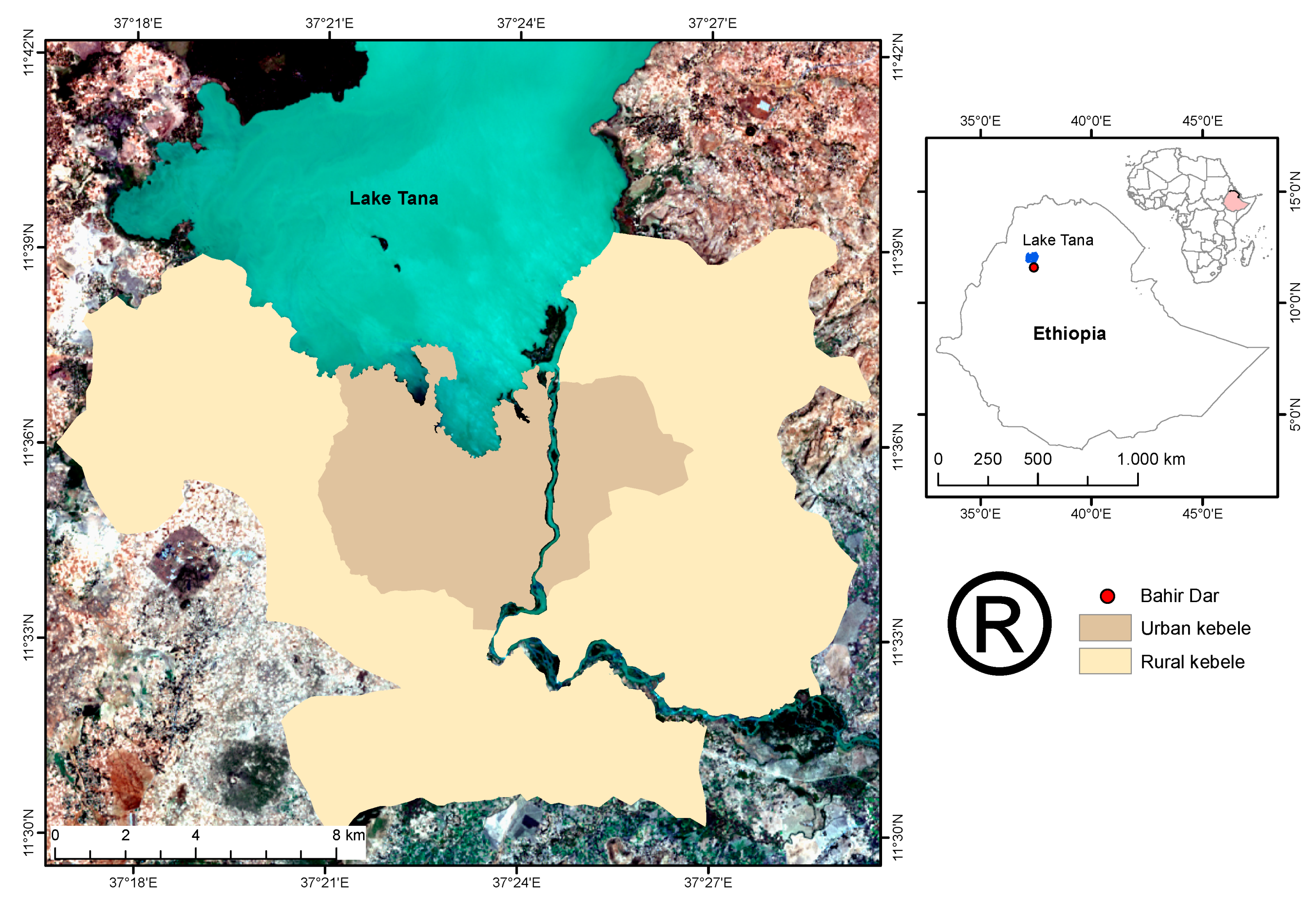
2.1. Study Area

Bahir Dar town (meaning “sea shore” in Amharic) is the capital city of the Amhara National Regional State and the seventh largest city in Ethiopia. It is located in the northwestern highlands of Ethiopia at 11°35′41.2″ N and 37°23′17.2″ E (Figure 1). The city is settled on the banks of Abay (the Blue Nile—the longest river in the world), right after the river flows out of Lake Tana, which is the source of its beauty. It has both rural and urban kebeles, which are the smallest and lowest level of administration units in Ethiopia. The urban kebeles of the city size is only about 1.5% as compared to size of Lake Tana surface area (which is ca. 3111 km²). The city is situated 565 km northwest from the capital city Addis Ababa and has an average altitude of 1830 m. In 2002, Bahir Dar was awarded the UNESCO Cities for Peace Prize for successfully addressing the challenges of rapid urbanization [30]. Bahir Dar falls within the Woina Dega climatic zone, which is characterized by a rainy season (from May–October) and dry season (October–May). The mean annual atmospheric temperature ranges between 15–21°C. The rainfall has a normal distribution with a maximum in July and August (396 mm and 375 mm, respectively) and a minimum in January and February (2 mm for both months). The total annual rainfall for 2015 was 1416 mm [31]. The main soil types are clays and silty clays.

The modern and comprehensive master plan, which directed the current shape of the city though new zoning, was prepared in 1965 by a team led by a German expert. The implementation of this master plan has changed the physical appearance of Bahir Dar (Figure 2). A revised master plan has been made effective since 2005 [30]. According to the last population census in 2007, Bahir Dar town had 185,933 inhabitants, of whom 83.6% (155,428 people) lived in urban areas and 16.4% (30,505 people) lived in rural areas around the city [32].

2.2. Data Used

2.2.1. Satellite Imagery

Satellite images for 1985, 1995, and 2008 from Landsat 5 Thematic Mapper (TM), and for 2015 from Landsat 8 Operational Land Imager (OLI) were acquired from the United States Geological Survey (USGS) website. The images were downloaded as standard surface reflectance products at Level 1T with applied radiometric corrections. They were then geometrically referenced to the World Global System 1984 (UTM zone 37 projection system). The only exception was the Landsat 5 TM image for 2008 which demonstrated some geometric distortions and anomalies. In this case, geometric corrections were performed in order to enhance the 2008 image by applying geocoding and geo-referencing algorithms in PCI Geomatica Version 2015 SP1.

The reference years were determined based on major regimes and policy changes in the study site. The satellite images were also selected based on four criteria: season, acquisition time, cloud cover, and data availability. All the images were acquired in February for dry season analysis. The images were intentionally chosen from the same months and season to decrease discrepancies in land cover due to seasonal changes.

2.2.2. Other Datasets

Other datasets required for this study were collected through both primary and secondary sources. Field observation was conducted in January 2016 in order to collect reference data for the accuracy assessment, and to verify the results from the change detection study. Ground truth data was acquired using GPS GARMIN Montana 600 during the direct field observation study in January 2016. A total of 124 reference samples, including different LULC types, were collected on the site, based on the simple stratified method—main market areas, central business district (CBD), city center, bus stops, health centers, educational institutions, urban agriculture, and wetlands. Those samples were further used to assess the accuracy of the land cover map from 2015.

Secondary datasets, such as administrative boundaries, water bodies, road networks, public services, and aerial photography were mainly collected from different sources.

2.3. Methodology

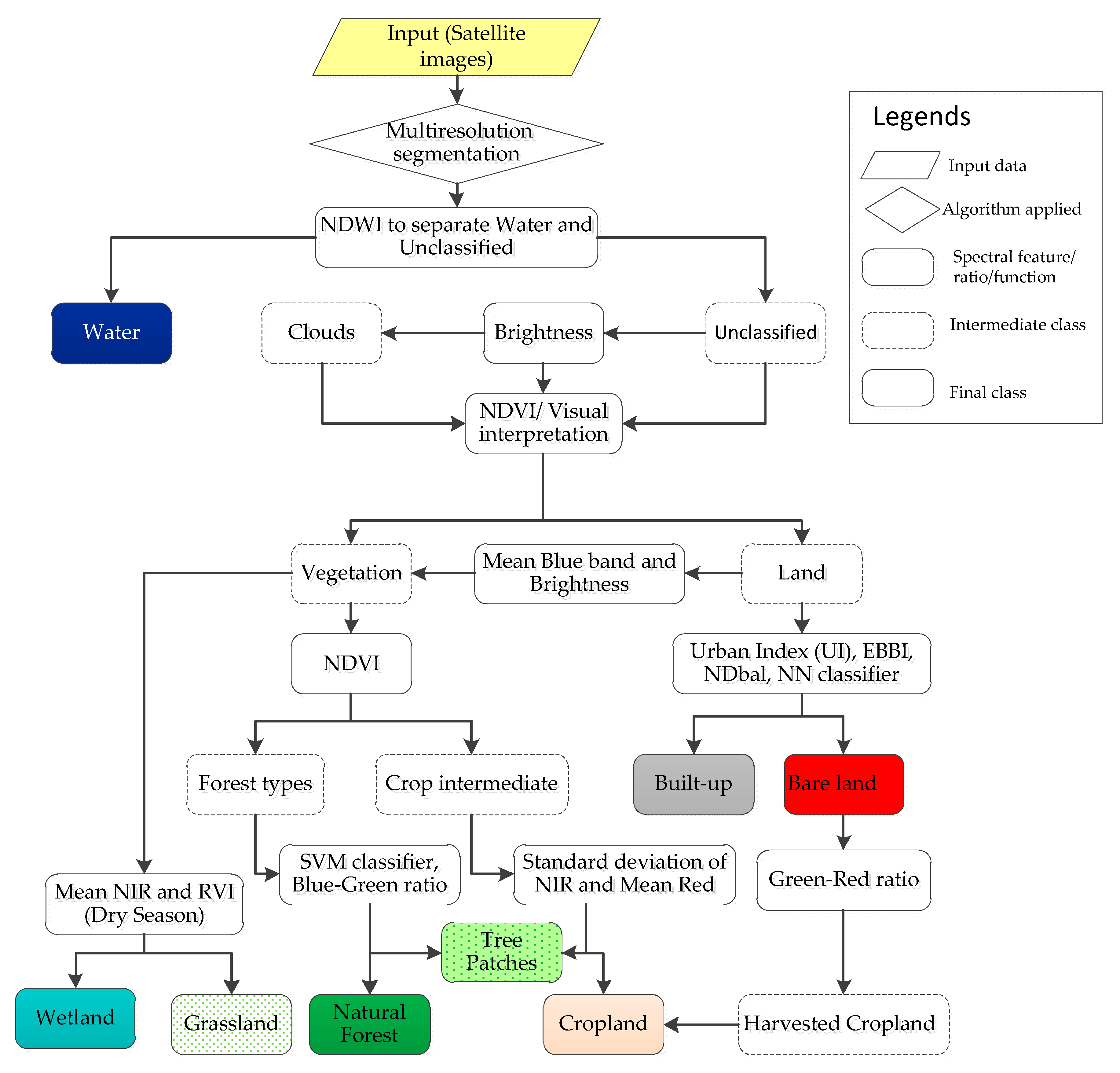
2.3.1. Image Segmentation and Classification

Eight LULC classes were used during the image classification process: bare land, cropland, grassland, built-up, natural forest, tree patches, wetland and water (

Table 1. Description of land use/land covers classes used for change study from 1985 to 2015.

LULC Class	Description
Bare land	Areas with less than 10% vegetated cover during any time of the year, which are degraded due to erosion, intensive traditional cultivation of crops, or over grazing (including exposed stone, sand, and soil) [33].
Cropland	All areas designated for crop cultivation. During the dry season (October–May), some of the cropland turns into harvested land which is part of the cropland class by definition.
Grassland	This is land dominated by grass cover.
Built-up	All types of artificial surfaces including: residential and commercial areas, transportation networks, industrial areas, infrastructure, and all types of urban features.
Natural forest	Deciduous forests which have a minimum land area of 0.5 ha with a tree canopy cover of more than 10%, which is not subject to agricultural or other specific non-forest land use [33].
Tree patches	A group of trees with an area smaller than 0.5 ha which includes bush and shrub lands.
Wetland	Non-forested areas either partially, seasonally, or permanently waterlogged. The water may be stagnant or circulating [34].
Water	Lakes, rivers, ponds, and all kinds of water bodies.

).

The study used a multistep approach to investigate the LULC changes in Bahir Dar town during the 1985–2015 period. First, the LULC of the different reference years were extracted as shown in Figure 3, following the general approach of Kindu et al. [29] using eCognition Developer 9.2.1 software [35].

A multiresolution segmentation (MS) algorithm was applied during the first step of the classification process to identify appropriate segmentation parameters for each of the used images. The MS algorithm is an optimization procedure that minimizes the average heterogeneity for a given number of objects and maximizes their homogeneity based on defined parameters. These parameters, namely scale, shape, and compactness, are defined through an iterative “trial and error” approach to successfully segment objects in an image [29,36,37]. Different combinations of scale parameters, ranging from 10 to 100, shape, and compactness values were used for each image to properly separate the image objects (

Table 2. Segmentation parameters applied in the different images.

Parameters	1985 (Landsat 5 TM)		1995 (Landsat 5 TM)		2008 (Landsat 5 TM)		2015 (Landsat 8 OLI)
	Level 1	Level 2	Level 1	Level 2	Level 1	Level 2	Level 1
Scale	20	10	15	10	15	10	100
Shape	0.1	0.1	0.2	0.1	0.2	0.3	0.3
Compactness	0.5	0.5	0.5	0.5	0.5	0.5	0.7

). The images from L5TM (for 1985, 1995, and 2008) were classified based on a two-step segmentation workflow, where the water class was separated from land and vegetation on the first level, and all the other LULC classes were delineated on the second level (Figure 3). However, the 2015 image from L8 OLI used a single segmentation level, as the scale, shape, and compactness parameters provided enough detail for delineating all the LULC classes on Level 1 so that no additional level was needed.

After the segmentation was processed, a normalized difference water index (NDWI) was calculated. This index was defined by McFeeters [38] and it aims to delineate open water features and enhance their presence in remotely-sensed digital imagery. It calculates the difference between green and near–infrared (NIR) wavelengths, divided by their sum:

$$\mathrm{NDWI}= \frac{{\mathrm{X}}_{\mathrm{Green}}{-\mathrm{X}}_{\mathrm{NIR}}}{{\mathrm{X}}_{\mathrm{Green}}{+\mathrm{X}}_{\mathrm{NIR}}}$$

(1)

where ${\mathrm{X}}_{\mathrm{Green}}$ = green wavelength and ${\mathrm{X}}_{\mathrm{NIR}}$ = NIR wavelength.

As a result, the water was differentiated from all other classes which were grouped in the unclassified class.

Clouds were detected in the rainy season images from 2008 and 2015 as they had considerably higher brightness values. They were later reassigned to either vegetation or land by using historical imagery from Google Earth for the 2008 image and visual interpretation of the dry season image in 2015.

Next, land and vegetation classes were distinguished by using the normalized difference vegetation index (NDVI). In general, lower values of NDVI indicated land, and higher values indicated healthy vegetation. The index uses the difference between the NIR and red wavelengths, divided by their sum:

$$\mathrm{NDVI}= \frac{{\mathrm{X}}_{\mathrm{NIR}}{-\mathrm{X}}_{\mathrm{Red}}}{{\mathrm{X}}_{\mathrm{NIR}}{+\mathrm{X}}_{\mathrm{Red}}}$$

(2)

where ${\mathrm{X}}_{\mathrm{NIR}}$ = NIR wavelength and ${\mathrm{X}}_{\mathrm{Red}}$ = Red wavelength.

After the NDVI index was computed, some vegetation objects were wrongly classified as land. To correct this, the values of the mean Blue Band (Band 1 for L5TM and Band 2 for L8 OLI, respectively) and brightness were used to reassign them to the vegetation class.

The rest of the land was classified as bare land or built-up area using the nearest neighbor (NN) classifier and several different indices: urban index (UI), enhanced built-up and bareness index (EBBI), and normalized difference bareness index (NDBaI) (

Table 3. Different index applied for delineation of bare land and built-up area classes.

Index/ Classifier	Year	Description
Urban index	1985 (L5TM)	Observes the relationship between near infrared and mid infrared wavelengths to detect built-up areas.
NN Classifier	1995 (L5TM)	Sample selection based on: Bands 3, 4, 1 (Red, NIR, Blue) Bands 3, 5, 7 (Red, SWIR 1, and SWIR 2) Bands 5, 4, 1 (SWIR 1, NIR, and Blue)
	2015 (L8 OLI)	Mean Blue values (Band 2)
EBBI	2008 (L5TM)	Measures the contrast reflection range and absorption in built-up and bare land areas [39].
NDBaI	2015 (L8 OLI)	Used to map bare land, based on the significant difference of spectral signature in the NIR between bare land and the other LULC classes [40].

). Each of these indices performed differently in terms of precision when delineating the classes due to the different satellite imagery. Table 3 presents the index applied in the specific year to distinguish bare land from the built-up class.

The application of the indices varied in the classification of the different satellite images. For instance, the UI was applied to the classification of those from 1985. Furthermore, the NN classifier was used to distinguish between built-up and bare land in the image classification of 1995, by combining different bands such as: mean red, NIR, and Blue values (B3, B4 and B1 for L5TM), as well as Red, SWIR I, SWIR II (B3, B5, B7 for L5TM), and SWIR I, NIR, and Blue (B5, B4, B1). EBBI was used to separate built-up from bare land in the image classification of 2008.

The UI, developed by Kawamura et al. [41], observes the relationship between near infrared and mid infrared wavelengths:

$$\mathrm{UI}=\frac{\mathrm{Band} 7-\mathrm{Band} 4}{\mathrm{Band} 7+\mathrm{Band} 4}$$

(3)

$$\mathrm{EBBI}=\frac{\mathrm{Band} 5-\mathrm{Band} 4}{10\sqrt{\mathrm{Band} 5+\mathrm{Band} 6}}$$

(4)

$$\mathrm{NDBaI}=\frac{\mathrm{Band} 5 - \mathrm{Band} 10}{\mathrm{Band} 5 + \mathrm{Band} 10}$$

(5)

where Band 7 (SWIR 2) and Band 4 (NIR) are represented by the digital numbers (DN) in the respective wavelength of Landsat 5 TM; Bands 4, 5, and 6 represent NIR, SWIR1, and TIR, respectively, from Landsat 5 TM; Bands 5 and 10 represent NIR and TIRS1, respectively, from Landsat 8 OLI.

In comparison to UI, the EBBI showed a better performance when classifying the bare land and built-up areas in the 2008 image. This index was developed by As-syakur et al. [39]. It is based on the contrast reflection range and absorption in built-up and bare land areas. The normalized bare soil index (NDBaI) was applied in the 2015 image to delineate bare land from the other LULC classes [40]. Although the NDBaI gave good results when separating the bare land class in the 2015 image, refinement was needed. Therefore, samples from both classes were selected based on their Mean Blue values (Band 2 in L8 OLI). Eventually, the NN classifier was applied to separate both classes.

In the 1995 dry season image, the bare land was overestimated at the expense of cropland. For that reason, a Green-Red ratio was computed in order to reassign the misclassified bare land objects to a temporally created intermediate harvested cropland class which, by default, belongs to the cropland class as suggested by Kindu et al. [29].

It was essential to distinguish both classes because during the dry season, harvested cropland appears as bare land. Therefore, the Green-Red ratio was used because a visual interpretation of the dry season image (the only one available for 1995) was not enough for delineation of the classes. In general, bare land had lower values, and the opposite was true for harvested cropland. The formula used for the computation of this ratio was:

$$\mathrm{Green}-\mathrm{Red} \mathrm{ratio}=\frac{\mathrm{Mean} \mathrm{Green}}{\mathrm{Mean} \mathrm{Red}}$$

(6)

where the DN of Band 2 (Mean Green) are divided by the DN of Band 3 (mean red) from Landsat 5 TM. Subsequently, the harvested cropland was directly reassigned to the cropland class.

Two different forest types were identified throughout the image classification process, namely natural forest and tree patches. A support vector machine (SVM) classifier was used in order to delineate the classes by comparing values within the Blue-Green ratio [29]. SVM is one of the machine learning methodology that analyze data and recognize patterns, used for classification and regression analysis [35]. It is based on the decision planes that separates between a set of objects having different memberships. Depending on the size of classes a minimum of 30 training samples (object primitives) per class were used. The radial basis function kernel was used as it is the most popular choice in SVMs [35,42].

$$\mathrm{Blue}-\mathrm{Green} \mathrm{ratio}=\frac{\mathrm{Mean} \mathrm{Blue}}{\mathrm{Mean} \mathrm{Green}}$$

(7)

Natural forest appeared to have higher values compared to tree patches. The classification of tree patches was improved based on their area (generally smaller than 0.5 ha) and finer texture.

The cropland intermediate class was further subdivided into cropland and tree patches based on their standard deviation of NIR and Mean Red values. Tree patches demonstrated lower values in both domains, compared to cropland.

Finally, a spectral feature of Mean NIR and a ratio vegetation index (RVI) were calculated in order to delineate grassland and wetland from the vegetation class. The ratio was calculated as follows [43]:

$$\mathrm{RVI}=\frac{\mathrm{Mean} \mathrm{NIR}}{\mathrm{Mean} \mathrm{Red}}$$

(8)

Grassland demonstrated higher values in the Mean NIR domain and lower values in the RVI than wetland.

2.3.2. Accuracy Assessment

Accuracy assessment evaluates the reliability of the results from the classified map and assures confidence in the product by deploying a confusion matrix [44]. Four accuracy assessment confusion matrices were produced to evaluate the classification results and characterize errors from 1985, 1995, 2008, and 2015 maps. Meanwhile, a stratified random sampling approach was deployed to assess the individual class accuracies by selecting at least 30 samples (object primitives) per class [45,46]. Furthermore, statistics for producer, user, overall accuracies and Kappa coefficient were produced for each of the classification results. The sources for reference samples were field visits, Google Earth images, and raw images. Respective raw images in combination of Google Earth images for the years 1985, 1995, 2008, and 2015 were used to collect samples through visual interpretation. In the absence of historical field datasets as source of reference samples such ways of collection is recommended, e.g., [29,47,48,49]. To further support the accuracy assessment of the 2015 classification, ground truth data was obtained during the field trip in January 2016. A generally accepted rule of 85% overall accuracy was the target to be expected from the classification results [50].

2.3.3. Change Detection Analysis

Post-classification image comparison technique was employed to conduct change detection analysis [51]. It was selected in order to minimize possible effects of atmospheric variations and sensor differences [52], but classification with high accuracy is a prerequisite for effective change detection [53]. Independently classified images, with the highest accuracy, were used in the change detection process. Change statistics were computed by comparing image values of one data set with the corresponding values of the second data set in each period. This results in a summary table of the overall changes per class. Changes in the built-up area were calculated for the administrative boundaries of Bahir Dar between the reference periods, using the following formula adapted from Kindu et al. [29]:

$$\mathrm{Built}-\mathrm{up} \mathrm{area} \mathrm{change} \left(\mathrm{in} \%\right)=\frac{{\mathrm{Area} }_{\mathrm{final} \mathrm{year}}{ - \mathrm{Area} }_{\mathrm{initial} \mathrm{year}}}{{\mathrm{Area} }_{\mathrm{initial} \mathrm{year}}} \text{×}100$$

(9)

where Area represents the extent of the built-up class. Positive values of equation 9 suggest an increase whereas negative values imply a decrease in extent.

3. Results

3.1. LULC Classification

A total of eight LULC types were classified in the maps of 1985, 1995, 2008, and 2015 (Figure 4). The study area covered 39,951 ha in total, from which cropland was recognized as the most dominant land cover type throughout the years. At the beginning of the study period in 1985, it covered 66% of the study area, followed by water (12.5%), grassland (6.0%), tree patches (5.3%), wetland (3.3%), and bare land (3.0%). The smallest shares of area were covered by built-up areas (2.4%) and natural forest (1.7%) (

Table 4. Summaries of area of classified land use/land covers in the study area for the different reference years.

Land Cover	1985		1995		2008		2015
	Area (ha)	%	Area (ha)	%	Area (ha)	%	Area (ha)	%
Bare land	1213.11	3	1245.6	3.1	1468.125	3.7	1683.63	4.2
Cropland	26361.81	66	27029.43	67.7	26641.44	66.7	24578.60	61.5
Grassland	2385.72	6	2049.84	5.1	989.96	2.5	877.55	2.2
Built-up	941.94	2.4	1029.83	2.6	2279.88	5.7	3301.79	8.3
Natural forest	662.22	1.7	197.28	0.5	149.76	0.4	131.58	0.3
Tree patches	2098.85	5.1	2266.25	5.7	2346.80	5.9	3082.01	7.7
Water	4974.53	12.5	4887.27	12.2	4861.71	12.2	5116.46	12.8
Wetland	1312.83	3.3	1245.51	3.1	1213.34	3.0	1179.41	3.0

). Though the extent differed, the order of proportion occupied by the LULC types in the study area remained the same in 1995 and 2008, except for tree patches, build-up areas, bare land, wetland, and grassland in 2008. In 2015, cropland and water continued to be dominant followed by build-up.

3.2. Classification Accuracy

The overall accuracies of 1985, 1995, 2008, and 2015 were 92.9%, 91.8%, 93.8%, and 88.3%, respectively (

Table 5. Summary of the classification accuracies for 1985, 1995, 2008, and 2015.

	1985		1995		2008		2015
Class Name	UA (%)	PA (%)	UA (%)	PA (%)	UA (%)	PA (%)	UA (%)	PA (%)
Bare land	93.5	93.5	87.1	87.1	97	94.1	76.9	76.9
Cropland	93.3	94.9	90.2	94.9	92	95.8	85.5	92.2
Grassland	78.4	96.7	93.1	87.1	87.5	93.3	96.4	93.1
Built-up	97.1	97.1	92.6	92.6	93.5	96.7	94.7	89.4
Natural forest	92.9	92.9	90.9	90.9	85.7	85.7	100	87.5
Tree patches	97.7	89.4	90.7	84.8	90.3	90.3	78.7	87.3
Wetland	92.9	86.7	91.9%	97.1	96.4	90	88.9	78
Water	100	90.5	100	97	100	96.7	100	90
Overall accuracy	92.9		91.8		93.8		88.3
Kappa statistic	0.92		0.9		0.93		0.85

UA= user’s accuracy and PA= producer’s accuracy.

). Landis and Koch (1977) grouped the Kappa coefficient into three classes: a value greater than 0.80 representing strong agreement; a value between 0.40 and 0.80 representing moderate agreement; and a value below 0.40 representing poor agreement. Thus, the Kappa coefficients (0.92, 0.90, 0.93 and 0.85, respectively) showed a strong agreement for each of the four classified images.

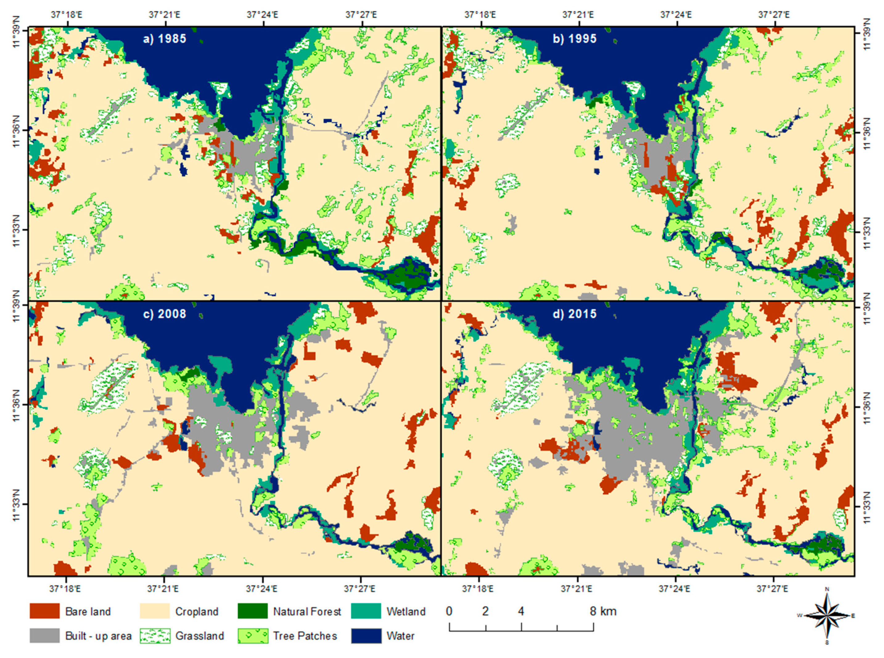
3.3. Land Use/Land Cover (LULC) Changes

Drastic changes took place in the past 30 years in Bahir Dar, resulting in an increase of bare land, built-up areas, and tree patches at the expense of cropland, natural forest, grassland, and wetland (

Table 6. Results of LULC changes between different periods in hectare (ha) and percentage in percentage (%).

	LULC Changes between Periods
	1985–1995		1995–2008		2008–2015		1985–2015
LULC Class	Area (ha)	%	Area (ha)	%	Area (ha)	%	Area (ha)	%
Bare land	32.49	2.68	222.525	17.86	215.51	14.68	470.52	38.79
Cropland	667.62	2.53	–387.99	–1.44	–2062.85	–7.74	–1783.22	–6.76
Grassland	–335.88	–14.08	–1059.885	–51.71	–112.41	–11.36	–1508.18	–63.22
Built-up	87.89	9.33	1250.055	121.39	1021.91	44.82	2359.85	250.53
Natural Forest	–464.94	–70.21	–47.52	–24.09	–18.18	–12.14	–530.64	–80.13
Tree Patches	167.4	7.98	80.55	3.55	735.21	31.33	983.16	46.84
Water	–87.255	–1.75	–25.56	–0.52	254.75	5.24	141.93	2.85
Wetland	–67.32	–5.13	–32.175	–2.58	–33.93	–2.80	–133.43	–10.16

). The area covered with water remained almost constant during the whole study period. In 2015, built-up areas became the third most dominant land cover type with a proportion of 8.3% of the total area.

Certain trends were observed in the cropland class over the years. In 1995 its area peaked at 67.7% of the total area and then started decreasing. In 2015 its distribution dropped down to 61.5%.

During the first study period (1985–1995) natural forest drastically decreased by 70.2% (464.94 ha), followed by a reduction of grassland and wetland by 14.1% (335.88 ha) and 5.1% (67.32 ha), respectively. On the other hand, a slight increase of built-up areas (9.3%), tree patches (7.98%), bare land (2.7%), and cropland (2.5%) were observed.

Natural forest and wetland continued decreasing in the next period 1995–2008 by 24.1% and 2.6%, respectively. The highest decrease in 1995–2008 was detected in grassland, which was reduced by 1059.9 ha (51.7% of its 1995 area). On the contrary, the built-up class expanded from 1029.8 ha in 1995 to 2279.9 ha in 2008—resulting in a 121.4% increase. Tree patches and bare land continued increasing by 3.6% and 17.9%, respectively. At the end of the second study period (1995–2008), cropland decreased by 1.4% which could be explained by the increase in built-up area at the expense of other LULC classes. For instance, 47.5% of the built-up area in 2008 was converted from cropland.

During the third study period (2008–2015), cropland, grassland, natural forest, and wetland continued decreasing by 7.7%, 11.6%, 12.4%, and 2.8%, respectively. On the other hand, built-up area added 1021.91 ha of land, resulting in a 44.8% increase during this period.

Overall, the most significant change was observed in the built-up area which expanded by 250.5%, from 941.94 ha to 3301.79 ha (Table 6). Similarly, the tree patches class showed the second-highest level of growing by an increase of 983.16 ha (46.8%, compared with 1985). At the end of this study period, bare land increased by 470.52 ha (38.8%). Natural forest demonstrated the most significant negative change with a decrease of 80.1%.

Furthermore, during the 30-year period, grassland decreased by 63.2%, from 2385.72 ha to 877.55 ha. A negative trend was observed in the cropland class which slightly decreased by 1783.22 ha (6.8%), compared with that of 1985. Wetland decreased by 10.2% to an area of 1179.41 ha in 2015. Regarding changes in the water class, inundated lands were classified as water in the 2015 map which in turn lead to a slight increase of 141.93 ha of the class.

Through a change detection analysis, a conversion matrix was produced to display the conversions between different LULC classes in the study period (1985–2015) (

Table 7. Summary of LULC conversion matrix in ha from 1985 to 2015. ^a Row total sums the amount of land for each LULC types of the initial study year (1985); ^b column total sums the amount of land Table 2015. The bold diagonal values represent the area of each class that remains unchanged while the off diagonal values represent the change in area.

From	Bare Land	Cropland	Grassland	Built-Up	Natural Forest	Tree Patches	Wetland	Water	TOTAL (2015)b
To
Bare land	197.81	1260.68	90.37	15.34	7.44	103.07	2.66	6.25	1683.63
Cropland	716.56	20,769.16	1313.34	127.14	106.04	1045.32	327.93	173.10	24,578.60
Grassland	73.68	491.77	234.08	27.73	8.44	20.57	20.00	1.26	877.54
Built-up	150.98	1886.15	284.48	687.52	2.24	229.27	39.97	21.18	3301.79
Natural forest	0.00	0.00	0.00	0.62	102.34	1.74	3.72	23.16	131.58
Tree patches	62.51	1544.89	185.07	66.75	278.84	618.04	221.74	104.17	3082.00
Wetland	10.82	139.90	217.80	9.97	98.56	72.67	497.91	131.77	1179.40
Water	0.74	269.26	60.58	6.88	58.31	8.16	198.90	4513.63	5116.45
TOTAL (1985)a	1213.11	26361.81	2385.72	941.94	662.22	2098.85	1312.83	4974.52	39,951

). Although the conversion between the LULC classes varied substantially, 69% of the area remained unchanged during the study period in 1985–2015 while 31% was subjected to intensive change among the classes. Regarding their initial area, the top three LULC classes prone to major conversion were grassland, natural forest, and bare land with 90.19%, 84.6%, and 83.7%, respectively. Even though the cropland class experienced comparatively low change (21.2%), in absolute values it represented an area of 5592.65 ha or 45.4% of the total area that was changed between 1985 and 2015. Grassland represented only 17.4% of the total study area change and experienced the most dramatic change by 90.2%, compared with its initial area in 1985. This came as a result of the 63.2% decline in the area of grassland in 2015, compared with that of 1985. Therefore, from the total 2385.72 ha of grassland in 1985, only 234.08 ha remained unchanged. The conversion to cropland accounted for 55% of the total change in the grassland class. The second biggest change in the class was caused by conversion of 284.48 ha (11.9%) of grassland into built-up areas. On the other hand, according to the classification in 2015, 491.77 ha of cropland were either abandoned or left for restoration, thus, accounting for 56% of the overall grassland area in 2015. Natural forest was the class subjected to the second-highest conversion change. For instance, out of the 662.22 ha in 1985, only 102.34 ha remained unchanged and the remaining 84.6% were converted to other LULC classes. Out of the total area of 3082 ha of tree patches in 2015, 278.84 ha were fragmented natural forest and converted to tree patches. Additionally, 16% of the natural forest was converted to cropland, mostly along the Abay (Blue Nile) River on the eastern side of the city. The increase of 38.8% of bare land until 2015 was characterized by certain conversion patterns. In general, 83.7% of the bare land was subjected to change, comprising 1015.30 ha out of 1213.11 ha in 1985 that were converted to and from other LULC classes. Cropland was subjected to a 21.2% change in area compared to 1985, and it was primarily converted to built-up area (1886.15 ha), tree patches (1544.89 ha), and bare land (1260.68 ha). On the other hand, cropland replaced 1,313.34 ha of grassland and 1,045.32 ha of tree patches until 2015. Additionally, 327.93 ha of wetlands were converted to cropland.

The built-up class demonstrated certain patterns of change. For example, for the whole period 1985–2015, 1,886.15 ha of cropland were converted to built-up areas, which accounted for the biggest share of class conversion to built-up with 57% of the whole built-up area in 2015. The conversion from grassland to built-up area had the second biggest share with 284.48 ha turning into built-up area until 2015, followed by 229.27 ha of tree patches which were replaced by the built-up class. Even though natural forest experienced the highest negative change from all other classes with a decline of 80.13% and total area change of 84.6%, the conversion to built-up area accounted for only 2.24 ha (0.07%) of the total 559.88 ha of natural forest, which were converted to other classes. Nevertheless, 278.84 ha, which accounted for 42% of the natural forest in 1985, were already converted to tree patches in the classification of the 2015 image. The built-up class demonstrated the highest growth by newly adding 2359.85 ha of area or 250.5% of increase during the period analyzed in the whole study area. The major conversions were from cropland (1886.15 ha), grassland (284.48 ha), tree patches (229.27 ha), and bare land (150.98 ha).

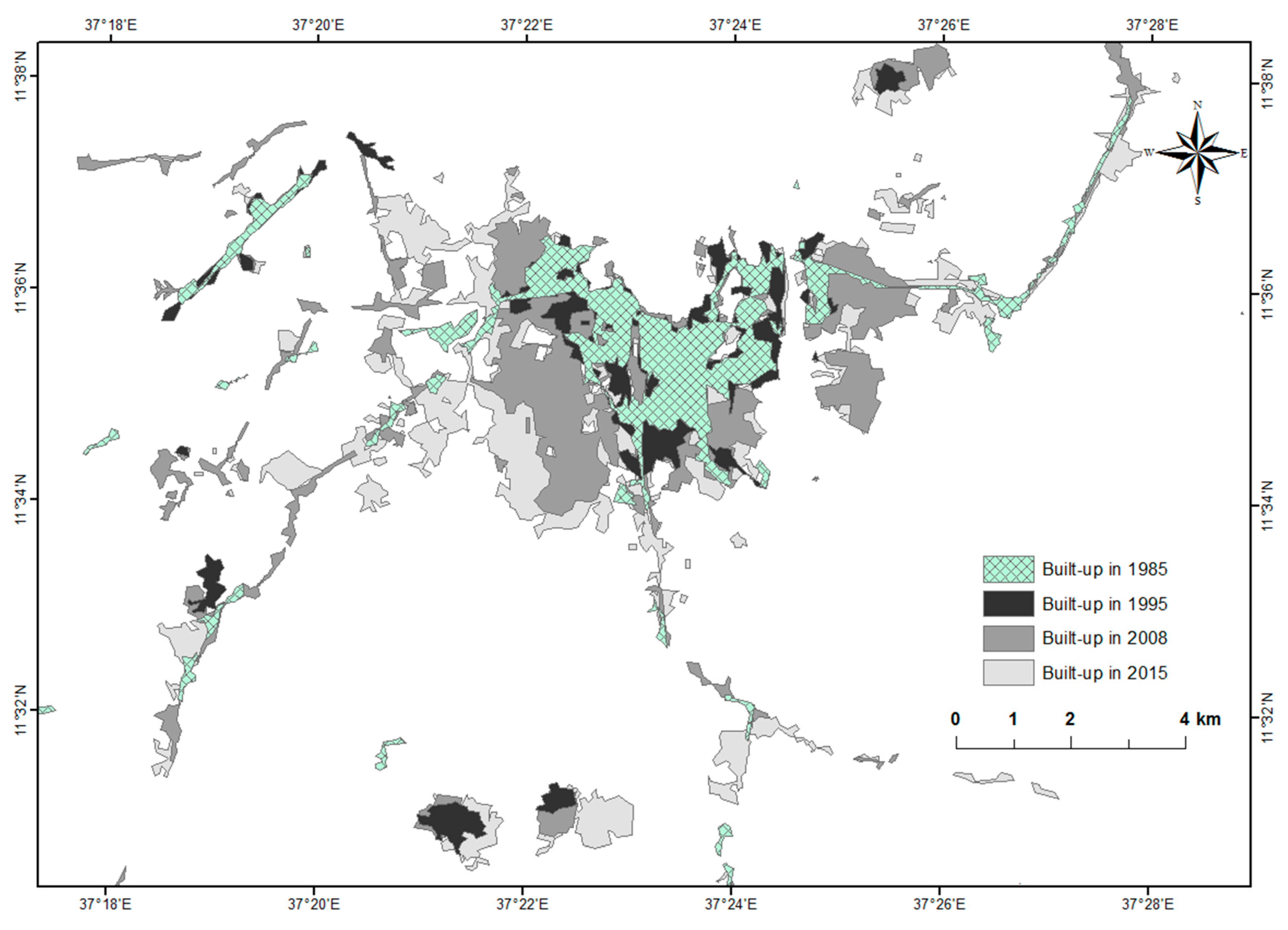
3.4. Expansion of Built-Up Area

The total built-up area calculated within the administrative boundaries of Bahir Dar was estimated at 941.94 ha, 1029.83 ha, 2274.88 ha, and 3301.79 ha in 1985, 1995, 2008, and 2015, respectively. The overall change between the periods 1985–1995, 1995–2008, 2008–2015, and 1985–2015 were 9.3%, 121.4%, 44.8%, and 250.5%, respectively.

The city expanded in all directions throughout the years, except to the north where Lake Tana was a natural barrier for urban growth (Figure 5). The city’s growth in the west is characterized by squatting, the Ginbot Haya airport and the hospital street. The expansion on the east is mainly related to stone quarries in the area and the presence of the Blue Nile (Abay) River, which provides easy access to water. Moreover, a major road which connects Addis Ababa and Gonder city passes through the eastern part of the city and significantly contributed to the expansion in the east.

4. Discussion

Monitoring of urban LULC changes provides critical inputs to evaluate complex causes and responses in order to project future trends better [2,9], and it is a prerequisite for making effective management plans [15]. Spatial urban LULC distribution and monitoring of growth patterns were conducted in rapidly growing Bahir Dar of northwestern Ethiopia by using satellite images of Landsat TM (1985, 1995, and 2008), and OLI (2015), and by employing object-based image analysis. All classified maps demonstrated an accuracy higher than the recommended target of 85%, which justified the degree of certainty to proceed with the next phase of the analysis [50].

The change analysis of 30 years (1985–2015) revealed that grassland and natural forest experienced the greatest reduction in terms of their area cover. The grassland was mainly converted to cropland and built-up area. The natural forest decreased mainly as a result of conversion to tree patches and cropland. Such trends of intensive changes in these LULC types are consistent with numerous studies in Ethiopia and elsewhere [29,54,55,56].

The analysis also revealed a general increase of the built-up area at the expense of cropland, grassland, tree patches, and bare land. This is in line with the outcomes of Lambin et al. [57], Xiao et al. [58], Aguayo et al. [58], Araya and Cabral [58], Forkuor and Cofie [58], and Mohan [59] who reported also a general decrease in the distribution of agricultural lands, due to an increase in built-up areas. For instance, Forkuor and Cofie [58] conducted a three-step study (1974, 1986, and 2000) on the land use and land cover dynamics in Freetown, the capital city of Sierra Leone, and evaluated the effects on urban and peri-urban agriculture. They observed similar conversion trends to the ones in Bahir Dar, where major changes occurred between agricultural lands, grasslands, evergreen forest, built-up areas, and bare land. The built-up area in Freetown increased by 140% between 1974 and 2000, mainly at the expense of cropland at the urban fringe. In total, about 27% (882 ha) of the cropland class was converted to residential areas in the period 1986–2000. On the other hand, 14% of evergreen forest was converted to cropland. Thus, Forkuor and Cofie [58] found a strong relationship between urbanization, agriculture conversion, and deforestation. Lambin et al. [57] discuss how urbanization in tropical regions affects the land in rural and peri-urban areas by consuming prime agricultural lands for residential purposes. Araya and Cabral [60] discovered that urban expansion often entails abandonment of agricultural lands and forest degradation, both of which substantially influence ecosystems. They found that urban areas in Setúbal and Sesimbra, Portugal increased by 91.11% for the period 1990–2006. Aguayo [61] also observed a similar dynamic between urban growth and cropland in Los Ángeles, Chile. Their results illustrated an increase of 65.5% of the constructed urban surface between 1978 and 1992, spreading urban use over 533.3 ha of former cropland. In their study, Miohan et al. [59] observed an identical trend where the increase of built-up area in Delhi, India was mainly caused by conversion from agricultural and waste lands. Xiao et al. [62] reported urban expansion of 15,919 ha at an average annual rate of 240 ha/year between 1934 and 2001 in Shijiazhuang, China. According to their study, urban regions are substantially expanding, croplands are shrinking, and windbreak trees and orchard are cleared.

In contrast to our finding, Mundia and Aniya [63] found that while the built-up area in Nairobi, Kenya expanded by 338% (4700 ha) between 1976 and 2000, cropland also increased by 78% at the expense of natural forest. Despite the difference in the cropland areas between both studies, a similarity was found where the natural forest area decreased by 77% and 80% in both Nairobi and Bahir Dar, respectively.

5. Conclusions

The study aimed to analyze LULC changes over a period of 30 years (1985–2015) in Bahir Dar, one of the rapidly growing cities in Ethiopia. The changes were analyzed and examined by object-based classification of multi-temporal remotely sensed images from four reference years followed by post classification comparisons using recent advancements of remote sensing (RS) and GIS technologies. These are vital technologies for continuous monitoring of urban LULC changes at varied spatial and temporal scales, which are otherwise not possible to attempt through simpler ground-based inventory methods. The framed approach used in this research is a good example of how to assess and monitor urban growth in developing countries like Ethiopia, by combining RS and GIS technologies. It enables a more efficient way of analysis. The generated datasets can be further used as an instrument for various applications, such as urban land use planning processes.

The quantitative change results revealed that built-up area was increasing while cropland, natural forest, and grassland were declining in Bahir Dar. A further focus was given to the temporal and spatial expansion of built-up area, and the consequences on the present state of the land cover. As a result, it was observed that the city has expanded considerably in all directions, except to the north where Lake Tana has naturally constrained urban growth. The urban growth patterns, which have been identified in this study show alarming trend of rapid urbanization of the city, which could severely impact the ecosystems and biodiversity around Lake Tana if appropriate measures are not taken in time to meet the growing demand of citizens. As the city is gradually expanding, three satellite towns, namely Zegie, Tis Abay, and Meshenti, which are already part of the Bahir Dar Special Zone, could become significant drivers of urban growth and attract further development in the future.

Further investigations about the drivers and implication of changes, as well as future effects of urban growth by developing a model would be helpful. As urban growth patterns substantially influence the nature and ecosystems, such a model could be used to illustrate future directions of development of Bahir Dar City. It can also provide an alternative outlook for addressing planning problems and formulating future management strategies in line with the sustainable development goals.

References

1. Lopez, J.M.R.; Heider, K.; Scheffran, J. Frontiers of urbanization: Identifying and explaining urbanization hot spots in the south of Mexico City using human and remote sensing. Appl. Geogr. 2017, 79, 1–10. [Google Scholar] [CrossRef]
2. Rebelo, A.G.; Holmes, P.M.; Dorse, C.; Wood, J. Impacts of urbanization in a biodiversity hotspot: Conservation challenges in Metropolitan Cape Town. S. Afr. J. Bot. 2011, 77, 20–35. [Google Scholar] [CrossRef] [Green Version]
3. Song, W.; Deng, X. Effects of Urbanization-Induced Cultivated Land Loss on Ecosystem Services in the North China Plain. Energies 2015, 8, 5678–5693. [Google Scholar] [CrossRef]
4. Ahrens, A.; Lyons, S. Changes in Land Cover and Urban Sprawl in Ireland From a Comparative Perspective Over 1990–2012. Land 2019, 8, 16. [Google Scholar] [CrossRef] [Green Version]
5. Mather, A.; Hancox, D.; Riginos, C. Urban development explains reduced genetic diversity in a narrow range endemic freshwater fish. Conserv. Genet. 2015, 16, 625–634. [Google Scholar] [CrossRef]
6. Schneider, A. Monitoring land cover change in urban and peri-urban areas using dense time stacks of Landsat satellite data and a data mining approach. Remote Sens. Environ. 2012, 124, 689–704. [Google Scholar] [CrossRef]
7. Lemonsu, A.; Viguié, V.; Daniel, M.; Masson, V. Vulnerability to heat waves: Impact of urban expansion scenarios on urban heat island and heat stress in Paris (France). Urban Clim. 2015, 14, 586–605. [Google Scholar] [CrossRef]
8. Schneider, A.; Friedl, M.A.; Potere, D. A new map of global urban extent from MODIS satellite data. Environ. Res. Lett. 2009, 4, 44003. [Google Scholar] [CrossRef] [Green Version]
9. Lambin, E.F.; Turner, B.L.; Geist, H.J.; Agbola, S.B.; Angelsen, A.; Bruce, J.W.; Coomes, O.T.; Dirzo, R.; Fischer, G.; Folke, C.; et al. The causes of land-use and land-cover change: Moving beyond the myths. Glob. Environ. Chang. 2001, 11, 261–269. [Google Scholar] [CrossRef]
10. United Nations Country Team Ethiopia. Assessing Progress Towards the Millenium Development Goals. Ethiopia MDGs Report 2012; Ministry of Finance and Economic Development: Addis Ababa, Ethiopia, 2012. [Google Scholar]
11. Kindu, M.; Schneider, T.; Teketay, D.; Knoke, T. Drivers of land use/land cover changes in Munessa-Shashemene landscape of the south-central highlands of Ethiopia. Environ. Monit. Assess. 2015, 187, 452. [Google Scholar] [CrossRef] [PubMed]
12. Kindu, M.; Schneider, T.; Döllerer, M.; Teketay, D.; Knoke, T. Scenario modelling of land use/land cover changes in Munessa-Shashemene landscape of the Ethiopian highlands. Sci. Total Environ. 2018, 622–623, 534–546. [Google Scholar] [CrossRef] [PubMed]
13. Nigatu, W.; Dick, Ø.B.; Tveite, H. GIS based mapping of land cover changes utilizing multi-temporal remotely sensed image data in Lake Hawassa Watershed, Ethiopia. Environ. Monit. Assess. 2014, 186, 1765–1780. [Google Scholar] [CrossRef] [PubMed]
14. Fenta, A.A.; Yasuda, H.; Haregeweyn, N.; Belay, A.S.; Hadush, Z.; Gebremedhin, M.A.; Mekonnen, G. The dynamics of urban expansion and land use/land cover changes using remote sensing and spatial metrics: The case of Mekelle City of northern Ethiopia. Int. J. Remote Sens. 2017, 38, 4107–4129. [Google Scholar] [CrossRef]
15. Jat, M.K.; Garg, P.K.; Khare, D. Monitoring and modelling of urban sprawl using remote sensing and GIS techniques. Int. J. Appl. Earth Obs. Geoinf. 2008, 10, 26–43. [Google Scholar] [CrossRef]
16. Nguyen, T.A.; Le, P.M.T.; Pham, T.M.; Hoang, H.T.T.; Nguyen, M.Q.; Ta, H.Q.; Phung, H.T.M.; Le, H.T.T.; Hens, L. Toward a sustainable city of tomorrow: A hybrid Markov—Cellular Automata modeling for urban landscape evolution in the Hanoi city (Vietnam) during 1990–2030. Environ. Dev. Sustain. 2019, 21, 429–446. [Google Scholar] [CrossRef]
17. Liping, C.; Yujun, S.; Saeed, S. Monitoring and predicting land use and land cover changes using remote sensing and GIS techniques—A case study of a hilly area, Jiangle, China. PLoS ONE 2018, 13, e0200493. [Google Scholar] [CrossRef]
18. Avelar, S.; Zah, R.; Tavares-Corrêa, C. Linking socioeconomic classes and land cover data in Lima, Peru: Assessment through the application of remote sensing and GIS. Int. J. Appl. Earth Obs. Geoinf. 2009, 11, 27–37. [Google Scholar] [CrossRef]
19. Santos, R.G.; Sturaro, J.R.; Marques, M.L.; Faria, T.T.d. GIS Applied to the Mapping of Land Use, Land Cover and Vulnerability in the Outcrop Zone of the Guarani Aquifer System. Procedia Earth Planet. Sci. 2015, 15, 553–559. [Google Scholar] [CrossRef] [Green Version]
20. Whiteside, T.G.; Boggs, G.S.; Maier, S.W. Comparing object-based and pixel-based classifications for mapping savannas. Int. J. Appl. Earth Obs. Geoinf. 2011, 13, 884–893. [Google Scholar] [CrossRef]
21. Taubenböck, H.; Esch, T.; Felbier, A.; Wiesner, M.; Roth, A.; Dech, S. Monitoring urbanization in mega cities from space. Remote Sens. Environ. 2012, 117, 162–176. [Google Scholar] [CrossRef]
22. Ma, L.; Li, M.; Ma, X.; Cheng, L.; Du, P.; Liu, Y. A review of supervised object-based land-cover image classification. ISPRS J. Photogramm. Remote Sens. 2017, 130, 277–293. [Google Scholar] [CrossRef]
23. Baatz, M.; Schäpe, A. Multiresolution Segmentation: An optimization approach for high quality multi-scale image. In Angewandte Geographische Informationsverarbeitung XII: Beiträge Zum AGIT-Symposium Salzburg 2000; Strobl, J., Blaschke, T., Griesebner, G., Eds.; Herbert Wichmann Verlag: Heidelberg, Germany, 2000; pp. 12–23. ISBN 978-3879073498. [Google Scholar]
24. Blaschke, T. Object based image analysis for remote sensing. ISPRS J. Photogramm. Remote Sens. 2010, 65, 2–16. [Google Scholar] [CrossRef] [Green Version]
25. Blaschke, T.; Hay, G.J.; Kelly, M.; Lang, S.; Hofmann, P.; Addink, E.; Feitosa, R.Q.; van der Meer, F.; van der Werff, H.; van Coillie, F.; et al. Geographic Object-Based Image Analysis—Towards a new paradigm. ISPRS J. Photogramm. Remote Sens. 2014, 87, 180–191. [Google Scholar] [CrossRef] [PubMed] [Green Version]
26. Myint, S.W.; Gober, P.; Brazel, A.; Grossman-Clarke, S.; Weng, Q. Per-pixel vs. object-based classification of urban land cover extraction using high spatial resolution imagery. Remote Sens. Environ. 2011, 115, 1145–1161. [Google Scholar] [CrossRef]
27. Wang, W.; Li, W.; Zhang, C.; Zhang, W. Improving Object-Based Land Use/Cover Classification from Medium Resolution Imagery by Markov Chain Geostatistical Post-Classification. Land 2018, 7, 31. [Google Scholar] [CrossRef] [Green Version]
28. Dronova, I.; Gong, P.; Wang, L. Object-based analysis and change detection of major wetland cover types and their classification uncertainty during the low water period at Poyang Lake, China. Remote Sens. Environ. 2011, 115, 3220–3236. [Google Scholar] [CrossRef]
29. Kindu, M.; Schneider, T.; Teketay, D.; Knoke, T. Land Use/Land Cover Change Analysis Using Object-Based Classification Approach in Munessa-Shashemene Landscape of the Ethiopian Highlands. Remote Sens. 2013, 5, 2411–2435. [Google Scholar] [CrossRef] [Green Version]
30. Bahir Dar City Administration. Urban Expansion Initiative Program; Bahir Dar City Administration: Bahir Dar, Ethiopia, 2013.
31. United Nations, World Meteorological Organisation (UN WMO). World Weather Information Service. Available online: http://worldweather.wmo.int/en/city.html?cityId=164 (accessed on 29 September 2016).
32. Central Statistical Authority (CSA). Summary and Statistical Report of the 2007 Population and Housing Census; CSA: Addis Ababa, Ethiopia, 2007.
33. Food and Agriculture Organization of the United Nations (FAO). FRA 2000 on Definitions of Forest and Forest Change. Available online: http://www.fao.org/docrep/006/AD665E/ad665e03.htm#P199_9473 (accessed on 8 February 2017).
34. European Environmental Agency (EEA). Corine Land Cover Commission of the European Communities; EEA: Copenhagen, Danmark, 1995.
35. Trimble. eCognition Developer 9.2; Trimble Germany GmbH: Munich, Germany, 2016. [Google Scholar]
36. Rougier, S.; Puissant, A.; Stumpf, A.; Lachiche, N. Comparison of sampling strategies for object-based classification of urban vegetation from Very High Resolution satellite images. Int. J. Appl. Earth Obs. Geoinf. 2016, 51, 60–73. [Google Scholar] [CrossRef]
37. Duro, D.C.; Franklin, S.E.; Dubé, M.G. A comparison of pixel-based and object-based image analysis with selected machine learning algorithms for the classification of agricultural landscapes using SPOT-5 HRG imagery. Remote Sens. Environ. 2012, 118, 259–272. [Google Scholar] [CrossRef]
38. McFeeters, S.K. The use of the Normalized Difference Water Index (NDWI) in the delineation of open water features. Int. J. Remote Sens. 1996, 17, 1425–1432. [Google Scholar] [CrossRef]
39. As-syakur, A.R.; Adnyana, I.W.S.; Arthana, I.W.; Nuarsa, I.W. Enhanced Built-Up and Bareness Index (EBBI) for Mapping Built-Up and Bare Land in an Urban Area. Remote Sens. 2012, 4, 2957–2970. [Google Scholar] [CrossRef] [Green Version]
40. Zhao, H.; Chen, X. Use of Normalized Difference Bareness Index in Quickly Mapping Bare Areas from TM/ETM+. Int. Geosci. Remote Sens. Symp. 2005, 6, 1666–1668. [Google Scholar]
41. Kawamura, M.; Jayamanna, S.; Tsujiko, Y. Relation between social and environmental conditions in Colombo Sri Lanka and the urban index estimated by satellite remote sensing data. Int. Arch. Photogramm. Remote Sens. Spat. Inf. Sci. 1996, XXXI, 321–326. [Google Scholar]
42. Qian, Y.; Zhou, W.; Yan, J.; Li, W.; Han, L. Comparing Machine Learning Classifiers for Object-Based Land Cover Classification Using Very High Resolution Imagery. Remote Sens. 2015, 7, 153–168. [Google Scholar] [CrossRef]
43. Lillesand, T.M.; Kiefer, R.W.; Chipman, J.W. Remote Sensing and Image Interpretation, 6th ed.; John Wiley & Sons: Hoboken, NJ, USA, 2007; ISBN 978-0-470-05245-7. [Google Scholar]
44. Congalton, R.G. A review of assessing the accuracy of classifications of remotely sensed data. Remote Sens. Environ. 1991, 37, 35–46. [Google Scholar] [CrossRef]
45. American Society of Photogrammetry and Remote Sensing (ASPRS). ASPRS Guidelines. Vertical Accuracy Reporting for Lidar Data; ASPRS: Bethesda, MD, USA, 2004. [Google Scholar]
46. Congalton, R.G.; Green, K. Assessing the Accuracy of Remotely Sensed Data. Principles and Practices, 2nd ed.; CRC Press Taylor & Francis Group: Boca Raton, FL, USA, 2009; ISBN 978-1-4200-5512-2. [Google Scholar]
47. Girma, Y.; Terefe, H.; Pauleit, S.; Kindu, M. Urban green spaces supply in rapidly urbanizing countries: The case of Sebeta Town, Ethiopia. Remote Sens. Appl. 2019, 13, 138–149. [Google Scholar] [CrossRef]
48. Abera, D.; Kibret, K.; Beyene, S. Tempo-spatial land use/cover change in Zeway, Ketar and Bulbula sub-basins, Central Rift Valley of Ethiopia. Lakes Reserv. 2019, 24, 76–92. [Google Scholar] [CrossRef] [Green Version]
49. Demissie, F.; Yeshitila, K.; Kindu, M.; Schneider, T. Land use/Land cover changes and their causes in Libokemkem District of South Gonder, Ethiopia. Remote Sens. Appl. 2017, 8, 224–230. [Google Scholar] [CrossRef]
50. Foody, G.M. Status of land cover classification accuracy assessment. Remote Sens. Environ. 2002, 80, 185–201. [Google Scholar] [CrossRef]
51. Singh, A. Review Article: Digital change detection techniques using remotely-sensed data. Int. J. Remote Sens. 1989, 10, 989–1003. [Google Scholar] [CrossRef] [Green Version]
52. Lu, D.; Mausel, P.; Brondízio, E.; Moran, E. Change detection techniques. Int. J. Remote Sens. 2004, 25, 2365–2401. [Google Scholar] [CrossRef]
53. Foody, G.M. Monitoring the magnitude of land-cover change around the southern limits of the Sahara. Photogramm. Eng. Remote Sens. 2001, 67, 841–847. [Google Scholar]
54. Garedew, E.; Sandewall, M.; Söderberg, U.; Campbell, B.M. Land-Use and Land-Cover Dynamics in the Central Rift Valley of Ethiopia. Environ. Manag. 2009, 44, 683–694. [Google Scholar] [CrossRef] [PubMed]
55. Lambin, E.F.; Meyfroidt, P. Global land use change, economic globalization, and the looming land scarcity. Proc. Natl. Acad. Sci. USA 2011, 108, 3465–3472. [Google Scholar] [CrossRef] [PubMed] [Green Version]
56. Ariti, A.T.; van Vliet, J.; Verburg, P.H. Land-use and land-cover changes in the Central Rift Valley of Ethiopia: Assessment of perception and adaptation of stakeholders. Appl. Geogr. 2015, 65, 28–37. [Google Scholar] [CrossRef]
57. Lambin, E.F.; Geist, H.J.; Lepers, E. Dynamics of land-use and land -cover change in tropical regions. Annu. Rev. Environ. Resour. 2003, 28, 205–241. [Google Scholar] [CrossRef] [Green Version]
58. Forkuor, G.; Cofie, O. Dynamics of land-use and land-cover change in Freetown, Sierra Leone and its effects on urban and peri-urban agriculture—A remote sensing approach. Int. J. Remote Sens. 2011, 32, 1017–1037. [Google Scholar] [CrossRef]
59. Mohan, M.; Pathan, S.K.; Narendrareddy, K.; Kandya, A.; Pandey, S. Dynamics of Urbanization and Its Impact on Land-Use/Land-Cover: A Case Study of Megacity Delhi. J. Environ. Prot. 2011, 2, 1274–1283. [Google Scholar] [CrossRef] [Green Version]
60. Araya, Y.H.; Cabral, P. Analysis and Modeling of Urban Land Cover Change in Setúbal and Sesimbra, Portugal. Remote Sens. 2010, 2, 1549–1563. [Google Scholar] [CrossRef] [Green Version]
61. Aguayo, M.I.; Wiegand, T.; Azócar, G.D.; Wiegand, K.; Vega, C.C.E. Revealing the Driving Forces of Mid-Cities Urban Growth Patterns Using Spatial Modeling: A Case Study of Los Ángeles, Chile. Ecol. Soc. 2007, 12. [Google Scholar] [CrossRef]
62. Xiao, J.; Shen, Y.; Ge, J.; Tateishi, R.; Tang, C.; Liang, Y.; Huang, Z. Evaluating urban expansion and land use change in Shijiazhuang, China, by using GIS and remote sensing. Landsc. Urban Plan. 2006, 75, 69–80. [Google Scholar] [CrossRef]
63. Mundia, C.N.; Aniya, M. Analysis of land use/cover changes and urban expansion of Nairobi city using remote sensing and GIS. Int. J. Remote Sens. 2005, 26, 2831–2849. [Google Scholar] [CrossRef]
Figure 1. Location of the study area. Background is a Landsat 8 OLI image from 2015 with RGB (red, green, blue).
Ijgi 09 00548 g001
Figure 2. Part of Bahir Dar city shown in a high-resolution satellite image from 2015 (Source: Google Earth).
Ijgi 09 00548 g002
Figure 3. Flowchart of the image classification process.
Ijgi 09 00548 g003
Figure 4. Land use/land cover (LULC) map of the study area.
Ijgi 09 00548 g004
Figure 5. Horizontal expansion of Bahir Dar between 1985 and 2015.
Ijgi 09 00548 g005