1. Introduction
Indoor positioning systems (IPSs) are a reality and provide location information of devices and persons for different applications in the real world. With the appropriate technology, it is possible to locate products in a warehouse, firefighters in a burning building, medicines in a hospital, maintenance tools spread over a plant, and so forth [
1]. Moreover, with the ascending global need for smart devices and connected networks, indoor positioning becomes one of the principal enabling technologies for a great variety of services in the context of the Internet of Things (IoT) [
2].
Applications already well established as Google Maps, Waze, and Uber are also location-based services, except that they are used outdoors. In this case, the most widespread technology is the Global Navigation Satellite Systems (GNSS), which includes the Global Positioning System (GPS). Unfortunately, GNSS does not perform well indoors, as it needs, among other factors, direct line of sight to the satellites and the device whose location one wants to know [
3].
An indoor positioning system must take into account some factors whose effects compromise the accuracy when estimating the location. Lack of line of sight, the influence of obstacles and obstructions such as walls and human movement, multipath propagation, and interference noises are examples of factors that result in the low performance of the most commonly deployed solutions [
4].
Most of these systems use wireless technologies such as WiFi or Bluetooth due to a wide available and accessible infrastructure, which saves time and related costs of deployment [
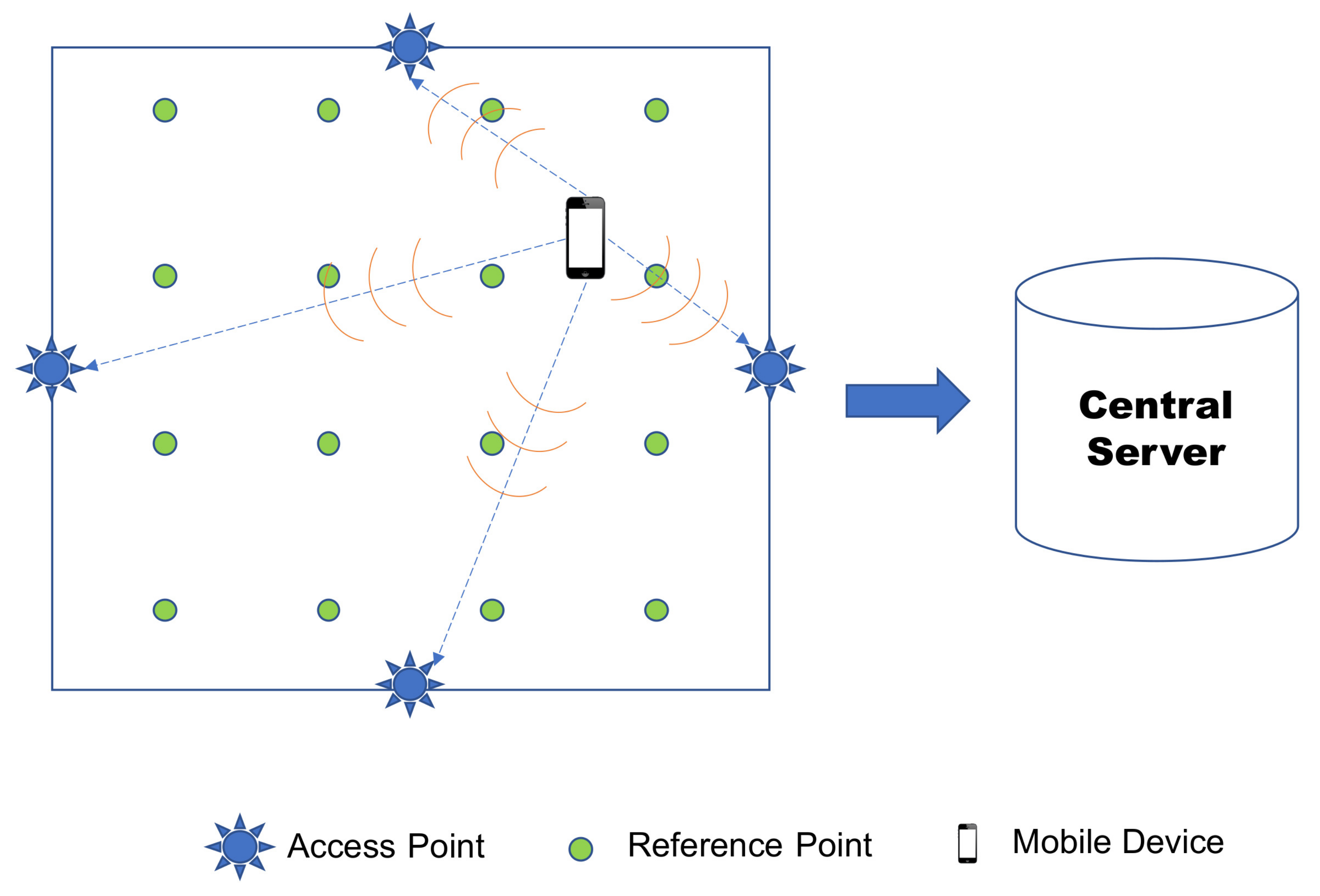
5]. A common architecture consists of mobile devices, access points (APs), and a central server. The main goal is to obtain location information of the mobile devices. To do this, the devices should transmit signals, whose power levels are captured by the access points which are spread over the environment. The power levels, well-known in the literature as Received Signal Strength (RSS), are passed on to the central server. After that, these data are processed using techniques and appropriate algorithms to determine the location of the devices.
Figure 1 better illustrates this situation.
There is a vast literature of positioning algorithms used for IPSs, which include deterministic and probabilistic methods. The first ones are quite common in fingerprinting-based localization, which basically consists of two main steps: an offline phase, in which RSS measurements (fingerprints) are previously collected in the environment; and an online phase, in which machine learning techniques and algorithms are used for the location estimation by a comparison between the offline database and the RSS data collected in real time. One of the first and most traditional systems is the RADAR [
6], which achieved a median error of 2–3 m. The second, probabilistic methods, are much more common in propagation model-based systems that take into account the random component inherent to the variability of RSS over the environment. In this case, the employed model is more likely to describe the indoor area reasonably. One advantage of this method is a better computational efficiency. A well-known probabilistic-based solution is the HORUS [
7], which achieved an error of approximately 2 m during 95% of the time for its particular testbed. Besides that, many systems provide hybrid solutions taking into account specificities of the indoor environment, seeking in general to improve accuracy. In this sense, IPS optimal design is also a hot research topic, since high localization performance can be achieved by means of a few infrastructure modifications [
8].
In this work, we propose a model and simulation based approach to optimize the deployment of the most relevant design factors that influence the accuracy of an IPS. In our work, they are restricted to the number of reference points (RPs), the number of samples collected per test, and the arrangement of the access points (APs) over the environment. Starting from the model parameters which describe the environment, we address the influencing factors and analyze their impact on the positioning error. Then, we propose a method to improve the system accuracy while keeping the number of RPs and the number of samples collected per test at minimal levels, followed by the achievement of an optimal AP configuration. This way, the desired accuracy can be reached by simply adjusting the values of the factors which compound the positioning system infrastructure.
The rest of the paper is organized as follows.
Section 2 reviews the literature.
Section 3 details the probabilistic-based model and its mathematical principles.
Section 4 presents the simulation environment, discusses the impact of relevant design factors on system accuracy, and describes a method to find an optimal combination of factors to achieve a required accuracy.
Section 5 presents a case study and an application based on a real-world dataset to validate the proposed method.
Section 6 concludes the paper.
2. Related Work
The related literature can be divided into two basic domains: the works which somewhat optimized the traditional probability-based positioning algorithms; and the works that developed methods to improve accuracy by either reducing the necessary number of APs or optimizing its placement over the indoor environment, which can be classified as general infrastructure components.
One of the first discussions about optimizing IPS design factors to improve accuracy was posed by the work of Kaemarungsi and Krishnamurthy [
9]. They used a probabilistic model to represent the RSS variation over the environment in fingerprinting-based systems. A framework was developed to analyze the influence of the number of APs, grid spacing between training points, and environment parameters on localization error. Although the fundamental theory and intuitions behind the design problem are carefully described, the authors neither propose nor apply a specific method to improve accuracy for real systems. Wendlandt et al. [
10] applied the concept of probability density functions to a Bluetooth-based IPS, but the work considered only a fixed scenario in regards to the number of RPs. Le Dortz et al. [
11] improved the results of classical positioning algorithms by using a hybrid probabilistic and nearest neighbor method. The work analyzed the impact on the system accuracy of the strongest signals from the APs, and the number of samples collected at the online phase. Nevertheless, the authors do not provide any general guideline for optmizing these influencing factors. Bisio et al. [
12] developed a smart probability-based method for IPSs, which considerably diminished the computational effort deployed for estimating the position when one RP only is considered for comparison with the traditional method. Li et al. [
13] proposed an enhanced probability positioning method by reducing the set of given reference points. Although it does reduce the localization error if compared to traditional methods, the results are demonstrated over a fixed and simulated scenario. Wu et al. [
14] provided a dynamic probabilistic approach, in which a guideline for deploying a reasonable number of APs is proposed given the size of the scenario. Despite the improvements, the arrangement of APs was not considered.
Concerning the optimization of infrastructure components, Hara and Fukumura [
15] proposed an efficient method to achieve a required localization accuracy with the deployment of a minimum number of access points. They use the maximum likelihood estimation to determine the location of targets and develop mathematical formulas that relate the variables involved in the optimization. Although they validate the proposed system experimentally, they do not take into account the impact of the arrangement of APs over the environment.
The previous consideration of finding an optimal AP placement is explored by Zhao et al. [
16] in which, given a fixed number of APs, a Differential Evolution algorithm is used to find the APs placement. Furthermore, the results were validated with model-based simulations and testbed experiments. Nevertheless, the authors do not elaborate on why the number of possible places for the APs to be allocated was considered fixed, which did not allow its associated impact—on both system accuracy and computational effort—to be addressed. He et al. [
17] used a genetic algorithm to determine both the minimum number of APs and the best arrangement of APs over an area to achieve the desired localization error. They simulate a fingerprinting-based IPS using the Nearest-Neighbors (NN) method for the location estimations. Although more complete from a simulation point of view, the work considered a fixed number for the RPs (or training points in this case) throughout all the simulations performed. Consequently, the impact of RPs on the system accuracy was not addressed.
From the 2010s on, most of the works have tried to apply efficient algorithms to optimize the placement of APs in an indoor area. Farkas et al. [
18] used an algorithm based on simulated annealing to find a minimum number of APs to achieve a required criterion of AP perceivability. They discretize the area in a reasonable number of points and indicate that the optimization problem is NP-hard, suggesting a method to approximate the global optimum solution. With
n possible AP location possibilities, they compare their obtained results for the time complexity—
—with the brute force algorithm—
. Despite the detailed approach, the work is geared towards localization with triangulation techniques. Aomumpai et al. [
19], on the other hand, worked with a path loss model considering obstructions and used the Binary Integer Linear Programming (BILP) method to optimize the number of APs. They compare their results with other approaches based on the average localization error achieved and do not mention the algorithm complexity issues. The scenarios and results were all obtained by simulation only.
Rajagopal et al. [
20] proposed a toolchain to optimize the number of beacons (APs) while keeping a sufficient signal coverage over the indoor plan. The metrics used to compare different configurations were an enhanced Geometric Dilution of Precision (GDOP) and the cumulative distribution function of the localization error. Several floor plans were used as scenarios and they demonstrated the improvement made by their method. Despite the promising results, the simulations were based on an ideal ray-tracing model, which perhaps might not be extended to more complex environments. Furthermore, there is not any mention relating to the time complexity of the proposed method. A similar work is presented by Sharma and Badarla [
21], except for the use of a Mixed Integer Linear Programming (MILP) approach and the extension for three dimensional (3D) indoor localization. In spite of the obtained improvements, a real testbed experiment for validation was not addressed. Jia et al. [
22] combined the previous works by proposing a technique to reduce the possible AP configurations for fingerprinting-based IPSs. They use a lognormal shadowing path loss model that includes walls and people attenuation, which brings more reality to the obtained results. Still, the work lacks considerations about the influence of the number of RPs (or training points simulated) and does not mention the time complexity of the proposed method. Palacios et al. [
23], on the other hand, proposed two algorithms, with proved effectiveness and scalability, which are robust to sparse environments in regards to the number of APs needed for computing the accuracy.
As we can see, many authors have tried to address the problem of optimizing the influencing factors that surround IPSs, mainly for improving localization accuracy. The majority of the research presented before relies on the construction of path loss models. However, a more complete performance analysis including the optimization of factors intrinsic to the deployed positioning algorithm, as well as the optimized arrangement of APs over an indoor site was not apparently done yet. In contrast, we propose an enhanced probability-based algorithm with both the number of RPs and the number of samples collected pert test optimized for a determined accuracy. Moreover, we use of the 95% interval of cumulative error distribution metric (instead of the classical average error) for more representative results. Finally, we analyze the time complexity of the proposed method and its associated impact on the design of efficient IPSs, which can give researchers some insights for improvements and future work. Hereupon, to the best of our knowledge, no work has either combined or addressed these listed design factors and optimized their values for achieving a required localization error.
3. Modeling of the Positioning System
In this section, we present the parameters of the log-distance path loss model, and how they contribute for the location estimation. We also introduce the Bayes theory and its mathematical properties applied to our problem of estimation, as well as the main references concerning the probability-based approach we use.
Although geometrical approaches for indoor positioning are vastly used, the high RSS variability is still a problem to handle. One reasonable choice is to use statistical models to deal with uncertainty [
24]. More specifically, the log-distance path loss model is a well established one to represent indoor signal propagation [
25], as shown in Equation (
1):
where
is a constant which represents the path loss in dB at a distance
used as a reference,
is the path loss exponent, and
is a normal random variable with zero mean and standard deviation
in dB, that is,
. All these parameters are determined for each environment and describe on average the distribution of RSS at a point distant
d from a transmitter. They are often obtained by collecting and processing RSS measurements with linear regression techniques or maximum likelihood estimation [
24]. The use of this probabilistic model for simulation purposes is convenient due to its reasonable approximation to real indoor positioning systems and the very efficient usage of computational effort in the process of localization.
For simplicity, we consider an IPS topology consisting of transmitters fixed over the room and receivers which one wants to locate. The first ones are known as APs, and the last ones are usually smart devices that can receive RSS information provided by the APs. This way, the goal is to simply collect and process RSS data to estimate the device location. The model presented before can be slightly modified to describe the distribution of RSS at each point over the area:
where
r is the perceived power in the receiver device and
is the AP transmission power. It is important to notice that
r is also a random variable, which can be represented by
, in which
is the expected value of the RSS for a point in the environment:
The equations listed above describe the distribution of RSS given a point distant
d from an AP, which is known in the literature as the likelihood function, whose probability density function (p.d.f) is given by:
where
l is such that
, with
l and
being the test point and the AP coordinates, respectively.
On the other hand, the main interest is to know the distribution of
l given the RSS information, which is obtained by the collected data. In this case, the posterior function contains the necessary information to estimate the location coordinate
l. According to Bayes’ rule:
where
is the prior function and
is a normalizing factor given by the total probability theorem:
Equation (
6) refers to the continuous case, in which
represents each possible coordinate uniformly distributed over the area. Although it is computationally unfeasible to calculate this integral analytically, an approximation to the discrete form can be done [
26]. That is, the area can be divided into many discrete coordinates as possible, treated here as the reference points (RPs). Likewise, the likelihood function is computed for each RP given. Thus, Equation (
5) can be rewritten as:
where
m is the number of RPs and
is the posterior function that relates the measure of RSS
r with location
, in which
.
The equations we have seen so far take into account one RSS sample from one AP only. However,
APs are considered in practical situations to improve accuracy, as it generates fewer ambiguities among the candidate RPs for the estimated location. In this case, the
n-dimensional RSS vector
is adopted instead of the one-dimensional
r. Another strategy to improve accuracy is to collect a sufficient number of RSS samples and take their mean for the estimation. According to the strong law of large numbers, the sample mean
tends to its true value
, as well as the Tchebycheff’s condition states that the variance of the estimator of the mean
tends to zero as
[
27]. Thereby, as variance diminishes, accuracy is improved due to fewer ambiguities in the estimation calculus.
Considering the multivariate Gaussian distribution [
28], the likelihood function already presented in Equation (
4) can be rewritten as:
where
is the covariance matrix, and
the vector with expected values for the RSS at location
. The exponential term of Equation (
8) is known, when its root is taken, as the Mahalanobis distance. However, we consider the RSS data provided by different APs as statistically independent, and a natural consequence is that the covariance matrix becomes diagonal. This way, the Mahalanobis distance reduces to the well-known Euclidean distance, becoming then:
Equation (
9) represents the likelihood function of a vector containing
n elements that correspond to the RSS from each of the
n APs. Next, the posterior function of Equation (
7) can be finally presented in its vectorial shape:
By knowing how to compute the probabilities for each RP, the final step is to find an estimator
for the position
ℓ. In our work, we use the maximum a posteriori estimate
, which simply gives the RP coordinate
that maximizes
in Equation (
10):
In other words, we seek for the RP coordinate
in regards to which the sum presented into the exponential term in Equation (
9) is minimized. This estimation is usually easy to determine [
29] as well as it needs less computational effort.
4. Analysis of the Impact of Design Factors on the System Accuracy via Simulation
In this section, we first describe the simulation environment used for analyzing the accuracy of using the probabilistic approach described previously by varying the main design factors of the positioning system. The localization error is calculated by taking the distance between the ground-truth position of each test point and the corresponding estimated location. Furthermore, the metric chosen for evaluating the overall performance is the 95% interval of cumulative error distribution.
The use of the error at 95% is particularly interesting because of its representative character along the entire area of study. The average error, in contrast, can instill a false notion that the error calculated is sufficiently small. An example of a concrete case occurs when most of the error is concentrated in a central part of the area, and the error at the borders is considerably large. This way, the average error is expected to represent the central area but not the entire room.
4.1. Construction of the Simulation Environment
The simulation environment is a tool to generate samples of RSS according to the log-distance path loss model. The extraction of environment parameters is the first step to build a consistent model. For WLAN-based systems, the technology often deployed is either WiFi or Bluetooth. In the next simulations for analysis, we chose the parameters based on some experiments of our research group, whose scenario is composed of Bluetooth Low Energy (BLE) devices, channel diversity, and high RSS variability. However, these values could be set to any reasonable interval, and are not constrained to the deployed technology [
30,
31,
32]. Specially, log-distance path loss models eventually fit better with BLE technology, although it can be also applied to WiFi or any other wireless technologies. The work presented by Zhao et al. [
33] highlights that RSS measurements relate better to range for BLE devices than for WiFi in the context of a log-distance path loss model. In order to be coherent to the results we shall verify further, the model parameters used for these preliminary simulations are very similar to the ones extracted from our real-world dataset, which is also BLE-based.
By using MLEs, the extracted parameters
,
and
used throughout this section in the next simulations are listed in
Table 1. Furthermore, the area is set to 100 m
and the transmitted power by the APs is set to −12 dBm.
From the point of view of the infrastructure components of the IPS, we consider, for simplicity, two-dimensional rectangular areas, and RPs uniformly distributed over the entire environment. The APs have also discrete and pre-determined possible locations, but not necessarily all of them are occupied. Next, the model parameters are specified. For more representative results, one often sets the parameters according to the propagation characteristics of the environment. The transmitted power
, in spite of being treated as a constant, is an important parameter for the accuracy computation. Generally, the more powerful an access point is, the more available APs for building the RSS vector we have, once the maximum range is relaxed, according to Equation (
2). Moreover, as we have more powerful APs, we naturally tend to need fewer of them to achieve a required accuracy. The value used in the next example is set to −12 dBm, which is typical for BLE devices. The other model parameters, represented by Equation (
1), are often obtained by means of regression techniques and maximum likelihood estimates (MLEs) from RSS databases. The parameter
is a constant dependent on the deployed radio-frequency hardware,
is the coefficient that represents how much the signal decays with distance, and
is a measurement of dispersion of RSS around its expected value. It is important to notice that a simulated scenario following the log-distance path loss model does not entirely represent the propagation features of an indoor environment. The parameters are highly dependent on the considered site, the hardware, and they can be even correlated, as pointed out by the work of Vallet García [
34]. However, although our simulation tool does not consider the variability (individually or jointly) of the model parameters, the simulated results are proved throughout the paper to be sufficiently representative and useful for the design of the type of IPS we propose.
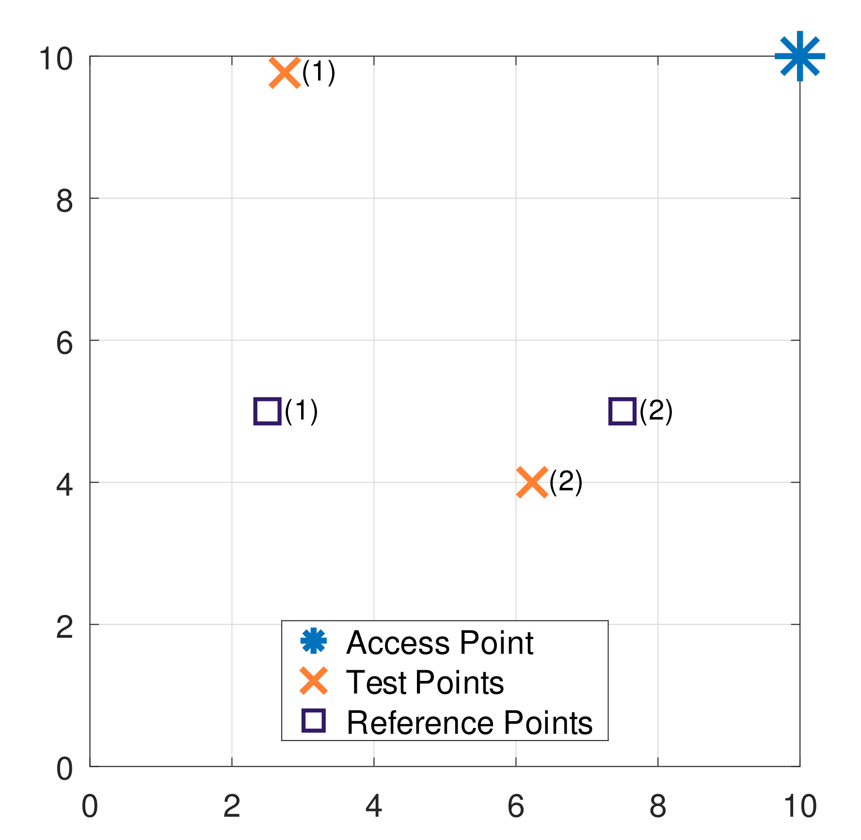
As for the simulation environment itself, we begin with a simple example with parameters that represent a possible indoor scenario. The fundamental point is to show how the estimation is computed in practice, thus we do not intend to extrapolate the obtained results for any existing type of environment. The scenario is built according to
Figure 2. There is one AP only and two RPs. In summary, the signal received by a device located in some part of the room is used to compute the probability for each represented RP. If the probability of one RP is higher than the other one, the first is chosen as the estimated location. This is how the MAP estimation works.
In terms of the simulation process, a signal with transmission power
is transmitted by the AP and values of RSS are registered into the variable
r described in Equation (
2) concerning test points (1) and (2). The random component extracted from the model
is used to generate the RSS measurements artificially with an adequate function from Octave [
35]. Furthermore, the test points are generated by the use of an inbuilt function that replicates uniform distributions. In the example, the test points coordinates in meters are
and
. The vectors
r generated are
(dBm) and
(dBm), which corresponds to the TPs (1) and (2), respectively. Next, these values are used to compute the posterior functions described in Equation (
10) for each RP. The results for
were
and
. For
, it followed that
and
. Finally, from Equation (
11), the estimated locations for the tests (1) and (2) were
and
, respectively. As expected, the estimations correspond to the RP locations given in
Figure 2. Indeed, it can be visually verified that
is closer to
whereas
is closer to
. Thus, for this specific example, the tests were classified correctly in terms of the RPs neighborhood, although the localization error can be still considered large.
Another way to observe how locations are estimated is to see the values of
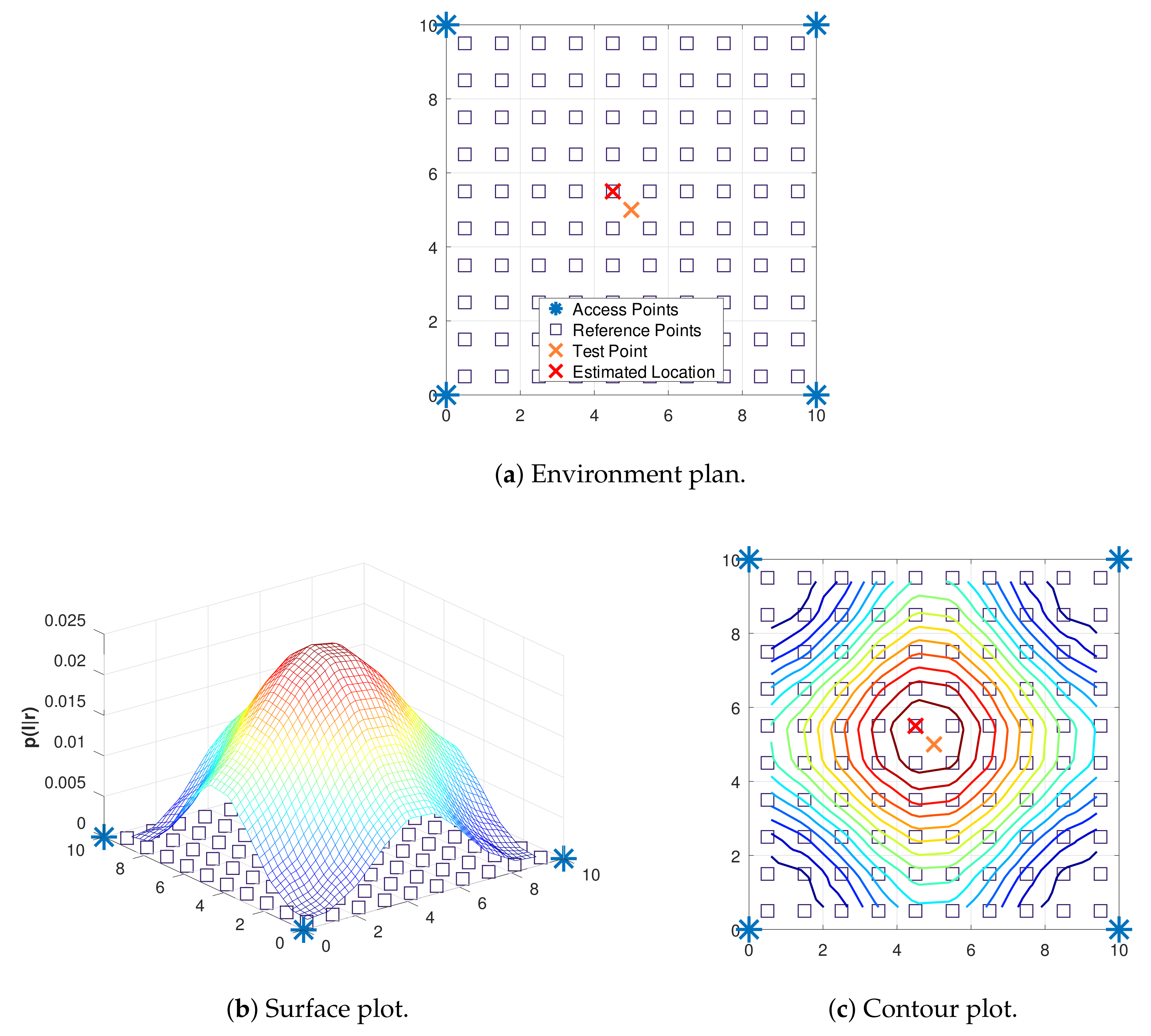
distributed over the environment. A new proposed scenario is described in
Figure 3a, in which only one test point is analyzed.
Figure 3b,c depict the probability that a RSS vector
is associated with each RP by means of surface and contour plots, respectively. As one can verify, the test point located at coordinates
is estimated as the RP with coordinates
, whose probability
associated is the maximum found among the other RPs.
4.2. Impact of Reference Points
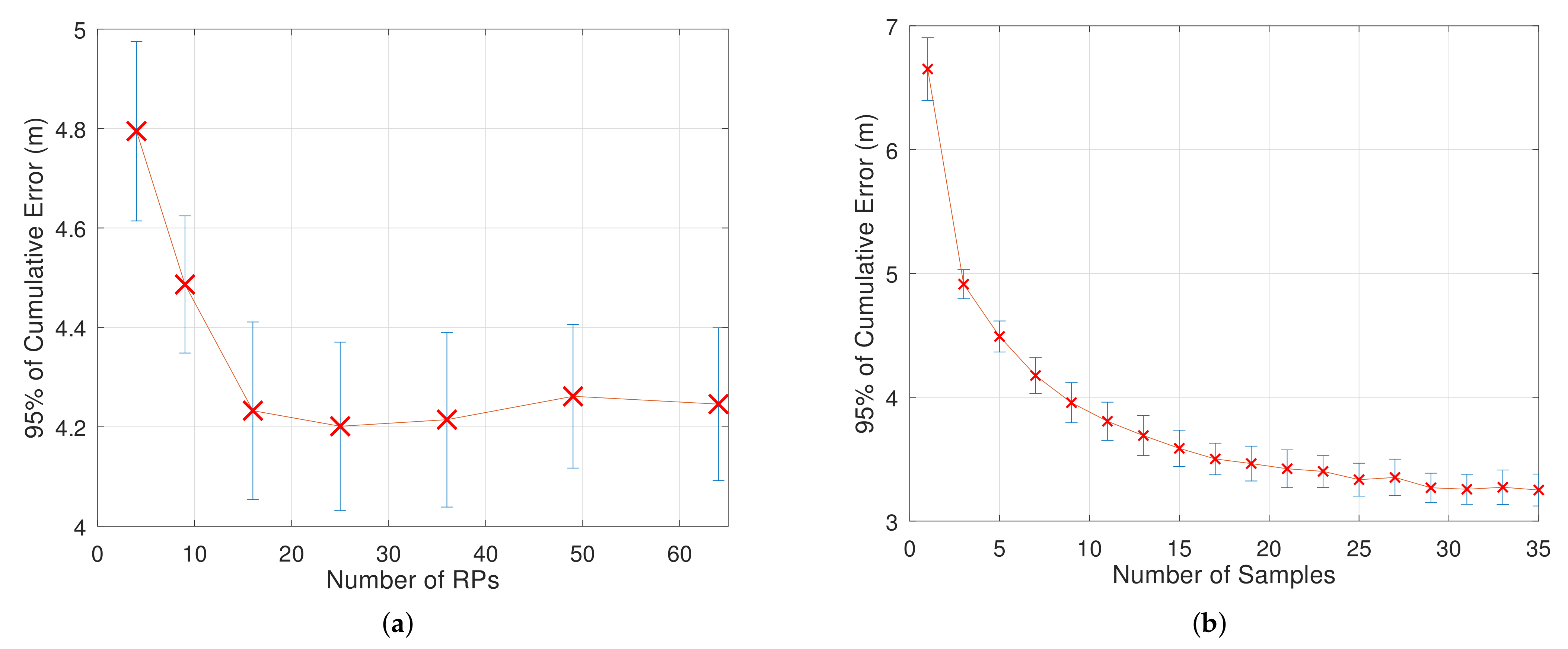
Figure 4a illustrates what occurs with accuracy in different scenarios concerning different number of RPs uniformly distributed. For the listed parameters in
Table 1, the curve has this descending pattern.
As one can observe, the error does not vary much from 16 RPs onwards. As the distance between closer RPs decreases to a certain point, the probabilistic-based positioning algorithm begins to have difficulty in estimating more precisely the RP closer to the true location of the test. Nevertheless, one cannot extrapolate these results for different combinations of model parameters, although we can assume that a limited set of RPs can surely have one element—approximately 25 according to
Figure 4a—that leads to the minimum localization error.
In terms of computational efficiency, the simulation is faster as the number of RPs decreases, once fewer comparisons are executed to cover all the requested tests.
4.3. Impact of Samples Collected per Test Point
Because of the high RSS variability, a technique usually employed for improving localization systems accuracy in practice consists of collecting more than one RSS sample during a determined time window [
36,
37]. This way, by taking the mean of these samples, for instance, the uncertainty in estimations is decreased, as mentioned before.
Figure 4b shows this situation, in which the error is decreased as the number of samples increases. It can be visually verified that the improvement in localization error is minimum from twenty-five samples per test on. In this case, the error decreasing rate also diminishes with the number of samples. These results indicate that one must choose a value for the “samples” variable that is optimal from the point of view of both accuracy and real-time positioning applications.
4.4. Impact of Access Points Placement
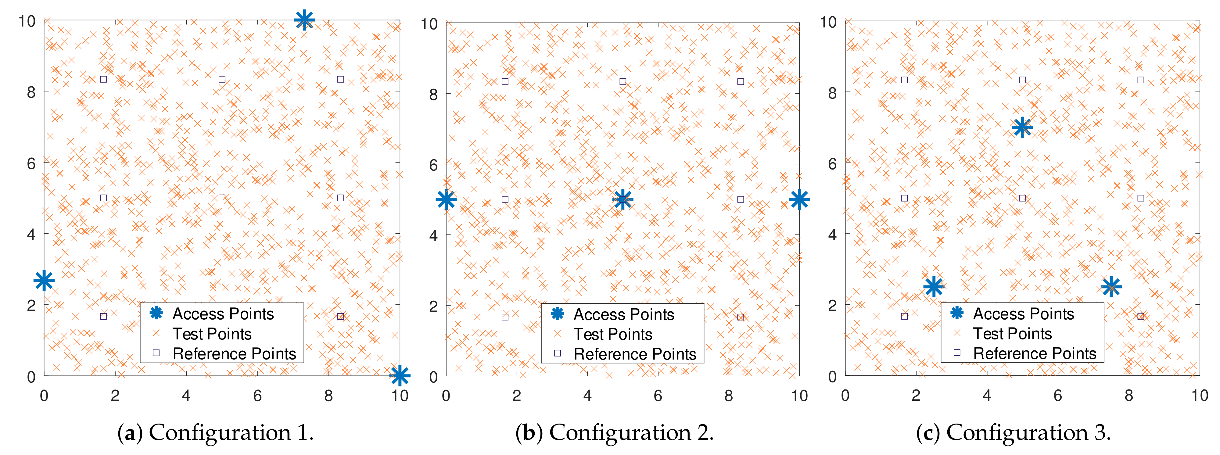
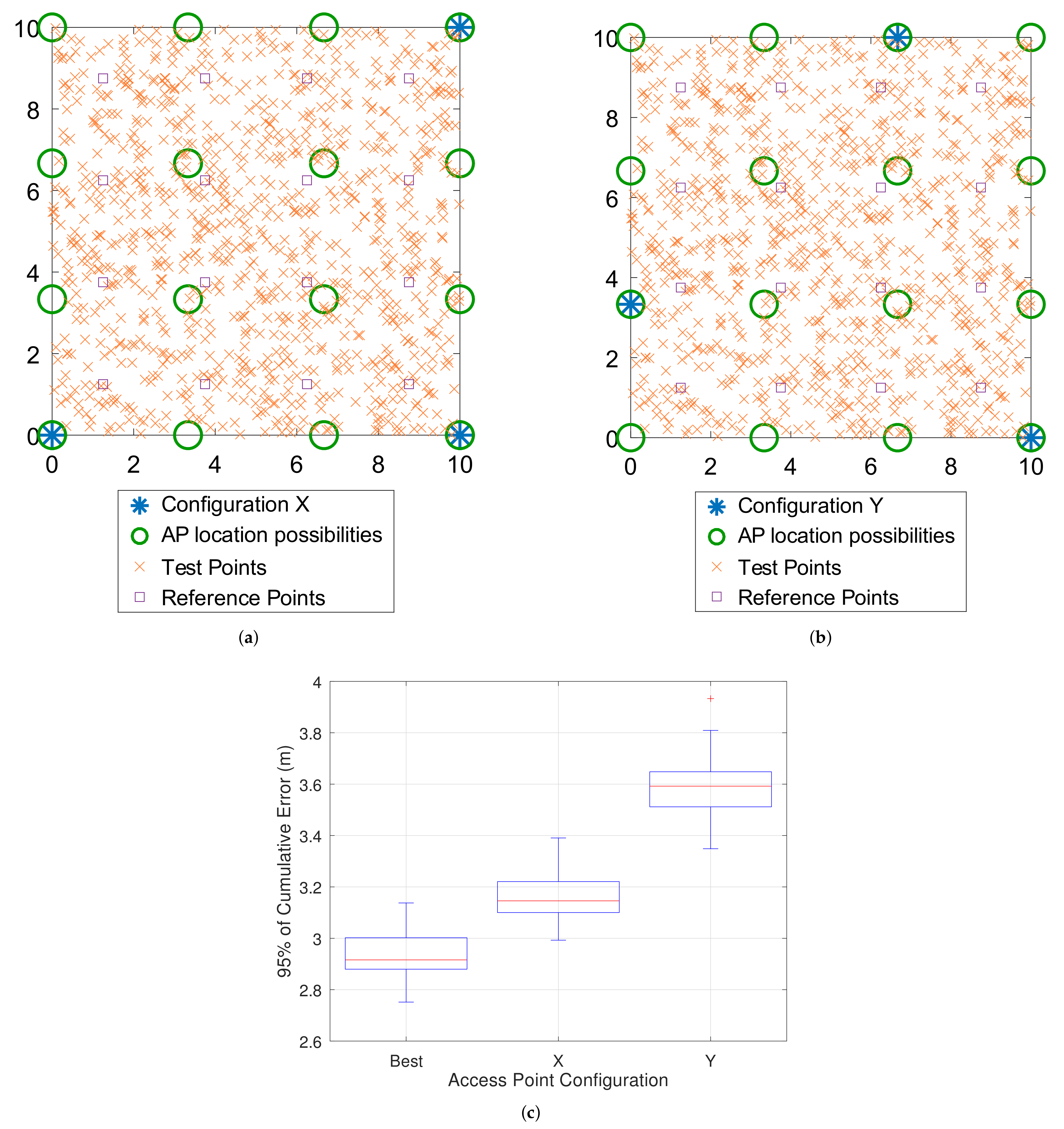
The APs placement is another factor that plays a relevant role when accuracy is a measure of performance. In what follows, three different AP configurations, represented by
Figure 5a–c, are proposed and their accuracy analyzed.
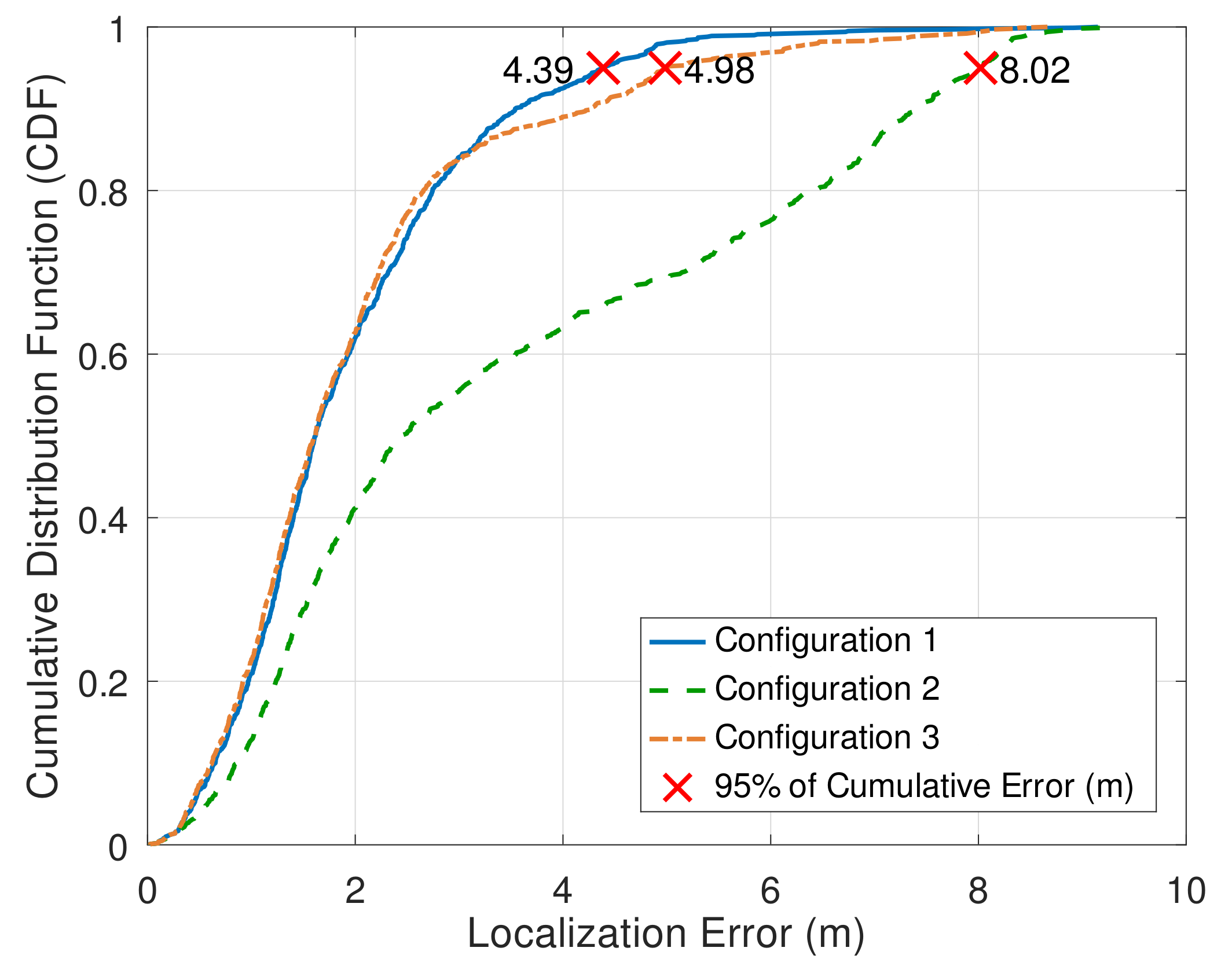
The simulation results are depicted in
Figure 6. It can be verified the difference in terms of localization error caused by the different AP configurations. The way the APs are arranged in the environment can generate more or fewer ambiguities when estimating the location of a test point. In this case, specifically, the triangular format of Configuration 1 is a much more accurate choice than the placement proposed by Configuration 2. On the other hand, Configuration 3 has an intermediate accuracy compared to the others. The results show the impact a simple arrangement of APs has on the accuracy of IPS. In principle, there is not an evident pattern that can produce smaller errors, which reinforces the need for simulating each given scenario extensively.
4.5. Method for the Best Design Choice
The analysis retracted previously indicates that it is possible to optimally combine the number of samples collected per test and the number of RPs to keep the localization error at a minimum level.
First of all, a reasonable number of APs is necessary to make the simulations feasible for analysis. In general, one has to guarantee that the RSS measurements from at least three APs are available for the location estimation [
38]. Regarding an area covered by the intersection of the achievable range R for each AP, it would be sufficient to collect RSS from three APs to get position information unambiguously. Consequently, at least four devices with a range of
a m each and located at the corners of a square of side
a are sufficient to cover most of the corresponding area of
m
. This is the premise we consider in this work, as the number of APs is fixed. The range, in turn, can be estimated given the environment parameters
,
and
, the AP transmission power
, and the sensitivity
S of the receiving device, after some manipulation of Equation (
2):
However, Equation (
12) does not consider the RSS variability represented by the parameter
for a more pessimistic scenario. In this sense, we estimate the maximum range from what we call the effective range
. It can be computed considering that the weakest signal, represented by
S, comes from a deviation of
around its expected value. We assume that there is an effective sensitivity
which determines the maximum distance a receiver device can be from the transmitter so that the RSS measurement is still reliable (95% of the time) from the point of view of a normal distribution. This way, Equation (
12) can be modified to express the effective range
:
From the results of Equation (
13), it is possible to allocate 4 APs at the corners of a square with an area of
to get reasonably accurate positioning information. This can be expanded for a general case of a rectangular plan with dimensions
a and
b. In this case, we adopt the convention to distribute the APs uniformly with the maximum distance among neighbors equals to their effective range
. The total number of APs can be expressed, thus, by:
Regarding the number of samples collected per test, there is a vast literature on indoor positioning addressing the benefits of a good choice for this factor. Faragher and Harle [
36] prove experimentally that taking the median or the mean of a batch of RSS measurements can significantly smooth the high variability of the data. This allows the system accuracy to be improved. Moreover, the authors demonstrated that a collection of 10 samples per test is sufficient, considering the beaconing rate of their employed devices (10 Hz) and the speed of the user as limiting factors. On the other hand, a lower bound of three samples per test in fingerprinting-based systems is proposed in the work of King et al. [
39] as a reliable number to achieve good accuracy results. The upper bound, however, must take into account the limiting factors already mentioned. If there is no real-time positioning requirement, 20 samples would be sufficient, considered here as the number of the collected fingerprints per point ideally proposed in [
39].
With the knowledge of how the factors relate to the localization error, a natural path is to find the best factor combination which achieves a determined accuracy given as input. In other words, a method that seeks to achieve the localization error requested with a minimum number of RPs and samples collected per test.
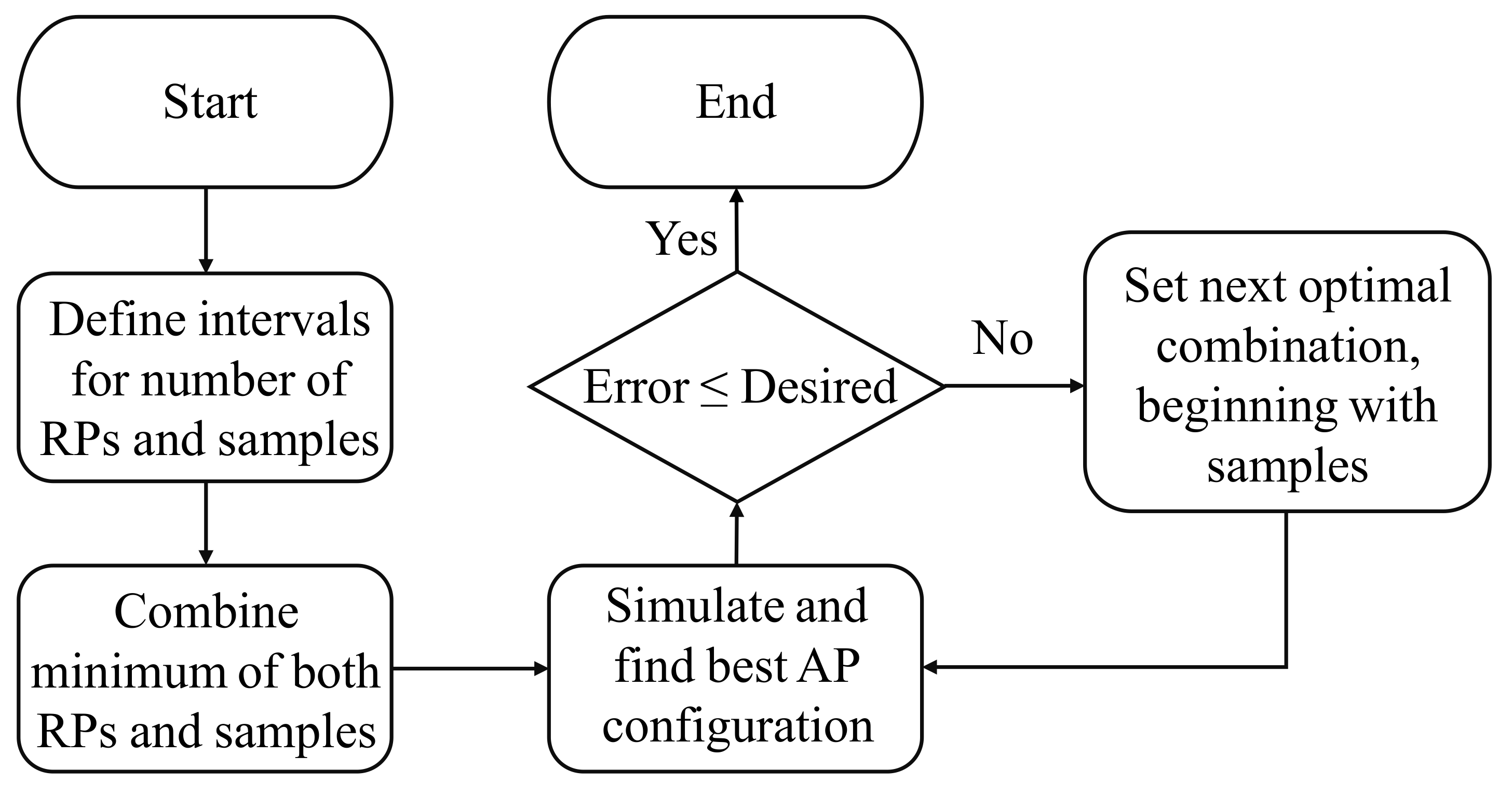
Our proposed method, in this case, consists of some basic steps and is represented by the flowchart depicted in
Figure 7. Given the environment lognormal path loss model parameters and its area, the number of APs, and the required positioning error, the proposed simulation sequence can be developed as follows:
- 1.
Establishment of limits for the number of samples and RPs. As we know that there is little gain in accuracy with considerably large values for these factors, superior limits can be set to restrict the possible combinations. For the number of samples, it depends on the application and the technical features of the employed devices . As a rule of thumb, a reasonable interval can be set up between 3 and 10 samples collected per test, but it is not mandatory. For the number of RPs, a low density regarding this factor can produce several poor localization accuracies. A high density, on the other hand, might not be necessary. Intuitively, the distance between neighboring RPs must reflect, to some degree, the required localization error based on the probabilistic model described. Adding to this, what is frequently observed in real IPSs, a reasonable interval would be 1–4 m.
- 2.
Establishment of the combination possibilities, keeping the number of RPs as small as possible. As we shall verify later, the number of RPs has a higher impact on the simulation run time than the number of samples collected per test. Thus, it should be the last variable to change (if necessary).
- 3.
Search for the best AP configuration. For “best” we mean the configuration with minimum localization error (95% of cumulative error for most of our simulations). Then, with combinations set up, the arrangement of APs becomes the variable of interest. For each combination of RPs and samples per test, the localization error is computed for every possible AP placement. If the result that gives the smallest error is either smaller than or equal to the required, then the best AP configuration was achieved. In other words, no more simulations are needed, once the influencing parameters involved are already optimized.
5. Performance Evaluation
In this section, we apply the method described before on a simulated case study, as well as we analyze the time complexity intrinsic to the proposed solution. Next, a BLE-based testbed experiment from a known dataset is used to validate our hypothesis that the method can improve the accuracy of a real IPS.
5.1. Preliminary Case Study
To evaluate the performance of our probabilistic-based approach, as well as our method for finding the best design choice, a preliminary case study is proposed. To simplify, the same environment parameters in
Table 1 is used. Furthermore, the sensitivity of the devices represented by each test point is set to −100 dBm.
Considering that the indoor area has 100 m, and that the expected indoor range for BLE devices is close to 10 m, three to four APs would be sufficient to provide a good coverage over the area. In this example, we choose three APs and 1000 test points for analysis. Furthermore, the desired localization error is set to 3.0 m, considering the 95% point of the cumulative distribution function for the error.
Concerning the set of possible combinations of the number of RPs and samples, the first is restricted to
, and the second to
. As can be seen, the total number of possibilities is 12. For each possible combination, a simulation is executed to find the AP placement which gives the minimum error. The optimization algorithm employed at this point is the brute force just to demonstrate the improvement in accuracy by the method described here. By taking the possibilities of AP placement over the environment as
uniformly distributed coordinates, it is possible to allocate and test
n APs given as input. The total possible configurations to analyze is the choice of
n out of
possibilities. To find a suitable value for
, one can think of the average distance among neighboring APs on a possible configuration. According to the experimental results reported by the work of Wu et al. [
14], there is no significant improvement in accuracy when adjacent BLE iBeacons are distant less than 3 m from each other. This, somewhat, gives us support to fix the value for the number of possible AP allocation spaces. In this case study,
is set to 16 and
n has the value of 3. Thus, the total number of combinations
is given by:
According to Equation (
15), the simulation environment is run 560 times and outputs the configuration with minimum localization error.
In
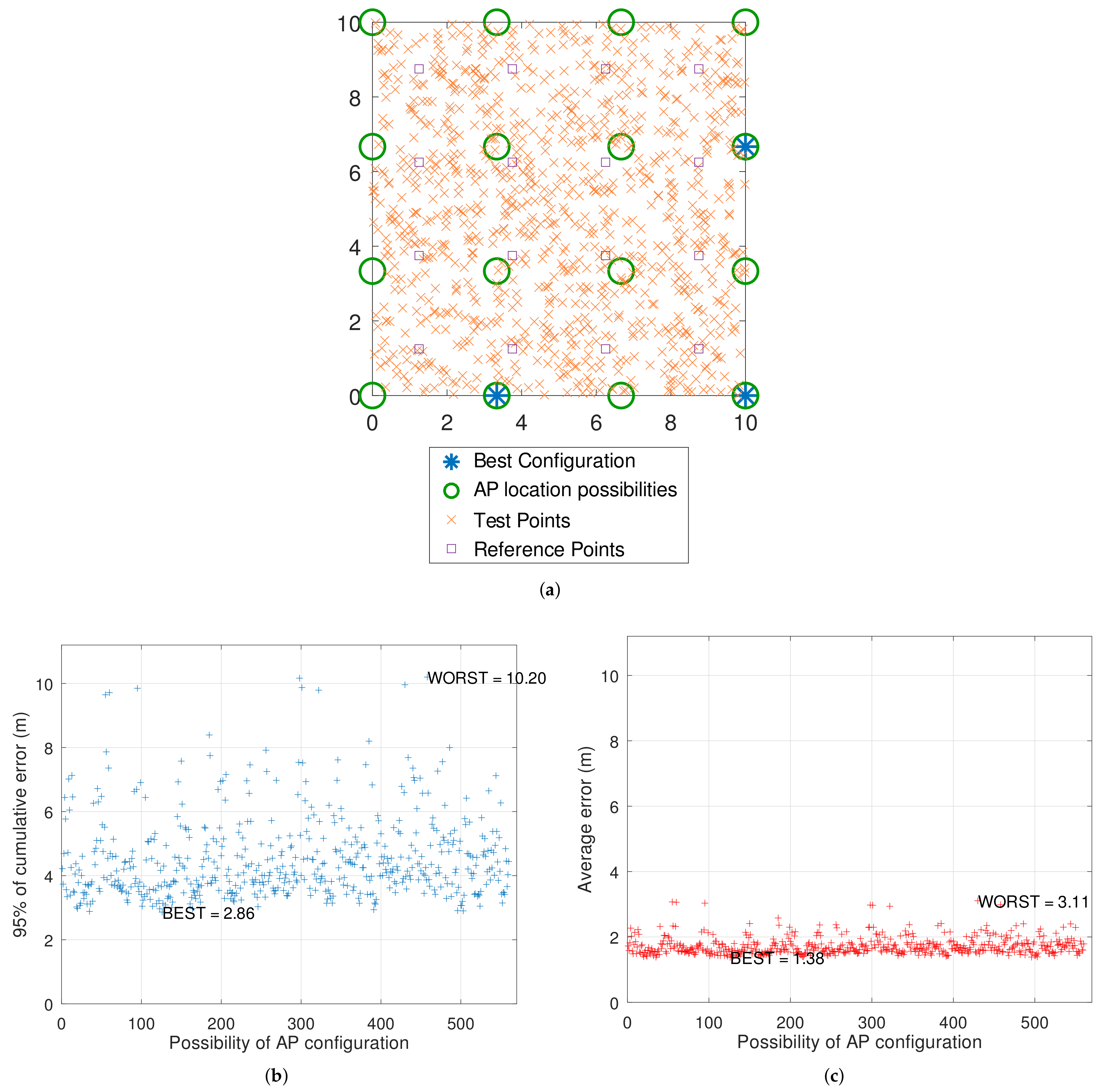
Table 2, the results for each parameter combination are shown. As one can verify, the combination which better fits the requirement of 3.0 m for the localization error is the one with 16 RPs and 10 samples per test, illustrated in
Figure 8a. A deeper analysis about this configuration is seen in
Figure 8b,c, in which different AP placements can produce even great differences in errors among each other. The “x” axis represents a map of indexes to the possible coordinates for the given scenario, generated by the function
nchoosek in Octave. At this point, it can be verified that the results from the 95% of cumulative errors were quite more dispersed than the results from the usual average. This shows that the first metric mentioned, besides promoting a better picture of the error distribution, can also provide a clearer contrast among the tested configurations.
In addition, it was observed that the configurations whose simulations processed only one sample per test gave very different AP placement patterns for the best accuracy found. Similar results were obtained when four RPs were used in simulations. On the other hand, from nine RPs and five samples per test onwards, all configurations which resulted in a minimum localization error have the same pattern of what is depicted in
Figure 8, being different from each other by a simple rotation of the room. One could argue, though, that this configuration is somewhat unexpected. The test points located at the upper left of the room, for instance, could have their estimations worsened due to the quite large distances among them and the APs. However, the results for the cumulative error show that the estimations are surprisingly accurate, which could be explained by the fact that the entire room reliably receives the transmitted signals by all the three deployed APs. Indeed, the worst possible scenario would be an AP and a test point located at opposite corners in regards to a diagonal of the squared room. In this case, the expected RSS would be then
dBm. Considering the variability represented by
, the 95% confidence interval for the RSS
r would be
, i.e.,
dBm
dBm, where the term
arises from the number of samples. This way, even the lower bound of
dBm is larger than the sensitivity S of
dBm, which is sufficient for an effective and reliable estimation all over this particular environment.
From another perspective, we can compare the localization error obtained with the configuration proposed in
Figure 8 to more intuitive configurations represented as X and Y in
Figure 9a,b, respectively. For each arrangement of APs, the simulation was run 100 times, and the results are presented in
Figure 9c. One cannotice the improvement in choosing the configuration obtained by using the optimization method. In this case, the results were, on average,
m for the 95% of cumulative error with a mean standard deviation of
m. That is, a localization error of
m, which constitutes a befitting value around the required of
m.
5.2. Time Complexity and Simulation Run Time Analysis
Although the method can achieve the goal of finding the combination with minimum localization error, there is a clear need to analyze the simulation time performance, mainly if we think of scaling the method for larger indoor areas. This includes, firstly, a general analysis about the time complexity regarding the variables given as inputs to the system for optimization.
For each location estimation, the computation for the error is proportional to both the number of samples collected and the number of RPs. The time complexity, thus, grows linearly as these two variables of interest increase. Asymptotically, the process of estimation is a linear time algorithm.
With respect to the number os possible AP allocation spaces , as it increases, the total possible configurations that must be run increases with , in which n is the number of APs. Once both and n should increase proportionally to the increase of the indoor area, the asymptotic behavior of the optimization algorithm is exponential. This is notably important for the method, as becomes the most restricting variable if we simply use a brute force algorithm for larger environments.
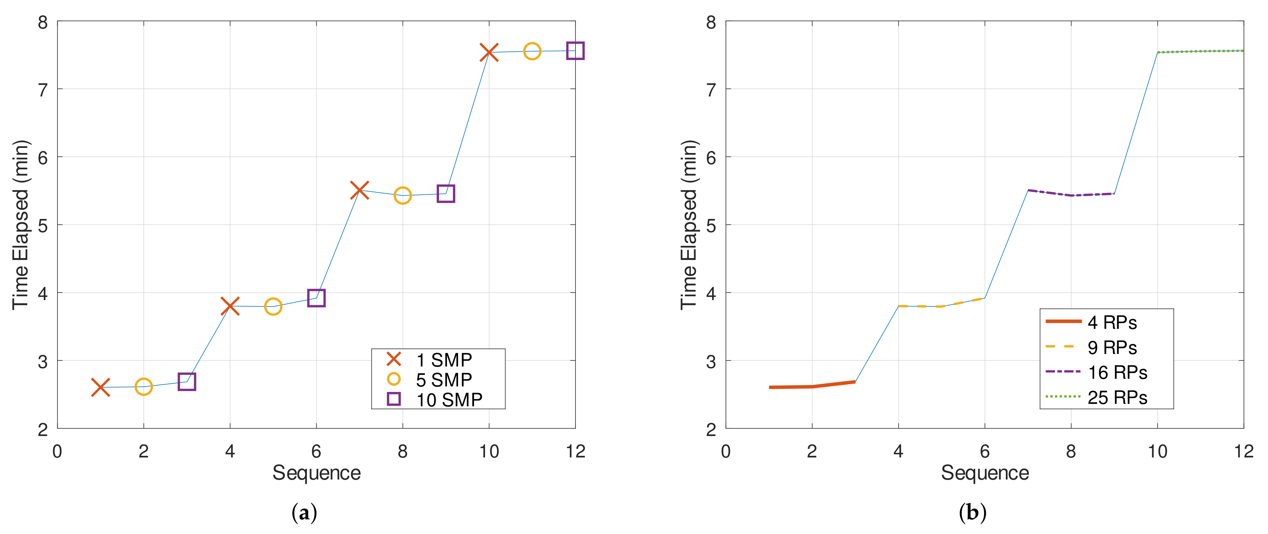
Next, one can verify the influence of each factor on the simulation run time in
Figure 10. The scenario is the same as the one provided in
Table 2. For this analysis, the simulation environment was developed using Octave-5.2.0 on a Sony Vaio laptop (Windows 10, 64-bit operating system, 2.70 GHz Intel i7-7500U Processor and 8 GB RAM). Furthermore, the time metric considered was the CPU time.
The influence of samples per test on the simulation time is negligible compared to the number of RPs. Indeed, the contribution from the number of samples is just a single calculation mean of RSS values for each test. On the other hand, the amount of additional time spent due to the number of RPs is considerably larger. This evidences the priority in changing the number of samples per test firstly, as it has little influence on the simulation run time.
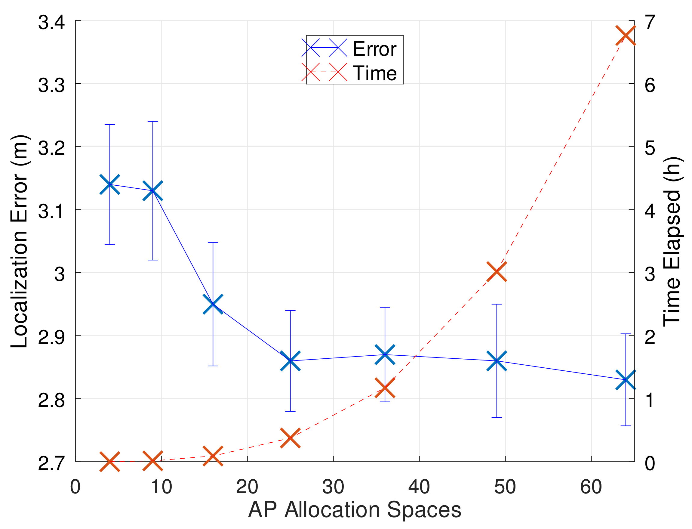
It is important to highlight that all of these previous simulations consider a fixed number of AP location possibilities. However, as commented before on the time complexity analysis, this variable also affects the simulation run time, as the more possible locations available to be allocated, the more configurations one has to simulate. For the same scenario depicted in
Figure 8a, simulations ranging from 4 to 64 AP allocation spaces were run, and some important results can be seen in
Table 3.
Although the localization error decreases as
increases, the total possible configurations that must be run increases with
. In this case, there has to be a trade-off between the goal of reducing localization error and the computational effort to be deployed.
Figure 11 better depicts this situation. As can be seen, the results make the method feasible for the relatively small area we consider of 100 m
. For larger areas, it is probably not practical to use the brute force algorithm due to the eventually high value obtained with the binomial relation between
and
n.
One way to set a fixed value for is to use the rule of thumb presented previously. The spacing of around 3 m among possible neighboring APs is equivalent to choose or , with spacings equal to 3.3 m and 2.5 m, respectively. These values follow what is verified graphically. From 25 possible AP allocation spaces onwards, the error is supposed to reach a threshold value around which there is no significant improvement. In this case, more allocation spaces possibilities would then overload the simulation unnecessarily.
5.3. Evaluation Using Real-World Data
Another question that may arise is the applicability of the proposed method on a real system. Although the simulation environment seen previously gives us some hints about the overall behavior of the system accuracy, it might not hold precisely in practice, especially if a practical requirement as the localization error is given as the objective function, or the stop criterion. Still, with adequate inputs, this type of previous simulation can anticipate overall trends or issues in real experimentation.
In this section, we divide our analysis into two parts: the use of the floor plan and the components (APs, RSS data for building the log-distance path loss model) of a real-world environment for the construction of one entirely simulated IPS; and the use of a set of figerprints from the dataset itself as test points to verify the localization error of our method in practice. After that, we compare the results obtained from the simulated environment with the obtained results by applying our method directly to the testbed experiment.
The database we use is presented in [
40] and described in detail in the work of Mendoza-Silva et al. [
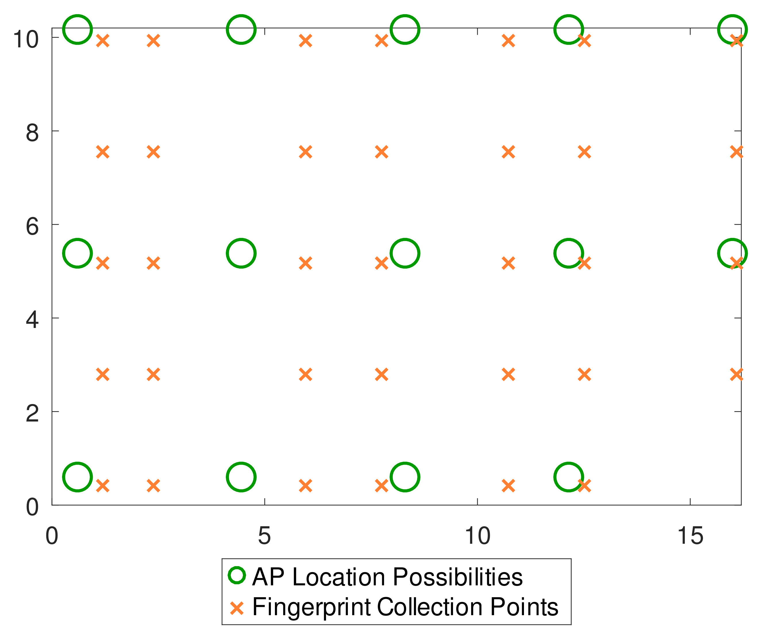
41], who are also the owners of the dataset. It is basically composed of the BLE RSS measurements collected on 34 points physically distributed over the Geotec room in two rounds, and each point has stored 26 fingerprints (13 for each round of collection performed) in regards to the 22 APs spread over the area. In our evaluation, we choose from the entire dataset the devices with transmission power of −12 dBm. This choice is made due to the availability of accuracy analysis provided by [
41] for this specific parameter. Thus, it is useful for us to compare the performance of our proposed method with what has already been presented in the literature regarding this dataset. We also choose the number of AP allocation spaces
to be 14 due to constraints of useful data for testing and spacing among the APs (in this case, 4 m). A simplified and adapted view of the scenario is depicted in
Figure 12.
The environment parameters were extracted by employing linear regression to fit the log-distance path loss model. The results are shown in
Table 4. It is important to address that the data used for the model fit were the fingerprints stored at the first round of RSS collection.
Firstly, a reliable number of APs must be initially set up. Being the receiver sensitivity
S equal to −100 dBm, it is possible to estimate the effective range
of the BLE devices according to Equation (
13). In this case, R
m. From Equation (
14), a reasonable number of APs would be around nine for the indoor area considered.
The simulated environment and the experiment are run by considering the same 34 test points coordinates. For the simulated environment, the test points are generated artificially according to the parameters of
Table 4. For the experiment itself, the data concerning the second round of collection of fingerprints were used for tests, i.e., they made the role of the test points for our system when we apply the method. This way, the subset of data used for fitting the parameters has no intersection with the subset of data for test points, except that they have the same coordinates.
The set of RPs is chosen to be
, due to a restricted spacing interval of 1.5–3.2 m, and the set of samples to
, to a fair comparison with the results reported in [
41]. Furthermore, in this regard, the metric used for the error was the 75th percentile of the cumulative distribution function to better compare the obtained results in this work with [
41].
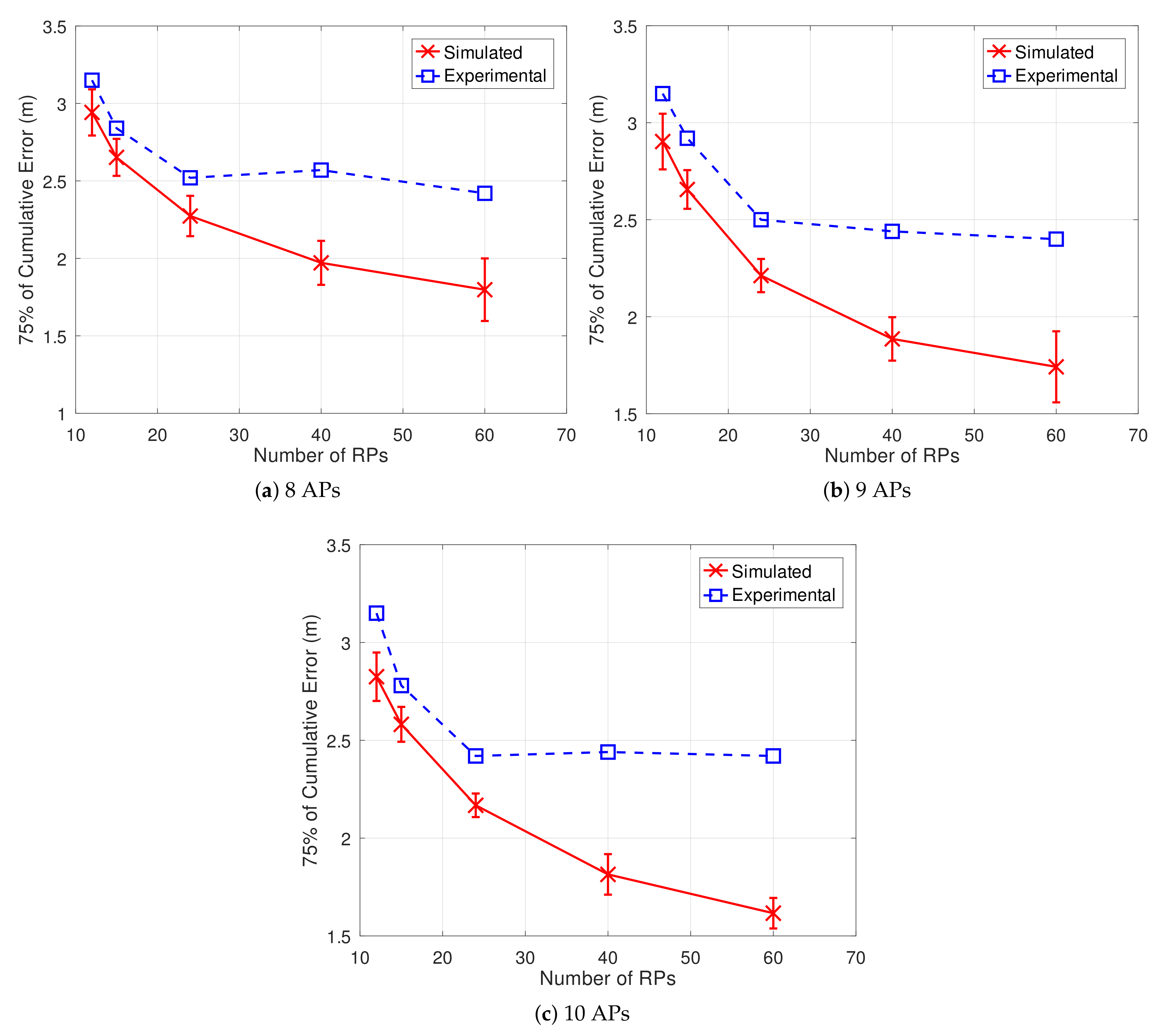
Table 5 shows the localization error obtained by the simulation and the real testbed experiment for each combination of RPs and samples, considering nine APs.
To fairly compare the simulation with the testbed experiment, the same process was also repeated to 8 and 10 APs. We use the Pearson correlation coefficient
as the metric for evaluation, whose results are described in
Table 6. The correlation is calculated based on the errors from each factor combination.
The obtained results show that there is, indeed, a strong correlation between the simulation and the practice. Moreover, this correlation is statistically significant, which is indicated by the very small p-values found. In other words, the trends observed by simulation are likely to be verified in practice. This way, a simulated setup with an optimal combination of RPs and samples would probably work satisfactorily in a real positioning system.
In
Figure 13, for each set of RPs allied with the best AP configuration found, the simulated scenario was run 100 times. It is possible to verify a similar decreasing rate tendency concerning the error between the simulation and the experiment. That similarity is stronger when nine APs are used, which is in accordance with the very high and significant value for the correlation reported.
As can be seen, an analysis of the trends regarding the error results obtained by simulation can serve as a reliable basis for the optimal design of the positioning system in practice. Although the errors found for the simulation and experiment differ substantially, the concrete contribution of an IPS simulated in advance is that an optimal combination of the number of samples per test and the number of RPs can be reasonably deployed in practice. Furthermore, the difference between simulation and practice is somewhat expected, due to the high loss verified in the dataset concerning the RSS values—which naturally worsens the performance of the algorithm.
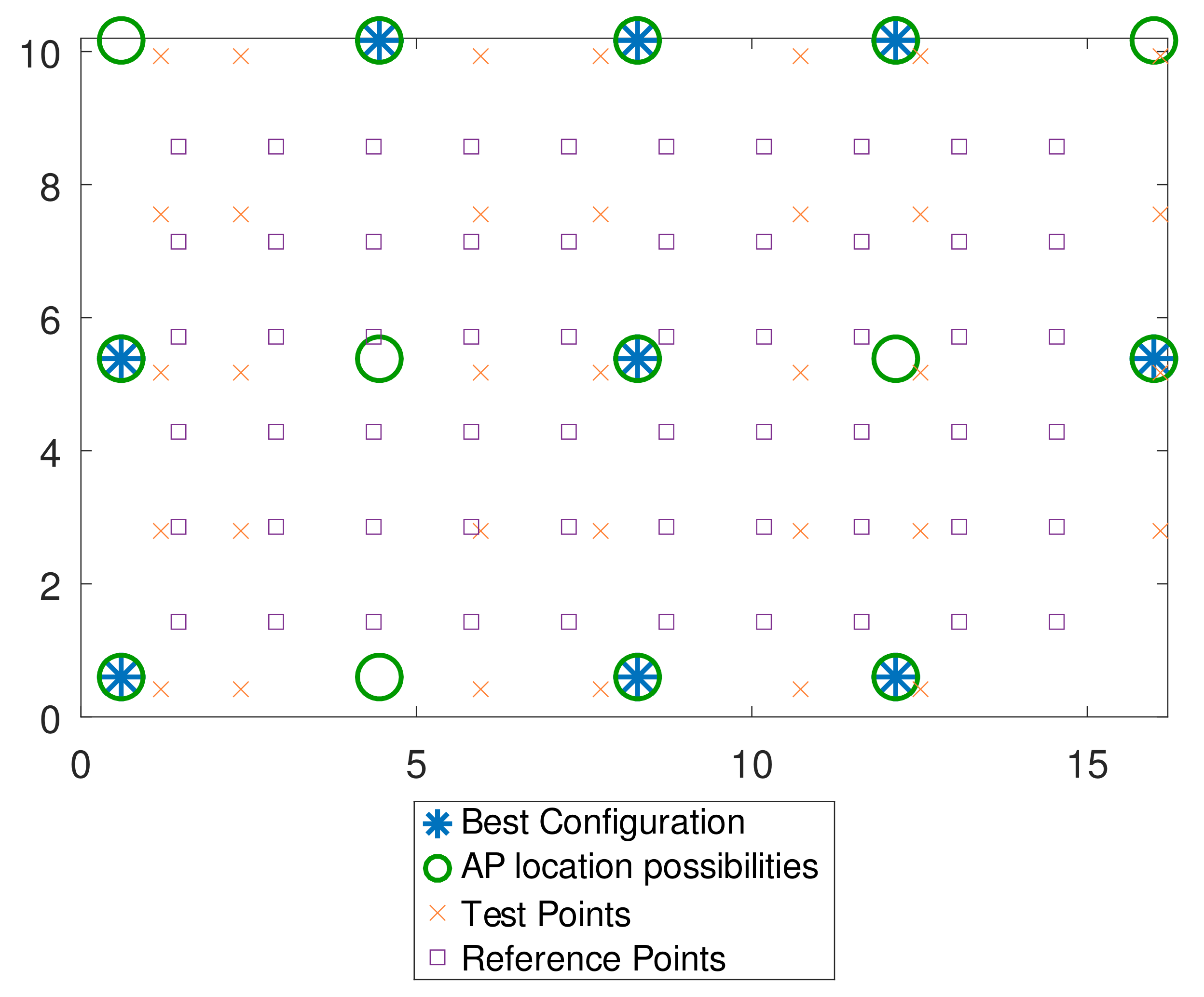
With the appropriate pre-tuning of RPs and samples, the search for an optimal arrangement of APs can be performed using the data from the fingerprints to produce a real improvement in accuracy. By considering nine APs, for instance, the best accuracy reached by simulation was the localization error of 1.42 m, concerning the combination of 60 RPs and five samples per test. This best result obtained by simulation was also reflected experimentally, in which the error reached the value of 2.40 m at 75%.
Figure 14 depicts the corresponding configuration.
Moreover, our experimental result of 2.40 m is even better than the reported in [
41] for both the k-NN and the Weighted Centroid methods with data from all 22 APs available. The errors found by Mendoza et al., in this case, were 3.34 m and 2.48 m at 75%, respectively. Thus, this is another strong indication that our proposed method can be efficiently deployed for a real IPS.
6. Conclusions
In this paper, we propose a method that is rooted in a probabilistic modeling approach to optimize the use of the most relevant factors that have an impact on the accuracy of indoor positioning systems. From the reasonable assumption that a log-distance path loss model can represent, on average, the RSS variation over an indoor area, we analyze the impact of the number of reference points, the number of samples collected per test, and the access points arrangement on the system accuracy by using a probability-based positioning technique and a simulation-based approach.
Throughout the analysis, we provide some general guidelines on how to set up the simulations by establishing reasonable intervals for the number of samples collected per test and the number of RPs. Then, a simple algorithm to go through the combinations of these factors and find the configuration with minimum localization error is proposed. Moreover, a detailed analysis regarding the time complexity of the method is discussed from a simulated case study, which highlights that the number of allocation spaces for the access points is the most limiting variable for scaling the method for larger sites.
To demonstrate and validate the proposed method, we perform tests by using a known dataset from the literature in regards to a real-world indoor scenario. The obtained results show that the combination set of design factors can be fairly reduced and can reasonably have its behavior predicted through early simulations. Besides, when restrictions of computational cost and real-time applications are relevant, the method can provide more efficient usage of the system’s inputs. Finally, the positioning accuracy obtained by our proposed method reduced the localization error up to 28% when compared to the positioning algorithms presented in the work related to the fingerprint dataset we use, which evidences our proposed solution can be an efficient alternative for the design of a real IPS.
For future work, we plan to develop an efficient algorithm to help optimize the proposed method in order to reduce its current time complexity. In this sense, the method can be scalable to larger indoor areas. In addition, we expect to improve the log-distance path loss model by considering the effects of obstructions to the model as an important variable to deal with more complex environments.


