1. Introduction
Nowadays, Cyber-Physical Systems (CPS) interact with the physical world by analyzing their environment using a variety of sensors. For this purpose, a powerful analysis tool is needed, such as Artificial Intelligence (AI), or more precisely Deep Learning (DL) algorithms. Currently, DL technologies became a hot topic in solving problems such as data analytics and object recognition [
1]. Since the late 20th century, they have evolved in a substantial way and tend to be applied in many different fields and applications related to computer science and engineering, such as CPS [
2,
3]. However, with the increased accuracy requirements and complexity of Neural Network (NN) architectures, DL technologies have been known to need a lot of computational power, mostly because of their huge number of parameters. Unlike distributed cloud computing, where a lot of processing power is available, embedded systems impel some restrictions on the use of DL technologies. Even when optimizing/compressing NN or using Graphics Processing Units (GPU) for embedded systems, there is still some possible optimization through the usage of specialized processing systems [
4,
5]. Additionally, if we want to build an application using specialized hardware processing for NN (e.g., FPGA [Field-Programmable Gate Array], ASIC [Application-Specific Integrated Circuit]), we need a complete design methodology for embedded DL in order to speed up the prototyping. In this paper, we introduce a new methodology for smart applications in CPS around DL technologies. We present and share the design of a hardware Neural Network Processor (NNP). We validate the methodology with a smart LIDAR (LIght Detection And Ranging) application case study. The new embedded DL methodology is oriented toward a hybrid CPU/FPGA-based design in order to simplify the prototyping. In this work, we share our experiences and the difficulties encountered while developing a smart LIDAR application for pedestrian detection to validate the proposed methodology. This paper is structured as follows:
Section 2 presents the related works,
Section 3 describes the proposed design methodology,
Section 4 gives details about the NNP architecture design,
Section 5 presents the experimentation results,
Section 6 is dedicated to the discussion and analysis. Finally,
Section 7 concludes this work.
2. Related Works
This work deals with two main research technologies topics around: (1) platform-based design and prototyping of deep neural network accelerator for efficient DL processing and (2) DL approaches used for 3D object classification and detection, using 3D sensors (e.g., LIDAR and a 3D camera). In this section, we give an overview and we highlight (to the best of our knowledge) the different related works that are in relation to the two main topics addressed in this work.
2.1. FPGA-Based Design and Prototyping of Deep Neural Network Accelerator
Platform-based design and prototyping have been proposed as solutions for time-to-market and design costs problems in circuits and systems design, e.g., Pinto et al. [
6], and we need to update such knowledge toward CPS using deep neural network accelerators. Platform-based design in the context of CPS was already addressed in Nuzzo et al. [
7], by proposing an approach to abstract CPS design flow. Lacey et al. [
8] presented the evolution of DL using FPGAs. They displayed different tools to design a DL accelerator on an FPGA platform, from high-level abstraction tools to deep learning framework. Sze et al. [
9] made a tutorial and survey about DNN and hardware for DNN processing. They presented efficient ways to implement co-design processing of DNN using various optimizations. Li et al. [
10] presented a survey about general-purpose processors (GPP) for neural network processing with a specific spotlight for the DianNao series accelerators. Abdelouahab et al. [
11] presented a survey about FPGA Convolutional Neural Network (CNN) accelerators. Their work was mostly about algorithm and data management optimizations. Guo et al. [
12] made a survey about FPGA neural network accelerators and summarized the different techniques used, showing that FPGA is a promising platform for neural network acceleration. Li et al. [
13] proposed a model-based design methodology involving deep NN. They proposed an integrated set of tools and libraries alongside their methodology in order to assist designers of signal processing systems. Shawahna et al. [
14] presented a survey about FPGA-based accelerators for DL networks, in particular Convolutional Neural Network (CNN), and tried to isolate a methodology for its conception. Their survey revealed a specific pattern for FPGA-based accelerated NN architecture, which is presented with techniques to optimize and automate the design. Those works were mainly focused on the design and prototyping of a deep neural network accelerator; however, there is a lack of a standard and global methodology that takes into account the design of NNP/DL in the context of an embedded application. Our work is more focused on a methodology for prototyping an embedded DL application on a hybrid CPU/FPGA platform rather than just a NN accelerator. Therefore, our interest revolves around the design and integration of deep neural network accelerators for CPS-based DL application using hybrid CPU/FPGA-based design and prototyping.
2.2. 3D Object Classification in Deep Learning
Three-dimensional object classification is a hot topic considering current sensors such as LIDAR or 3D cameras. The usage of DL application may help reach great accuracy in the classification of 3D objects. Maturana and Scherer [
15] proposed a 3D CNN using voxels as input. They proposed a way to convert a point cloud to a voxel model. Brock et al. [
16] proposed a voxel-based auto-encoder and CNN to generate and classify 3D objects. Jing Huang and Suya You [
17] proposed different 3D CNN architectures using voxels as input to classify objects. Qi et al. [
18] proposed a deep learning architecture to directly classify and segmentate point cloud instead of voxels. Zhi et al. [
19] proposed a lightweight version of 3D CNN. Three-dimensional volumetric binary voxel grid seems like a fine way to process 3D data in order to make pattern prediction for object classification. Three-dimensional object classification using DL is a hot topic because of today’s 3D sensors and the accuracy it can yield, but it is heavy on computing power.
To our knowledge, most of the proposed works are scarce of results and precise information about the reproducibility of their experiments. In our paper, we tried to share the maximum of experimentation data regarding our methodology, NNP implementation, and performance as well as source code.
3. Proposed Methodology
In this section, we propose an embedded DL-based methodology for a FPGA-based CPS platform design using a hardware NNP.
The first step of our methodology was the definition of the system with its requirements and architecture. Then, different software algorithms were designed for data processing and DL. Those algorithms were hardware accelerated using High Level Synthesis (HLS) software tools or designed from scratch with a Hardware Description Language (HDL). Finally, the hardware accelerators were synthesized and uploaded on a hardware prototype to be tested. Considering those steps, several hidden tasks were present from data processing to data management, and the configuration of a hardware prototype. The goal of our methodology was to mitigate those hidden tasks, either with simplification or automation.
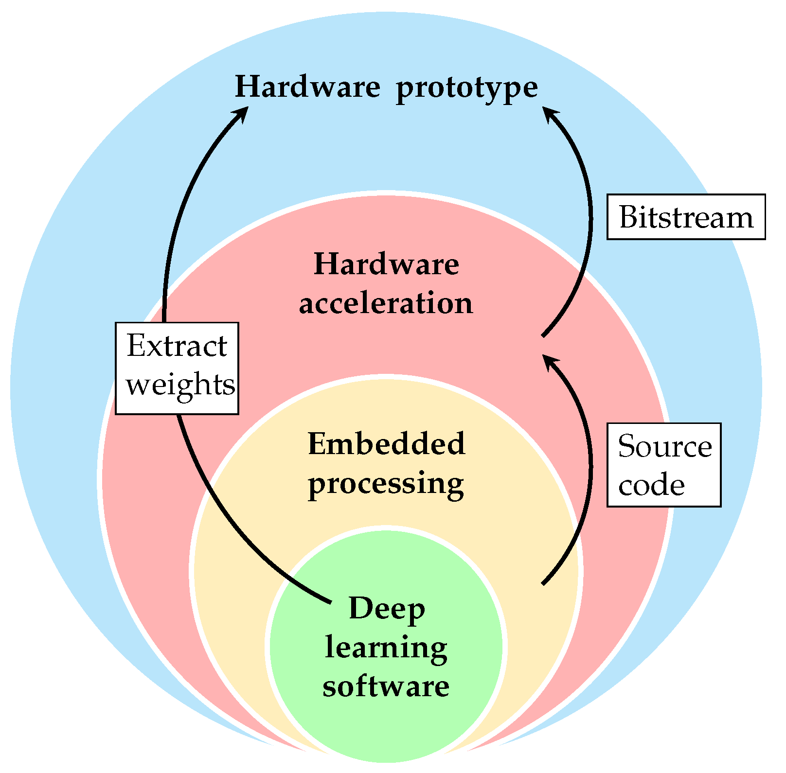
Our approach toward making a smart application for CPS was built around a FPGA-based DL methodology using an NNP. This methodology was divided in four parts (
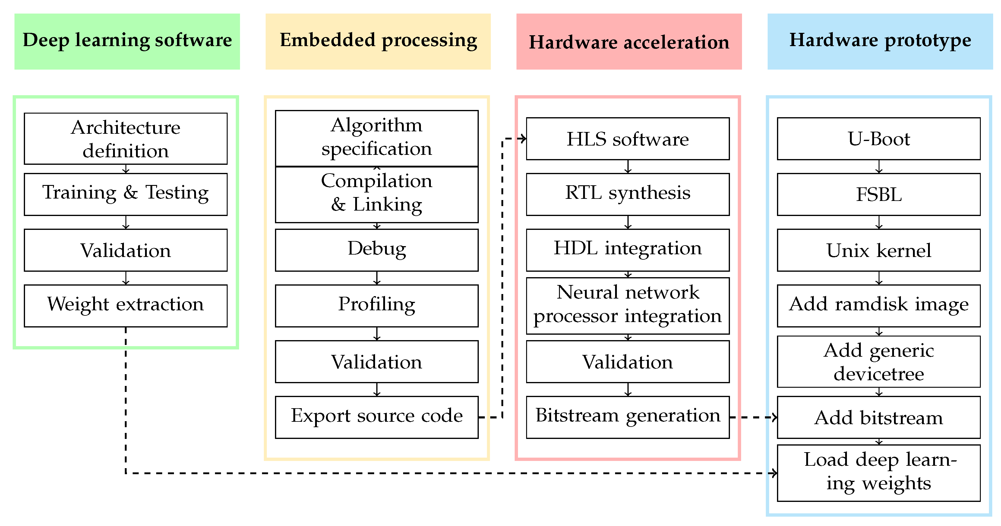
Figure 1): hardware platform, hardware acceleration, embedded processing, and DL software. The transition between each part was as follows: the DL weight matrices were extracted and transferred to the hardware platform, and the embedded processing was hardware accelerated. The development and use of the NNP as a part of the methodology was an important step in order to handle the DL processing. The description of the methodology was made with a top-to-bottom approach by disassembling the different tasks to make a prototype and by explaining our design process to share our experiences. A design flow detailing the approach of our proposed methodology is presented in
Figure 2. It shows the different steps of the four parts of the methodology and indicates how the parts are connected to each other.
Our proposed methodology for embedded DL differs from standard ones because of its constraints. The differences are mostly about integration of the NNP and its associated configuration software.
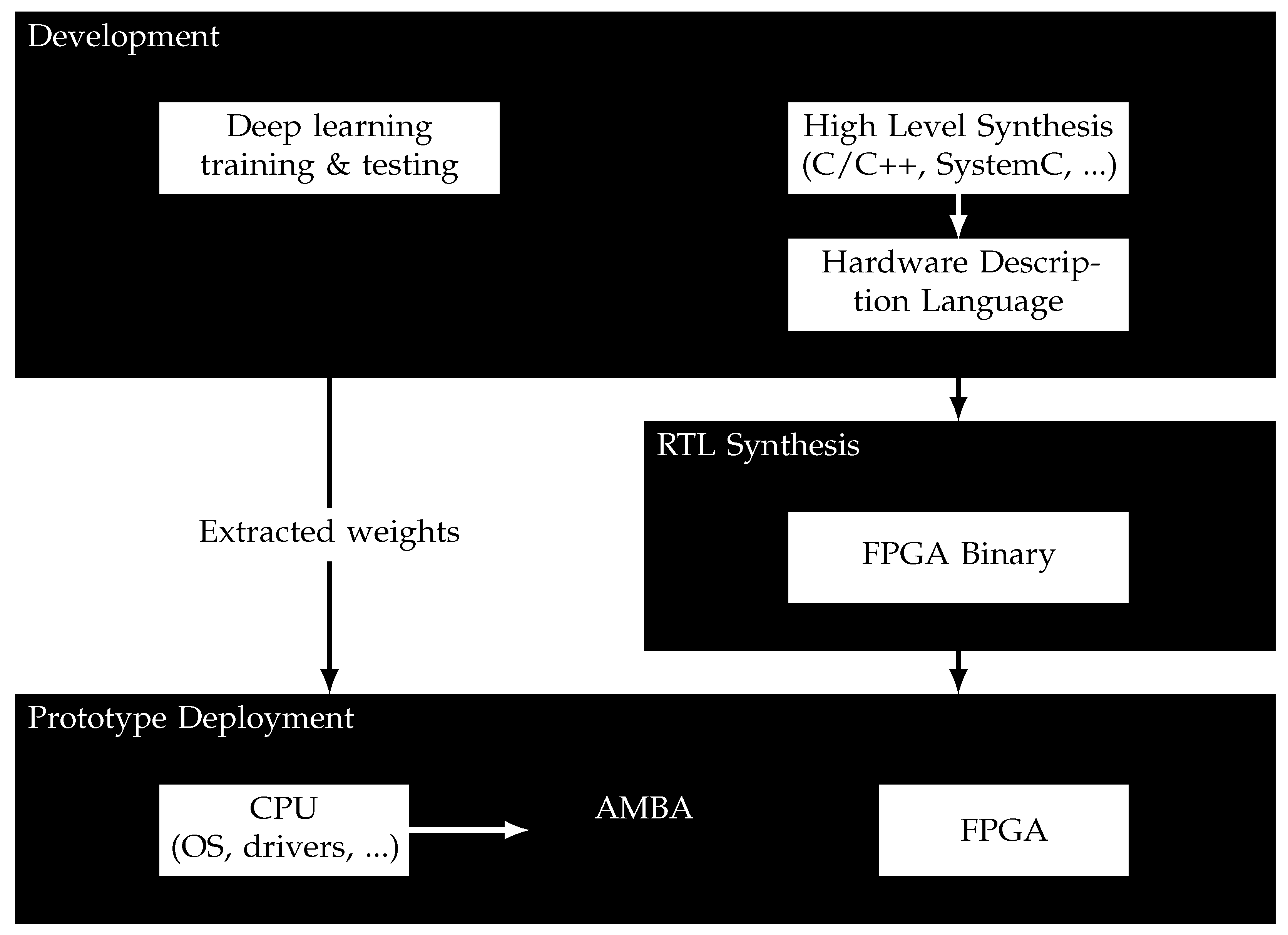
Figure 3 illustrates the implementation of our methodology. Our DL processing was based on a hardware NNP that we created. In order to create it, we first designed it as a software using event-driven simulation interface (SystemC) and then migrated it to a hardware accelerator using HLS tools. This NNP could be considered a fully functional Intellectual Property (IP) to be integrated alongside the other IPs from the hardware-accelerated embedded processing. This processor used the extracted weight matrices, which came from the offline DL training and testing.
3.1. Hardware Prototype
One contribution of this work is to develop a real prototype by acquiring physical data from the real world and by processing it in order to obtain an accurate analysis. This analysis was conducted by transforming physical data into specific features that were used with a DL approach to be classified. The hardware prototype needed to host an embedded processing application to transform physical data as features for an NN so that data could be classified by our DL application (NNP). Hence, the hardware prototype hosted an FPGA bitstream containing hardware-accelerated embedded processing to calculate features from data as well as the NNP IP classifying those data. We also needed to set up the hardware prototype with an OS and a devicetree in order to execute the FPGA control software. The hardware prototype setup was automated with an automation tool that we developed for this case [
20]. This tool deployed a bootloader (U-Boot) and a First Stage Bootloader (FSBL) to help obtain the first stages of the platform. The tool also deployed a Unix kernel with its initial ramdisk, preconfigured system files, and a generic devicetree to gain access to all components on the hardware prototype. Once set up, the hardware prototype needed software to control the FPGA processing as well as to transmit data between the different processing elements, since most data are available inside the platform DRAM to act as an interface between the different processing components, such as CPU and FPGA.
3.2. Hardware Acceleration
The embedded processing was built as an FPGA hardware IP. The hardware accelerator development was simplified using HLS software tools or HDL, but data management was still a sensitive part of the development because of the FPGA constraints. In this methodology, we considered that data is received and transmitted as a FIFO (First In, First Out) queue in order to simplify data management, even if it may mean extra calculation for processing tasks. This led to the embedded processing application receiving data from sensors and directly transmitting the processed information to the NNP. It also meant that the NNP received its data (input vector and weight matrices) as a FIFO queue and needed to compute the classification as data transmission progress. The embedded processing algorithms needed to be tweaked in order to compute FIFO transmitted data and used the smallest amount of internal cache (BRAM) possible, since FPGA does not have infinite internal memory. We mainly considered the usage of a HLS software to synthesize embedded processing software from High Level Language (HLL) to Register-Transfer Level (RTL), thus smoothing the software to hardware transfer.
3.3. Embedded Processing
The data perceived by the CPS should be processed so the NNP can use it correctly. It is necessary for two main reasons: (1) the data needs to be transformed for the NN to handle it and (2) to decrease the size of the neural network by computing some features beforehand. The main constraint is about data management. With data as a FIFO queue, most algorithms need to be redesigned in order to use as little memory cache as possible.
3.4. Deep Learning Software
A common method to make a DL application is by using specific tools to train and test NN architectures with a dataset. In this work, we considered the NN architecture as already defined. We also considered offline training as already conducted. The weights were then extracted to be used directly by the NNP embedded in the hardware platform. In this methodology, we considered weights extracted as a binary file containing the weight matrices between all layers.
4. Neural Network Processor Implementation
The NNP was designed to simplify the integration of DL in embedded CPS applications. To keep this processor simple, some constraints were defined: process the simplest NN architecture (fully connected NN without bias) with as few activation functions as possible, process any number of layers independently of their depth and width, and be re-configurable at runtime. A no-bias architecture was chosen here because bias calculation needs more computational power and time.
Computing a fully connected NN, also called Dense Neural Network (DNN), is mainly about matrix calculation. The main problem that arises from the implementation is not related to computation but data management. Weight matrices need to be loaded from external memory to be transmitted afterwards to the FPGA in order to allow for different configurations and because of the limited FPGA memory cache (BRAM) compared to the size of nowaday weight matrices that can reach dozens of megabits when using 32-bit floating-points. However, to optimize data transmission, each hidden layers’ output needs to be kept in FPGA cache. Moreover, weights need to be sorted correctly depending on the scheduling for neuron processing units. In this implementation, inputs and weights are floating-point numbers and no compression is currently done.
In order to correctly control and configure this NNP, a configuration software is made which has for its main tasks loading binary files containing weight matrices to the DRAM, preparing the instructions for the NNP depending on each weight matrix dimension, and initializing DMA transmissions.
4.1. Neural Network Processor Architecture
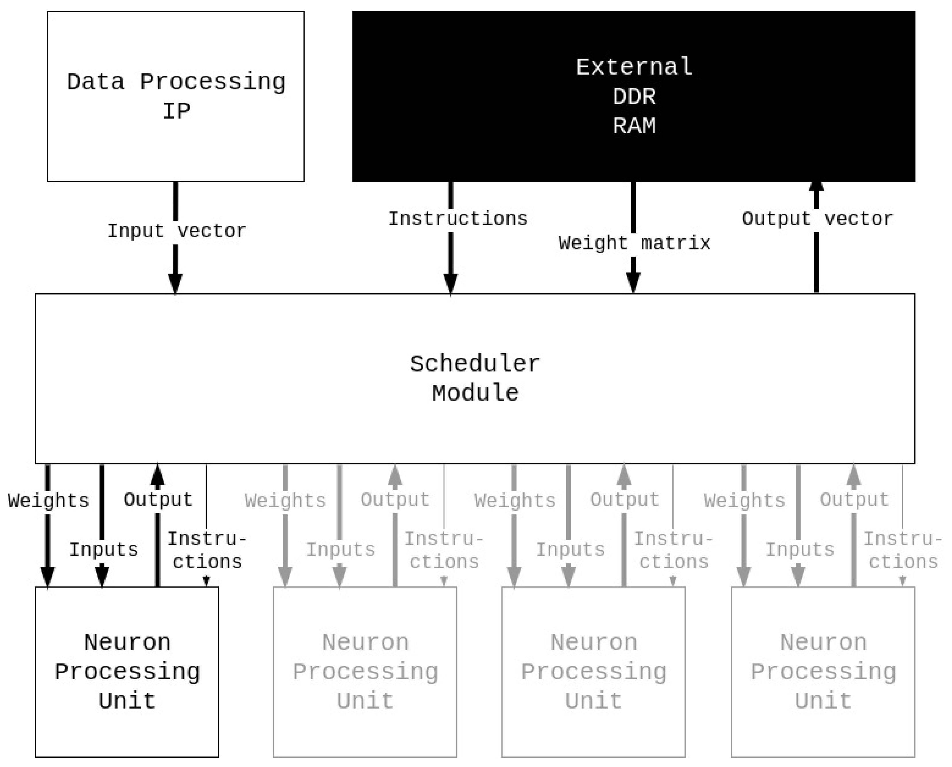
First, we detail the hardware architecture of the NNP and how it calculates layers and neurons.
Figure 4 represents the different parts of the processor and the communication interfaces in-between. There are four communication channels with the NNP for different data: the input vector, which comes directly from the embedded processing; the instructions and weight matrix, which are loaded from the external DRAM; and the output vector, which is loaded into the external DRAM.
4.1.1. Scheduler Module
The scheduler module loads all of the instructions from the DRAM to know how many weights and inputs should be loaded and the activation function to be used for each layer. Each instruction represents information about one layer and is coded by a 64-bit word containing three pieces of information: the number of neurons in the previous layer (30 bits), the number of neurons in this layer (30 bits), and the activation function of this layer (4 bits).
Once all instructions are loaded, the input vector is read from the data processing IP (Intellectual Property) into a local cache and the processing is started. For each layer, each neuron is represented by a neuron processing unit, also called a core, and thus, each neuron is computed individually. The scheduler starts a core by sending specific instructions to it, which are not the same as the ones that the scheduler module is receiving. Then, each input and weight connected to the specific computed neuron is sent. Once the core has finished the calculation, the output is returned to the scheduler, which stores it in the local cache (BRAM) to be used for the next layer. Once all neurons of the layer are computed, the output vector is used as the input vector of the next layer and the process starts again. Once the last layer is reached, the output vector of the NNP is written to the external DRAM. Algorithm 1 describes in a shorter way the scheduler module process.
| Algorithm 1: Scheduler module algorithm. |
![Jsan 10 00018 i001]() |
Because of the size of the number of neurons in the scheduler module instructions (30 bits), a layer should be able to have over 1 billion nodes. However, there is a hard limit inside the scheduler module cache (BRAM) for resource utilization purposes, which means that a layer cannot be larger than 65,536 nodes. The number of instructions that can be loaded in the scheduler is set to 512, which makes the instructions buffer size 4096 bytes. Thus, the scheduler module uses at least 528,384 bytes of FPGA memory cache. The resources used for the hardware scheduler component is showed in
Table 1.
4.1.2. Neuron Processing Unit
Each neuron processing unit calculates one neuron at a time. It takes instructions from the scheduler module, each instruction is a 34 bit word containing two pieces of information: the number of inputs and weights (30 bits) and the activation function to be used (4 bits). When an instruction is received, the processing engine module starts listening to weights and inputs. Each time a pair of inputs and weights are received, they are multiplied and summed to previous results. Once all inputs and weights for one neuron are received, the activation function is calculated and sent to the output. Algorithm 2 describes in a shorter way to process the engine module process.
| Algorithm 2: Neuron processing unit algorithm. |
![Jsan 10 00018 i002]() |
As said before, the activation functions are limited to four activation functions:
relu,
linear,
sigmoid, and
softmax.
Relu,
linear, and
sigmoid activation functions are computed directly inside the neuron processing unit. However, in the case of the
softmax activation function, the exponential part is performed in the neuron processing unit and the division by the sum of the output vector is performed inside the scheduler module because only the scheduler has access to the whole output vector. All the SystemC source code we wrote for the NNP is available online [
21]. A testbench is available to load datasets and neural network models. The synthesis for each of those components is done using Vivado HLS [
22]. The resources used for the hardware neuron processing component is shown in
Table 2.
4.2. Configuration Software
Once the hardware was designed, a software stack was needed to load data into the DRAM to control the NNP. This software’s purposes are twofold: to read a configuration file that regroups all weight matrices inside a binary file in order to determine from it the network topology and to generate instructions as well as to sort all weights in matrices for scheduling purposes. The weight matrices were then written in the external DRAM waiting to be read by the NNP, which was started and waited for the input vector from the data processing IP. Every time the NNP finished a calculation, the output vector was read from the external DRAM. Control of the NNP was performed through DMA registers since it is always waiting for instructions. Algorithm 3 describes how the configuration software behaves.
| Algorithm 3: NNP configuration software algorithm. |
![Jsan 10 00018 i003]() |
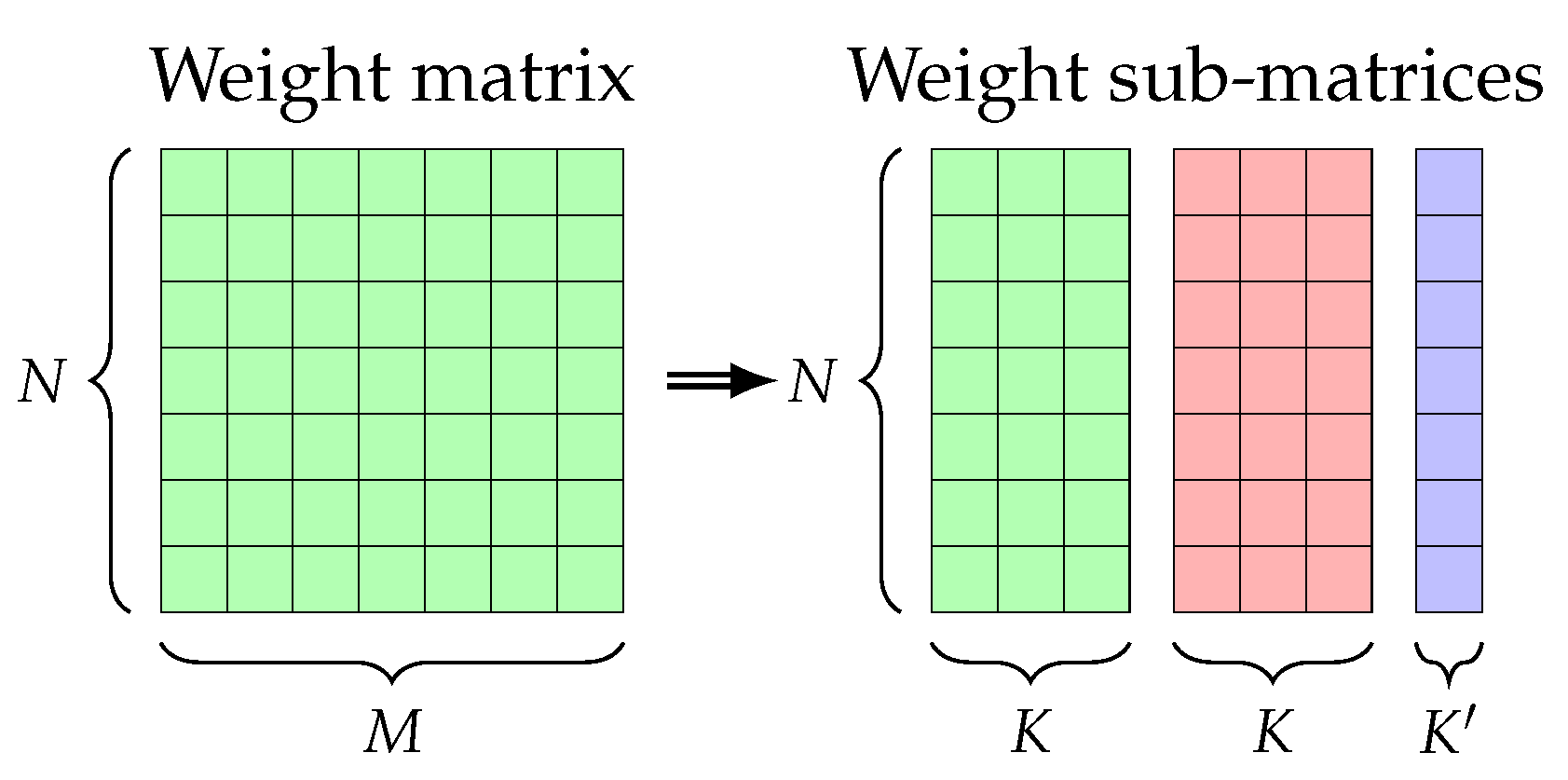
Regarding weight sorting, since data were a FIFO queue and to reduce data memory cache usage inside the FPGA, the weights were transmitted in the same order as the transmissions to their associated neuron processing unit. The scheduling algorithm loaded all pairs of inputs and weights to each core until all neurons were processed. This means that weights must be sorted depending on layer size and the number of available cores. The basic process is about dividing the weight matrix into sub-matrices with a size depending of the number of available cores (
Figure 5). Each sub-matrix represents the weights for one set of
K neuron processing units. Those weights needed to be sorted by processing unit, and this was done with a transposition. Then, each transposed matrix was vectorized for memory writing purposes. All vectors were then merged into one vector and written into the DRAM.
5. Experimentation and Results
In this section, two experiments are presented: the test and validation of our NNP and the smart LIDAR for pedestrian detection case study. The NNP test and validation present the time performance and accuracy of our processor. The smart LIDAR case study is made to test our proposed methodology alongside the NNP. We propose to share our experiments on a smart LIDAR for object classification application and the results of this experiment. We describe in detail the workflow and each component of the application as well as performance and resource utilization. It is noted that there is no real LIDAR involved in this work; we instead used the 3D Point Cloud People Dataset acquired from a Velodyne HDL 64E S2 sensor [
23,
24]. This dataset recorded real-world data in downtown Zurich (Switzerland) and recorded mostly pedestrians. The main goal of this validation is to determine if we can detect them by designing an application using our proposed methodology.
5.1. NNP: Test and Validation
Tests were done on a Zedboard development kit [
25] using the Xilinx Zynq-7000 SoC (XC7Z020) [
26]. Each test corresponds to the usage of a specific known dataset with a specific NN architecture for each dataset. NN model training and testing were done with Tensorflow [
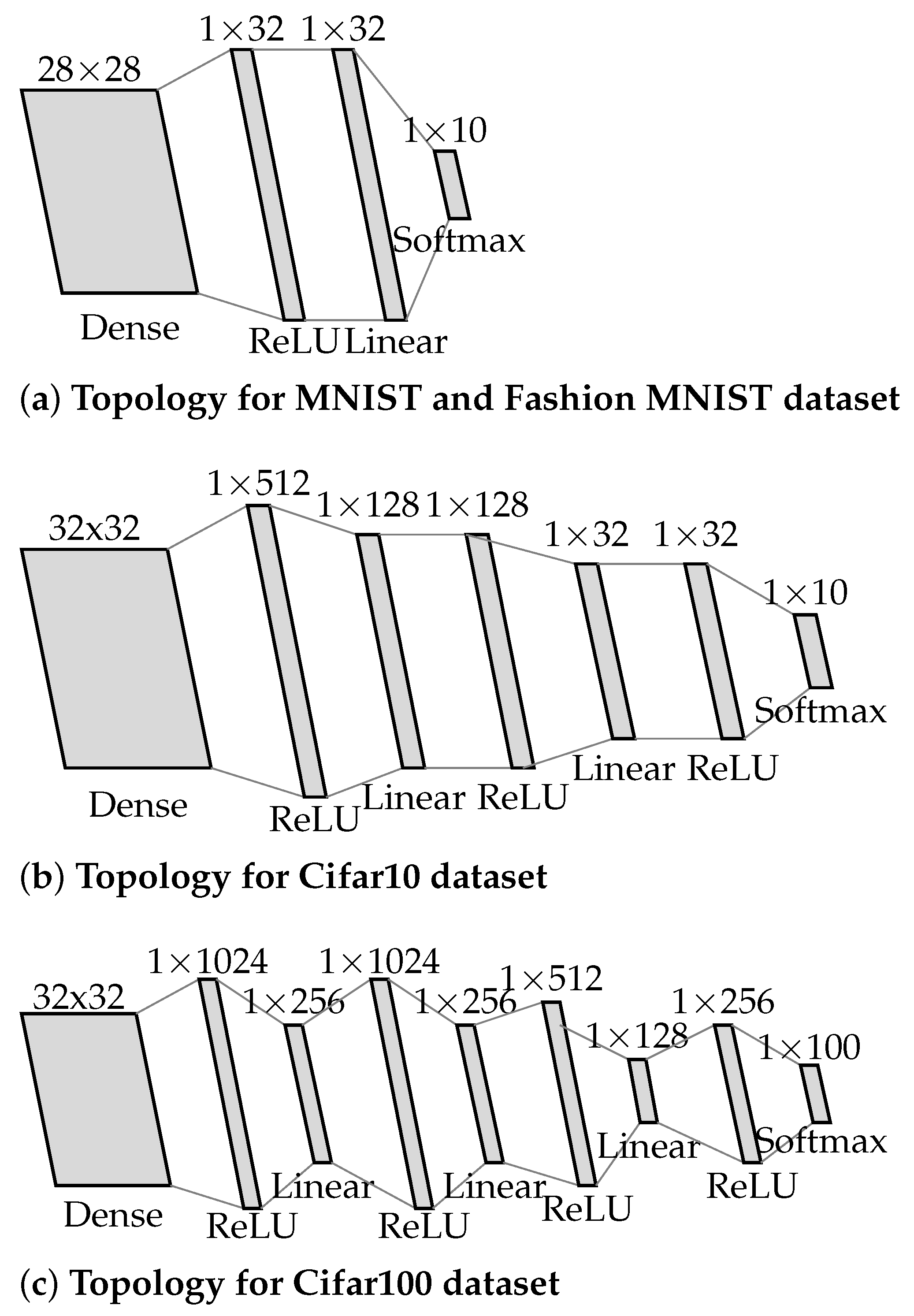
27]. NN topologies are shown in
Figure 6.
Table 3 compares the accuracy results for each dataset achieved by our NNP depending on its number of cores and the Tensorflow software executed on a CPU. These results mean that our NNP correctly computes floating-point numbers without error. It is noted that the maximum number of cores possible on this FPGA platform is 4 because of the DSP (Digital Signal Processor) limitation (220 DSP available on our FPGA platform with each core using 48 DSP; see
Table 2).
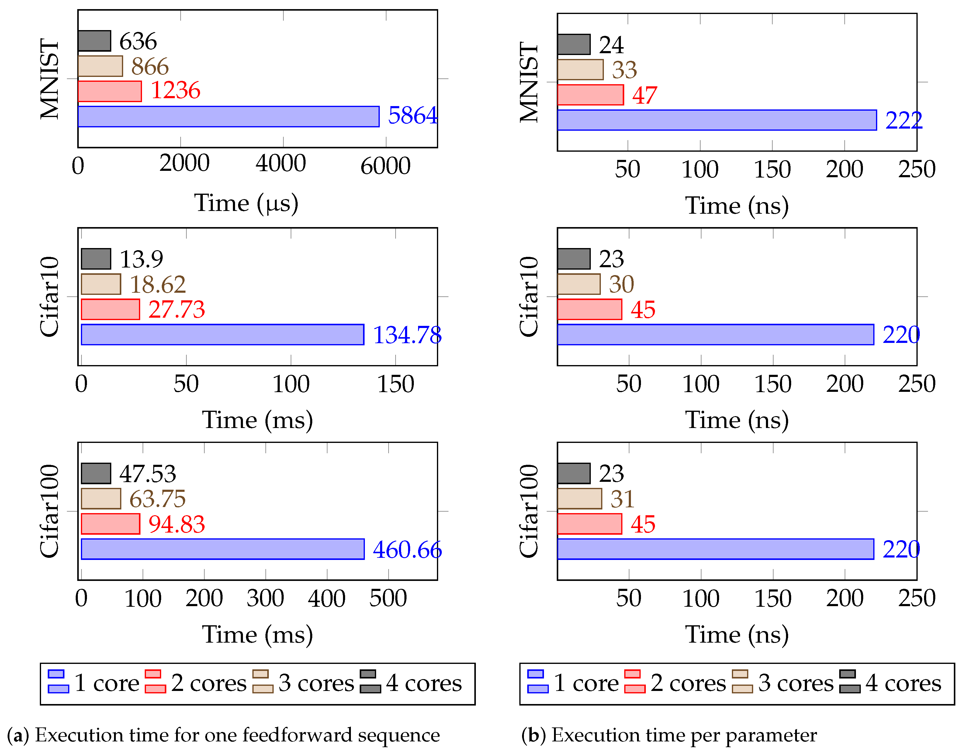
In this work, the execution time is our main concern, and it is obviously related to the number of parameters in the NN and the number of cores in the processor.
Figure 7a shows the execution time of three datasets depending on the number of cores. The execution time seems to be close to linear, with a same architecture and a different number of cores, except for when there is only one core, which shows a bottleneck. Moreover, the execution time per parameter seems to be the same between the different datasets, as shown in
Figure 7b. With Vivado HLS transforming the SystemC models to HDL, our hardware threads run in parallel (the scheduler and neuron processing units are independent finite state machines using the same clock). The clock for the hardware threads runs at 100 MHz, which is 150 MHz lower than the maximal frequency on our hardware. However, increasing more than this frequency means that time constraints are not met. The use of parallel hardware threads improved the processing time of our system. However, we want to point out the data transfer bottleneck in the AXI system bus, which affects the whole processing time of the system. This bottleneck is mainly due to the number of parameters transmitted. Since we use 32-bit floating points, the parameters matrices of the NN are in the MB scale and our AXI channels run at a theoretical maximum of 300 MB/s. We would obtain better results if we used compression such as 16-bit fixed point integer or binary weights. Another option to improve the time consumption would be to run the scheduler which controls the neural processing units with a faster clock than the neuron processing units so that data are read faster from DMA and distributed faster to the processing units, but we did not confirm that this will bypass the data transfer bottleneck. In the context of the defined topologies, MNIST [
28] has 26,432 parameters, Cifar 10 [
29] has 611,648 parameters (because, since the input is grayscaled, the image size is 32 × 32 × 1), and Cifar 100 [
29] has 2,089,984 parameters. In
Figure 7b, the analysis shows that the execution time of the feed forward sequence of a specific NN model may be predicted. This means that we can determine the needed NNP cores for a given application with real-time constraints.
5.2. Smart LIDAR for Pedestrian Detection Case Study
The first step of this experiments was to define the workflow of the application.
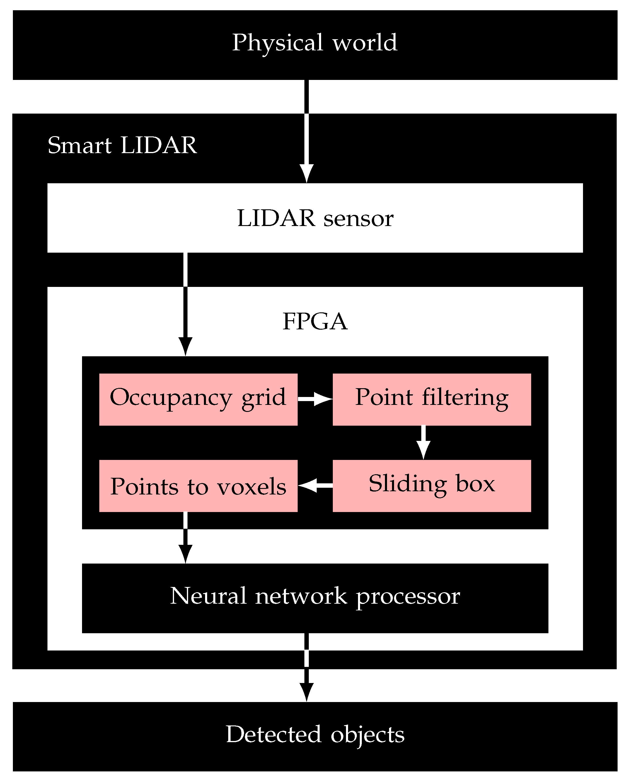
Figure 8 represents all the steps of the application. It first starts with the physical world data that were acquired through the LIDAR sensor. The sensor transmits its raw data to the embedded processing hardware IP in order to process and transform the information so it can be used by the NNP IP and then analyzed the data and classified the objects.
5.2.1. Deep Learning Software
The first step when working on this prototype was to define how to classify objects from 3D data, such as the point cloud received from the LIDAR. One way to classify objects is to convert point cloud to voxels and then to use deep learning to determine the category [
15]. The dataset used in our case study was the Sydney Urban Objects Dataset (SUOD) [
30,
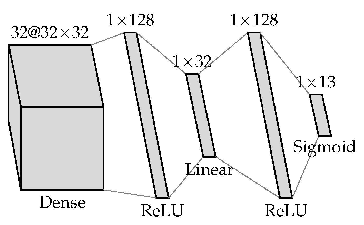
31], but we converted point clouds into a 32 × 32 × 32 voxel grid using a volumetric binary occupancy grid approach. The training was performed with the architecture represented in
Figure 9 using Tensorflow software [
27]. The hardware used for the training was 16 GB of RAM with an Intel Core i7-8550U CPU with 4 cores, 8 threads, a base frequency of 1.8GHz up to a turbo frequency of 4 GHz, as well as a 8 MB cache. Once the architecture was defined and the training/testing was performed, the weights were extracted in a NumPy binary format [
32].
5.2.2. Embedded Processing
Three-dimensional point cloud data were the input of the smart LIDAR. Each object in the point cloud needed to be extracted and transformed to voxels as an input for the NNP. To achieve this, four tasks were needed, as shown in
Figure 8. The first step was to make an occupancy grid to detect objects inside the point cloud. The second step was to remove all points that were not considered objects. The third step was to isolate objects with a “sliding box”. The results for those three steps were presented in a previous paper [
33]. The fourth step was to convert extracted objects into a volumetric binary occupancy grid. Once the object was transformed into a 32 × 32 × 32 voxel grid, it was sent to the NNP. The embedded processing was written in SystemC and synthesized to RTL with an HLS software (Xilinx Vivado HLS [
22]). The algorithm for the “points to voxels” module is presented in Algorithm 4. The module received all the points from a box two times: the first time to calculate the bounding box and the second time to calculate the volumetric binary occupancy grid. The input and ouput of the “points to voxels” module are shown in
Figure 10. The pedestrians were extracted in boxes of 2 × 2 × 2 meters and then converted to a 32 × 32 × 32 voxel grid. The FPGA synthesized results are shown in
Table 4. After the hardware IPs implewere mented, we tested all extracted pedestrian boxes to find the mean execution time per point (
Table 5).
| Algorithm 4: Point cloud to voxel grid (embedded processing). |
![Jsan 10 00018 i004]() |
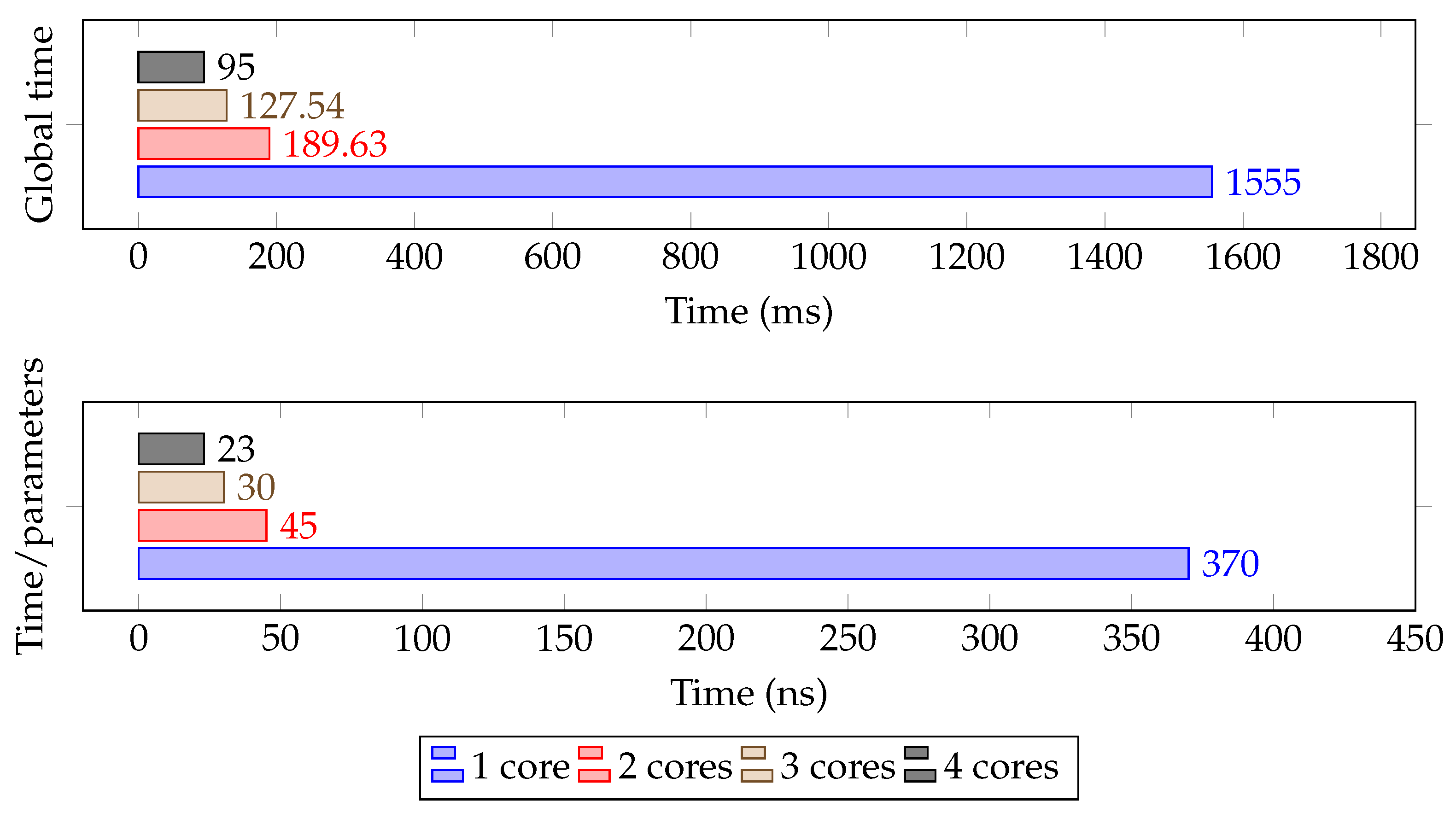
5.2.3. Neural Network Processor
The embedded processing was synthesized with the NNP. The bitstream was then ported on top of the platform. The hardware platform used was a ZedBoard Zynq-7000. The SD card generation was automated using our script [
20]. This script deploys a UNIX operating system (OS) and all other required resources to boot this OS. The weight matrices were also integrated within the SD card along with the configuration software. In order to evaluate the system, two tests were performed. The first test was related to the SUOD. The accuracy was evaluated with all classes contained in the dataset. The second test was related to the 3D Point Cloud People Dataset. We extracted all pedestrian boxes from the Polyterrasse set to test if they were correctly classified, which means 599 fully visible pedestrians. Thus, the accuracy is related to the number of boxes that were correctly classified as pedestrians. With 4,204,160 parameters, the processing time of this network topology is shown in
Figure 11. The results are shown in
Table 6. The results of the SUOD accuracy for multiple object detection is really low compared to state-of-the-art neural networks. This is mainly due to two things: the use of dense NN instead of CNN, and the limited number of parameters in the NN compared to the number of classified objects. However, when trying to apply the same topology to only detecting pedestrians, the results are far better, which means that the use of dense NN and the number of parameters are enough to classify one type of object.
6. Discussion
The investigation of embedded DL within the design and prototyping of CPS using Multi-CPU/FPGA platforms shows that our proposed methodology simplifies the prototyping of DL-based CPS systems (e.g., autonomous vehicles). The critical step of the proposed methodology is the design and integration of the NNP. It is considered an accelerator for DL computation and mainly for the inference step. It also simplifies migration from the software deep learning to the hardware platform. This work is also considered a first step in simplifying the prototyping process of embedded DL for CPS. The scope of this methodology can cover DL applications dedicated to embedded classification in constrained environments. Our proposed methodology is oriented toward DNN topologies. In such embedded contexts, migration of the DL processing from CPU to hardware accelerators would increase the performance of the whole system, reaching specific real-time constraints and making the inference step easier for optimized embedded AI. Even if the NNP integration step is not automated yet, it is portable for several applications and platforms. In addition, the current NNP can be improved at several levels: (1) data management needs to be refactored and optimized in order to speed up computation, (2) a flexible architecture is needed to integrate more activation functions and topology types. Moreover, we think that the use of the Vivado HLS software tool to implement the NNP might slow down the final design compared to a from scratch HDL model. Currently, our NNP is adapted for lightweight neural networks since the execution time might be enough to reach real-time constraints in some applications while using low power. Although the limited topology and activation functions choice might be a constraint for some applications, NNP design reuse, in the context of platform based design for CPS systems, is a motivation for us to investigate the possibility of automated generation of this NNP with the needed number of cores and then the automation of the whole methodology, since several steps are already automated using our automation software. In fact, attempting to automate such generations for every case is not a realistic goal. However, we are convinced that automation of the NNP integration in the whole design methodology would present a huge improvement in terms of design time, exploration, prototyping, and CPS systems portability.
7. Conclusions
In this paper, a new methodology for Cyber-Physical Systems (CPS) design and prototyping is presented. It is defined around an embedded Deep Learning (DL) approach. In order to compute this embedded DL algorithm, we propose a new hardware Neural Network Processor (NNP) architecture. We also share our experience of the design/implementation and the porting of the DL-based NNP on a real hardware Multi-CPU/FPGA platform (Zynq). Our DL-NNP model used real data coming from a LIDAR sensor. Hardware threads were used to transform data from a 3D Point Cloud (LIDAR) to a voxel grid, which is considered the input of our NNP. Results related to the NNP performances are presented, and the whole methodology is validated with a smart LIDAR for pedestrian detection case study. The prediction of the NNP execution time is dependent on the number of parameters (weight matrices) in the Neural Network (NN) and the number of NNP cores. We still have some work to do to optimize the proposed NNP. In future work, we aim to automate generation and integration of the NNP. We want to simplify the design reuse of our NNP with automation. The work presented in this paper is a first step to understanding the design and implementation of Artificial Intelligence (AI) in the context of embedded systems related to CPS. The proposed methodology, which is oriented toward an embedded hardware DL based on FPGA, shows real progress in understanding the harsh relation between the embedded world, AI, and CPS. Through this work, we defined the different steps of this relation. We think that the automation of those steps will be extremely helpful for embedded AI designers to simplify the prototyping steps and to move toward more significant design space exploration.
Author Contributions
Conceptualization, Q.C., B.S. and A.R.-C.; methodology, Q.C. and B.S.; software, Q.C.; validation, Q.C. and B.S.; formal analysis, Q.C.; investigation, Q.C. and B.S.; resources, B.S. and A.R.-C.; data curation, Q.C.; writing—original draft preparation, Q.C. and B.S.; writing—review and editing, Q.C., B.S. and A.R.-C.; visualization, Q.C.; supervision, B.S. and A.R.-C.; project administration, B.S. and A.R.-C.; funding acquisition, B.S. and A.R.-C. All authors have read and agreed to the published version of the manuscript.
Funding
This research received no external funding.
Informed Consent Statement
Not applicable.
Data Availability Statement
Data available in a publicly accessible repository that does not issue DOIs. All link and repositories are in the references of this article.
Acknowledgments
We want to thank the INSEEC U Research Center for funding this research work.
Conflicts of Interest
The authors declare no conflict of interest.
References
- LeCun, Y.; Bengio, Y.; Hinton, G. Deep learning. Nature 2015, 521, 436–444. [Google Scholar] [CrossRef] [PubMed]
- Wickramasinghe, C.S.; Marino, D.L.; Amarasinghe, K.; Manic, M. Generalization of Deep Learning for Cyber-Physical System Security: A Survey. In Proceedings of the IECON 2018—44th Annual Conference of the IEEE Industrial Electronics Society, Washington, DC, USA, 21–23 October 2018; IEEE: Washington, DC, USA, 2018; pp. 745–751. [Google Scholar] [CrossRef]
- Arif, A.; Barrigon, F.A.; Gregoretti, F.; Iqbal, J.; Lavagno, L.; Lazarescu, M.T.; Ma, L.; Palomino, M.; Segura, J.L.L. Performance and energy-efficient implementation of a smart city application on FPGAs. J. Real-Time Image Process. 2018. [Google Scholar] [CrossRef] [Green Version]
- Wang, C.; Yu, Q.; Gong, L.; Li, X.; Xie, Y.; Zhou, X. DLAU: A Scalable Deep Learning Accelerator Unit on FPGA. arXiv 2016, arXiv:1605.06894. [Google Scholar] [CrossRef]
- Birk, M.; Zapf, M.; Balzer, M.; Ruiter, N.; Becker, J. A comprehensive comparison of GPU- and FPGA-based acceleration of reflection image reconstruction for 3D ultrasound computer tomography. J. Real-Time Image Process. 2014, 9, 159–170. [Google Scholar] [CrossRef]
- Pinto, A.; Bonivento, A.; Sangiovanni-Vincentelli, A.L.; Passerone, R.; Sgroi, M. System level design paradigms: Platform-based design and communication synthesis. ACM Trans. Des. Autom. Electron. Syst. 2006, 11, 537–563. [Google Scholar] [CrossRef]
- Nuzzo, P.; Sangiovanni-Vincentelli, A.L.; Bresolin, D.; Geretti, L.; Villa, T. A Platform-Based Design Methodology With Contracts and Related Tools for the Design of Cyber-Physical Systems. Proc. IEEE 2015, 103, 2104–2132. [Google Scholar] [CrossRef] [Green Version]
- Lacey, G.; Taylor, G.W.; Areibi, S. Deep Learning on FPGAs: Past, Present, and Future. arXiv 2016, arXiv:1602.04283. [Google Scholar]
- Sze, V.; Chen, Y.H.; Yang, T.J.; Emer, J. Efficient Processing of Deep Neural Networks: A Tutorial and Survey. arXiv 2017, arXiv:1703.09039. [Google Scholar] [CrossRef] [Green Version]
- Li, Z.; Wang, Y.; Zhi, T.; Chen, T. A survey of neural network accelerators. Front. Comput. Sci. 2017, 11, 746–761. [Google Scholar] [CrossRef]
- Abdelouahab, K.; Pelcat, M.; Serot, J.; Berry, F. Accelerating CNN inference on FPGAs: A Survey. arXiv 2018, arXiv:1806.01683. [Google Scholar]
- Guo, K.; Zeng, S.; Yu, J.; Wang, Y.; Yang, H. [DL] A Survey of FPGA-based Neural Network Inference Accelerators. ACM Trans. Reconfig. Technol. Syst. 2019, 12, 1–26. [Google Scholar] [CrossRef]
- Li, L.; Sau, C.; Fanni, T.; Li, J.; Viitanen, T.; Christophe, F.; Palumbo, F.; Raffo, L.; Huttunen, H.; Takala, J.; et al. An integrated hardware/software design methodology for signal processing systems. J. Syst. Archit. 2019, 93, 1–19. [Google Scholar] [CrossRef]
- Shawahna, A.; Sait, S.M.; El-Maleh, A. FPGA-Based Accelerators of Deep Learning Networks for Learning and Classification: A Review. IEEE Access 2019, 7, 7823–7859. [Google Scholar] [CrossRef]
- Maturana, D.; Scherer, S. VoxNet: A 3D Convolutional Neural Network for real-time object recognition. In Proceedings of the 2015 IEEE/RSJ International Conference on Intelligent Robots and Systems (IROS), Hamburg, Germany, 28 September–2 October 2015; IEEE: Hamburg, Germany, 2015; pp. 922–928. [Google Scholar] [CrossRef]
- Brock, A.; Lim, T.; Ritchie, J.M.; Weston, N. Generative and Discriminative Voxel Modeling with Convolutional Neural Networks. arXiv 2016, arXiv:1608.04236. [Google Scholar]
- Huang, J.; You, S. Point cloud labeling using 3D Convolutional Neural Network. In Proceedings of the 2016 23rd International Conference on Pattern Recognition (ICPR), Cancun, Mexico, 4–8 December 2016; IEEE: Cancun, Mexico, 2016; pp. 2670–2675. [Google Scholar] [CrossRef]
- Charles, R.Q.; Su, H.; Kaichun, M.; Guibas, L.J. PointNet: Deep Learning on Point Sets for 3D Classification and Segmentation. In Proceedings of the 2017 IEEE Conference on Computer Vision and Pattern Recognition (CVPR), Honolulu, HI, USA, 21–26 July 2017; IEEE: Honolulu, HI, USA, 2017; pp. 77–85. [Google Scholar] [CrossRef] [Green Version]
- Zhi, S.; Liu, Y.; Li, X.; Guo, Y. LightNet: A Lightweight 3D Convolutional Neural Network for Real-Time 3D Object Recognition. In Proceedings of the Eurographics Workshop on 3D Object Retrieval, Lyon, France, 23–24 April 2017; p. 8. [Google Scholar] [CrossRef]
- Cabanes, Q. Automation Script of Bootable SDcard for Zynq Board. 2018. Available online: https://github.com/Tigralt/zynq-boot (accessed on 22 February 2021).
- Cabanes, Q. Hardware Neural Network Processor. 2020. Available online: https://github.com/Tigralt/hardware-neural-network-processor (accessed on 22 February 2021).
- Xilinx. Vivado Design Suite HLx Editions, 2018.3. Available online: https://www.xilinx.com/support/download/index.html/content/xilinx/en/downloadNav/vivado-design-tools/archive.html (accessed on 22 February 2021).
- Spinello, L.; Arras, K.O.; Triebel, R.; Siegwart, R. A Layered Approach to People Detection in 3D Range Data. In Proceedings of the AAAI Conference on Artificial Intelligence (AAAI), Atlanta, GR, USA, 11–15 July 2010; p. 6. [Google Scholar]
- Spinello, L.; Luber, M.; Arras, K.O. Tracking people in 3D using a bottom-up top-down detector. In Proceedings of the 2011 IEEE International Conference on Robotics and Automation, Shanghai, China, 9–13 May 2011; IEEE: Shanghai, China, 2011; pp. 1304–1310. [Google Scholar] [CrossRef] [Green Version]
- ZedBoard Zynq-7000 ARM/FPGA SoC Development Board. Available online: https://store.digilentinc.com/zedboard-zynq-7000-arm-fpga-soc-development-board/ (accessed on 22 February 2021).
- Xilinx Zynq-7000 SoC. Available online: https://www.xilinx.com/products/silicon-devices/soc/zynq-7000.html (accessed on 22 February 2021).
- Abadi, M.; Barham, P.; Chen, J.; Chen, Z.; Davis, A.; Dean, J.; Devin, M.; Ghemawat, S.; Irving, G.; Isard, M.; et al. TensorFlow: A System for Large-Scale Machine Learning. 2016, p. 21. Available online: https://www.tensorflow.org/ (accessed on 22 February 2021).
- LeCun, Y.; Cortes, C. MNIST Handwritten Digit Database. 2010. Available online: http://yann.lecun.com/exdb/mnist/ (accessed on 22 February 2021).
- Krizhevsky, A. Learning Multiple Layers of Features from Tiny Images. Available online: https://www.cs.toronto.edu/~kriz/cifar.html (accessed on 22 February 2021).
- Deuge, M.D.; Quadros, A.; Hung, C.; Douillard, B. Unsupervised Feature Learning for Classification of Outdoor 3D Scans 2013. p. 9. Available online: http://www.acfr.usyd.edu.au/papers/SydneyUrbanObjectsDataset.shtml (accessed on 22 February 2021).
- Quadros, A.J. Representing 3D Shape in Sparse Range Images for Urban Object Classification. PhD Thesis, The University of Sydney, 2013; p. 204. Available online: http://www.acfr.usyd.edu.au/papers/SydneyUrbanObjectsDataset.shtml (accessed on 22 February 2021).
- Oliphant, T. NumPy: A Guide to NumPy; Trelgol Publishing: USA, 2006; Available online: https://numpy.org/ (accessed on 22 February 2021).
- Cabanes, Q.; Senouci, B.; Ramdane-Cherif, A. A Complete Multi-CPU/FPGA-based Design and Prototyping Methodology for Autonomous Vehicles: Multiple Object Detection and Recognition Case Study. In Proceedings of the 2019 International Conference on Artificial Intelligence in Information and Communication (ICAIIC), Okinawa, Japan, 20–23 April 2019; IEEE: Okinawa, Japan, 2019; pp. 158–163. [Google Scholar] [CrossRef]
Figure 1.
Methodology global view around embedded Deep Learning (DL).
Figure 1.
Methodology global view around embedded Deep Learning (DL).
Figure 2.
Design flow for the embedded DL methodology.
Figure 2.
Design flow for the embedded DL methodology.
Figure 3.
Methodology implementation.
Figure 3.
Methodology implementation.
Figure 4.
Four cores Neural Network Processor (NNP) diagram.
Figure 4.
Four cores Neural Network Processor (NNP) diagram.
Figure 5.
Splitting the weight matrix into sub-matrices with their size depending on the number of cores. N is the number of neurons in the current layer. M is the number of neurons in the next layer. K is the number of neuron processing units. is the size of the last sub-matrix, with .
Figure 5.
Splitting the weight matrix into sub-matrices with their size depending on the number of cores. N is the number of neurons in the current layer. M is the number of neurons in the next layer. K is the number of neuron processing units. is the size of the last sub-matrix, with .
Figure 6.
Dense Neural Network (DNN) topologies for each dataset: (a) Topology for MNIST and Fashion MNIST dataset, (b) Topology for Cifar10 dataset, (c) Topology for Cifar100 dataset.
Figure 6.
Dense Neural Network (DNN) topologies for each dataset: (a) Topology for MNIST and Fashion MNIST dataset, (b) Topology for Cifar10 dataset, (c) Topology for Cifar100 dataset.
Figure 7.
Tests results of the NNP with different numbers of cores and topologies: (a) Execution time for one feedforward sequence, (b) Execution time per parameter.
Figure 7.
Tests results of the NNP with different numbers of cores and topologies: (a) Execution time for one feedforward sequence, (b) Execution time per parameter.
Figure 8.
Smart LIDAR for the object classification case study.
Figure 8.
Smart LIDAR for the object classification case study.
Figure 9.
DNN topology for the Sydney Urban Objects Dataset (SUOD).
Figure 9.
DNN topology for the Sydney Urban Objects Dataset (SUOD).
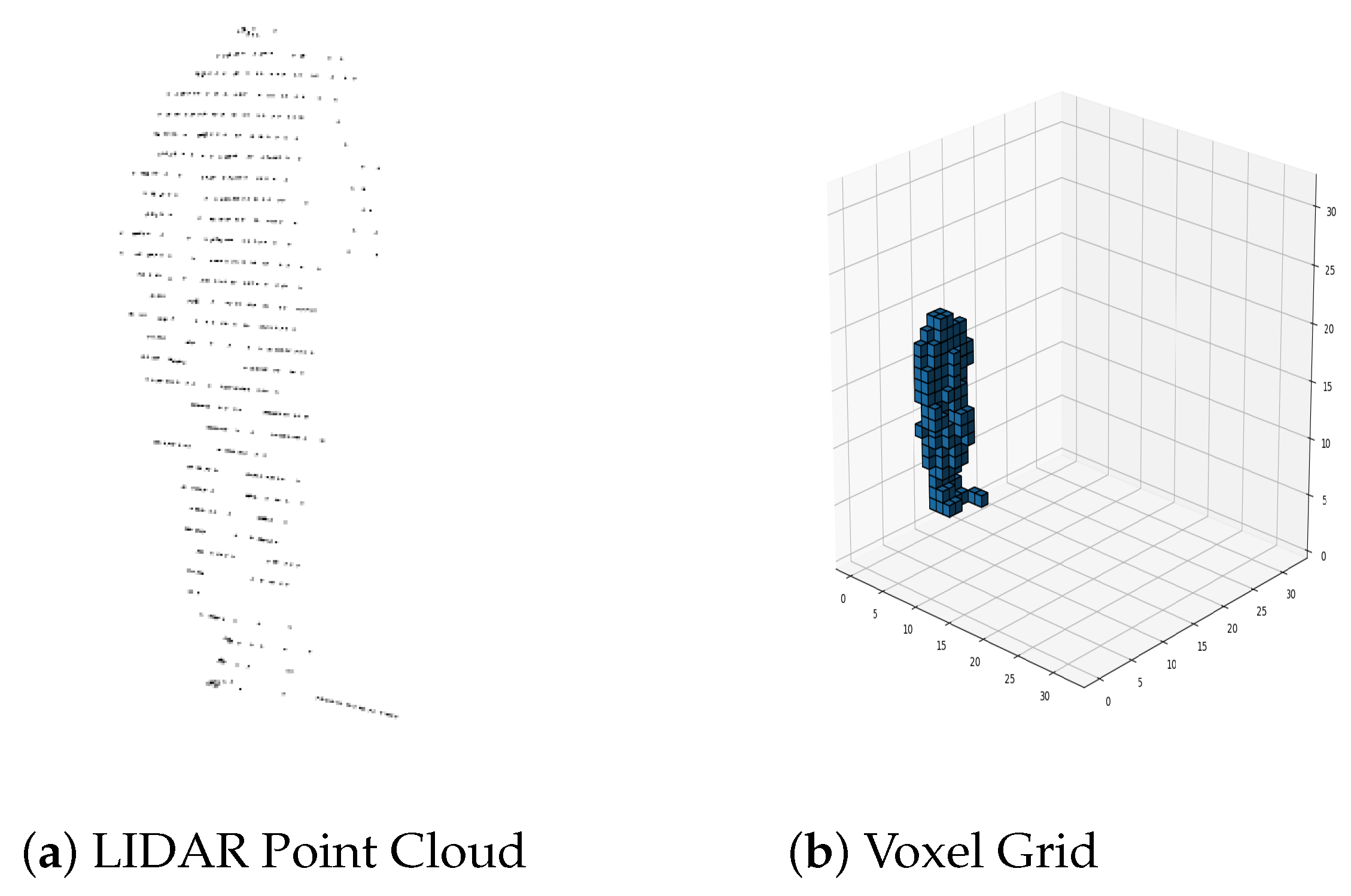
Figure 10.
Pedestrian extracted from a box: (a) Pedestrian as a LIDAR Point Cloud, (b) Pedestrian as a Voxel Grid.
Figure 10.
Pedestrian extracted from a box: (a) Pedestrian as a LIDAR Point Cloud, (b) Pedestrian as a Voxel Grid.
Figure 11.
Time performance and time per parameter for the SUOD neural network topology.
Figure 11.
Time performance and time per parameter for the SUOD neural network topology.
Table 1.
Hardware scheduler resources utilization.
Table 1.
Hardware scheduler resources utilization.
| Name | BRAM_18K | DSP48E | FF | LUT |
|---|
| Utilization | 260 | 6 | 4462 | 4867 |
Table 2.
Hardware neuron processing unit resources utilization.
Table 2.
Hardware neuron processing unit resources utilization.
| Name | BRAM_18K | DSP48E | FF | LUT |
|---|
| Utilization | 0 | 48 | 3623 | 6115 |
Table 3.
Accuracy for each dataset.
Table 3.
Accuracy for each dataset.
| Dataset | Tensorflow | 1 Core | 2 Cores | 3 Cores | 4 Cores |
|---|
| MNIST | 95.68% | 95.68% | 95.68% | 95.68% | 95.68% |
| Fashion MNIST | 87.05% | 87.05% | 87.05% | 87.05% | 87.05% |
| Cifar10 | 43.91% | 43.91% | 43.91% | 43.91% | 43.91% |
| Cifar100 | 14.01% | 14.01% | 14.01% | 14.01% | 14.01% |
Table 4.
Hardware “points to voxels” resources utilization.
Table 4.
Hardware “points to voxels” resources utilization.
| Name | BRAM_18K | DSP48E | FF | LUT |
|---|
| Utilization | 2 | 6 | 4043 | 7778 |
Table 5.
Results from hardware “points to voxels” module.
Table 5.
Results from hardware “points to voxels” module.
| Mean Box Size | Mean Execution Time | Mean Time per Point |
|---|
| 163 points | 880,240 ns | 5431 ns/point |
Table 6.
Accuracy results per dataset.
Table 6.
Accuracy results per dataset.
| Dataset | SUOD | 3D Point Cloud People Dataset |
|---|
| Accuracy | 37.22% | 93.99% |
| Publisher’s Note: MDPI stays neutral with regard to jurisdictional claims in published maps and institutional affiliations. |
© 2021 by the authors. Licensee MDPI, Basel, Switzerland. This article is an open access article distributed under the terms and conditions of the Creative Commons Attribution (CC BY) license (http://creativecommons.org/licenses/by/4.0/).


