Article

Utilizing B-Spline Curves and Neural Networks for Vehicle Trajectory Prediction in an Inverse Reinforcement Learning Framework

by
Mohammad Sadegh Jazayeri
and
Arash Jahangiri
*
Department of Civil, Construction, and Environmental Engineering, San Diego State University, 5500 Campanile Dr, San Diego, CA 92182, USA
*
Author to whom correspondence should be addressed.
J. Sens. Actuator Netw. 2022, 11(1), 14; https://0-doi-org.brum.beds.ac.uk/10.3390/jsan11010014
Submission received: 14 December 2021 / Revised: 20 January 2022 / Accepted: 5 February 2022 / Published: 10 February 2022
(This article belongs to the Special Issue Advances in Intelligent Transportation Systems (ITS))

Abstract

:
The ability to accurately predict vehicle trajectories is essential in infrastructure-based safety systems that aim to identify critical events such as near-crash situations and traffic violations. In a connected environment, important information about these critical events can be communicated to road users or the infrastructure to avoid or mitigate potential crashes. Intersections require special attention in this context because they are hotspots for crashes and involve numerous and complex interactions between road users. In this work, we developed an advanced machine learning method for trajectory prediction using B-spline curve representations of vehicle trajectories and inverse reinforcement learning (IRL). B-spline curves were used to represent vehicle trajectories; a neural network model was trained to predict the coefficients of these curves. A conditional variational autoencoder (CVAE) was used to generate candidate trajectories from these predicted coefficients. These candidate trajectories were then ranked according to a reward function that was obtained by training an IRL model on the (spline smoothed) vehicle trajectories and the surroundings of the vehicles. In our experiments we found that the neural network model outperformed a Kalman filter baseline and the addition of the IRL ranking module further improved the performance of the overall model.

1. Introduction

The problem of trajectory prediction involves forecasting the path a vehicle is going to take given its past trajectory and surroundings. A solution to this problem would have applications in surrogate safety analysis [1], evaluating road safety, and infrastructure-based safety systems for providing early crash warnings [2]. Solving this problem is also of critical importance for advanced driver assistance systems (ADAS) [3,4,5] and autonomous vehicles (AV) [3,6,7]. Solving this problem would also enable us to generate simulations of intersections that better conform to the reality of human driving. These more realistic simulations make it possible to predict the behavior of human drivers at intersections prior to their construction. This would allow for better safety assessments at intersections [8]. When cast as a control problem, i.e., a problem of finding the correct control behavior, solving the problem of trajectory prediction would be equivalent to training a model to drive similar to human drivers. This enables applications where human-like driving is desired. This problem is partly related to the problem of vehicle tracking, i.e., the problem of identifying and following the motion of vehicles in a video feed. While vehicle tracking deals with identifying the current motion of vehicles, trajectory prediction deals with predicting their future movements. The data required for trajectory prediction is the output of solving the vehicle tracking problem. In this work, we focused solely on the prediction problem.
Vehicle trajectory prediction is of particular interest at intersections, where a great number of conflicts between road users could increase the likelihood of accidents [9]. According to the National Traffic Safety Administration, between 2014 and 2018, about 40 percent of all crashes and 24 percent of fatal crashes occurred at intersections. With the advent of smart cities and smart vehicles, infrastructure to vehicle (I2V) and vehicle to vehicle (V2V) communications will be made possible. In conjunction with a trajectory prediction system, these advances in vehicle and infrastructure technology will enable us to enhance the safety of intersections by predicting collisions [10,11] and risky driving behavior [12] (e.g., red-light running) and deploying countermeasures to help avoid or mitigate crashes, such as early crash warnings [13,14,15,16,17], or real-time signal timing adjustments [18]. Being able to project vehicles’ trajectories into the future is also important in automated driving applications because, so long as automated vehicles share roads with human driven vehicles, they need to know how human drivers act in different situations and must also behave in ways that conform to human drivers’ expectation of other vehicles, i.e., similar to other human drivers. It is, therefore, important that automated vehicles have a model of vehicle motion in different situations including at intersections.
A wide range of approaches have been used in tackling the trajectory prediction problem, ranging in complexity from models that assume that the vehicle will maintain its velocity or acceleration and (rate of change of) heading for the duration for which trajectory prediction is going to be performed [19], to those that try to capture more of the complexities of vehicle motion by modeling different maneuvers, but that still disregard the influence of other vehicles [20], to models that take the interactions between traffic actors into account when predicting the future motion of vehicles [21]. The tools used in developing these approaches are also quite varied and include Kalman filters [15], hidden Markov models [22], Gaussian processes [20], Bayesian networks [14], Gaussian mixture models [9], and neural networks [6]. These studies all formulate the problem of trajectory prediction as a prediction task, which is to say that they directly predict the entire future trajectory of the vehicle; however, it can also be formulated indirectly as a control task in which control actions (e.g., changes in heading and velocity) are determined at each timestep and the trajectory can then be predicted by tracing the motion of the vehicle based on these actions. In this case, we will be dealing with a learning from demonstration (LfD) problem [23] in which we are interested in learning, from human driving data, what actions should be taken to properly control a vehicle.
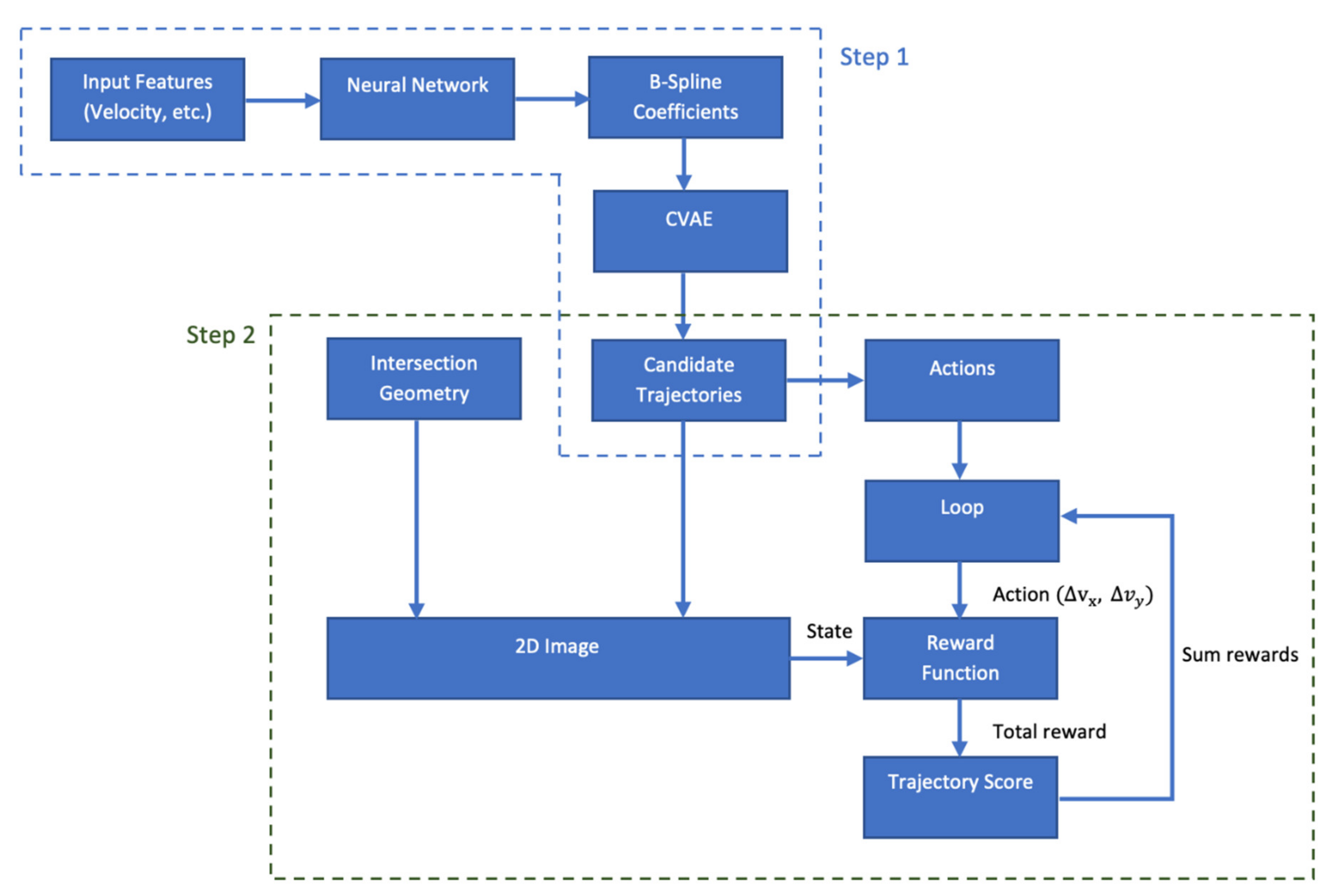
In this work, we developed a new solution using a hybrid approach combining elements from the prediction formulation and the control formulation based on a research project that we conducted [24]. We adopted a two-step approach to solving the problem. In the first step, we represented vehicle trajectories as B-spline curves and trained a neural network model to predict the coefficients of these B-spline curves. A conditional variational autoencoder was then used to generate candidate trajectories from these predicted coefficients. Similar approaches to trajectory representation have been used before, such as representing trajectories using Chebyshev polynomials [9]; but, to the best of our knowledge, this is the first work to use B-spline curves for this purpose. The reason why we chose B-spline curves for representing the trajectories is that B-spline curves can approximate complex curves with local control over the shape of the curve, while avoiding problems, such as oscillations at the edges of the interval (known as Runge’s phenomenon), that are encountered when using high degree polynomials. In the second step, the candidate trajectories were ranked using an inverse reinforcement learning (IRL) [25] model, in which a convolutional neural network was used as the approximator for the recovered reward function. IRL is a technique for solving control problems by learning from demonstration and has previously been used to solve the trajectory prediction problem in highways [26,27]; but, to the best of our knowledge, this is the first work to investigate its application to the problem at intersections. This is also the first work to use MaxEnt IRL to select from a set of candidate trajectories. The work in [28] also used an IRL-like approach to rank candidate trajectories, but used an ad hoc formulation. Trajectory prediction at intersections involves challenges not encountered in highways, such as the presence of various conflict types, multiple types of road users (vehicles, pedestrians, and bicycles), and more complicated traffic control devices. Here, we used IRL to develop methods that can address some of these complexities. The IRL model was trained using the B-spline smoothed trajectories and the context of the vehicle at the intersection, i.e., the other vehicles present at the intersection. The second step allowed us to predict trajectories that are more human-like and also to take interactions between the vehicles at the intersection into account. For the training and evaluation of our method we used the Lankershim boulevard dataset from the Next Generation Simulation (NGSIM) dataset collection [29]. In summary, the main contributions of this work are investigating (a) the use of B-spline curves to represent vehicle trajectories, (b) the use of inverse reinforcement learning in trajectory prediction at intersections, and (c) the use of MaxEnt IRL to rank a set of candidate trajectories.

2. Related Work

The approaches to trajectory prediction can be classified into three broad categories [3]: physics-based [10,13,15,19,30,31,32,33], maneuver-based [5,7,9,16,17,21], and interaction-aware [34,35,36,37]. Physics-based models, as the name suggests, deal with the physics of vehicle motion and assume that vehicles’ trajectories are determined solely by physical forces, disregarding driver decisions that affect steering and acceleration. Consequently, these models fail to accurately predict vehicle motion beyond a short horizon. Maneuver-based models take driver actions into account, but only in a vacuum, i.e., they consider these decisions to be determined solely by the position and the preceding trajectory of the vehicle of interest, ignoring the influence other road users have on these actions, which leads to less reliable projections of future motion. Interaction-aware models perform trajectory prediction by taking the presence of other road users into account. Comprehensive reviews of the three modeling approach categories can be found in [3,38]. The present work falls within the third category (i.e., interaction-aware models). What follows is a summary of interaction-aware models in the literature, previous studies that have applied IRL to the problem of trajectory prediction, and works that involve the application of trajectory prediction to intersection safety.

2.1. Interaction-Aware Models

In [34], a trajectory prediction framework based on a radial basis function (RBF) network and particle filter proposed in [5] was used to predict the joint trajectory of two vehicles at intersections. This was performed by penalizing those trajectories that lead to avoidable collisions (i.e., trajectories for which the time to collision is larger than the drivers’ reaction times). Coupled hidden Markov models [22] were used in [21] with the assumption of asymmetric interactions, i.e., other vehicles influence the vehicle of interest, but not vice versa, to predict driver behavior. In [35], the intelligent driver model was used to infer the intent of drivers at intersections in the presence of a preceding vehicle. A probabilistic graphical model and recursive Bayesian filtering were used in [36,39] to perform interaction-aware driving behavior prediction. In [37], a dynamic Bayesian network (DBN) was used in conjunction with a factored state space that allows for a model with less computational complexity. DBNs were also used in [40] to jointly model what drivers intend to do and what they are expected to do in a traffic context. In [6], traffic contexts were rasterized into two dimensional images and a deep convolutional neural network was then used to perform trajectory prediction. In [41], a generative adversarial network (GAN) was used to model driver behavior in highways. A solution to a restricted version of the trajectory prediction problem, that of predicting the changes in velocity along a predetermined path at unsignalized intersections, was proposed in [42]. This work modeled the problem as a partially observable Markov decision process in which the intended path of the other vehicles constitute the hidden variables. Partially observable Markov decision processes were also used in [43] for AV decision making in scenarios, including roundabouts and T junctions. In [44], deep neural networks (DNNs) and long short term memory (LSTM) networks were used to predict vehicle trajectories at intersections. A technique called social pooling was used with LSTM and deep CNNs in [45] to address the interactions between vehicles in trajectory prediction in a highway setting. In [46], a specially designed “influence network” was used in conjunction with a DBN to perform vehicle trajectory prediction at intersections. A similar solution to the trajectory prediction problem based on DBNs was proposed in [14].

2.2. Trajectory Prediction Using IRL

Several studies have used IRL to model driving, mostly in the context of highways. In [26], IRL was used to learn driving in highways from human demonstrations in a simulated environment. The use of IRL was motivated by the desire to achieve more humanlike behavior and a better ability to handle new scenarios. Deep Q-networks were used to address the exploding state space issue encountered in using IRL in a setting with a large state space. In addition to using a simulated environment instead of real-world data, this study contained several other limitations, such as using constant speed and having at most two cars in front of the vehicle. The authors in [27] had similar motivations in using IRL for the task of learning individual driving styles on highways. The driving behavior of a number of drivers was recorded as they drove a car fitted with a variety of sensors on a highway. Maximum entropy IRL was then used to train a model to make driving decisions in styles similar to each of the individual drivers. This work used a reward function that was a linear function of a number of manually defined features such as acceleration, deviation from lane center, and distance to other vehicles. These last two works considered the control problem that was mentioned earlier in the introduction section. In both studies, the use of IRL allowed for faithful replication of human driving behavior and an ability to generalize to new situations. In [47], a hierarchical learning framework was proposed, in which IRL was used to predict interactive driving behavior on two levels with a case study of ramp merging. The different levels of decision making in their framework consisted of discrete, high-level decisions (e.g., whether to merge after or before a given car in their case study) and low-level continuous actions (e.g., the acceleration and heading changes at each timestep.) Similar to the previous study, the reward function in this work was formulated as a linear function of several manually defined features. A notable limitation of this work is that the high-level discrete decisions and their corresponding low-level continuous features need to be manually defined based on the particular scenario (e.g., ramp merging) at hand. In [28], a generative framework based on conditional variational autoencoders using recurrent neural networks was used to generate possible future trajectories. An IRL approach was used to rank and refine the trajectories generated by the generative framework. It is noteworthy that this work did not use any of the commonly employed IRL formulation, but rather integrated a reward function into a larger framework, where the reward function parameters were optimized in tandem with the rest of the architecture and the optimization method was dependent upon the sample generating component of the framework. IRL was used in [48] to choose from a set of trajectories generated using a rule-based method in a highway environment. IRL was chosen as the approach for this study because it allowed for a hybrid method that did not require mappings from circumstances to vehicle control to be manually engineered and, at the same time, produced interpretable results. In [49], a trajectory prediction method based on an encoder-decoder approach using RNNs was proposed, which used IRL as a regularizer for the training of the encoder-decoder network. The use of IRL as a regularizer was intended to help the model better utilize the scene context information. IRL was used to directly predict trajectories in a highway environment in [50]. A summary of the studies enumerated above is presented in Table 1.

2.3. Trajectory Prediction for Intersection Safety

In this subsection, we will explore in more detail those studies that have considered the trajectory prediction problem from the viewpoint of the infrastructure and whose proposed solutions cover the problem at intersections.
Trajectory prediction has several applications for intersection safety. One such application is the detection of risky driving behaviors such as dangerous turns [16], red-light running [12,16,18], abrupt stops, aggressive passes, speeding passes, and aggressive following [12]. Trajectory prediction is also instrumental to the early prediction of turning movements, which is helpful in avoiding accidents [43]. Collision prediction, avoidance/mitigation [13,14,15,19], and risk assessment [10,11,17] also make use of trajectory prediction. Each of the studies reviewed in this subsection used their solutions to the problem of trajectory prediction to tackle one or more of these applications. Table 2 presents, for each study, the features used for trajectory prediction (Predictors), the sensors used for collecting these features’ data (Data Collection Sensors), the number of intersections where data were gathered for training (if applicable), the duration for which data needed to be collected before starting to make predictions (monitoring period), how far into the future the predicted trajectories stretch (prediction horizon), what evaluation metric was used for measuring the performance of either the trajectory prediction method, or the safety system as a whole (evaluation metric), the applications that were tested if applicable (tested applications), interactions between which types of road users were considered (interaction type), and what movements leading to possible hazards were considered.
Most studies have focused on predicting and mitigating crashes. In [10], the authors proposed a method for collision risk estimation between vehicles based on real time trajectory prediction. The method used for trajectory prediction in this work was a linear Kalman filter. GPS data was used for determining the position of vehicles, and risk estimation was performed using the time to collision (TTC) predicted from the predicted trajectories. Another work to use TTC from predicted trajectories for collision risk estimation was [13], which also used a Kalman filter for trajectory prediction and DGPS as the position sensor. A system for threat assessment and decision-making system was proposed in [15], which used an unscented Kalman filter for trajectory prediction. A probabilistic threat assessment method was also developed for threat assessment, along with a decision-making protocol for whether an intervention is necessary. In [14], an accident prewarning system was developed with a trajectory prediction method based on a DBN and a risk assessment method based on the identification of risky driving behavior. They also presented a method for deciding the collision avoidance strategy that is based on TTC and time to avoidance (TTA) matrices. An intersection safety system was developed in [11], which used video data to predict the trajectory of vehicles at intersections and to detect dangerous situations involving both vehicles and pedestrians using TTC and post encroachment time (PET). For trajectory prediction, it was assumed that vehicles drive according to “average drive lines,” which were predefined average trajectories for vehicles. In [17], a trajectory prediction method based on extended Kalman filters was developed and used to identify conflict areas between vehicles and other road users and calculate time to enter (TTE) and time to leave (TTL) for these road users and conflict areas. An object-oriented Bayesian network was then used to estimate collision probability. In [16], a maneuver prediction model was presented for use in an infrastructure-based intersection safety system. The proposed system used location, speed, and acceleration data transmitted by vehicles and roadside sensors for maneuver prediction. The objective of the system was to provide warnings for red-light violations and right and left turning hazards.
There are also other studies that have focused on other applications such as the identification of certain behaviors. In [12], the authors developed a trajectory prediction method for identifying risky behavior at high-speed intersections that are caused by the lengthy warning sequence at the end of the green phase at these intersections. A notable feature of their method is that it divides the problem into two cases: the case where the vehicle has enough distance from its leading vehicle that it acts independently of it, and the case where the vehicle’s movements are influenced by the behavior of the leading vehicle (i.e., time headway to the leading vehicle is less than 6 s). A trajectory prediction method was developed in [44] for predicting turning movements at intersections. Video data from three intersections was used to extract vehicle trajectories and to train neural network models for predicting vehicle trajectories. In the process of predicting the turning movement of the vehicles, after a vehicle’s trajectory has been predicted, it is compared against “typical paths” in order to obtain the final turning prediction (left, right, or through). In [46], trajectory data transcribed from a video camera was used to train neural network models for trajectory prediction of both vehicles and pedestrians, which can be used for predicting high level behavior. A red-light running prediction method was proposed in [18], which used trajectory prediction to detect red-light running ahead of time and dynamically extend the all-red phase of the intersection signals to mitigate accidents. A method for collision risk prediction and warning was proposed in [19], which estimated the minimal future distance between possibly conflicting vehicles using a physics-based trajectory prediction method.

3. Materials and Methods

3.1. Data Description

For this study we used the Lankershim Boulevard dataset from the Next Generation Simulation (NGSIM) dataset collection. This dataset contains vehicle trajectories transcribed from video data providing complete coverage of three signalized intersections and covering approximately 500 m in length. The dataset comprises a total of 30 min of data starting from 8:15 a.m. These 30 min of data cover a wide range of traffic conditions at the intersections including the intersection being nearly empty and the intersections being heavily populated by vehicles. The data is in a tabular format with each row corresponding to the state of a specific vehicle at a specific time. The data is sampled at 10 Hz and contains the vehicle’s position, lane number, velocity, acceleration, and the intersection at which it is currently located among its columns. In addition to trajectory data, this dataset also contains street marking data.

Data Cleaning and Organization

The trajectory data in the NGSIM dataset is provided as a single tabular file (in csv format) that provides data on the location (in latitude and longitude based both on the CA state plane III and also locally relative to the center of the boulevard in feet), type (auto/truck/motorcycle), speed (in feet per second), and size (length and width in feet) of each vehicle at each point in time. A new column was added to the data to indicate whether each row corresponds to a vehicle being in the area of influence of an intersection and, if so, which one. This new column was used to remove the data pertaining to the times when vehicles were outside the intersection’s area of influence. A vehicle was considered to be within an intersection’s area of influence if it was no more than 60 m away from the closest edge of the intersection; the 60-m threshold was chosen so as to correspond with the length of the longest monitoring period that we wanted to consider. Moreover, the rows belonging to each vehicle were grouped and sorted with respect to time in order to obtain the vehicle trajectories. We also calculated the heading (in radians) for each vehicle at each point in time and added it as a column. Finally, the trajectories were rotated and translated such that their point of entry into the intersection was at the origin of the plane; straight movement through the intersection corresponded to movement along the y axis. Table 3 provides an overview of the statistics of the dataset.

3.2. Methodology

Our method is made up of two steps: In the first step, B-spline curves were fit to vehicle trajectories in order to represent each vehicle trajectory using the coefficients of the B-splines. A neural network was then trained to predict these coefficients. The B-spline coefficients were also used to train a conditional variational autoencoder that was used to generate candidate trajectories from the predicted coefficients. In the second step, the B-spline smoothed trajectories of the vehicles were embedded into images containing the geometry of the intersection and the other vehicles present at the intersection. These images were then used to train an IRL model, which we used for evaluating the candidate trajectories and choosing the best among them. Figure 1 provides an overview of our method. In the following two subsections, we provide an overview of B-spline curves and IRL.

3.2.1. B-Splines

For a given knot sequence t 0 t 1 t n + d + 1 the B-spline basis functions are defined recursively as follows:
N i , 0 t = 1 ,     t i t t i + 1 0 ,     o t h e r w i s e
N i , j t = t t i t i + j t i N i , j 1 t + t i + j + 1 t t i + j + 1 t i + 1 N i + 1 , j 1 t
where 1   j   d and 0   i   n + d j . A one-dimensional B-spline curve is then defined in the following way:
x t = i = 0 n c i N i , d t
For a given knot sequence and value of d , the c i s uniquely determine f t and are referred to as the spline coefficients. In the training phase, these coefficients are estimated by finding the values of c i that minimize the following objective function:
t x t i = 0 n c i N i , d t
In the test phase, these coefficients are predicted by a neural network and the corresponding B-spline curve is the predicted trajectory. Note that we used univariate splines, which means that, in order to represent each trajectory, we needed two spline curves, x t and y t , corresponding to the x and y coordinates of the trajectory, respectively.

3.2.2. Conditional Variational Autoencoders

A conditional variational autoencoder (CVAE) [51] is a generative model based on variational autoencoders (VAEs) [52] that allows us to model and generate samples from a distribution conditioned on some input variable(s). A CVAE is made up of an encoder Q z | X , c mapping the input, X , to gaussian latent variables with the help of the conditioning variable(s) c and a decoder P ( X | z ,   c ) mapping the latent variables back to the input space with the help of the conditioning variables. Here, we have used a CVAE to generate trajectories similar to a given initial trajectory by letting c = X . This results in Q ( z | X , c ) = Q ( z | X ) .

3.2.3. Inverse Reinforcement Learning

The Reinforcement Learning (RL) Problem

The RL problem involves learning what actions to take in an interactive environment to maximize an objective function (called reward). The main elements of reinforcement learning are the decision-making entity called the agent, the environment with which the agent interacts, and a reward signal, which is a numerical value provided by the environment to the agent at each timestep. The goal of the agent is to maximize the sum of the reward it receives over time.
Formally, an RL problem is defined by a Markov decision process (MDP.) An MDP is a tuple S ,   A ,   p ,   γ ,   r , in which S is the set of all the states that the environment can be in, A is the set of actions the agent can take, p s | s ,   a is the probability of the environment transitioning from state s to state s if the agent takes action a , γ is the discount factor, and r s ,   a ,   s is the expected reward given to the agent when the environment transitions from state s to state s after the agent has taken action a . A policy π a | s defines the probability of the agent taking action a when in state s . The expected return for a state s under a given policy π is the expected sum of the discounted reward values received by an agent starting from s and making decision based on π and is denoted by v π s , leading to v π s = a π a | s s p s | s ,   a [ r s ,   a ,   s + γ v π s ] . In reinforcement learning, the objective is to find the optimal policy π * which maximizes v π * s for every state s .

The Inverse Reinforcement Learning (IRL) Problem

While the RL problem involves finding an optimal policy given a reward function, the IRL problem involves finding a reward function for which a given policy (represented by a set of samples from expert demonstrations) is optimal. Finding this reward function allows us to derive the policy and reproduce the behavior of the expert. The IRL problem as stated is ill-posed, because there are multiple reward functions for which a given policy is optimal; for instance, the set of reward functions that are constant everywhere are optimal for every policy. There have been several approaches to addressing this issue, one of which is the maximum entropy formulation [53]. In this formulation, it is assumed that the probability of a specific sequence of states and actions (denoted by τ ) being observed is equal to p τ = 1 Z exp r θ τ , in which r θ τ = s , a τ r θ s ,   a , where r θ is the reward function parametrized by θ . This formulation posits that the expert acts probabilistically and is most likely to traverse the optimal sequence of actions and states, with suboptimal sequences being exponentially less probable as their associated reward decreases. The central problem in this formulation is calculating or estimating the value of Z (often called the partition function). Several approaches have been proposed for solving this problem. In guided cost learning [54] (GCL), the algorithm we used, this is achieved by importance sampling from the set of all possible sequences of states and actions. This importance sampling involves generating samples not present in the dataset. This is explored in more detail in the “Results and Discussion” section of this paper. The reason for choosing GCL here is that it enables tractably working with high dimensional and continuous state spaces and actions, while allowing for a nonlinear function approximator (here, a neural network) to be used for approximating the reward function.
In our method, we used GCL with a convolutional neural network as the approximator for the reward function to recover the reward function of the human drivers and then used the recovered reward function to rank the candidate trajectories generated in the first step of the method. To this end, we first needed to convert each candidate trajectory to a sequence of states and actions. The state at time t was specified by creating a 2D image of the intersection containing the intersection geometry and the trajectories of all the vehicles at the intersection up to time t . The action at time t was a two-dimensional value specifying the change in velocity of the vehicle in the x and y directions at time t . If we denote the recovered reward function with r s t , a t , in which s t denotes the state at time t and a t = Δ v x , Δ v y t is the ordered pair representing the action at time t , the score, denoted by u , assigned to a trajectory τ = s 1 , a 1 , , s n , a n is calculated using the following:
u = t = 1 n r s t , a t
The value of u was calculated for every candidate trajectory and the candidate trajectory with the highest value was chosen as the final predicted trajectory.
The asymptotic computational complexity of the prediction algorithm is as follows:
θ c f t
where c is the number of candidate trajectories, f is the resolution (in hertz) at which the simulation for the second step is performed, and t is the prediction horizon (in seconds). It should be noted that the processing required for the prediction algorithm is highly parallelizable: candidate trajectories can be scored independently and, in scoring a trajectory, every iteration of the loop in Figure 1. is independent of every other; thus, the loop can be completely parallelized.

4. Results and Discussion

In our experiments, we used the Lankershim Boulevard data from the NGSIM dataset. We extracted vehicle trajectories from this data and fit B-spline curves to the extracted trajectories. Of the resulting data, 10% was set aside as test data (distributed uniformly over the three different movement types). We then trained a neural network to predict the coefficients of the B-spline curves corresponding to the trajectories using 10-fold cross validation on the rest of the data. The neural network had the following input features: the x and y distance from the center of the approach from which the vehicle entered the intersection to the centers of the three road segments by which the vehicle can exit the intersection, the distance of the vehicle from the center of the approach, velocity before entering the intersection, vehicle acceleration before entering the intersection, vehicle heading before entering the intersection, average vehicle velocity over the monitoring period (2 s in the final model), average vehicle acceleration over the monitoring period, and the turning movements allowed for the lane that the vehicle was in. We then generated candidate trajectories by randomly perturbing the predicted coefficients. An IRL model was trained in the following manner: the B-spline smoothed trajectories of the vehicles were embedded into images containing the geometry of the intersection, as well as the trajectories of the other vehicles present at the intersection (at test time, the trajectories predicted in the first step were used.) For the reward function approximator, we used a pretrained convolutional neural network, namely MobileNetV2, with the final softmax layer removed. As noted in the “Methods” section, training an IRL model using the GCL algorithm involved sample generation. This was done by changing the trajectory of the ego vehicle with respect to the sampled actions while maintaining the original trajectory of other vehicles. The trained IRL model gave us a recovered reward function that was subsequently used to score the candidate trajectories generated in the first step of the algorithm. The candidate trajectory scoring the highest was the final prediction of the model.
The results of our experiments are summarized in Table 4. We see that the first step of our method without ranking by the IRL module already outperformed the baseline model. The addition of the IRL module further improved the performance of the model. Most of the works reviewed in the “Related Works” section either did not provide quantitative results of their methods or reported metrics on downstream tasks only. Of those that reported performance on the trajectory prediction task, none reported results on the same dataset as ours. However, to give a point of comparison, we have included results from two studies that reported results from comparable experiments.
For a qualitative assessment of the performance of the model, we can consider the trajectories in Figure 2. Here, we have the ground truth trajectory of a left turn in blue with the prediction of the first step in red and, finally, the trajectory assigned the highest score by the IRL method in green. We can observe that the trajectory selected by the IRL module is not only closer in location to the ground truth trajectory, but also more similar to it in shape and direction.
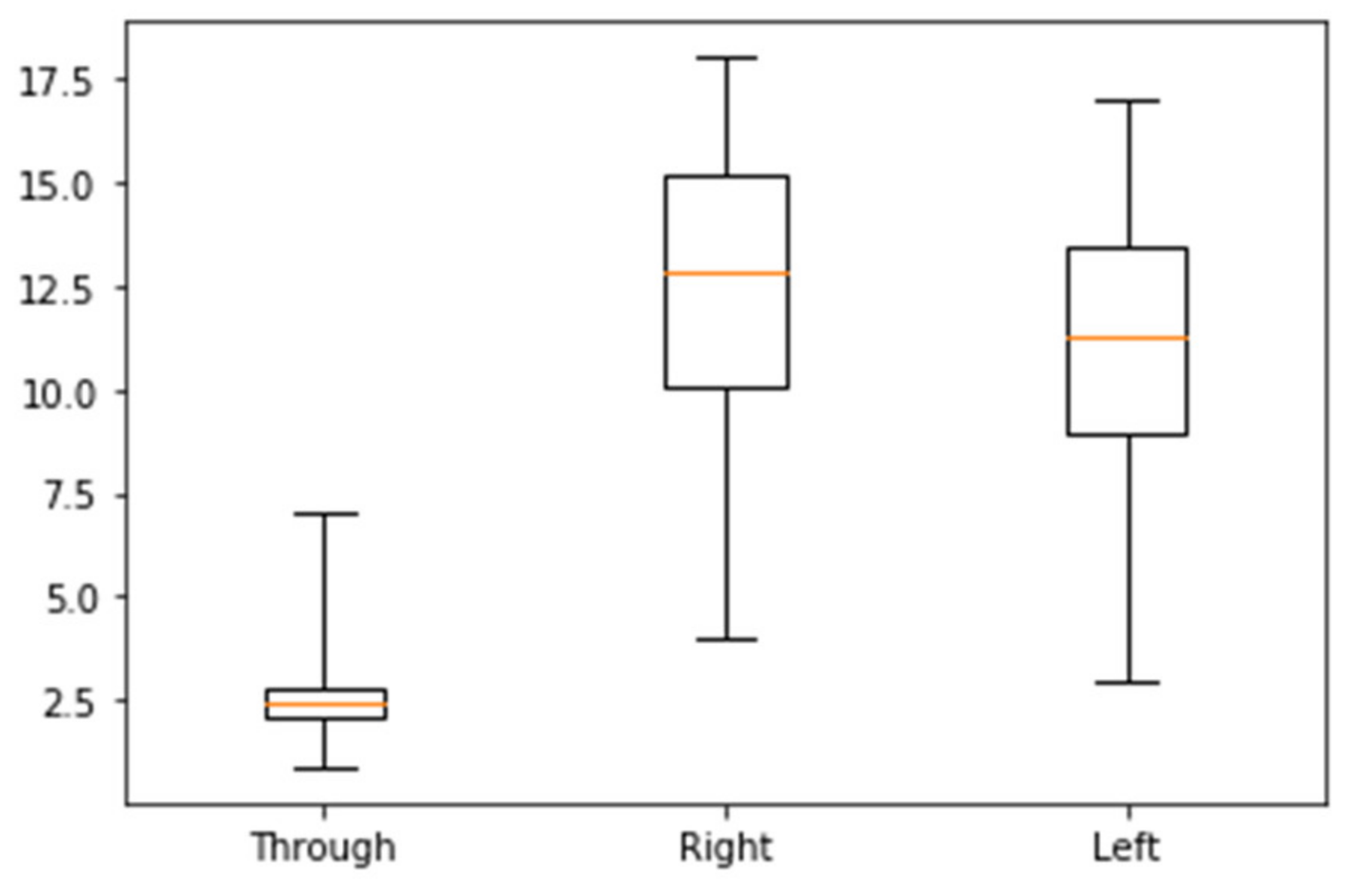
To better understand the performance of the model, as well as the way in which the IRL module improves predictions, we consider the errors of the models broken down by movement type, i.e., whether the vehicle in question was going through the intersection, turning right, or turning left. The error values for different movement types are reported in Table 5, showing that the effect of the IRL scoring module is more pronounced in predicting turning movements. This can be explained by the fact that predicting the trajectory of turning movements is more difficult; the IRL scoring module is, therefore, more likely to find a better trajectory among the generated candidates and return it as the top scoring trajectory. In Figure 3, we can see a boxplot of the RMSE values by movement.
We can also look at the error of the models as a function of the prediction horizon. These figures are reported in Table 6. We again notice that, as the task gets more difficult, the impact of the IRL scoring module increases. Here, we see that the further the prediction horizon is, the more the IRL scoring module is able to improve predictions. This can be explained in the same way as the previous observation with through and turning movements: as the trajectories get more difficult to predict, the IRL scoring module is more likely to select a trajectory that is considerably more accurate from the set of candidate trajectories.

5. Conclusions

Here, we have presented a two-step method for vehicle trajectory prediction at intersections. The first step of our method involved representing vehicle trajectories using B-spline curves, training a neural network to predict the coefficients of these B-spline curves, and the use of a conditional variational autoencoder to generated candidate trajectories from these predicted B-spline coefficients. The second step of our method consisted of using a reward function recovered by training an IRL model to the data to score these candidate trajectories and produce the final prediction. We have shown that a hybrid approach mixing elements from conventional supervised methods with elements from imitation learning can yield viable results for trajectory prediction. Our results indicate that IRL is an effective tool for addressing the shortcomings of conventional supervised methods with regard to the problem of trajectory prediction. We have, furthermore, demonstrated the suitability of B-spline curves for representing vehicle trajectories in such a way as to enable prediction. An avenue for future work lies in making context information available to the first step of the method. By making the model aware of interactions between vehicles from the first step, it should be possible to provide better input to the IRL scoring module and to further improve the accuracy of the overall model. Another possible area for improvement would be modifications that allow the model to provide predictions before or after the vehicle reaches the intersection, i.e., flexibility in terms of the starting point of the prediction. The performance of the model could also benefit from improvements to the architecture of the neural networks used. In the current work the architecture of the neural networks was determined by manual iteration; in future work, this can be better accomplished by using neural architecture search [55]. Finally, investigating the practicality of the developed methodology in solving downstream tasks (e.g., collision prediction) is a logical next step.

Author Contributions

Conceptualization, A.J. and M.S.J.; methodology, M.S.J. and A.J.; validation, M.S.J.; formal analysis, M.S.J. and A.J.; investigation, M.S.J. and A.J; resources, A.J.; data curation, M.S.J.; writing—original draft preparation, M.S.J. and A.J; writing—review and editing, M.S.J. and A.J.; visualization, M.S.J.; supervision, A.J.; project administration, A.J.; funding acquisition, A.J. All authors have read and agreed to the published version of the manuscript.

Funding

This research was funded by the Safety through Disruption (Safe-D) National University Transportation Center (UTC), a grant from the U.S. Department of Transportation’s University Transportation Centers Program (Federal Grant Number: 69A3551747115). The contents of this paper reflect the views of the authors, who are responsible for the facts and the accuracy of the information presented herein.

Institutional Review Board Statement

Not applicable.

Informed Consent Statement

Not applicable.

Data Availability Statement

Conflicts of Interest

The authors declare no conflict of interest.

References

  1. Mohamed, M.G.; Saunier, N. Motion Prediction Methods for Surrogate Safety Analysis. Transp. Res. Rec. 2013, 2386, 168–178. [Google Scholar] [CrossRef]
  2. Wolterman, M. Infrastructure-Based Collision Warning Using Artificial Intelligence. U.S. Patent 7,317,406 B2, 8 January 2008. [Google Scholar]
  3. Lefèvre, S.; Vasquez, D.; Laugier, C. A Survey on Motion Prediction and Risk Assessment for Intelligent Vehicles. ROBOMECH J. 2014, 1, 1. [Google Scholar] [CrossRef] [Green Version]
  4. Schreier, M.; Willert, V.; Adamy, J. An Integrated Approach to Maneuver-Based Trajectory Prediction and Criticality Assessment in Arbitrary Road Environments. IEEE Trans. Intell. Transport. Syst. 2016, 17, 2751–2766. [Google Scholar] [CrossRef]
  5. Hermes, C.; Wohler, C.; Schenk, K.; Kummert, F. Long-Term Vehicle Motion Prediction. In Proceedings of the 2009 IEEE Intelligent Vehicles Symposium, Xi’an, China, 3–5 June 2009; pp. 652–657. [Google Scholar]
  6. Djuric, N.; Radosavljevic, V.; Cui, H.; Nguyen, T.; Chou, F.-C.; Lin, T.-H.; Schneider, J. Motion Prediction of Traffic Actors for Autonomous Driving Using Deep Convolutional Networks. arXiv 2018, arXiv:1808.05819. [Google Scholar]
  7. Vasquez, D.; Fraichard, T.; Laugier, C. Growing Hidden Markov Models: An Incremental Tool for Learning and Predicting Human and Vehicle Motion. Int. J. Robot. Res. 2009, 28, 1486–1506. [Google Scholar] [CrossRef] [Green Version]
  8. Gettman, D.; Head, L. Surrogate Safety Measures from Traffic Simulation Models. Transp. Res. Rec. 2003, 1840, 104–115. [Google Scholar] [CrossRef] [Green Version]
  9. Wiest, J.; Höffken, M.; Kreßel, U.; Dietmayer, K. Probabilistic Trajectory Prediction with Gaussian Mixture Models. In Proceedings of the 2012 IEEE Intelligent Vehicles Symposium, Madrid, Spain, 3–7 June 2012; pp. 141–146. [Google Scholar]
  10. Ammoun, S.; Nashashibi, F. Real Time Trajectory Prediction for Collision Risk Estimation between Vehicles. In Proceedings of the 2009 IEEE 5th International Conference on Intelligent Computer Communication and Processing, Cluj-Napoca, Romania, 27–29 August 2009; pp. 417–422. [Google Scholar]
  11. Pyykönen, P.; Molinier, M.; Klunder, G.A. Traffic Monitoring and Modeling for Intersection Safety. In Proceedings of the 2010 IEEE 6th International Conference on Intelligent Computer Communication and Processing, Cluj-Napoca, Romania, 26–28 August 2010; pp. 401–408. [Google Scholar]
  12. Tan, C.; Zhou, N.; Wang, F.; Tang, K.; Ji, Y. Real-Time Prediction of Vehicle Trajectories for Proactively Identifying Risky Driving Behaviors at High-Speed Intersections. Transp. Res. Rec. 2018, 2672, 233–244. [Google Scholar] [CrossRef]
  13. Wang, Y.; Wenjuan, E.; Tian, D.; Lu, G.; Yu, G.; Wang, Y. Vehicle Collision Warning System and Collision Detection Algorithm Based on Vehicle Infrastructure Integration. In Proceedings of the 7th Advanced Forum on Transportation of China (AFTC 2011), Beijing, China, 22 October 2011; pp. 216–220. [Google Scholar]
  14. Fu, Y.; Li, C.; Luan, T.H.; Zhang, Y.; Mao, G. Infrastructure-Cooperative Algorithm for Effective Intersection Collision Avoidance. Transp. Res. Part C Emerg. Technol. 2018, 89, 188–204. [Google Scholar] [CrossRef]
  15. De Campos, G.R.; Runarsson, A.H.; Granum, F.; Falcone, P.; Alenljung, K. Collision Avoidance at Intersections: A Probabilistic Threat-Assessment and Decision-Making System for Safety Interventions. In Proceedings of the 17th International IEEE Conference on Intelligent Transportation Systems (ITSC), Qingdao, China, 8–11 October 2014; pp. 649–654. [Google Scholar]
  16. Schendzielorz, T.; Mathias, P.; Busch, F. Infrastructure-Based Vehicle Maneuver Estimation at Urban Intersections. In Proceedings of the 16th International IEEE Conference on Intelligent Transportation Systems (ITSC 2013), The Hague, The Netherlands, 6–9 October 2013; pp. 1442–1447. [Google Scholar]
  17. Weidl, G.; Breuel, G.; Singhal, V. Collision Risk Prediction and Warning at Road Intersections Using an Object Oriented Bayesian Network. In Proceedings of the 5th International Conference on Automotive User Interfaces and Interactive Vehicular Applications—AutomotiveUI ’13, Eindhoven, The Netherlands, 28–30 October 2013; ACM Press: New York, NY, USA, 2013; pp. 270–277. [Google Scholar]
  18. Wang, L.; Zhang, L.; Zhang, W.-B.; Zhou, K. Red Light Running Prediction for Dynamic All-Red Extension at Signalized Intersection. In Proceedings of the 2009 12th International IEEE Conference on Intelligent Transportation Systems, St. Louis, MO, USA, 4–7 October 2009; pp. 1–5. [Google Scholar]
  19. Wang, P.; Chan, C.-Y. Vehicle Collision Prediction at Intersections Based on Comparison of Minimal Distance between Vehicles and Dynamic Thresholds. IET Intell. Transp. Syst. 2017, 11, 676–684. [Google Scholar] [CrossRef]
  20. Tran, Q.; Firl, J. Online Maneuver Recognition and Multimodal Trajectory Prediction for Intersection Assistance Using Non-Parametric Regression. In Proceedings of the 2014 IEEE Intelligent Vehicles Symposium Proceedings, Dearborn, MI, USA, 8–11 June 2014; pp. 918–923. [Google Scholar]
  21. Oliver, N.; Pentland, A.P. Graphical Models for Driver Behavior Recognition in a SmartCar. In Proceedings of the IEEE Intelligent Vehicles Symposium 2000 (Cat. No.00TH8511), Dearborn, MI, USA, 5 October 2000; pp. 7–12. [Google Scholar]
  22. Brand, M.; Oliver, N.; Pentland, A. Coupled Hidden Markov Models for Complex Action Recognition. In Proceedings of the IEEE Computer Society Conference on Computer Vision and Pattern Recognition, San Juan, PR, USA, 17–19 June 1997; pp. 994–999. [Google Scholar]
  23. Schaal, S. Learning from Demonstration. In Advances in Neural Information Processing Systems 9; Mozer, M.C., Jordan, M.I., Petsche, T., Eds.; MIT Press: Cambridge, MA, USA, 1997; pp. 1040–1046. [Google Scholar]
  24. Jazayeri, M.S.; Jahangiri, A.; Machiani, S.G. Predicting Vehicle Trajectories at Intersections Using Advanced Machine Learning Techniques; SAFE-D, Safety Through Disruption National University Transportation Center: San Diego, CA, USA, 2021. [Google Scholar]
  25. Russell, S.J. Learning Agents for Uncertain Environments. In Proceedings of the 11th Annual Conference on Computational Learning Theroy, Madison, WI, USA, 24–26 July 1998; Volume 98, pp. 101–103. [Google Scholar]
  26. Sharifzadeh, S.; Chiotellis, I.; Triebel, R.; Cremers, D. Learning to Drive Using Inverse Reinforcement Learning and Deep Q-Networks. arXiv 2016, arXiv:1612.03653. [Google Scholar]
  27. Kuderer, M.; Gulati, S.; Burgard, W. Learning Driving Styles for Autonomous Vehicles from Demonstration. In Proceedings of the 2015 IEEE International Conference on Robotics and Automation (ICRA), Seattle, WA, USA, 26–30 May 2015; pp. 2641–2646. [Google Scholar]
  28. Lee, N.; Choi, W.; Vernaza, P.; Choy, C.B.; Torr, P.H.S.; Chandraker, M. DESIRE: Distant Future Prediction in Dynamic Scenes with Interacting Agents. In Proceedings of the 2017 IEEE Conference on Computer Vision and Pattern Recognition (CVPR), Honolulu, HI, USA, 21–26 July 2017; pp. 2165–2174. [Google Scholar]
  29. Kovvali, V.; Alexiadis, V.; Zhang, L. Video-Based Vehicle Trajectory Data Collection (No. 07-0528). In Proceedings of the Transportation Research Board 86th Annual Meeting, Washington, DC, USA, 21–25 January 2007. [Google Scholar]
  30. Lin, C.-F.; Ulsoy, A.G.; LeBlanc, D.J. Vehicle Dynamics and External Disturbance Estimation for Vehicle Path Prediction. IEEE Trans. Control Syst. Technol. 2000, 8, 508–518. [Google Scholar] [CrossRef]
  31. Barth, A.; Franke, U. Where Will the Oncoming Vehicle Be the next Second? In Proceedings of the 2008 IEEE Intelligent Vehicles Symposium, Eindhoven, The Netherlands, 4–6 June 2008; pp. 1068–1073. [Google Scholar]
  32. Veeraraghavan, H.; Papanikolopoulos, N.; Schrater, P. Deterministic Sampling-Based Switching Kalman Filtering for Vehicle Tracking. In Proceedings of the 2006 IEEE Intelligent Transportation Systems Conference, Toronto, ON, Canada, 17–20 September 2006; pp. 1340–1345. [Google Scholar]
  33. Shao, Q.B.; Guan, H.; Jia, X. Vehicle Trajectory Prediction Based on Road Recognition. Appl. Mech. Mater. 2014, 599, 760–766. [Google Scholar] [CrossRef]
  34. Käfer, E.; Hermes, C.; Wöhler, C.; Ritter, H.; Kummert, F. Recognition of Situation Classes at Road Intersections. In Proceedings of the 2010 IEEE International Conference on Robotics and Automation, Anchorage, AK, USA, 3–7 May 2010. [Google Scholar]
  35. Liebner, M.; Baumann, M.; Klanner, F.; Stiller, C. Driver Intent Inference at Urban Intersections Using the Intelligent Driver Model. In Proceedings of the 2012 IEEE Intelligent Vehicles Symposium, Madrid, Spain, 3–7 June 2012; pp. 1162–1167. [Google Scholar]
  36. Agamennoni, G.; Nieto, J.I.; Nebot, E.M. Estimation of Multivehicle Dynamics by Considering Contextual Information. IEEE Trans. Robot. 2012, 28, 855–870. [Google Scholar] [CrossRef]
  37. Gindele, T.; Brechtel, S.; Dillmann, R. A Probabilistic Model for Estimating Driver Behaviors and Vehicle Trajectories in Traffic Environments. In Proceedings of the 13th International IEEE Conference on Intelligent Transportation Systems, Funchal, Portugal, 19–22 September 2010; pp. 1625–1631. [Google Scholar]
  38. Wiest, J. Statistical Long-Term Motion Prediction. Ph.D. Thesis, Universität Ulm, Institut für Mess-, Regel- und Mikrotechnik, Ulm, Germany, 2016. [Google Scholar]
  39. Agamennoni, G.; Nieto, J.I.; Nebot, E.M. A Bayesian Approach for Driving Behavior Inference. In Proceedings of the 2011 IEEE Intelligent Vehicles Symposium (IV), Baden-Baden, Germany, 5–9 June 2011; pp. 595–600. [Google Scholar]
  40. Lefevre, S.; Laugier, C.; Ibanez-Guzman, J. Risk Assessment at Road Intersections: Comparing Intention and Expectation. In Proceedings of the 2012 IEEE Intelligent Vehicles Symposium, Madrid, Spain, 3–7 June 2012; pp. 165–171. [Google Scholar]
  41. Kuefler, A.; Morton, J.; Wheeler, T.; Kochenderfer, M. Imitating Driver Behavior with Generative Adversarial Networks. In Proceedings of the 2017 IEEE Intelligent Vehicles Symposium (IV), Los Angeles, CA, USA, 11–14 June 2017; pp. 204–211. [Google Scholar]
  42. Hubmann, C.; Schulz, J.; Becker, M.; Althoff, D.; Stiller, C. Automated Driving in Uncertain Environments: Planning with Interaction and Uncertain Maneuver Prediction. IEEE Trans. Intell. Veh. 2018, 3, 5–17. [Google Scholar] [CrossRef]
  43. Liu, W.; Kim, S.-W.; Pendleton, S.; Ang, M.H. Situation-Aware Decision Making for Autonomous Driving on Urban Road Using Online POMDP. In Proceedings of the 2015 IEEE Intelligent Vehicles Symposium (IV), Seoul, Korea, 28 June–1 July 2015; pp. 1126–1133. [Google Scholar]
  44. Shirazi, M.S.; Morris, B.T. Trajectory Prediction of Vehicles Turning at Intersections Using Deep Neural Networks. Mach. Vis. Appl. 2019, 30, 1097–1109. [Google Scholar]
  45. Deo, N.; Trivedi, M.M. Convolutional Social Pooling for Vehicle Trajectory Prediction. In Proceedings of the IEEE Conference on Computer Vision and Pattern Recognition Workshops, Salt Lake City, UT, USA, 18–22 June 2018; pp. 1468–1476. [Google Scholar]
  46. Sarkar, A.; Czarnecki, K.; Angus, M.; Li, C.; Waslander, S. Trajectory Prediction of Traffic Agents at Urban Intersections through Learned Interactions. In Proceedings of the 2017 IEEE 20th International Conference on Intelligent Transportation Systems (ITSC), Yokohama, Japan, 16–19 October 2017; pp. 1–8. [Google Scholar]
  47. Sun, L.; Zhan, W.; Tomizuka, M. Probabilistic Prediction of Interactive Driving Behavior via Hierarchical Inverse Reinforcement Learning. In Proceedings of the 2018 21st International Conference on Intelligent Transportation Systems (ITSC), Maui, HI, USA, 4–7 November 2018; pp. 2111–2117. [Google Scholar]
  48. Sun, R.; Hu, S.; Zhao, H.; Moze, M.; Aioun, F.; Guillemard, F. Human-like Highway Trajectory Modeling Based on Inverse Reinforcement Learning. In Proceedings of the 2019 IEEE Intelligent Transportation Systems Conference (ITSC), Auckland, New Zealand, 27–30 October 2019; pp. 1482–1489. [Google Scholar]
  49. Choi, D.; Min, K.; Choi, J. Regularizing Neural Networks for Future Trajectory Prediction via Inverse Reinforcement Learning Framework. arXiv 2019, arXiv:1907.04525. [Google Scholar]
  50. Hjaltason, B. Predicting Vehicle Trajectories with Inverse Reinforcement Learning; KTH Royal Institute of Technology: Stockholm, Sweden, 2019. [Google Scholar]
  51. Sohn, K.; Lee, H.; Yan, X. Learning Structured Output Representation Using Deep Conditional Generative Models. Adv. Neural Inf. Processing Syst. 2015, 28, 3483–3491. [Google Scholar]
  52. Kingma, D.P.; Welling, M. Auto-Encoding Variational Bayes. arXiv 2014, arXiv:1312.6114. [Google Scholar]
  53. Ziebart, B.D.; Maas, A.; Bagnell, J.A.; Dey, A.K. Maximum Entropy Inverse Reinforcement Learning. In Proceedings of the Twenty-Third AAAI Conference on Artificial Intelligence (2008), Chicago, IL, USA, 13–17 July 2008; Volume 8, pp. 1433–1438. [Google Scholar]
  54. Finn, C.; Levine, S.; Abbeel, P. Guided Cost Learning: Deep Inverse Optimal Control via Policy Optimization. In Proceedings of the International Conference on Machine Learning, New York, NY, USA, 20–22 June 2016; p. 10. [Google Scholar]
  55. Ren, P.; Xiao, Y.; Chang, X.; Huang, P.; Li, Z.; Chen, X.; Wang, X. A Comprehensive Survey of Neural Architecture Search: Challenges and Solutions. ACM Comput. Surv. 2022, 54, 1–34. [Google Scholar] [CrossRef]
Figure 1. An overview of the method, reprinted from [24].
Jsan 11 00014 g001
Figure 2. The trajectory of a left turn and the predictions of our method, reprinted from [24].
Jsan 11 00014 g002
Figure 3. Boxplot of RMSE values by movement.
Jsan 11 00014 g003
Table 1. An Overview of Studies on Trajectory Prediction using IRL.
StudyEnvironmentMethodsPredictors
[26]HighwayIRL and Deep Q-NetsSurroundings
[27]HighwayIRLSurroundings
[47]Road SegmentHierarchical IRLSurroundings
[28]Intersection and Road SegmentRecurrent Neural Networks and IRLPrevious Trajectory and Surroundings
[48]HighwayIRLSurroundings
[50]HighwayIRLPrevious Trajectory and Surroundings
Table 2. Summary of studies on trajectory prediction for intersection safety.
StudyPredictors (Detail)Data Collection SensorsMonitoring PeriodPrediction HorizonEvaluation MetricTested ApplicationsInteraction TypeMovement Type
[12]Position, velocity, distance to preceding vehicle, speed difference from preceding vehicleVideo camera1 s12 sRMSE of difference between predicted and actual trajectoryDetect red light running, abrupt stops, aggressive passes, speeding passes, and aggressive followingVehicle, vehicle-vehicleall
[44]Vehicle position over a number of preceding framesVideo camera1/3 of each trajectory2 sTurning prediction accuracyEarly prediction of turning movementsVehicle-vehicle, vehicle-pedestrianall
[10]Vehicle position, velocity, and accelerationGPSUp to the prediction point10 sNo quantitative evaluationCollision detection and risk assessmentVehicle-vehicleall
[13]Vehicle position and velocityDGPSNot SpecifiedNot SpecifiedNo Quantitative EvaluationCollision detection and warningVehicle-vehicleall
[46]Vehicle position, velocity, and previous trajectory + surroundingsVideo cameraNot specified0–3 sRMSE of difference between predicted and actual trajectory-Vehicle-vehicle, vehicle-pedestrianall
[15]Vehicle position, speed, acceleration, and yawGPS + inertial sensorsNot specifiedNot specifiedNo quantitative EvaluationFrontal collision prevention/mitigationvehicle-vehicleFrontal collisions caused by any movement
[14]Vehicle position, velocity, acceleration, distance traveled, turn signal, road conditionSimulationNot specifiedNot specifiedTPR, FPR, and FNR for collision prediction and Collision avoidance successCollision avoidance and warningVehicle-vehicleAll movements
[11]Vehicle position, velocityVideo cameraPrediction performed at every time stepNot specifiedNo quantitative EvaluationCollision detectionVehicle-vehicle, vehicle-pedestrianAll movements
[16]Vehicle position, velocity, accelerationRoadside sensors, on board GPSNot specifiedMaximum of 10 sLevels of accident mitigationCollision mitigationVehicle-vehicle, vehicle-cyclist, vehicle-pedestrianTurns and red light running
[18]Vehicle position, velocity, and accelerationVideo cameraNot specifiedNot specifiedSimulated SOC curveRed light running prediction-Red light running
[17]Vehicle position, velocity, accelerationIntersection mounted cameras and laser sensors + on board sensorsNot specified2 sNo quantitative evaluationCollision risk predictionVehicle-vehicle, vehicle-pedestrian, vehicle-cyclistAll movements
[19]Vehicle position, velocity, accelerationNot specifiedNot specified3 sFalse positive + false negativeCollision prediction and warningVehicle-vehicleAll movements
Our workVehicle position, velocity, acceleration + surroundingsVideo camera2 s3 sRMSE-Vehicle-vehicleAll movements
Table 3. Dataset Statistics.
IntersectionTotal RowsTotal TrajectoriesRight TurnsLeft TurnsThroughNumber of AutosNumber of TrucksNumber of Motorcycles
2574,398221015761614372144624
3193,0281973248218671915544
4218,049198021461911471917594
Table 4. Summary of Results.
MethodAvg. RMSE (m)
Baseline (Kalman Filter)5.1
Neural Network4.6
Neural Network + IRL Ranking4.1
[5] 5
[12] 5.02
On different datasets.
Table 5. RMSE values by movement type.
Movement TypeAvg. RMSE (m) without IRL ScoringAvg RMSE (m) With IRL Scoring
Through2.92.6
Right14.712.8
Left13.111.3
Table 6. RMSE by prediction horizon.
Prediction Horizon (s)Avg. RMSE without IRL ScoringAvg RMSE with IRL Scoring
10.70.6
22.11.9
34.64.1
Publisher’s Note: MDPI stays neutral with regard to jurisdictional claims in published maps and institutional affiliations.

