1. Introduction
Traffic congestion affects many cities around the world. The ITS (Intelligent Transportation Systems) concept is one of the main directions of research in transportation science. This concept ensures the incorporation of Internet of Things (IoT) technologies in traffic control and monitoring systems [
1] through sensor networks and actuators [
2,
3]. Its main purposes are to reduce travel times and increase traffic volumes that can pass a crossroad during the green interval of traffic lights. IoT technologies have proven their capabilities on the V2X (vehicular-to-everything) communication concept implementation [
4] and other smart systems [
5,
6] that ensure the proper functionality of connected vehicles [
7]. An intelligent approach to evaluate and improve road traffic conditions should start from the perspective of traffic modeling, especially from an evaluation of driving behavior at the microscopic level [
8,
9]. The car-following model is probably the most widely used traffic model, as it provides an overview of microscopic traffic parameters and characterizes the behavior of vehicles in a specific lane.
The current paper started from the idea that the biggest disadvantage of the car-following model was its single-lane orientation, i.e., without incorporating relationships with vehicles in adjacent lanes, thus making it tough to perform lane change maneuvers and provide fault detection analyses in the case of a multiple lane car-following model. This work extends a previous approach of the authors of [
10], where a new multiple lane car-following model that used Bayesian reasoning concepts in lane change behavior estimation was proposed. Here, the proposed modeling process is resumed and extended with an analysis of fault detection [
11] using a method based on parity equations [
12]. The chosen nominal model is a single-lane-oriented car-following model, referred to in this paper as a “standard” car-following model. This model was replicated in proportion to different numbers of lanes, with each lane’s activity being managed separately, thus facilitating a comparison of the multiple-lane-oriented car-following model and the observed model. The fault analysis used nominal model outputs values and the outputs of the observed model assuming the presence of errors. The aim of the fault detection was to identify changes in the output and state variables values as a result of the proposed approach.
2. Background
A microscopic traffic analysis [
9] gives information about the evolution of several parameters, such as velocity [
13], acceleration [
14] and vehicle trajectory [
15,
16]. These parameters characterize a vehicle’s behavior as an individual and its relationship with other vehicles involved in the movement process. Furthermore, these parameters consist of the inputs of many developed car-following models [
17,
18,
19]; the proposed models were calibrated [
18] to reproduce real road traffic behavior.
Microscopic traffic parameters are changing, in many cases because of lane change actions [
20] that introduce challenges in finding the most appropriate traffic model [
21,
22]. Lane change behavior is a critical point in autonomous driving projects, especially in the case of mixed traffic scenarios that include both autonomous and nonautonomous vehicles [
23]. The type of vehicle is one of the most important factors in many cases. Small cars intended for regular passengers are highly influenced by heavy vehicles participating in the traffic process following their driver decisions by discouraging lane change actions [
24]. This usually happens when a heavy vehicle is ahead on a one-lane road in the direction of movement. In this paper, only passenger vehicles will be taken into account and will be referred to simply as “cars” or “vehicles”.
This paper used the Bayesian reasoning concept to estimate lane change actions. This concept has proven its utility in optimization problems such as in increasing of the accuracy and speed of clustering algorithms designed for WSNs (wireless sensor networks), as stated in [
25]. Another interesting use of the Bayesian approach is to attempt to identify malicious messages on CAN (controller area network) buses [
26]. Attack detection is a big challenge for the automotive industry and connected cars projects.
Sensor networks are widely used in different domains, and very good approaches can be found in [
27], where the authors proposed a multipurpose real-time decision platform to manage emergency cases and post disaster assessments, ensuring features like localization, the detection of damage and the identification of failures based on innovative concepts, such as the vibro-acoustic signature of a supervised asset. These sensors have problem-solving mechanisms like sensor failure detection and identification systems [
28] that are required to validate the proposed sensor network-based system. Referring strictly to transportation problems, inductive loops are the most widely used traffic detectors. There are many ways to identify the faults of these detection mechanisms, and it is important to consider the level of the used data: microscopic, mesoscopic or macroscopic [
29]. The accuracy of data retrieved from inductive loops is crucial in avoiding some traffic monitoring and control faults. At the microscopic level, an interesting proposal from [
30] of an eight-validation test cases suite succeeded in covering both single- and dual-loop cases by using the following:
individual vehicle velocity versus moving median velocity test;
headway versus on-time test;
feasible range of vehicle lengths test;
feasible range of headway and on-time tests;
length differences and ratios at dual-loop detectors;
cumulative distribution of vehicle lengths;
loss of loop in dual-loop detector;
counting the number of consecutive congested samples.
Another good proposal was made in [
31], where the fault of inductive loops was detected by using FCD (floating-car data) as independent sources for vehicle travel speed estimations. The proof of this approach consisted of a microscopic traffic simulation that considered the residuals of a nonlinear regression model using inductive loop data and FCD estimated speeds. The researchers’ aim was not only to present new fault detection approaches, but also to provide solutions for the automation of fault detection and diagnosis. In this regard, the proposal from [
32] should be mentioned, as those authors discussed the automation of a multiple inductive loops detector system to detect open/short faults linked to the capacitive and inductive elements embedded in those sensors.
A fault in a system describes an unacceptable deviation from the standard behavior of at least one feature [
11]. The system reaches a fault state after exceeding the threshold of the tolerance zone established for a fault value. To identify a fault in a monitored system, many methods can be used. Regarding systems where fault detection implies multiple signals, the process-model-based parity equations method is suitable [
11]. The generation of the residuals requires three models: nominal, current (observed) and the faulty system [
33]. The observed model is continuously compared with a nominal and a faulty model. This faulty model is the outcome of a fault analysis of the implementation of the nominal model.
A deep analysis of the fault diagnosis led to a special interest in diagnosing parametric faults [
34]. In this regard, the design of parity equations and the isolation of faults should take into account possible system-specific additive and multiplicative faults [
35]. The supervision of vehicle dynamics provided in [
36] was a good example related to ITS; the fault detection algorithm described in that paper used bilinear parity relations to determine the alteration state of road surfaces, which is important in intelligent vehicle control and driving state monitoring.
3. Car-Following Model—General Overview
Road traffic analysis has three levels of abstraction: microscopic, mesoscopic and macroscopic. Microscopic traffic modeling and analysis can give a detailed overview of vehicle behavior, the evolution of queues at crossroads and interactions between vehicles.
As part of a traffic network system, a network loading model consists of four levels of representation: intersection configuration, links, lane choice and car-following [
19,
37]. The car-following model, probably the most well-known and widely used approach to traffic modeling, provides a microscopic traffic modeling perspective.
3.1. Concept Representation and Parameters of Interest
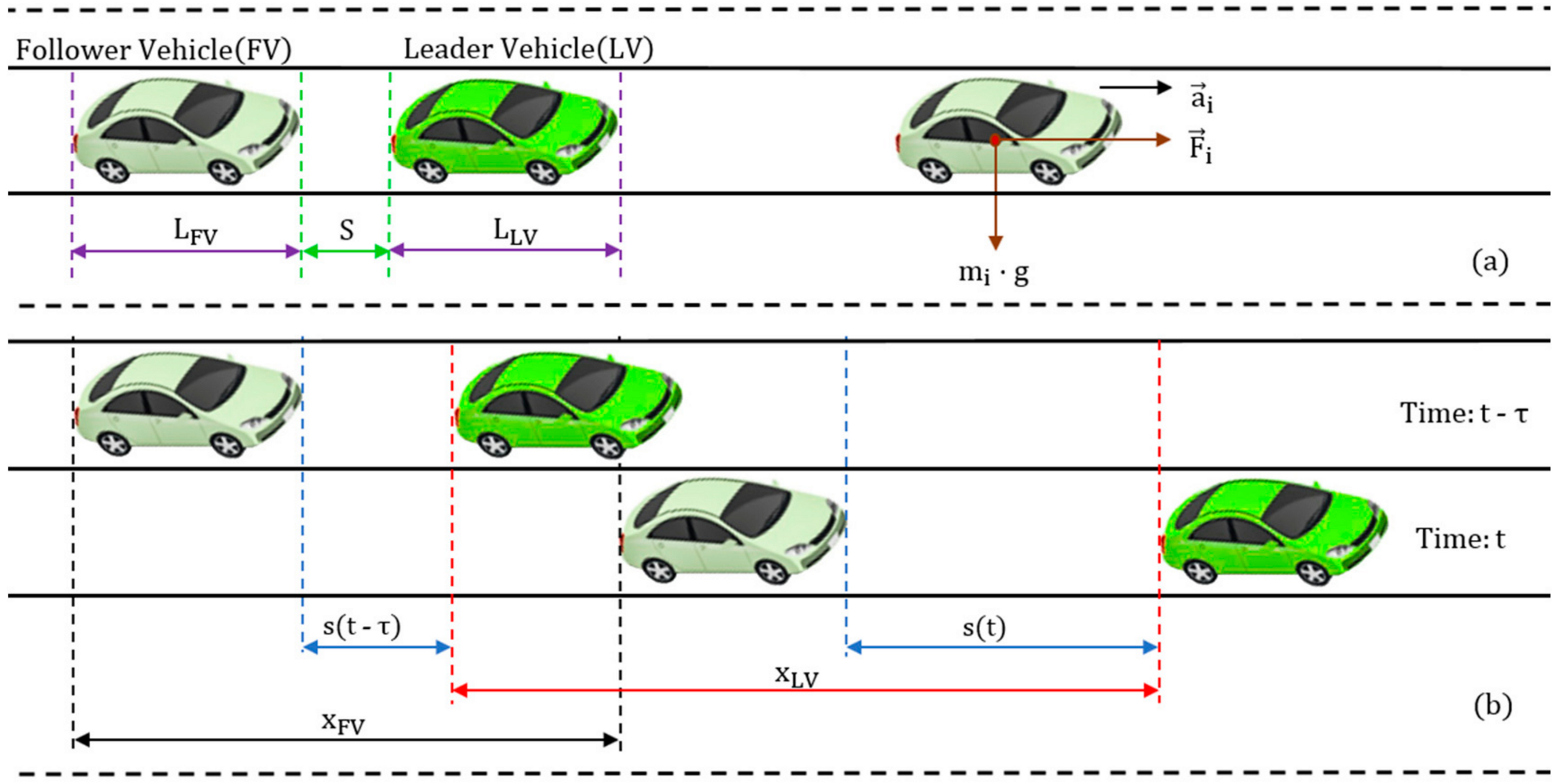
The car-following concept [
19] consists of the analysis of the interaction between two vehicles and their behavior on a road network. The vehicle ahead, called LV (leader vehicle), and the other vehicle, named FV (follower vehicle), are the main actors in this modeling approach. The FV “follows” the LV’s behavior and adapts its driving behavior accordingly, ensuring collision avoidance.
The main parameters of interest considered in this concept are vehicle position, velocity, acceleration/deceleration and the direction of movement.
In addition to the aforementioned parameters, other parameters that influence a vehicle’s movement behavior, some of which depend on the vehicle characteristics, are presented in
Figure 1a:
—length of FV;
—length of LV;
—standard safety interval distance between FV and LV;
—mass of the vehicle i where ;
-acceleration of gravity used to represent the weight of a vehicle according to mechanics theory (product between mass and acceleration of gravity);
—acceleration/deceleration value of the vehicle i where ;
—inertial force of the vehicle i where
that can be computed according to Relation (1), after applying Newton’s second law of motion:
To better understand the influence of the car-following model parameters,
Figure 1b illustrates the interaction of a LV and FV at time t
and
The parameters of interest for the vehicle’s movement behavior are:
—running distance of FV during a interval of time;
—running distance of LV during a interval of time;
—dynamic distance value between FV and LV at time t;
—dynamic distance value between FV and LV at time .
3.2. Car-Following Model
Based on previous assumptions and on MIMO (multiple input multiple output) systems theory, a state space representation of the car-following concept is needed.
A good way to expand the research possibilities for car-following models and create a framework for new optimal control approaches for these models is to follow the next three steps:
create a linear continuous system model without time-delay;
add the time-delay factor to the model;
create a discrete model to control the behavior of FV and LV.
According to the listed steps, the obtainment of car-following models, as proposed in [
38,
39], is further presented.
Using
and
as notations for car velocities,
and
for the running distances of the cars, and
and
for the car accelerations, the linear continuous car-following model can be described by system equations from Relation (2).
The standard safety distance S computation is done according to Relation (3) considering the vehicle average length
:
To transform the previous equations to the classic form for MIMO state space representation from Relation (4), it is necessary to define
,
(s—is the dynamic distance between two cars) and
:
where the vectors and matrixes are:
,
,
,
,
. In addition, we have
controllable and
observable; additionally the system eigenvalues are 0.
To introduce the time-delay
, we assume that
and
. Introducing these notations in Relation (4) yields the linear continuous time-delay car-following model as follows:
Considering that
, where T is the sampling period, Relation (6) is defined as:
If we rewrite Relation (5) according to Relation (6), we obtain the following relation:
If we consider
,
in the state equation and
in the output equation, we obtain the discrete car-following model, as in Relation (8).
3.3. Challenges in Car-Following Modeling
In car-following modeling, several situations when the FV and LV behavior can be influenced can appear. The most common is LV change. This situation usually occurs when a vehicle intends to start a lane change maneuver, or when a vehicle leaves the current road network using an exit point.
The challenges in these cases include the model of the deceleration process of neighboring vehicles, the acceleration of the vehicle that wants to change its current lane, respecting safe distances, the change of leader and follower roles and the switching of roles between FV and LV due to the LV’s low velocity. All these can be better explained by using the lane change concept.
4. Lane Change Behavior Estimation
A lane change can be defined as the decision taken by a driver to change his/her current lane. This action can be observed as a process that usually occurs in two main cases. The first case is when the LV has low velocity and the FV changes lane only for a while, before returning to its previous lane. In this case, the only reason for the change is the driver’s desire to move at a higher speed without changing his/her planned destination. The second case arises from issues like leaving the road network using an exit lane or possible future restrictions of lane changes that can influence the planned destination.
Based on previously explained situations, in a car-following model, the leader-change concept is a parameter. In all circumstances of lane changes, the LV is changed, even while switching roles between current LV and FV, or the introduction of a new LV from a new joined traffic lane.
4.1. Lane Change Process Modeling
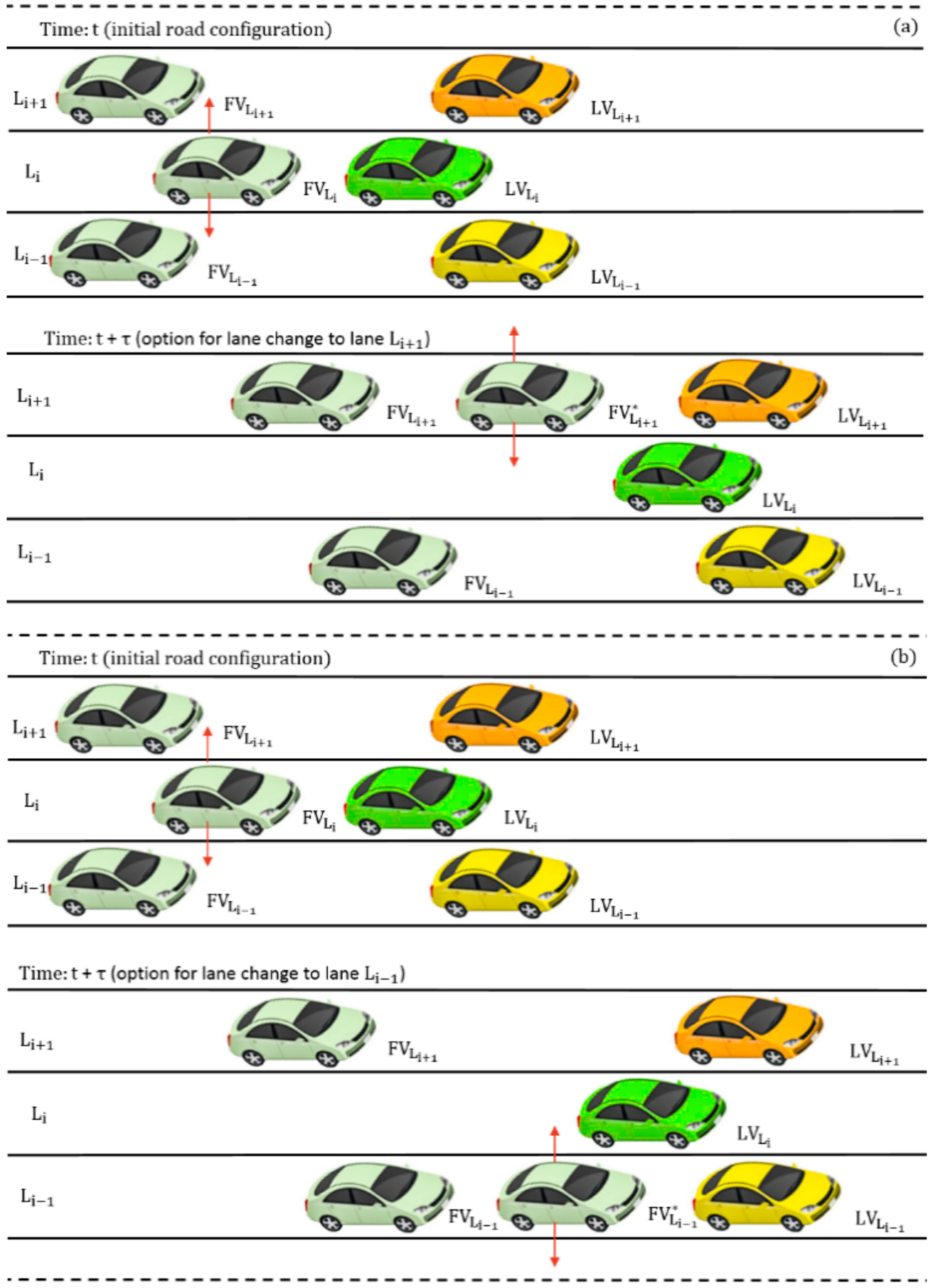
For a better understanding of lane change behavior,
Figure 2 shows all possible situations that can appear during this action for a road that has three lanes in the direction of movement. The relationships with the specific terms for car-following models are illustrated.
Figure 2 shows a possible lane change action during a road network crossing. We assume that we have one LV associated with each lane, and the position of the lanes are as follows:
—is the right lane,
—is the middle lane,
—the left lane. The purpose is to study the behavior of the FV from lane
. This car has two options to change its lane. If the choice is lane
, the
becomes the follower of the
(
Figure 2a). At this point, the driver can then choose to return to his/her previous lane or to leave the road network if lane
is a left exit lane. In the other case, by moving to lane
, the
becomes the follower of the
(
Figure 2b). Similar to the previous situation, the driver can further choose to return to his/her previous lane or leave the road network if lane
is a right exit. We can see that in all presented situations, the new role of a vehicle is highlighted with an asterisk, notation further used also in the case of parameters to identify the parameter value after a role change. In addition to the classic lane change based on a possible decision taken by the driver to modify his/her initial itinerary, a lane change action taken only based on the low velocity of the LV is also possible.
As shown before, the vehicle that initiates the lane change maneuver influences the behavior of the two vehicles from the current and the target lanes [
21]. To see that a lane change can lead to improvements in the individual local traffic situation of a driver, the incentive criterion was defined.
Consider the following notations for the accelerations of the vehicles involved in the
lane change action:
where
represents the acceleration of the
successor and assuming that we have symmetric lane changing rules, the incentive criterion is represented by Relation [
21]:
where
is the politeness factor that denotes the total advantage of the two immediately affected neighboring vehicles, and
is the switching threshold.
According to driving rules established by legislation, some lane changes are forbidden. Here, we can reformulate the incentive criterion based on asymmetric passing rules defined according to the majority of European countries’ traffic legislation [
21].
For asymmetric passing rules, two forms of incentive criterion can be defined:
lane change from left to right [
21]:
lane change from right to left [
21]:
where
are the accelerations adapted by the driver to the majority of European countries’ traffic legislation and
is a constant representing the keep-right directive of the lane change rule.
Another important criterion specific to this action is the safety criterion: the deceleration of the successor vehicle from target lane (
or
) shall not exceed a given acceleration safe limit, as defined by Equation (13) [
21].
Lane change behavior can be measured by calculating the lane changing rate using the relation below [
21]:
where
is the number of lane changes during a
interval of time on a section of road with a length of
kilometers.
4.2. Bayesian Reasoning for Lane Change Estimation
A lane change action can be considered a process where the estimations can be done while assuming a high level of uncertainty. This arises because of driver decisions that are hard to predict or plan. The driver acts based on real-time traffic conditions to maximize his/her chances to obtain a lower travel cost and reach a planned destination on time. In addition, the driver lane change action is also influenced by other drivers through the politeness factor, as presented before.
After admitting the existence of a level of uncertainty, we can say that this lane change action is a Bayesian specific problem. Here, the main conditions for a successful lane change are: to have a driver decision to initiate the action and the contribution of neighboring drivers to help this action happen. Other factors that have important roles are the routing alternatives associated with a lane at a vehicle entry point on the road network and the previously established destination.
Below, we briefly present the Bayes probabilistic concept and our proposal of this concept application based on the previously mentioned assumptions.
Bayes systems estimate the probability of an upcoming event occurrence based on posterior probabilities, which comprise prior, available information related to the conditions that can influence our system’s behavior. Briefly, Bayes’ theorem can be expressed as Equation (15) [
40,
41]:
In Bayes theory, the probability of event x is expressed conditioned on the observed event y, according to Relation (17). The prior probability distribution obtained for p(x) uses previous knowledge data. The influence of observed event
is represented by the conditional probability p(y|x), also known as the likelihood function. The form p(x|y) is called posterior probability, which can be used to establish the level of uncertainty in x after event y has been observed [
40,
41,
42].
The probability of event y conditioned by a known event x can be defined as (17) [
40,
42,
43].
Going further and considering x and y as independent events, the probability p(y,x) of event y conditioned by event x can be computed using Equation (18) [
40,
44].
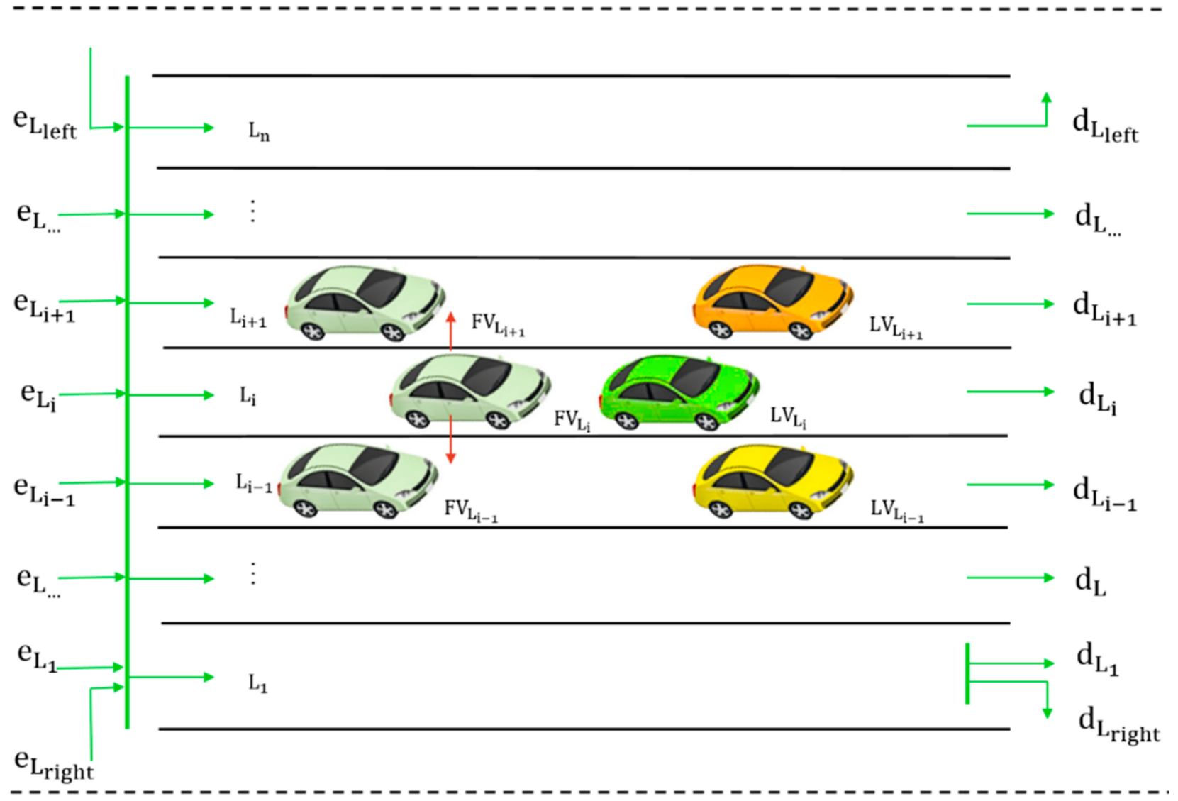
Our proposed approach is to compute the probabilistic estimator of a lane change action as an intersection of five Bayes probabilities, according to Equation (19) and
Figure 3. We can observe that lane
offers the possibility to go straight or leave the road network using a right exit, while lane
facilitates the driver’s decision to leave the road network using a left exit.
denotes the probability of the FV which joined the traffic link using the entrance lane
, and
the probability that FV will leave the link using the exit (destination) lane
. Probability
shows the level of influence of the LV’s velocity on the FV’s lane change decision from lane
. The significance of the other probabilities is related to the target lane probabilities associated with respect to FV and LV.
Based on previous assumptions, p was defined as the total advantage of the two immediately affected neighboring vehicles. In this case, the politeness factor
can be defined as a product of the last two conditional probabilities from Equation (19):
In this manner, Equation (19) becomes:
By expanding Equation (21) according to Bayes rule, we obtain:
After estimating the probability of a lane change action based on the probabilities from previous road networks crossings, it is necessary to introduce new notations, similar to the approach presented in [
40]. Lowercase notations will be used to represent the probabilities computed based on previous traffic data:
By replacing these notations in Equation (24), we can obtain the final form of estimated probability of a lane change action from lanes i to j:
Our approach also consists of modifications into lane changing rules. Furthermore, the relations that define these rules are as follows:
incentive criterion for symmetric lane changing rules:
incentive criterion for asymmetric lane changing rules—lane change from left to right:
incentive criterion for asymmetric lane changing rules—lane change from right to left:
5. Multiple Lane Road Car-Following Approach
5.1. Car-Following Model for Multiple Lane Road
Figure 4 shows a new car-following model extended to multiple-lane roads. This model, built based on the modeling theory presented in the third section, implements our proposal for estimating the probability of a lane change.
Considering the likelihood of initiating a lane change maneuver by driver c, the probabilities computed based on previous data and using Equation (24) offer the lane with the highest probability to be chosen by that driver from lane
. The driver decision c to perform a lane change maneuver is computed according to Equation (28), and its meaning can be summarized as the probability of not choosing lane
:
The acceleration and other parameters, like velocity and running distance for the target vehicle, are updated according to the specific rules of lane change actions. If there is not a driver decision for a lane change maneuver, the model behaves as a standard car-following model without incorporating the lane change rules into the vehicle behavior description.
For simplicity, we built a procedure for lane change behavior estimations considering incentive criteria for the symmetric lane changing rule. The simulation results are available in the Results section.
5.2. Fault Detection using Parity Equations
The residual computation starts from the discrete car-following model described by Equation (7), and follows the process described by [
12,
45]. A system works correctly only if the residuals are equal to zero, i.e., a nonzero residual may demonstrate a functional fault in the studied system [
12,
45]. The general relation that can define the computation for the q
th sampled output of the car-following model is:
In case of a time window of length
and shifted by
backwards, the equation becomes:
where vectors
and
are:
and the matrixes M and Q have the following values:
As the state vector
is unknown, the Relation (30) is multiplied by a vector
[
12]:
The residual
computation, that represents the parity signal, is described below, using the defined matrixes by Equations (31) and (32) as follows:
where
and
are permanently updated considering the incentive criteria defined by Equations (25)–(27) as the consequences of a possible lane change action according to Equations (28).
6. Experiment and Results
This section presents the results of the proposed multiple-lane car-following model in comparison with a separate, standard car-following model for each lane, as well as the fault detection results. Additionally, this section provides the implementation details and the input data used for the experiment. The purpose is to show that the proposed multiple-lane model is able to detect a lane-change maneuver and can change the model parameters accordingly. For this reason, each figure also shows the driver’s decision regarding a possible lane. The second part of this section presents the evolution of the residual values, which was based upon an analysis of the impact of possible faults on the system inputs.
6.1. Simulation Setup
6.1.1. Input Data
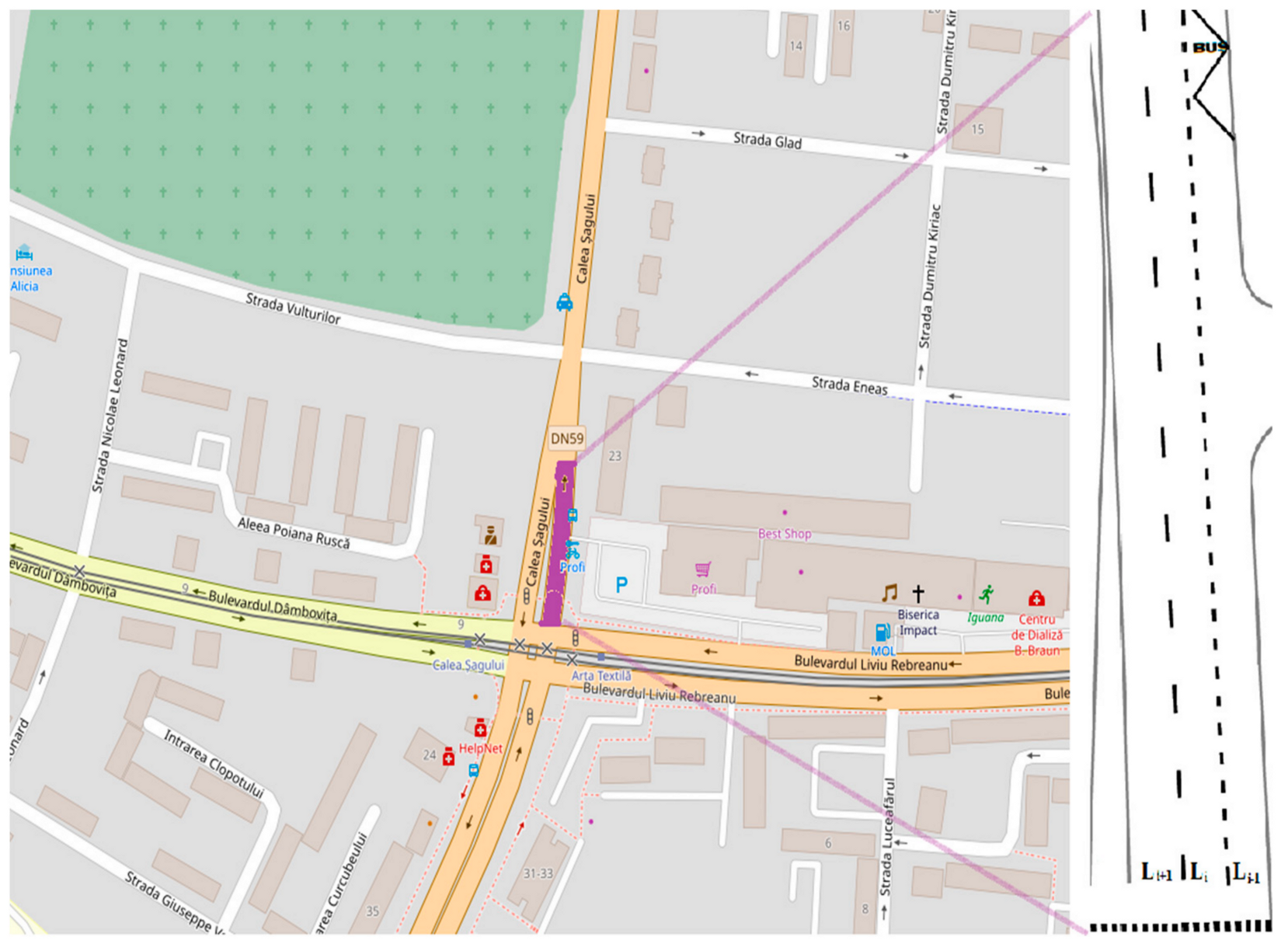
To show the practical application of the fault detection method based on parity equations, we present a case study for a three-lane road in Timisoara, Romania.
Figure 5 illustrates a real map of the studied section of road and its lane configuration.
The simulation used the data from
Table 1 as inputs. The table defines the velocities for the studied lanes and the probabilities of lane choice behavior. The number of vehicles considered in the probability and velocity computation consisted of raw data retrieved from inductive loops placed on the road network. The simulation applied a derivative for velocities to obtain the acceleration values as a first step, and further application led to the implementation of our proposal, as described in [
10].
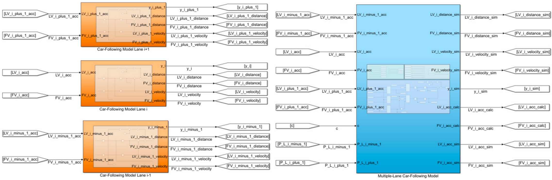
6.1.2. Simulation Model
To perform fault detection based on parity equations for the multiple-lane car-following model, a simulation was done in Simulink, part of MATLAB R2020a (MathWorks, Natick, MA, USA). Usually, the fault detection considers three types of models: nominal, observed, and the model with a defect. This paper assumed that the observed model had already incorporated faults as a result of the proposed computational approach. In this case, the implementation consisted of two main types of subsystems, as shown in
Figure 6: three separate blocks for the standard implementation of a car-following model, consisting of the nominal model (orange); and the proposed model for multiple-lane car-following, consisting of the observed model (blue).
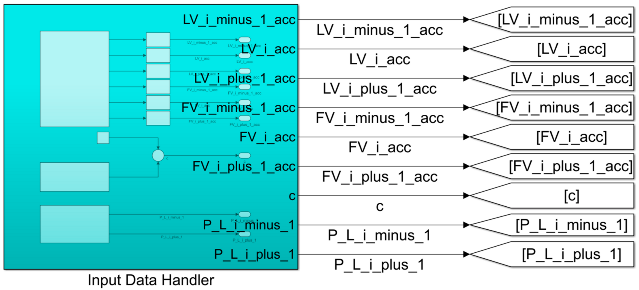
The transformation of velocity into acceleration is covered by the input handler subsystem, shown in
Figure 7. Here, a discrete-time derivative block was applied to the raw velocity data to transform them in acceleration data, ensuring the functionality of the previously presented blocks.
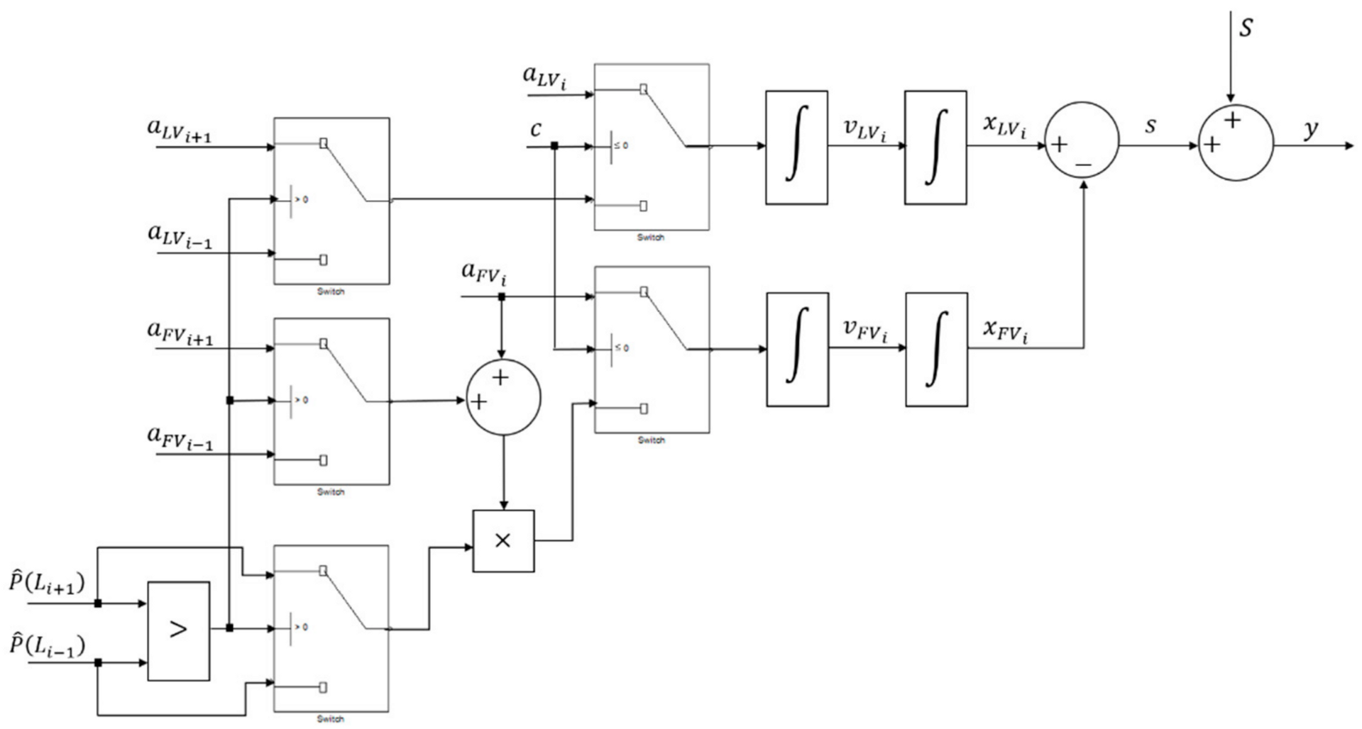
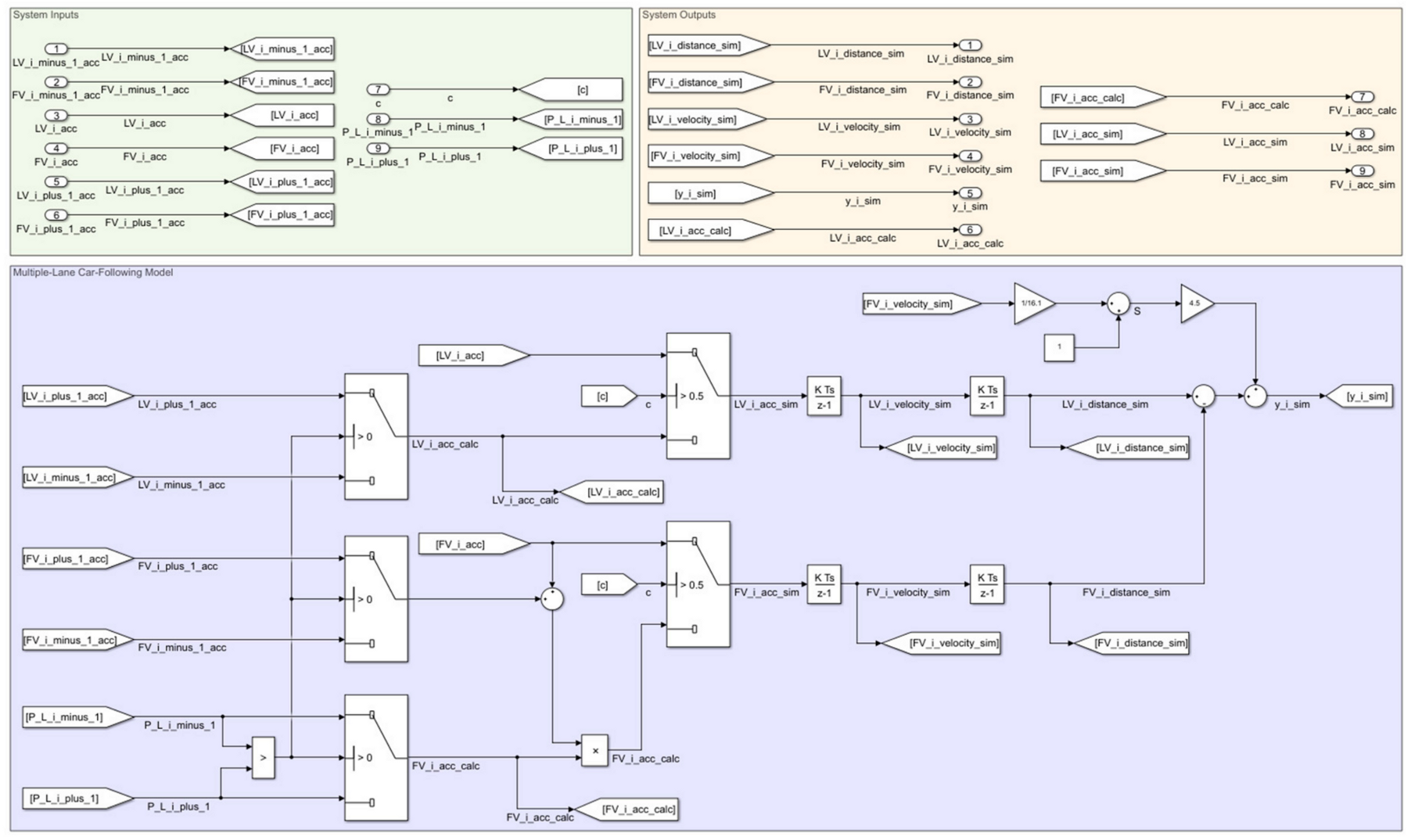
Figure 8 depicts the implementation of the model for monitoring possible lane change maneuvers from lane
to
or
The main outputs of this block are the LV and FV velocities and running distances, that are further used as input for the computation of the residuals. In the Simulink implementation, the residuals were the difference between the output of the standard car-following model block and the outputs from the proposed multiple-lane car-following model. It is necessary to mention that the standard safety distance S computation was done for both models according to Equation (2) [
39] and assuming that the vehicle average length
for passenger vehicles was
.
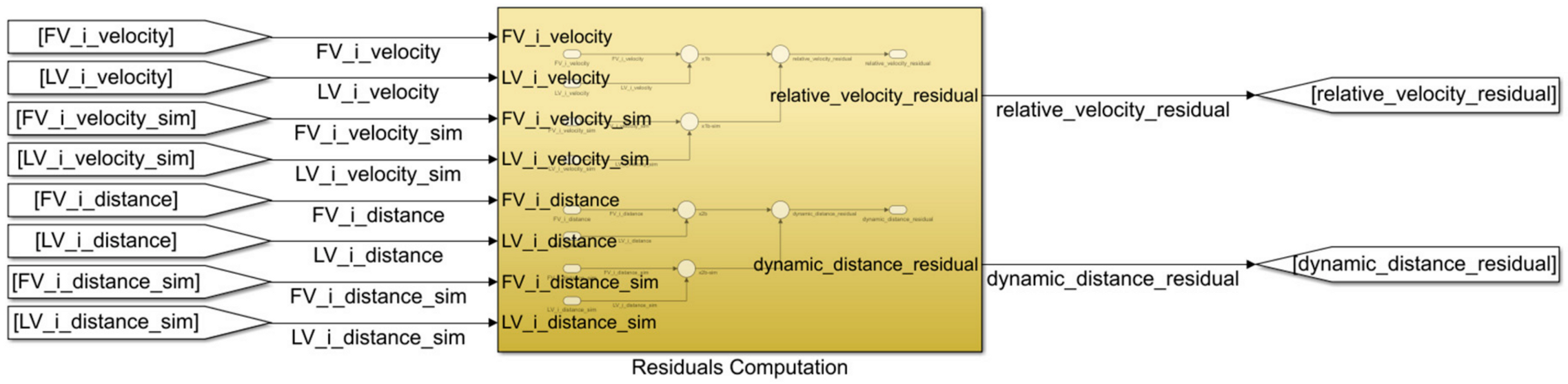
The subsystem shown in
Figure 9 covers the residual computation. The outputs are the
relative_velocity_residual and
dynamic_distance_residual, and consist of the differences between the values of
and
obtained from Equation (34) by using the nominal model and the observed model with faults introduced by the computation approach.
To simplify the obtained results,
Table A1 describes the mapping between the models defined in this paper and the signals used as simulations. Some of the internal states were passed as outputs from the subsystems for the creation of graphics. The table sets the parameter type based on the state-space representation concept.
6.2. Simulation Results
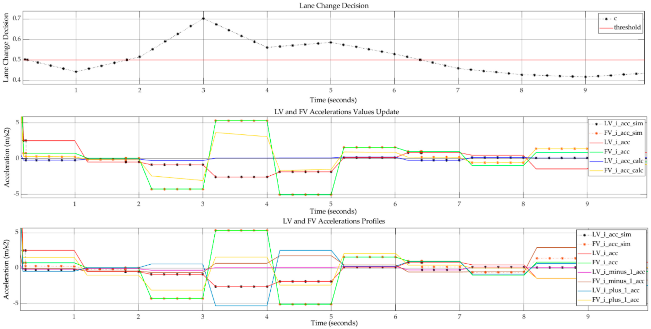
Figure 10 shows the acceleration profiles and the internal update of the acceleration values for LV and FV after c is greater or lower than the threshold. The threshold value was set to 0.50 and showed a greater than 50% chance of changing lanes. In this case, the simulated values for LV and FV were set to the calculated values, taking Equation (25) into account. For a better understanding of these switches of simulated acceleration values incorporating lane change actions, the case of a lane change action from
to
at time 0.2 s can be considered. The LV from lane
performs this action and starts to follow the movement behavior described by vehicles moving into lane
. The FV from lane L
i will also change its movement behavior due to the new LV after the initial LV changes lane. Another, similar case, but with a lane change from
to
, is observable at time 6.3 s.
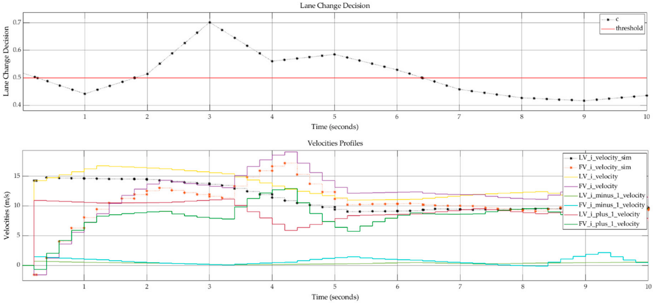
Changing acceleration values also implies a change of velocity.
Figure 11 shows an overview of the velocity values for all lanes, and incorporates a velocity change after a lane change maneuver. Here, the outputs from both the standard car-following model and the proposed approach can be seen.
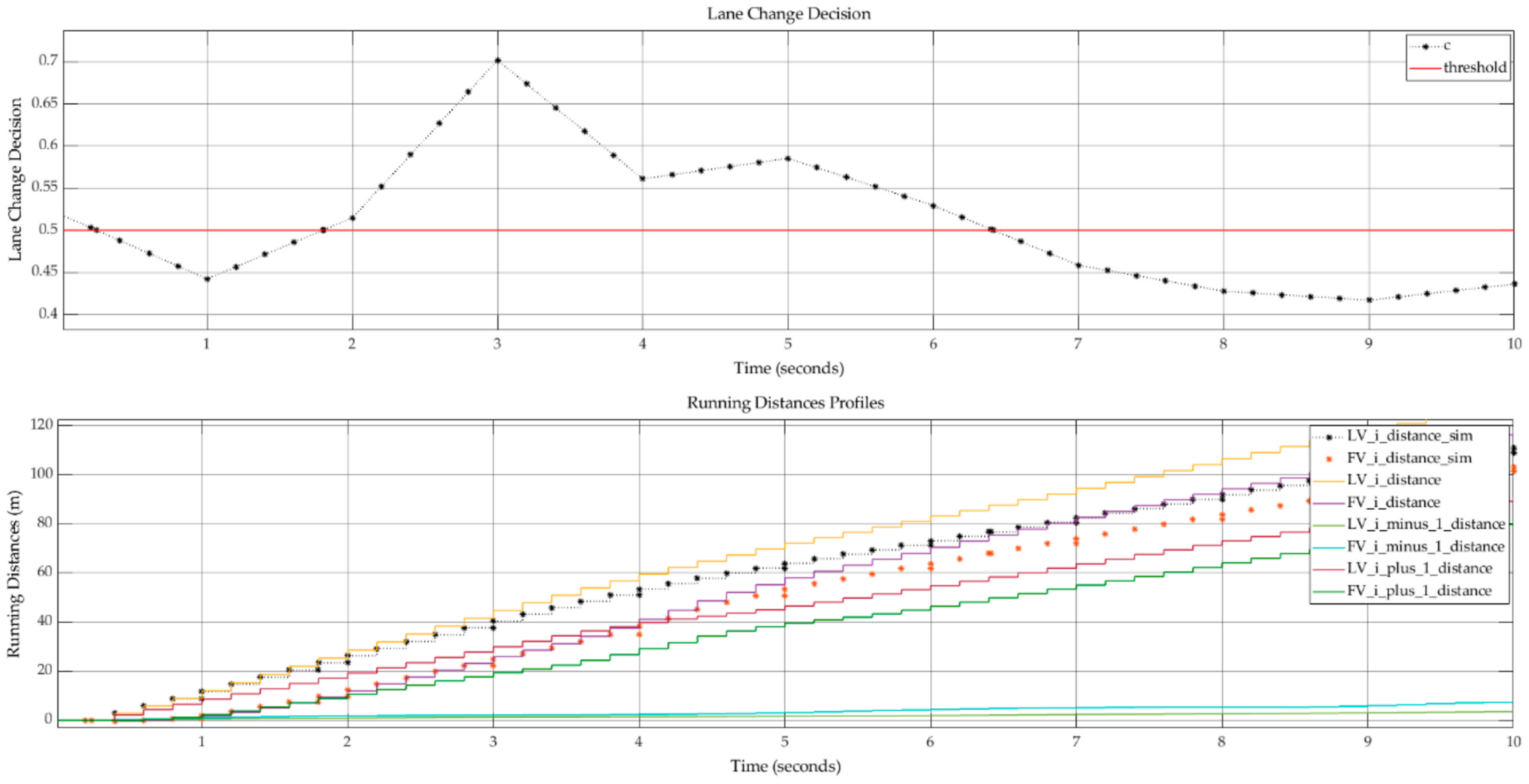
The running distances profiles shown in
Figure 12 create an overview of simulated distances by covering the lane change action and offering the evolution of the values after the action has taken place. The vehicles continue their movement based on different trajectories after a lane change action. Here, the disadvantage of the proposed approach can be seen, i.e., the incorporation of lane change behavior in the current lane does not highlight the impact on adjacent traffic lanes.
Here, a graphical comparison between the standard car-following model and the multiple-lane car-following model proposed in this paper is presented. The proposed model incorporated the lane change action and adapted the behavior of LV and FV from the new lane accordingly. The main disadvantage is that the current model cannot provide a view of the initial lane road traffic evolution in parallel.
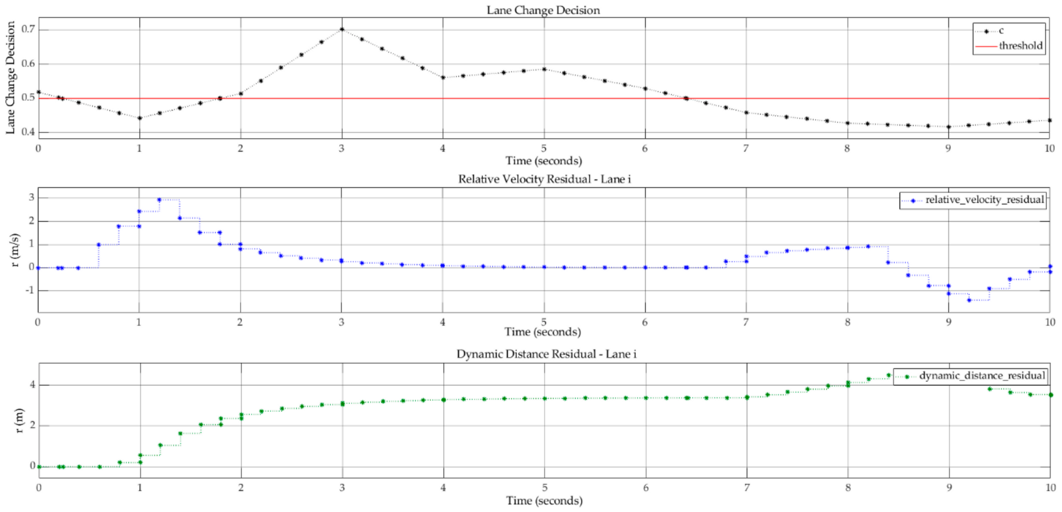
6.3. Fault Analysis
The fault analysis created an overview of the evolution of two residuals, i.e., relative velocity and dynamic distance, based on the movement in lane
.
Figure 13 depicts the influence of the lane change actions on the velocity and distance computation using the multiple-lane car-following model. The proposed model introduces faults when driver decision c has a low degree of uncertainty (i.e., c is near the 0.50 threshold with
). In other cases, when the driver decision is not affected by this low level of uncertainty, the relative velocity residual tends to zero. The dynamic distance residual has a continuous increasing trend based on the same pattern, and its value remains relatively constant in the absence of a low level of uncertainty.
7. Conclusions
This paper shows a multiple-lane car-following approach that allows the introduction of a new vehicle into a specific lane, and ensures the update of traffic parameters for an LV and a new FV. It should be noted that is a new car-following model that incorporates the behavior between the vehicles from the current and adjacent lanes. A fault detection analysis based on parity equations was performed for the proposed model.
The paper starts with a summary of current related works on microscopic traffic analysis, traffic parameters estimation methods, sensor networks applications and system fault detection.
Overviews of other car-following modeling approaches, lane change behavior estimation and fault detection using parity equations were mandatory for the creation of a new model that can adapt to multiple-lane roads.
The proposed model uses Bayesian probabilities as inputs to simulate driver decisions to initiating a lane change maneuver. The accelerations of LV and FV adapt according to these probabilities in the case of a lane change action taking place. This change of values also ensures compliance with the incentive criteria defined for lane changes.
Assuming that the proposed model introduces defects through the computational process, fault detection using parity equations is performed by adapting the general equations to our car-following model. The result of this fault detection consists of two residuals: that of relative velocity between LV and FV from the current lane, and that of the residual dynamic distance between LV and FV from the current lane without considering standard safety distance S.
The proposed model implementation using Simulink (MATLAB R2020a) proved the expected features. The simulation used data from a local traffic monitoring center as inputs and succeeded in showing the integration of a lane change action in a multiple-lane car-following model by modifying the rest of the traffic parameters accordingly. The paper presents, through the evolution of the residual values, an overview of the faults introduced by the proposed approach. The analysis showed that driver decision uncertainty represents the main source of faults.
The main drawback of the proposed approach is that it currently only shows the behavior of the LV and FV from a specific lane in relation with other lanes after the insertion of a new vehicle into the current lane. For this reason, the model is not suitable for a real-time switch from one lane to another to ensure lane change behavior monitoring for each lane. Future work will be focused on introducing an adaptive switch between road lanes to show the real-time updated traffic conditions for all lanes in parallel.
Author Contributions
Conceptualization, M.-D.P.; software, M.-D.P.; validation, O.P. and G.P.; writing—original draft preparation, M.-D.P.; writing—review and editing, O.P. and G.P.; supervision, O.P. and G.P. All authors have read and agreed to the published version of the manuscript.
Funding
This research received no external funding.
Acknowledgments
The data used for simulations were received from Timișoara City Hall—General Directorate of Roads, Bridges, Parking and Utility Networks—Traffic Monitoring Office, Timișoara, Romania (romanian official institution name: Primăria Municipiului Timișoara-Direcţia Generală Drumuri, Poduri, Parcaje și Rețele Utilitare–Birou Monitorizare Trafic, Timișoara, Romania) based on the approved request RE2019-002611/18.12.2019. The support is gratefully acknowledged.
Conflicts of Interest
The authors declare no conflict of interest.
Appendix A
Table A1.
Mapping between model parameters and simulation defined signals.
Table A1.
Mapping between model parameters and simulation defined signals.
| Parameter Type 1 | Model Parameter | Simulation Defined Signal | Significance |
|---|
| Inputs | for | LV_i_minus_1_acc | acceleration of LV from lane |
| for | LV_i_acc | acceleration of LV from lane |
| for | LV_i_plus_1_acc | acceleration of LV from lane |
| for | FV_i_minus_1_acc | acceleration of FV from lane |
| for | FV_i_acc | acceleration of FV from lane |
| for | FV_i_plus_1_acc | acceleration of FV from lane |
| c | c | driver decision to initiate a lane change maneuver |
| P_L_i_minus_1 | probability of lane change from to according to Equation (23) |
| P_L_i_plus_1 | probability of lane change from to according to Equation (23) |
| Internal calculated values for multiple-lane car-following model | for , | LV_i_acc_calc | calculated acceleration of new LV after lane change maneuver to , |
| for , | FV_i_acc_calc | calculated acceleration of new FV after lane change maneuver to , considering Equation (24) |
| S | S | standard safety distance calculated according to Equation (3) |
| Internal system states for standard car-following model | for | LV_i_minus_1_velocity | velocity of LV from lane |
| for | LV_i_velocity | velocity of LV from lane |
| for | LV_i_plus_1_velocity | velocity of LV from lane |
| for | FV_i_minus_1_velocity | velocity of FV from lane |
| FV_i_velocity | velocity of FV from lane |
| for | FV_i_plus_1_velocity | velocity of FV from lane |
| for | LV_i_minus_1_distance | running distance of LV from lane |
| for | LV_i_distance | running distance of LV from lane |
| for | LV_i_plus_1_distance | running distance of LV from lane |
| for | FV_i_minus_1_distance | running distance of FV from lane |
| FV_i_distance | running distance of FV from lane |
| for | FV_i_plus_1_distance | running distance of FV from lane |
| Outputs for standard car-following model | for | y_i_minus_1 | dynamic distance between LV and FV from considering S |
| for | y_i | dynamic distance between LV and FV from considering S |
| for | y_i_plus_1 | dynamic distance between LV and FV from considering S |
| Internal system states for multiple-lane car-following model | simulated for | LV_i_acc_sim | simulated acceleration of LV (considers a possible lane change maneuver) |
| simulated for | FV_i_acc_sim | simulated acceleration of FV (considers a possible lane change maneuver) |
| simulated for | LV_i_velocity_sim | simulated velocity of LV (considers a possible lane change maneuver) |
| simulated for | FV_i_velocity_sim | simulated velocity of FV (considers a possible lane change maneuver) |
| simulated for | LV_i_distance_sim | simulated running distance of LV (considers a possible lane change maneuver) |
| simulated for | FV_i_distance_sim | simulated running distance of FV (considers a possible lane change maneuver) |
| Output for multiple-lane car-following model | simulated y for | y_i_sim | simulated dynamic distance between LV and FV from considering S |
| Output from residuals computation subsystem | r for from | relative_velocity_residual | residual of relative velocity between LV and FV from |
| r for from | dynamic_distance_residual | residual of dynamic distance between LV and FV from without considering S |
References
- Cunha, J.; Batista, N.; Cardeira, C.; Melicio, R. Wireless Networks for Traffic Light Control on Urban and Aerotropolis Roads. J. Sens. Actuator Netw. 2020, 9, 26. [Google Scholar] [CrossRef]
- Hammoudeh, M.; Arioua, M. Sensors and Actuators in Smart Cities. J. Sens. Actuator Netw. 2018, 7, 8. [Google Scholar] [CrossRef] [Green Version]
- Riouali, Y.; Benhlima, L.; Bah, S. Toward a Global WSN-Based System to Manage Road Traffic. In Proceedings of the International Conference on Future Networks and Distributed Systems—ICFNDS ’17, Cambridge, UK, 19–20 July 2017; ACM Press: Cambridge, UK, 2017; pp. 1–6. [Google Scholar]
- Raza, N.; Jabbar, S.; Han, J.; Han, K. Social vehicle-to-everything (V2X) communication model for intelligent transportation systems based on 5G scenario. In Proceedings of the 2nd International Conference on Future Networks and Distributed Systems—ICFNDS ’18, Amman, Jordan, 26–27 June 2018; ACM Press: Amman, Jordan, 2018; pp. 1–8. [Google Scholar]
- Ateya, A.; Muthanna, A.; Gudkova, I.; Abuarqoub, A.; Vybornova, A.; Koucheryavy, A. Development of Intelligent Core Network for Tactile Internet and Future Smart Systems. J. Sens. Actuator Netw. 2018, 7, 1. [Google Scholar] [CrossRef] [Green Version]
- Arena, F.; Pau, G.; Severino, A. A Review on IEEE 802.11p for Intelligent Transportation Systems. J. Sens. Actuator Netw. 2020, 9, 22. [Google Scholar] [CrossRef]
- Yu, B.; Wu, M.; Wang, S.; Zhou, W. Traffic Simulation Analysis on Running Speed in a Connected Vehicles Environment. Int. J. Environ. Res. Public Health 2019, 16, 4373. [Google Scholar] [CrossRef] [PubMed] [Green Version]
- Al-Ahmadi, H.M.; Jamal, A.; Reza, I.; Assi, K.J.; Ahmed, S.A. Using Microscopic Simulation-Based Analysis to Model Driving Behavior: A Case Study of Khobar-Dammam in Saudi Arabia. Sustainability 2019, 11, 3018. [Google Scholar] [CrossRef] [Green Version]
- Lopez, P.A.; Behrisch, M.; Bieker-Walz, L.; Erdmann, J.; Flotterod, Y.-P.; Hilbrich, R.; Lucken, L.; Rummel, J.; Wagner, P.; WieBner, E. Microscopic Traffic Simulation using SUMO. In Proceedings of the 2018 21st International Conference on Intelligent Transportation Systems (ITSC), Maui, HI, USA, 4–7 November 2018; IEEE: Maui, HI, USA, 2018; pp. 2575–2582. [Google Scholar]
- Pop, M.-D.; Proştean, O.; Proştean, G. Multiple Lane Road Car-Following Model using Bayesian Reasoning for Lane Change Behavior Estimation: A Smart Approach for Smart Mobility. In Proceedings of the 3rd International Conference on Future Networks and Distributed Systems—ICFNDS ’19, Paris, France, 1–2 July 2019; ACM Press: Paris, France, 2019; pp. 1–8. [Google Scholar]
- Isermann, R. Supervision, fault-detection and diagnosis methods—A short introduction. In Fault-Diagnosis Applications; Springer: Berlin/Heidelberg, Germany, 2011; pp. 11–45. ISBN 9783642127663. [Google Scholar]
- Isermann, R. Fault detection with parity equations. In Fault-Diagnosis Systems; Springer: Berlin/Heidelberg, Germany, 2006; pp. 197–229. ISBN 9783540241126. [Google Scholar]
- Tao, L.; Lei, J. A car following model with the backward looking effect and next-nearest-neighbor interaction in relative velocity. In Proceedings of the 2009 International Conference on Test and Measurement, Hong Kong, China, 5 December 2009; Volume 2, pp. 429–432. [Google Scholar]
- Aycin, M.F.; Benekohal, R.F. Linear Acceleration Car-Following Model Development and Validation. Transp. Res. Rec. 1998, 1644, 10–19. [Google Scholar] [CrossRef]
- Tang, L.; Yang, X.; Kan, Z.; Li, Q. Lane-Level Road Information Mining from Vehicle GPS Trajectories Based on Naïve Bayesian Classification. ISPRS Int. J. Geo-Inf. 2015, 4, 2660–2680. [Google Scholar] [CrossRef] [Green Version]
- Ossen, S.; Hoogendoorn, S.P.; Gorte, B.G.H. Interdriver Differences in Car-Following: A Vehicle Trajectory–Based Study. Transp. Res. Rec. 2006, 1965, 121–129. [Google Scholar] [CrossRef]
- Meng, F.; Zhang, W.; Wang, J. Driver’s car-following and lane-changing models: An experimental study. In Proceedings of the 2011 IEEE 18th International Conference on Industrial Engineering and Engineering Management, Changchun, China, 3–5 September 2011; Part 3. pp. 2045–2048. [Google Scholar]
- Zaky, A.B.; Gomaa, W.; Khamis, M.A. Car Following Markov Regime Classification and Calibration. In Proceedings of the 2015 IEEE 14th International Conference on Machine Learning and Applications (ICMLA), Miami, FL, USA, 9–11 December 2015; pp. 1013–1018. [Google Scholar]
- Rothery, R.W. Car following models. In Traffic Flow Theory: A State-of-the-Art; Gartner, N., Messer, C.J., Rathi, A.K., Eds.; Committee on Traffic Flow Theory and Characteristics (AHB45), Turner-Fairbank Highway Research Center: McLean, VA, USA, 2001; pp. 4-1–4-42. [Google Scholar]
- Farooq, D.; Juhasz, J. Simulation-Based Analysis of the Effect of Significant Traffic Parameters on Lane Changing for Driving Logic “Cautious” on a Freeway. Sustainability 2019, 11, 5976. [Google Scholar] [CrossRef] [Green Version]
- Kesting, A.; Treiber, M.; Helbing, D. General Lane-Changing Model MOBIL for Car-Following Models. Transp. Res. Rec. 2007, 1999, 86–94. [Google Scholar] [CrossRef] [Green Version]
- Yang, D.; Zhu, L.; Yang, F.; Pu, Y. Modeling and Analysis of Lateral Driver Behavior in Lane-Changing Execution. Transp. Res. Rec. 2015, 2490, 127–137. [Google Scholar] [CrossRef]
- Gao, K.; Yan, D.; Yang, F.; Xie, J.; Liu, L.; Du, R.; Xiong, N. Conditional Artificial Potential Field-Based Autonomous Vehicle Safety Control with Interference of Lane Changing in Mixed Traffic Scenario. Sensors 2019, 19, 4199. [Google Scholar] [CrossRef] [PubMed] [Green Version]
- Chen, D.; Ahn, S.; Bang, S.; Noyce, D. Car-Following and Lane-Changing Behavior Involving Heavy Vehicles. Transp. Res. Rec. 2016, 2561, 89–97. [Google Scholar] [CrossRef]
- Tianyu Zhang; Qian Zhao; Kilho Shin; Yukikazu Nakamoto Bayesian-Optimization-Based Peak Searching Algorithm for Clustering in Wireless Sensor Networks. J. Sens. Actuator Netw. 2018, 7, 2.
- Casillo, M.; Coppola, S.; De Santo, M.; Pascale, F.; Santonicola, E. Embedded Intrusion Detection System for Detecting Attacks over CAN-BUS. In Proceedings of the 2019 4th International Conference on System Reliability and Safety (ICSRS), Rome, Italy, 20–22 November 2019; IEEE: Rome, Italy, 2019; pp. 136–141. [Google Scholar]
- Merenda, M.; Praticò, F.G.; Fedele, R.; Carotenuto, R.; Della Corte, F.G. A Real-Time Decision Platform for the Management of Structures and Infrastructures. Electronics 2019, 8, 1180. [Google Scholar]
- Deckert, J.; Desai, M.; Deyst, J.; Willsky, A. F-8 DFBW sensor failure identification using analytic redundancy. IEEE Trans. Autom. Contr. 1977, 22, 795–803. [Google Scholar] [CrossRef]
- Lu, X.-Y.; Varaiya, P.; Horowitz, R.; Palen, J. Faulty Loop Data Analysis/Correction and Loop Fault Detection. In Proceedings of the 15th ITS World Congress, New York, NY, USA, 16–20 November 2008; pp. 1–12. [Google Scholar]
- Coifman, B.; Dhoorjaty, S. Event Data-Based Traffic Detector Validation Tests. J. Transp. Eng. 2004, 130, 313–321. [Google Scholar] [CrossRef] [Green Version]
- Widhalm, P.; Koller, H.; Ponweiser, W. Identifying faulty traffic detectors with Floating Car Data. In Proceedings of the 2011 IEEE Forum on Integrated and Sustainable Transportation Systems, Vienna, Austria, 29 June–1 July 2011; pp. 103–108. [Google Scholar]
- Kurian, N.A.; Thomas, A.; George, B. Automated fault diagnosis in Multiple Inductive Loop Detectors. In Proceedings of the 2014 Annual IEEE India Conference (INDICON), Pune, India, 11–13 December 2014; IEEE: Pune, India, 2014; pp. 1–5. [Google Scholar]
- Pouliezos, A.D.; Stavrakakis, G.S. Analytical Redundancy Methods. In Real Time Fault Monitoring of Industrial Processes; Springer Netherlands: Dordrecht, The Netherlands, 1994; pp. 93–178. ISBN 9789048143740. [Google Scholar]
- Gertler, J. Diagnosing parametric faults: From parameter estimation to parity relations. In Proceedings of the 1995 American Control Conference—ACC’95, Seattle, WA, USA, 21–23 June 1995; American Autom Control Council: Seattle, WA, USA, 1995; Volume 3, pp. 1615–1620. [Google Scholar]
- Gertler, J. Fault detection and isolation using parity relations. Control Eng. Pract. 1997, 5, 653–661. [Google Scholar] [CrossRef]
- Wurtenberger, M.; Hofling, T. Vehicle supervision by bilinear parity equations. In Proceedings of the 1995 American Control Conference—ACC’95, Seattle, WA, USA, 21–23 June 1995; American Autom Control Council: Seattle, WA, USA, 1995; Volume 3, pp. 1662–1666. [Google Scholar]
- Yin, B.; Dridi, M.; El Moudni, A. Adaptive Traffic Signal Control for Multi-intersection Based on Microscopic Model. In Proceedings of the 2015 IEEE 27th International Conference on Tools with Artificial Intelligence (ICTAI), Vietri sul Mare, Italy, 9–11 November 2015; pp. 49–55. [Google Scholar]
- Pan, D.; Zheng, Y. Optimal control and discrete time-delay model of car following. In Proceedings of the 2008 7th World Congress on Intelligent Control and Automation, Chongqing, China, 25–27 June 2008; pp. 5657–5661. [Google Scholar]
- Khodayari, A.; Kazemi, R.; Ghaffari, A.; Manavizadeh, N. Modeling and intelligent control design of car following behavior in real traffic flow. In Proceedings of the 2010 IEEE Conference on Cybernetics and Intelligent Systems, Singapore, 28–30 June 2010; pp. 261–266. [Google Scholar]
- Pop, M.-D.; Prostean, O. Bayesian Reasoning for OD Volumes Estimation in Absorbing Markov Traffic Process Modeling. In Proceedings of the 2019 4th MEC International Conference on Big Data and Smart City (ICBDSC), Muscat, Oman, 15–16 January 2019; IEEE: Muscat, Oman, 2019; pp. 1–6. [Google Scholar]
- Bishop, C.M. Pattern recognition and machine learning. In Information Science and Statistics; Springer: New York, NY, USA, 2006; pp. 21–24. ISBN 9780387310732. [Google Scholar]
- Barber, D. Bayesian Reasoning and Machine Learning; Cambridge University Press: Cambridge, UK; New York, NY, USA, 2012; pp. 7–11. ISBN 9780521518147. [Google Scholar]
- Pamuła, T.; Król, A. The Traffic Flow Prediction Using Bayesian and Neural Networks. In Intelligent Transportation Systems—Problems and Perspectives; Sładkowski, A., Pamuła, W., Eds.; Springer International Publishing: Cham, Switzerland, 2016; Volume 32, pp. 105–126. ISBN 9783319191492. [Google Scholar]
- Akamatsu, T. Cyclic flows, Markov process and stochastic traffic assignment. Transp. Res. Part B Methodol. 1996, 30, 369–386. [Google Scholar] [CrossRef] [Green Version]
- Kratz, F.; Nuninger, W.; Ploix, S. Fault detection for time-delay systems: A parity space approach. In Proceedings of the 1998 American Control Conference. ACC (IEEE Cat. No.98CH36207), Philadelphia, PA, USA, 26 June 1998; IEEE: Philadelphia, PA, USA, 1998; Volume 4, pp. 2009–2011. [Google Scholar]
| Publisher’s Note: MDPI stays neutral with regard to jurisdictional claims in published maps and institutional affiliations. |
© 2020 by the authors. Licensee MDPI, Basel, Switzerland. This article is an open access article distributed under the terms and conditions of the Creative Commons Attribution (CC BY) license (http://creativecommons.org/licenses/by/4.0/).


