
Green Bonds for the Transition to a Low-Carbon Economy


1
Economics Department, The New School, 66 West 12th Street, New York, NY 10011, USA
2
Faculty of Economics and Business Administration, University of Bielefeld, Universitätsstraße 25, 33615 Bielefeld, Germany
3
International Institute for Applied Systems Analysis (IIASA), Schloßplatz 1, 2361 Laxenburg, Austria
*
Author to whom correspondence should be addressed.
Econometrics 2022, 10(1), 11; https://0-doi-org.brum.beds.ac.uk/10.3390/econometrics10010011
Submission received: 31 October 2021
/
Revised: 19 February 2022
/
Accepted: 21 February 2022
/
Published: 2 March 2022
(This article belongs to the Collection Econometric Analysis of Climate Change)
Abstract
:The green bond market is emerging as an impactful financing mechanism in climate change mitigation efforts. The effectiveness of the financial market for this transition to a low-carbon economy depends on attracting investors and removing financial market roadblocks. This paper investigates the differential bond performance of green vs non-green bonds with (1) a dynamic portfolio model that integrates negative as well as positive externality effects and via (2) econometric analyses of aggregate green bond and corporate energy time-series indices; as well as a cross-sectional set of individual bonds issued between 1 January 2017, and 1 October 2020. The asset pricing model demonstrates that, in the long-run, the positive externalities of green bonds benefit the economy through positive social returns. We use a deterministic and a stochastic version of the dynamic portfolio approach to obtain model-driven results and evaluate those through our empirical evidence using harmonic estimations. The econometric analysis of this study focuses on volatility and the risk–return performance (Sharpe ratio) of green and non-green bonds, and extends recent econometric studies that focused on yield differentials of green and non-green bonds. A modified Sharpe ratio analysis, cross-sectional methods, harmonic estimations, bond pairing estimations, as well as regression tree methodology, indicate that green bonds tend to show lower volatility and deliver superior Sharpe ratios (while the evidence for green premia is mixed). As a result, green bond investment can protect investors and portfolios from oil price and business cycle fluctuations, and stabilize portfolio returns and volatility. Policymakers are encouraged to make use of the financial benefits of green instruments and increase the financial flows towards sustainable economic activities to accelerate a low-carbon transition.
JEL Classification:
C610; G120; O380; Q5801. Introduction
Sustainable economic growth entails changes in production, consumption and, therefore, also in the form of financing “green investment”. Since financial markets can appear as a roadblock1 or a bridge in the transition to a low-carbon economy, it is important to understand investment decisions and financial performance regarding green assets as compared to conventional assets. The connection between externality theory from macroeconomics (growth theory) and empirical studies in green finance—asset pricing, bond yields, and the dynamic portfolio approach—is central. The portfolio decisions with respect to green and non-green (brown, i.e., fossil fuel-based, or conventional, i.e., plain vanilla) bonds are studied in the context of a dynamic portfolio model. In a finance role, the possibility that a gradual replacement of fossil fuel investments with green investments can reduce negative externalities, create positive externalities, and improve wealth accumulation is explored. The theoretical part includes a generic model of asset pricing and dynamic portfolio decisions concerning the shift from brown to green investments by including positive and negative economic externalities. In the empirical part, we focus on the performance of bond-financed green investments to analyze the differential bond performance of green and non-green bonds.
Microeconomic theory and models have long recognized that market decisions and market mechanisms have positive or negative external effects. However, macroeconomic models with externalities became more widely used in endogenous growth theory. Economic investments can have positive feedback effects impacting output through scale effects, for example, through some increasing returns to scale or Romer types of inventive investments; see Greiner et al. (2005). Negative externality effects have also been studied in macroeconomic growth theory (see Barro and Sala-i-Martin 2004).
However, what has not been studied sufficiently are the positive and negative feedback effects, arising on the real side of the economy, impacting the asset pricing, financial returns, and portfolio decisions of investors. There is now recent work on exploring how negative externalities arising from GHG emissions, and the subsequent damage and disaster risks, impact asset value and returns. Engle et al. (2020) study the impact of climate disaster news on asset risks and portfolio decisions concerning equity portfolios of green and fossil fuel-based equity in an extended Markowitz portfolio model. There are also studies on the green and conventional (and fossil fuel-based) bonds and how those asset returns and volatility are impacted by disaster or fuel price shocks.2
In the current paper, we first present a dynamic asset price model studying a generic link between the real economy with externalities, asset pricing, and dynamic portfolio decisions, resembling the work of Merton (1973) on dynamic portfolio decisions (See also Chiarella et al. 2016). We then, more specifically, introduce green and fossil fuel-based bonds into the dynamic portfolio framework, using some stylized movements of returns obtained from fast Fourier transform (FFT) and harmonic estimations of actual data from the US economy (As in Chiarella et al. 2016 and Semmler and Hsiao 2011). Once the positive and negative externalities are introduced, the asset price and portfolio allocation effects are studied and the fate of the evolution of wealth is explored. This work contributes to the existing literature by providing a dynamic portfolio model adjusted to account for climate externalities, and by relying on both endogenous growth theory and real data from the financial market performance of green and fossil fuel bonds. With the use of a suitable dynamic portfolio model, we offer a theoretical background for the econometric part, to provide a clearer view of what one would empirically expect. Its innovation is to use a dynamic (rather than static) portfolio to assess the yield differential and wealth accumulation between green and conventional bonds. An outlook for a stochastic version of this model is also presented in the Appendix B to account for financial market risks in the portfolio decision model.
The empirical section contributes to the econometric analysis literature of green finance by bringing together new empirical analysis tools for financial data, with a cross-sectional analysis approach to studying the drivers for green and conventional bonds’ performance. Recently developed financial diversification measures are used to analyze aggregate time series indices and apply multi-variate regressions, regression tree models, and a pairing algorithm for studying the differential performance of green and conventional bonds. Subsets of the energy sector, such as green renewable energy and fossil fuel bonds, are also explored. While the main focus is the reward-to-risk ratio (Sharpe ratio measure) for the bond performance analysis and various volatility measures (over ranges of 30 days, 90 days, and 260 days) we also provide evidence for primary and secondary market returns (using yield at issue and yield to maturity, respectively) in the Appendix C.
2. Theoretical and Empirical Literature
2.1. Theoretical Literature
The study of a portfolio dynamics with green and fossil fuel assets is undertaken based on a dynamic portfolio model, such as the one in Merton (1973), but improved on to account for climate externalities and different performance of climate-related assets. Merton (1973) proposes a dynamic model for investment decisions in which preferences are given by the utility of consumption, allowing for a different portfolio set depending on the decision horizon. When long-term climate risks hold, an intertemporal dynamic model can provide a better picture of portfolio decisions than static mean-variance models, such as the Capital Asset Pricing Model (CAPM). Conventional portfolio models are mostly influenced by the Markowitz mean-variance approach (Markowitz 1952) and Tobins’ mutual fund theorem (Tobin 1958).
The CAPM is a static model in which investors define, for a given wealth, their portfolios by balancing expected financial returns and risks, choosing between risky and risk-free assets. However, this model has an important drawback (Sharpe 1964; Lintner 1965).
This type of model does not capture the intertemporal dynamic of investor preferences and market changes over time, creating limitations to evaluate the climate impact on portfolio allocation. CAPM models do not consider that decisions are made under constraints, returns are not fixed over time, investors have different preferences for different risky assets, and time horizons are not the same for every investor (See Semmler 2011 and Chiarella et al. 2016). Moreover, conventional portfolio models with mean reversion returns are widely used (See Campbell and Viceira 2002 and Munk 2012). However, climate dynamics depend on intergenerational conflicts between current and future generations, are influenced by the share of green and fossil-fuel activities, and are formed by nonlinear dynamics. More recently, Campbell and Viceira (2002), Semmler (2011), and Chiarella et al. (2016) advance the original Merton model and provide a better framework to deal with nonlinearities, but still do not consider the externalities associated with green and fossil fuel assets.
Recently, contributions to Merton’s portfolio models adapt investors’ decisions to climate constraints. Engle et al. (2020) propose a dynamic portfolio model in which investors build mimic portfolios able to hedge against climate risks over the whole holding period, based on the short-term impact of news related to physical and transition risks. Semmler et al. (2020) provide an adjusted dynamic portfolio decision model, accounting for green innovation expenses in the utility function as well as for externality effects. As in endogenous growth macro models from Romer’s tradition, such as Romer (1986) and Greiner et al. (2005) and Acemoglu et al. (2012), human capital drives technical change and impacts long-run outcomes.
In this model, neglecting to invest in green technologies can lower returns for the portfolio in the long run due to negative externality effects and realized risks resulting from CO2 emissions (for example, disrupted production processes due to environmental damages). Negative externalities will harm returns and the accumulation of wealth will be lower. This is often the case, as argued by Davies et al. (2014), due to short-termism by cash flow-oriented investors. An improved version of this dynamic portfolio model with climate externalities is presented in Section 3. We introduce green and fossil fuel-based bonds into the dynamic portfolio framework, using some stylized movements of returns obtained from FFT, as in Chiarella et al. (2016) and Semmler and Hsiao (2011), of actual data from the US economy, adjusted to account for climate policy and externalities.3
By integrating positive and negative externalities from growth theory into dynamic asset-price and portfolio theory, higher returns on green bonds are expected, since some positive long-run externalities are to be expected. In contrast, one would expect lower returns in the long run for conventional (or fossil fuel-based) bonds, since, following the Pigouvian argument that the negative externalities have to be paid in some way, a lower return would be expected.
As to positive externality effects, in terms of a macro model—for the portfolio framework—we consider an endogenous growth-type macro model with externalities, as a Romer type of growth model with expenditure for innovations impacting economic growth rates (see Greiner et al. 2005).
In terms of modeling (See Semmler et al. 2020) the possibility of having a fraction of accumulated wealth going into consumption and an additional fraction spent on resources for new technologies can be included. As in Romer (1986), we assume this latter fraction as being spent on human capital-creating innovations. Yet, within the resource allocation for innovations, either for green or fossil fuel-based innovations, the latter is assumed to generate negative externalities in the long run. Thus, this spending is again subdivided into two purposes, which will be taken, for reasons of simplicity, as fixed.
The investment of a fraction of wealth into innovation generates a time-varying return which can generate positive or negative effects on growth in the long run. The value of an investment which does not create long-term negative externalities (such as renewable energy) can, thus, have positive effects on growth but also increase portfolio returns, whereas the value of an investment which creates long-run adverse effects for the economy through negative externalities (such as CO2 emissions) will negatively affect the portfolio return and growth.
Building on dynamic portfolio models of the Merton type (Merton 1973), the allocation paths can be assumed to evolve, driven by a finite decision horizon. Further, we can also assume that portfolio decisions that promote green innovations are likely to yield higher asset returns than investment decisions that fund non-renewable energy technology. The latter induces negative environmental externalities, which are usually not reflected in the asset return but are maybe, in the long-run, having destructive effects and embodying greater risk—climate risks—that are usually not immediately taken into account while investing.
Though assets from climate projects might not promise as high returns as fossil fuel assets (since they are still in the stage of learning and with a high risk of failure), they are usually less vulnerable to exogenous shocks and should be of interest for private long-term investors. This has been shown in empirical studies comparing bonds of the same issuer and similar maturity; see Kapraun and Scheins (2019) and Section 4. A comparison of the financial performance of fossil fuel bonds and green bonds often show lower yields of the latter. Yet, the puzzle concerns the reason it can be beneficial for long-run asset accumulation—is it the case that low-yield real investors (for example, in the renewable energy sector) can issue bonds purchased by financial investors that pursue the social and environment good, and thus, that those would be expected to add, in the long-run, social returns? Is there a long run service that a green bond provides for the environment that is not accounted for in the market yield?
If this is the case, then we must take into account the immediate private yields and the additional social returns which would then provide a higher return for green energy than for fossil fuel energy. Yet, this evaluation effect is undertaken, presumably, very imperfectly in the market and, thus, the evidence for the performance of green investments might be mixed. Additionally, of course, the overall performance of green investments would come out more distinctively if, at the same time, fossil fuel energy is facing a carbon tax or is forced to disclose CO2 emissions—which is presumably also imperfectly done. Thus, in theory we would expect clear results, even though the empirics could look mixed; see Section 4.
Yet, pursuing the theory nexus, first we develop a portfolio model of wealth accumulation in Section 3, in which we consider a fixed-decision horizon and compare the possibility of the different externality impacts associated with portfolio decisions on wealth accumulation (either a positive impact due to environmental investments, or a negative impact due to fossil fuel investments and negative externalities). Though the model will first be written in terms of regular fixed-income fossil fuel and green bonds, convertible green bonds will be introduced later, which could be a good transitional instrument to avoid excess debt accumulation and ensure varying returns linked to green innovation success.
In terms of financial accumulation, a model that is sensitive to negative externalities would predict a better long-term wealth accumulation for green compared to non-green assets. Negative environmental externalities feed into uncertainties in the financial market and can have deteriorating impacts on investment. Therefore, negative environmental impacts can be seen as disruptive elements with volatility-inducing impacts. For a continuous and steady accumulation of wealth, green assets are hypothesized to deliver better long-term investment opportunities.
Given those model-driven predictions, the major question pursued is whether the predictions from theory hold in a visible way in the empirics. We argue that the theoretical predictions may be clarified better by studying not only the returns, but the return–risk ratio, or the Sharpe ratio. Still, regarding the returns, there are puzzling results, presumably arising from the fact that positive and negative externality effects are currently rarely considered in the actual trading by financial decisions in the financial markets.
We also provide some considerations on convertible green bonds, an innovative financial instrument that seems to help to achieve sustainable debt. Convertible bonds have recently been issued with green labels as an alternative to conventional fixed-income bonds, given the surge of convertible instruments after the COVID-19 crisis (Gregory 2020).
2.2. Empirical Literature
As to the return differentials, a number of recent studies on the performance of green bonds have been published, with mixed results and analysis techniques. Most studies find a negative green premium based on a variety of bond indices (Ehlers and Packer 2017) and primary market yields (Kapraun and Scheins 2019; Immel et al. 2020; Löffler et al. 2021). For secondary market yields, studies find mixed results for green and conventional bond yield differentials (Kapraun and Scheins 2019; Bachelet et al. 2019), which means that a premium is found only for specific cases (e.g., institutional and certified green issuers). It is argued that lower yields for green bonds compared to conventional bonds are due to the pro-environmental attitude of investors (Löffler et al. 2021) and the higher ESG credibility of certain issuers, which impacts the demand preferences (Kapraun and Scheins 2019). As will be demonstrated, the risk structure of financial assets is also impacted by environmental factors: fossil fuel bonds evoke negative environmental externalities while green bonds are environmentally friendly, i.e., should show positive externalities.
In addition to using multivariate regression for the primary and secondary market yields of green and conventional bonds, and like many other papers (Ehlers and Packer 2017; Kapraun and Scheins 2019; Löffler et al. 2021; Bachelet et al. 2019), bond performance is also analyzed with regard to risk-adjusted returns (Sharpe ratio) and several bond-volatility measures (30d, 90d, 260d). A bond-pairing algorithm is deployed to create a sample of matched green and conventional bonds.
Kapraun and Scheins (2019) analyze the yield performance (primary and secondary market yields) of green and conventional bonds in various regression designs. For the primary market, they evaluate the “yield at issue” in: (a) a fixed effects regression where they use the whole data sample and control for issuer-specific effects, year–month fixed effects, currency-fixed effects, seniority, maturity, issue size, issue country, yield curve, and different interest rate environments; and (b) a fixed effects regression setup for subsets of data (e.g.,: looking for currency-specific effects). For the secondary market, they analyze the “yield to maturity” in: (a) a similar fixed effects regression setup, as in the case of the primary market yields, without the rating fixed effect, but adding a control for bond liquidity (using the bid–ask spread), and (b) a regression analysis of matched bonds where one green bond is paired with up to 10 comparable conventional bonds. In the paired-bond analysis, they control for coupon rate, maturity, issue size, green bonds traded at a green exchange, and ESG rating.
Kapraun and Scheins (2019) find that the green yield premia are, in the primary market, on average, 18-bps lower than a conventional bond premia and, in the secondary market, are negative only for green bonds supplied by issuers with a better sustainability reputation, such as multilateral organizations, governments, or other bonds traded at green exchange markets as well as in countries with established environmental policies. They also report a high variation of premia across currencies and issuer types. Kapraun and Scheins (2019) do control for public vs. corporate investors; however, they do not control for different corporate bond-issuing sectors (e.g., energy, finance, utilities) and their analysis does not deal with bond price volatility.
Löffler et al. (2021) analyze the conventional and green bond performance and find that the primary as well as the secondary market yield for green bonds is, on average, 15–20-bps lower than for conventional bonds, and that the ask yield volatility of matched green bonds is higher than that of matched conventional bonds. The latter finding motivates their claim that the negative green premium results in a preference for buying green-labeled assets. Their study uses two different bond-pairing approaches, propensity score matching (PSM) and coarsened exact matching (CEM) methodology, to determine a sample of conventional bonds that is most similar to the sample of green bonds. However, compared to our analysis, they do not control for bond rating and amount issued, and their conclusions on bond volatility relies on a single volatility measure, whereas our analysis includes three different volatility measures.
Bachelet et al. (2019) analyze a set of 89 paired green and conventional bonds from 2013 until 2017. Their matching criteria are based on issuer, currency, rating, amount issued, coupon rate, maturity date, and coupon type. They analyze green versus conventional bonds with regard to differences in the bond premium (only for secondary markets), the liquidity, and the bond price volatility (also based on secondary bond market prices). Similar to Kapraun and Scheins (2019), they differentiate between private and institutional bond issuers, and find that the yield differential of green minus conventional bonds is positive and about 2–3 bps for private issuers and negative, between −1.9 bps and −9.6 bps, for institutional issuers. For private issuers without a green label, the green premium is even bigger, in the range of 3.2 bps and 11.2 bps. This difference also holds for the volatility analysis: green bonds are significantly and slightly less volatile than conventional bonds in the case of established issuers, i.e., institutional and green-certified private issuers. Bachelet et al. (2019) does not pursue a sector-specific analysis and provides a single measure only for the volatility analysis (ex-post standard deviation of bond yields which considers a spanning period of 20 days). In contrast, our empirical analysis looks into different sectors and uses three different volatility measures with spanning periods of 30, 90, and 260 days.
Hachenberg and Schiereck (2018) analyze risk–return profiles for a sample of green and non-green bonds, sampled between 1 October 2015 and 31 March 2016. They find evidence that green bonds, on average, do not trade significantly tighter than their counterparts, but with some tendencies, such as statistically significant pricing differentials for single A-rated bonds, with green bonds trading 3.88-bps (4.87%) tighter than comparable non-green bonds. Similar to Kapraun and Scheins (2019), their study also emphasizes the relevance industry-related pricing differentials, namely, through government-related and financial issuers. Therefore, the analysis presented also includes a sector-specific analysis of the bond trends.
A systematic summary on green bond returns was delivered by MacAskill et al. (2021), who confirm the existence of a green premium. They report a green premium within 56% of primary and 70% of secondary market studies, particularly for those green bonds that are government-issued, investment-grade, and that follow defined green bond governance and reporting procedures. The green premium varies widely for the primary market; however, an average greenium of 1 to 9 bps on the secondary market is observed.
Flammer (2021) examines corporate green bonds by looking into the effects of issuance announcments. The results of the author supports the ”signaling argument”. She finds improved environmental performance after the issuance of green bonds and an increase in ownership by long-term and green investors. Looking at a messaging sentiment from a network perspective, Piñeiro-Chousa et al. (2021) analyze how investor sentiment, based on social networks, influences the green bond market. Using a panel data analysis, they, basically, find a positive impact on green bond returns through tweets, which reflects the positive attitude of the public towards green bonds. These study results can encourage investors and markets to consider social networks as relevant sources of information.
Huynh and Xia (2021) look into the risk-performance profile of corporate bonds and estimate the extent to which climate change news are priced in. They find that bonds with a higher climate change news beta earn lower future returns, which is also consistent with asset pricing demand for bonds with high potential to hedge against climate risk. Therefore, corporate policies aimed at improving environmental performance pay off when the market is concerned about climate change risk.
In addition, Pham and Nguyen (2021) study the performance of green bonds under conditions of uncertainty. Their work sheds light on the diversification capability of green bond markets by analyzing the effects of stock volatility, oil volatility, and economic policy uncertainty (EPU) on green bond returns. They are using four major green bond indices and three uncertainty indices, from October 2014 to November 2020. The authors find that a time-varying and state-dependent relation of green bonds, and also that uncertainty diversification benefits are higher in times of high uncertainty, as during the COVID-19 pandemic, i.e., hedging the capabilities of green bonds in times of uncertainty. Therefore, green bonds can be relevant for policy to stabilize the financial markets during periods of crisis.
None of the papers that use a bond-pairing algorithm investigate extensively the financial performance of green and brown bonds based on a risk–reward performance measure such as the Sharpe ratio (SR). While Ehlers and Packer (2017) use the Sharpe ratio to investigate the green bond performance, they only use a cross-sectional sample of 21 green bonds issued between 2014 and 2017. Therefore, our individual bond data sample includes 1529 green bonds issued between 2017 and 2020 and, in contrast to their bond analysis, our algorithm also controls for rating. Their study finds that the risk-adjusted performance (i.e., the Sharpe ratio) was, in some cases, slightly higher for green bond indices than for global bond indices, though that difference was not statistically significant to evaluate the bond performance of green bonds.
The paper by Han and Li (2022), with a dynamic R-vine copula-based mean-CVaR model, finds that green bonds improve the SR of a stock–bond portfolio in different market environments and can provide downside risk protection during the COVID-19 pandemic. Their study reports that the benefits from green bonds arise from an increase in the return and a decrease in the volatility for most of the cases. Additionally, the paper by Tiwari et al. (2022) shows that green bonds help to significantly reduce the investment risk of other assets in bilateral portfolios. Their study examines the transmission of return patterns between green bonds, carbon prices, and renewable energy stocks with a dynamic connectedness approach to model the interconnectedness of a predetermined network and construct numerous bivariate and multivariate portfolios.
In relation to the portfolio model, we are going to study patterns of wealth accumulation on an empirical level by using the Sharpe ratio (as well as yield and volatility measures), and we expect green bonds to be a more stable form of investment, i.e., to have higher Sharpe ratios than non-green bonds. The Sharpe ratio is a risk–return measure; it discounts the portfolio return by its risk structure, which is described by a volatility measure. Assets with a higher degree of fluctuation will report lower Sharpe ratios than assets with stable conditions. Though results will be different across sectors, we expect especially higher Sharpe ratios for green energy in the energy sector, given the immediate connection to environmental externalities, fossil fuel-based emissions, and oil price fluctuations.
The novelty of the empirics of our paper is to combine an established bond-pairing procedure with new bond-performance measures—that is, the Sharpe ratio and several volatility measures, in addition to primary and secondary market yield measures—to analyze a recent dataset of individual green and conventional bonds (from 2017 until 2020). Additionally, these results are contrasted with an application of recently developed advancements of the Sharpe ratio measures to aggregate MSCI time series data. A categorization and regression tree analysis is included, which has not been so far applied in the analysis of bond performance. The individual bond dataset used is obtained through the Bloomberg terminal and considers the sectors in which most green bonds were issued globally: finance, utilities, energy, and government (i.e., we consider the following Bloomberg Industry Classification Sectors (BICS 2): banks, real estate, power generation, utilities, sovereigns, renewable energy, and development banks).
Next, we want to explore the long-term implications of holding green assets by allowing positive and negative externality effects on asset pricing.
3. Setup and Results of the Dynamic Portfolio Model
3.1. Setup of the Dynamic Portfolio Model
The model distinguishes two risky assets with fluctuating returns: a green and a fossil fuel asset. Portfolio investors are usually long-term investors. They are interested in returns that can be represented by low frequency movements, as in harmonic estimations.4 Savings and portfolio decisions follow low-frequency movements (Chiarella et al. 2016). This is also true for green investments that require overcoming short-termism in financial markets (Semmler et al. 2020). We use a fast Fourier transform (FFT)—as in Chiarella et al. (2016) and Semmler and Hsiao (2011)—to empirically estimate the harmonic oscillations of the monthly annual total returns for green and fossil fuel bonds, based on two market indices provided by Bloomberg Barclays MSCI5 and that are available from December 2015 to December 2020. The FFT is smoothing asset returns to obtain low-frequency movements, filtering out short-term shocks that dot not impact long-term investors’ preferences (See Appendix A).
In our model, the change in prices of the bond i in the economy is . Thereby, depends on the time-varying return of the asset i, which is for the green or the fossil fuel asset. This can be thought to be given by a linear combination of sine–cosine functions obtained by harmonic estimations (see Equations (1) and (2)) from US data.6 Using such harmonic estimations, we presume that financial market practitioners dynamically re-balance portfolios by looking at low-frequency movements in the financial data. We obtain the following results for the returns of green and fossil fuel bonds:
Next, we presume that, in a stylized baseline portfolio model, an investor invests a fraction of his/her wealth to each risky asset, defining the share of green assets given by the decision variable , which may also allow for divestment in fossil fuels as well. Thus, we can have . The decision on the share of investment for innovations and consumption is a maximization problem with a budget constraint. The maximization of the value function is expressed using the usual dynamic discounting cash flow model:
The budget constraint of Equation (4) is a sum of wealth gains from the different types of investment ( + minus a fraction of the assets going to consumption ( and minus additional adjustment costs that the investor incurs by obtaining the equity assets (). The preferences in Equation (3) are defined by a log–utility function over both objectives.
This baseline model is extended by including a fraction, , of the investor’s wealth going into innovation efforts. Such efforts can be tailored to the development of clean technology, as in the spirit of directed technical change in Acemoglu et al. (2012). Consumption, as well as efforts to develop clean technology, are added to the log–utility function with respective spending-type weights of and . Thus, the maximization problem of the baseline model is based on three decision variables, the share of investment for innovations, consumption, and the allocation decisions on asset holdings:
The investment of a fraction of wealth into innovation efforts, which could be an investment into renewable and/or fossil fuel energy innovations, generates a time-varying return which can be positively or negatively affected by the investment decision (depending on whether there are positive or negative externalities). The renewable energy-oriented innovation investments additionally take into account the long-term return benefits of green investments (lower volatility of returns and higher social returns). We can, thus, define the two types of returns:
Hereby, the fractions of wealth used for renewable energy innovations, and the remaining part used for fossil fuel innovations, , will be taken as fixed with equal shares.7
As defined by in Equation (7), an investment which does not create long-term negative externalities (such as renewable energy) and which has positive externality effects will be positive () and, additionally, will have lower a volatility of returns (stressed by a lower than 1) , and possibly higher returns in the long-run ( is a mean-adjustment term that represents the positive impact of externalities, which will vary in our simulations). Asset returns expressed by Equation (8) are associated with long-run adverse effects on the economy, which are caused by the creation of negative externalities (such as CO2 emissions, affecting temperature and creating damages in the long run). This negatively affects their returns; thus, ().
As mentioned, the terms and could depend, for example (as in the Romer model), on the engineers’ innovation efforts and the therefrom resulting returns. However, in order to smooth out the transition, we use in the simulation a logistic function for so that the renewable energy innovations have the following form:
in which is the externality scale factor (for example, set as 0.2); is the fraction of wealth now in the logistic function, allocated to green or fossil fuel innovations. The logistic function L is here introduced to capture the possibly increasing social returns of innovation efforts (Hall et al. 2010; Leibowicz 2018 and Jones and Summers 2020). The logistic function is given by:
The upper bound in the logistic function is based on estimations by Jones and Summers (2020). They estimate that the social returns of an innovation expense in the health sector is from 79% to 159%.
Furthermore, the adjusted-returns for green and fossil fuel assets for the cases of in Equations (7) and (8) are equal to 0.034, 0.024, and 0.014, which are shown by Figure 1.
Using harmonic estimations for Equations (1) and (2), we obtain the return paths of green energy bonds, , and carbon energy bonds, , for different scaling factors (see Figure 1). Since the actual empirical effects are not known with certainty, we explore the paths of the harmonic estimates for different sizes of
Though assets from climate projects often do not promise such high returns as fossil fuel assets, they are less vulnerable to exogenous shocks and should be of interest for investors. This has been shown in empirical studies comparing bonds of the same issuer and similar maturity (see Kapraun and Scheins (2019) and Semmler et al. (2021)). We explore a stochastic version of this model in Appendix B to account for these shocks in order to analyze the model behavior when investors face additional financial risks. A shock to asset returns is added to the model, and the realizations of the different shock sequences create slightly different solution paths. We simulate a case with a higher volatility (a larger shock to stranded fossil fuel assets, as found empirically) and another case with a lower shock (and, thus, smaller volatility, as found in the case of green bonds).
Complementary measures to a green bond strategy such as a carbon tax or disclosure requirements can decrease risky returns. This could visibly reduce fossil fuel returns, and make green bonds even with negative bond premia, as reported in Kapraun and Scheins (2019), profitable in dynamic portfolios, successfully helping the transition to a low-carbon economy. Moreover, to indicate this possible positive externality effect, the “+” we introduced reflects a positive drift in the returns arising from energy innovation, the The negative externality effect is represented by the negative sign, the “−”.8
The possibility of (negative) premia for green bonds could also be explained in the light of asset-buyer preferences, which could drive short- and medium-run effects. Thus, there can be (direct) negative premia for green bonds (see Kapraun and Scheins 2019). Yet, the positive externality for society of green investments (green energy, conservation of energy, etc.) through some “extra productivity” or “service” (e.g., through scale effects with freely available energy and avoidance of destruction through CO2) should show up in extra long-run returns in green portfolio holdings, indicated by the the size of the .
Next, numerical solutions are obtained by applying to our model the method of Nonlinear Model Predictive Control (NMPC) as a solution procedure; see Gruene et al. (2015).
3.2. Portfolio Modeling Results
As noted, much recent literature has pointed out that large-scale fossil fuel energy firms tend to short-termism (see Davies et al. 2014). In Semmler et al. (2020), it is shown that portfolio decisions arising from short-termism in terms of higher discount rates or hyperbolic discounting may inhibit the accumulation of low-carbon-based assets. The role of the decision horizon, as another manifestation of short-termism, has also been explored.9
On the other hand, as climate research has shown, fossil fuel bonds and fossil fuel equity are linked to negative externalities through CO2 emissions, temperature rises, weather extremes, and climate disasters, requiring a carbon tax to internalize the externality cost. Fossil fuel assets might also be quite volatile in value, in particular in contractions and recessionary periods, triggering financial instability. Introducing carbon taxation as well as the threat of financial instability and the disclosure requirements will lead to either lower net cash flows of fossil fuel firms and/or their assets will face a devaluation in the market, triggered by higher discount rates capturing the long-run environmental risk involved.10
The above-mentioned two opposite effects on the return and firm value can be illustrated by simulations for the dynamic system; see Equations (5)–(8). The dynamic saving and asset allocation choices are modeled in continuous time. In the objective function, we have included, in addition to spending a fraction of wealth on consumption, a policy maker’s decision to also spend a fraction of the wealth on innovation efforts; efforts are aimed, for instance, at developing new energy technologies, and are weighted in the utility function with and , respectively. As noted, this is in line with the previous work of Acemoglu et al. (2012) on directed technical change. We have have further split up the innovation effort u in different fractions, one fraction for clean energy and one fraction for fossil fuel energy. We can then explore the modeling procedure on the time-consumption–wealth ratio, the time varying returns, and the rate of wealth dynamics. This will allow us to observe whether wealth is increasing or decreasing over time for our two types of assets.
We want to note that, so far, we referred to two generic risky assets in the model above. However, we can allow the two risky assets to be a green and a fossil fuel bond that display time-varying returns impacting wealth accumulation. These bonds can also be long-term bonds, generating returns from some coupon payments. Hereby, the bond prices for long-term bonds can be made dependent on the expected return of the short-term bonds.11
In this section, we solve the model using NMPC for a decision horizon fixed and 160 iteration time periods T for the different returns shown in Figure 1. We solve the model where the term uses the logistic function, L. The “+” case implies that , for example, for the new innovations in renewable energy firms. Note that there might also be some temporary risk premium harvested by fossil fuel assets so that we have . On the other hand, for the fossil fuel asset, we might have , such that the “−” case holds, implying .
Our depicted cases in Figure 2 present only the results for , using, for example, a computational parameterization of . In Figure 2, the lowest graph represents the effect with a parameter , the middle graph is for , and the upper graph for . The graph shows that the greater the positive externality effects, the more wealth is accumulated over time. We do not solve for the case of negative externalities, as these are likely to lead to less built-up asset value, but more specifically to dissipating asset value in the long run. It is obvious that will generate lower returns with mostly fossil fuel bonds held in the portfolio (e.g., facing prospects of a carbon tax, stranded asset, and downgrading through requirements of CO2 disclosure, higher liquidity, as well as default risks and, hence, lower accumulation of wealth).
We observe that the referred effects on wealth and an investor’s asset value are well associated with their portfolio composition choice. If investors hold a larger share of green bonds, with long-term positive externality effects, the negative effects of climate transition tend to be mitigated. Figure 3 shows the share of green bonds held by investors for the three cases simulated in Figure 2. We observe that, in the case with , the left panel of Figure 3, which is associated with the upper solution path of wealth accumulation, investors invest only in green assets and divest fossil fuel assets, since the asset share held in green assets is , meaning that there is short selling for the fossil fuel asset. On the other hand, in the other two cases, investors tend to diversify and still choose carbon-intensive securities in some periods.
As mentioned in the model above, when referring to green and fossil fuel assets as the two risky assets, we could also assume that we have green convertible bonds instead of fixed-income securities. These are bonds that can be converted into equity. The condition of convertibility to equity might be tight to some equity price per share through some strike price, as the Merton model for debt suggests, and as the Black–Scholes model for derivatives in general entails. A green bond is convertible to equity if the asset value goes up, which might be the case of a successful green start-up firm. This is likely to be accelerated if the distance to default also decreases, given the firm’s debt issuance, and if the equity value of the firm increases.12 Moreover, if these are sovereign bonds, the conversion of sovereign bonds into firms’ equity could allow the sovereign to reduce debt that it had increased first by selling bonds and increasing debt. This way, debt sustainability could be achieved.
Convertible bonds have recently been issued with green labels as an alternative to conventional fixed-income bonds, but still represent a small share of the market (Gregory 2020). A convertible green bond is an innovative instrument that can address climate challenges and benefit long-term issuers and investors, with higher future returns linked to the success of green innovations. A surge in the convertible bond market was observed in 2020 following the COVID-19 crisis, which created opportunities also for convertible green bonds (Semmler et al. 2021). In the United States, new convertible bonds totaled USD 77 billion as of September 2020, an increase of 45 percent over 2019 and 200 percent over 2015. The convertible bond market index (ICE BofA US Convertible Index—VXA0) outperformed the S&P 500 and S&P 500 bond index. In order to account for the effect of external shocks and financial market risks, we also explore a stochastic version of the model in Appendix B. A shock to asset returns is added to the model and the realizations of the different shock sequences create slightly different solution paths. A smaller shock is applied to green bond returns (as expected for the case of green bonds, with lower volatility) as well as a larger shock to fossil fuel returns (as expected in the case of fossil fuel bonds). The results for the smaller shock do not differ significantly from the deterministic version presented here and are more easily predictable, and thus, are less risky. The trajectory with a larger standard deviation is much more noisy, reaching higher asset values.
4. Empirical Approach and Results
Next, we want to explore to what extent our model-driven hypotheses can be supported by the data. Our empirical analysis is based on two different data sources: (a) we compare aggregate time-series indices, namely, the green bond GBUSTRUU index (Bloomberg MSCI US Global Green Bond index for total returns in USD) and the I00388US index (MSCI US Corporate Energy in USD).13 (b) We analyze individual green and conventional bond data downloaded from the Bloomberg terminal. The time-series indices do not allow a micro perspective but enable us to look into the timely behavior of green bond and conventional energy returns. Our other dataset on individual green and conventional bond data from the Bloomberg terminal is based on micro-level bond data across different sectors, currencies, and maturities, but the information on bond yields is constrained to the date of 1 October 2020, when the data were downloaded, and are not available on a time-series basis. The availability of Bloomberg terminal data was limited, and we are mostly interested in comparing the performance of green bonds with conventional bonds. Since green bonds became more popular in 2015 and their issuance kicked off in 2017, our individual bond data cover bonds that were issued between 1 January 2017 and 1 October 2020.14 This period is also the range of data that we use for the time-series indices.
Bloomberg provides a “green instrument indicator”, which was our criterion for green bonds for the individual bond data. Conventional, or plain vanilla bonds are simply non-green bonds; in other words, bonds for which the “green instrument indicator” does not hold. Due to the higher availability of conventional bond data and the restrictions on Bloomberg download limits, we restricted our analysis to a set of sectors with the highest amount of green bonds and to the period of time in which the most green bonds were issued. Moreover, we selected conventional and green bonds only from the sectors that showed the highest amount of green bonds: (i) the financial sector, with the banking and real estate sub-sector; (ii) the utilities sector, with the utilities and power generation sub sector; (iii) the government sector, with the government development bank, supranational, and sovereign sub-sectors; (iv) the energy sector, with the renewable energy sub-sector. Descriptive statistics of the individual bond dataset, which are used for the analysis in Section 4.2, Section 4.3, Section 4.4 and Section 4.5, are depicted in Table 1.
Our main analysis about the bond performance is based on the concept of the Sharpe ratio (SR), which is an information criterion of the risk-to-return measure of a portfolio, whereby the portfolio standard deviation describes the risk of a portfolio (see Sharpe 1994). The portfolio-based Sharpe ratio combines information on the yield level and the variation in yields (portfolio volatility and risk) in the equation where is the average portfolio return, is the risk-free rate, and is the portfolio standard deviation. Several adjustments have been suggested to the formulation of the original SR to account for non-standard assumptions, and tests have been developed to compare two different SR’s. Using a modified Sharpe ratio has become increasingly popular to account for non-normal distributions of the returns of a single fund (Favre and Galeano 2002; Gregoriou and Gueyie 2003). This means that, instead of the standard deviation, one would use the modified Value-at-Risk (mVaR) measure based on the Cornish–Fisher expansion and the first four moments of the return distribution. For the testing of the equality of two different Sharpe ratios, Ledoit and Wolf (2008) recommend a bootstrap method to account for finite sample properties of return distributions and potential autocorrelation and heteroskedasticity. Ardia and Boudt (2015) use the tool of the modified Sharpe ratio to develop an equality test of modified SR of investment forms. Candelon et al. (2021b) use the definition of the relative Sharpe ratio loss (RSRL) as a measure of underdiversification and the prior development of a modified Sharpe ratio to propose the modified relative Sharpe ratio loss (mRSRL), which is robust to non-normality. Following Ledoit and Wolf (2008) and Ardia and Boudt (2015), Candelon et al. (2021b) also use a studentized circle block-bootstrap procedure to build robust confidence intervals.
We apply the development of the mRSRL as a robust form of analyzing underdiversification between two different investment forms. The RSRL is defined as the comparison of a Sharpe ratio on a risky portfolio vs. a Sharpe ratio of a benchmark asset in the form of . The RSRL is defined on (0;1) and equals 0 if the portfolios are equivalent and 1 if the risk of the risky portfolio is ideosyncratic. The mRSRL is based on the same logic but uses Sharpe ratios that are based on the Value-at-Risk of a portfolio, i.e., , where , and tis he mean return and is the the Cornish–Fisher’s approximation of the Value-at-Risk of the portfolio i.
We use the mRSRL concept by Candelon et al. (2021b) to test the underdiversification of the US green bond index time series data and the US corporate energy index time series as risky assets against the common benchmark of the 10-year bond yields asset of the US treasury for the period between 1 January 2017 and 1 October 2020.
The main element of analysis for our individual bond dataset from Bloomberg is based on a substitution method, adjusted to the limitation of the data availability. In our analysis, we show a regression-based approach of applying the Sharpe ratio to individual bond data. Our individual bond data from Bloomberg terminal contain cross-sectional bond information with the time stamp of 1 October 2020. Different issue dates allow for some time variation, but the individual bond observations do not come as time series data. However, the dataset includes bond volatility information, which is based on the the day-to-day logarithmic historical price changes, for the 30, 90, and 260 most recent trading days’ closing prices.15 Together with a risk-free rate, we use these pieces of information to develop a bond-specific Sharpe ratio.
The bond-specific Sharpe ratio is similar to the original Sharpe ratio (which we call “portfolio Sharpe ratio” ), which is an information criterion of the risk-to-return measure of a portfolio, whereby the portfolio standard deviation describes the risk of a portfolio (see Sharpe 1994). The bond-specific Sharpe ratio (or SRb) carries individual excess bond returns in the numerator and a measurement for a bond return volatility over time in the denominator, and is defined as where is the individual asset return, is the risk-free rate, and is the individual asset volatility measure. The advantage of using the bond-specific over the portfolio Sharpe ratio is that we can obtain a reward–risk measurement for each separate bond, which can then be used in a regression analysis. For computing the SRb, we use the yield to maturity rate in the numerator and different volatility measures (the 30d, 90d, or 260d) in the denominator.16
We use five different types of empirical analysis: we apply the mRSRL concept to the aggregate time series indices (analysis 1). We run a multivariate regression (analysis 2) on the individual bonds. We adjust this first regression by using a bond-pairing algorithm which controls for bond factors on an individual level (analysis 3). We then look into the volatility drivers of the different bonds (analysis 4) and, finally, make an energy sector-specific regression analysis (analysis 5). In this section, each analysis is presented in a separate subsection. For further analysis of the expected return of bonds (yield at issue for the primary bond market yields and the yield to maturity for the secondary bond market), which are connected to the other financial literature on green bonds, please see Appendix C.
4.1. Testing for Underdiversification in the Time Series Data
Similar to Candelon et al. (2021b), we also compute the RSRL for different asset types. Since we are only interested in comparing the performance of two individual time series (a green bond and a corporate energy index) with a benchmark asset (the 10-year treasury bond), we compute the RSRL based on the time series vectors, and not based on efficient portfolios, as in Candelon et al. (2021b).17
The analysis of underdiversification for the the different time series shows that, for the ordinary RSRL, the Sharpe ratio loss of the conventional time series index against the 10-year treasury bonds is 0.721, significantly higher than the relative Sharpe ratio loss of the green bond index compared to the 10-year treasury bond (see Table 2). However, when we account for heavy tails in the return distributions, and by using the mVaR, we see that the differences diminish. The mRSRL values of the conventional energy time series as well as the green bond index are both better and appear as more diversified than according to the RSRL computation. The green bond index still appears superior to the conventional energy index; however, the difference is greatly diminished.
The slight superiority in the Sharpe ratio is also expressed through computing the efficient forntier in a mean–variance chart after computing the revealed Markowitz weights; see Figure 4. The straight lines, which are tangential to the efficient portfolio frontiers, reflect the capital allocation lines (CAL). Their tangents point to the efficient frontier, reflecting the optimal risky asset portfolio. The risk-minimizing portfolio is expressed through the highest slope of the CAL, which is the case for the green bond index compared to the corporate energy index. In both cases, we compared the portfolio allocation with the 10-year treasury bond as a benchmark, and used excess return rates through adjusting for the risk-free rate. Looking at the 10-year treasury bond and the corporate energy index, we find Markowitz weights of 0.96838 and 0.031622, respectively, while the weights of the 10-year treasury bill vs. the green bond index yield a weight allocation of 0.89161 and 0.10839, respectively; i.e., green bond inclusion in a portfolio, given our benchmark, would be preferable, since a higher Sharpe Ratio would be obtained.
4.2. Multivariate Regression on the Individual Bonds Data
As a first step, we determine the bond performance of green and conventional bonds by running multivariate regressions on the bond-specific Sharpe ratio (SRb).18 Four different model specifications are deployed, which also slightly differ with regard to the dependent variable, but are defined in their most extended form as follows:19 model 1 is defined in Equation (11), where is a green dummy variable (when equal to one, the bond is green), is the liquidity (computed as the ask minus the bid price),20 is the maturity structure (this is a dummy variable which is one for long-term bonds and zero for short-term bonds),21 is the S&P rating (integer variable where AAA is 1, AA+ 2, and so on), is the coupon rate,22 is the amount of bonds issued in USD divided by (dividing by a billion gives us more similar numbers in comparison to the yield values),23 is the debt-to-assets ratio, and is the date issued based on year-quarterly information (dummy variables for available year-quarter combinations are used). We use OLS regressions and assume normally distributed error terms .
The extensions of model 1 are defined by Equation (12) for model 2, which controls for different sectors, and by Equation (13) for model 3 and model 4, where a further currency control is included through .
Regression results for the SRb regression in Table 3 show a positive impact for green bonds on the bond-specific Sharpe ratios.
4.3. Pairing Analysis
To control for issuer-specific effects, we compute a bond-pairing algorithm that matches each green bond with a conventional bond. Our bond-pairing procedure selected green and conventional bonds with the same issuer (and, therefore, the same sector), currency, maturity, and S&P rating. With this procedure, we create a subset of data that consists of 1022 paired observations (511 green and 511 conventional bonds). Any green bond of this subset is required to match with a conventional bond based on these five criteria. In many cases, these conditions resulted in more than one conventional matching partner for a green bond. In these cases, we allowed for maximum of 10 conventional bonds for each green bond. The closest matching candidates are identified based on a kNN algorithm that looks for similar coupon rate values. This pairing procedure ensured that similar assets were compared.
Similar to Equation (11), we regress the SRb onto the main explanatory variables. In order to estimate the differential effect of the green–conventional bond pairs, we work with the “green minus conventional” (GMC) differences of the respective variables. Equation (14) shows the general regression setup for this section. The left-hand side contains the GMC value of the dependent variable. The right-hand side sums up the GMC value of the constant (), which represents the green premium, a set of variables such as amount issued or bid-ask spread, where values for green and conventional bonds differ (), and a set of variables where green and conventional bonds variables are the same, e.g., their S&P rating or sector ().
Similar to the non-paired regression, we also find a positive impact of green bonds on the bond-specific Sharpe ratio, i.e., the yield to maturity rates discounted by asset-specific volatility measures. As Table 4 shows, the differences of green minus conventional bond SRb are positive and significant in the case of models (1)–(3), and range from 1.79 to 1.54; only in the case of EUR bonds do we not find a significant positive effect.
Comparing the results from the YTM regression (Table A4 in Appendix C) and the SRb regression (Table 4), we see that the positive difference for paired green bonds increases when we add volatility to the indicator. This means that the conventional bond yields that are discounted by their bond-specific volatility measure show a weaker performance than their green pairs. Thus, even if we look at a subset of data with similarly paired bonds, we find evidence that green bonds show lower volatility and are also able to reward the investor with a better Sharpe ratio.
Different volatilities for the bonds depend highly on sector- and currency-specific effects. Table 5 and Figure 5 show that the bond-specific volatilities of green bonds in the energy and the government sectors (especially for the USD case) are significantly smaller than their conventional matches. These patterns are also currency-sensitive: while trends are clear for bonds in USD, the observations are less clearly structured for EUR-denominated bonds. USD bonds in the energy and government sectors also show a clear trend for different volatility periods: an increasing volatility period (i.e., moving from the 30-day to the 90-day volatility) also significantly increases the difference of green and conventional volatilities. Thus, taking finance bonds as the baseline, we find sector-specific volatility effects that make USD-denominated green bonds less volatile when associated with energy and government, and especially less volatile when looking over a longer period of bond price changes.
4.4. Volatility Analysis
We use the classification and regression tree (CART) method to identify the most essential drivers in the volatility structure of bonds. A CART analysis uses a decision tree that results from a supervised learning predictive model. Based on a set of binary input variables (our categorical regressors), we are predicting the value of our target variable, which is a bond-volatility measure. Some benefits of this type of analysis is that CART is non-parametric and, therefore, does not rely on data belonging to a particular type of distribution, that CART is not significantly impacted by outliers in the input variables, and that CART can use the same variables more than once in different parts of the tree and can, therefore, uncover complex inter-dependencies between sets of variables (Nisbet et al. 2018).
By running a CART analysis, we find further validation that green bonds have lower volatilities than conventional bonds, and also find that the sectorial attribute plays a very important role in predicting volatilities, e.g., bonds in the energy sector have higher volatilities than bonds in other sectors. The widely used machine learning CART technique is a helpful tool to identify complex inter-dependencies between different sets of variables and, due to being a non-parametric method, it also does not rely on data belonging to a particular type of distribution.
We apply the CART method in R with the rpart command to predict bond volatilities based on four relevant categorical variables: (i) bond type (i.e., green or conventional), (ii) sectors, (iii) maturities, and (iv) ratings. Based on these variables, we learn about discriminating factors that predict volatility. Using this command in conjunction with our dataset on conventional and green bonds (from 2017 to 2020) yields a huge tree (see Figure 6).
This figure shows that long-term bonds show higher volatilities than short-term bonds, and more surprisingly, that even bonds in the energy and utilities sectors have higher volatilities than those in the finance and government sectors. Additionally, the CART analysis validates our prior findings, that green bonds are associated with lower volatilities than conventional bonds. Bonds from the energy and utilities sectors open left branches, which means that bonds in these sectors will predict higher volatility than bonds in other sectors (i.e., the finance and government sectors). A bond in the energy (and utility) sector has a higher predicting power for volatility (graphically: energy is listed as the top classifier). Another good validation of our results is that bonds that are categorized as green are mostly shown to the right of conventional bond branches, which means that being a green bond predicts, in most cases, lower volatilities than being a conventional bond.
For most of the decision nodes, we also see that non-investment-grade bonds predict higher volatilizes than investment-grade bonds, which is analogous to the comparison of long-term bonds and short-term bonds. This CART analysis was done across all currencies, but currency-specific CART analyses for the USD and EUR confirm the general findings: we see that (i) the energy sector also appears as a high-volatility classifier for both currencies (not necessarily as the top one but still appearing as a high-volatility predictor), and that (ii) the bond type category shows lower volatilities for green bonds in the USD case but does not appear as a strong predictor for the EUR case (a currency anomaly that we already see in respect to the multivariate regressions).
4.5. Energy Sector Analysis
In order to investigate differences between green and “brown” forms of investment, we compare the bond performance of green and conventional bonds in the energy sector. Energy-specific fixed-income securities in Bloomberg are grouped into several subcategories, but green bonds are mostly found under “Renewable Energy”. All other energy subcategories are mostly fossil fuel-related (“Pipeline”, “Oil and Gas Services and Equipment”, “Integrated Oils”, “Exploration and Production”, “Refining and Marketing”, “Coal Operations”). For the energy-specific analysis, we include all observations that are categorized under “Energy” in Bloomberg and add observations that are categorized as “Power generation”. Since our sample does not include issuers who sold both types of bonds, in the green and “brown” energy universe, it is not possible to carry out a pairing analysis and control for issuer-specific effects in the energy sector. Therefore, we run a non-matching analysis to compare the specificities of the energy sectors.
The regression setup is similar to Section 4.2, where the base model SRb regression includes eight different variables ( bond type, liquidity, maturity, rating, coupon rate, amount issued, debts to asset, and date issued).24 To further analyze the volatility specific effect, we first run a regression on the YTM rate where we include the bond volatility and also add an interaction term that combines the bond greeness with its volatility measure (). The YTM rate is regressed on these explanatory variables, as defined by Equation (15). The regression for the SRb is the same, except for the volatility and the bond type x volatility explanatory variables.25
The regression results show that there is no clear evidence of a green premium for bonds in the energy sector. Table 6 shows no significant effects of the green dummy on yield to maturity rates. However, we do see that volatilities of green bonds are associated with lower yields (especially in the case of 260d volatilities, as shown by models 1c and 2c, but also in the 90d case of model 1b). This suggests that the volatility risk premium for brown energy bonds is higher than for green energy bonds, or, said differently, the volatility of brown bonds is associated with higher risk premia (higher yields) than in the case of green bonds. This is especially interesting, since Table 7 suggests weak evidence of higher Sharpe ratios for green bonds. It shows that, in the general case (first three columns with no currency restriction, models 1a–3a), the bond-specific Sharpe ratio (SRb) is higher by 27.2 bps for a green bond when the 30-day volatility is used for the SR calculation, and by 9.8 bps in the 90-day volatility case; there is also a weak positive effect on the SR in the case of green bonds issued in USD in the 90-day case (see model 2b).
The evidence of higher SRb for green bonds is weak. However, it has to be noted that all significant green dummy effects are positive and that no negative effects of greenness on the SRb have been recorded.
5. Conclusions
The combined findings of a dynamic portfolio model with the comparative, empirical analysis of green bond data contributes to existing literature. We introduce green and fossil fuel bonds into the dynamic portfolio framework, using some stylized movements of returns obtained from a FFT of actual data from the US economy, adjusted to account for climate policy and externalities. In relation to the portfolio model, we studied patterns of wealth accumulation on an empirical level by combining recent Sharpe ratio analysis tools for time series data with a regression-based approach for individual bond data that has been popularized in the financial market literature. Empirical results reveal positive financial performance aspects of green investment forms after applying recent financial risk–return measure methods to aggregate time series indices, and exploring cross-sectional data of individual bond observations. In any case, the environmental utility of green bonds our study shows that investors can add green bonds to their portfolios also for economic reasons. Policymakers can utilize the positive aspects of green financial vehicles for a shift to a low-carbon economy.
The model-driven results show us that the fossil fuel-based assets—in our case, bonds—should, if the negative externalities are properly priced in, exhibit empirically low (risk-adjusted) returns, and possibly higher volatilities. On the other hand, one would expect, for the green bonds delivering positive externalities in the long-run, higher returns and lower volatility. Thus, taking externalities into account, green bonds should lead to superior asset and wealth accumulation as compared to the first type of assets. This should also lead—as the dynamic portfolio model predicts—to a change of portfolio holdings of the two types of assets.
In general, the higher potential of asset accumulation is shown by the model-driven results where certain preferences of individual bond holders (socially-oriented investors, ESG investors, and social impact investors) allow the additional social returns to arise in the long run, while not necessarily showing up in the shorter run in the trading of assets, driven by short-termism and other forces. We can, therefore, have larger asset accumulation in the case of renewable energy assets, compared to the case of fossil fuel energy, creating negative externalities; see the upper curve in Figure 2. There should be a (shadow) tax on fossil fuel energy that makes the return lower; see the lower two graphs. This resembles earlier studies put forward in microeconomics as positive and negative externality effects, which have been used in climate-oriented models by Acemoglu et al. (2012), but are here now applied to bond prices and yields.26
Empirically, though we find heterogeneities for different currencies and sectors, our econometric analysis concludes that green bonds show lower volatilities and achieve higher Sharpe ratios (in the paired as well as in the unpaired analysis), which reflects an improved wealth-accumulating characteristic of green bonds. Especially the comparative performance of green vs non-green bonds in the energy sector shows the strongest differences with regards to volatilities and Sharpe ratios. In particular, in the results of the regression analysis of paired bonds, there are significant and positive secondary market yield effects of green bonds. Yet, this effect is also ambiguous since unmatched yield to maturity rates show significant negative yield differentials of green bonds (the conclusion for primary market yields is, due to a weaker data availability, less clear).
There are certain reasons for the ambiguities and for why a gap persists between the model-driven results and the empirics in some instances: different preferences of market participants, that little information on the positive and negative externalities is integrated into the actual trading, and that the green bond market represents an evolving market. There seems to still be a steep learning curve to pricing green assets properly.
Our econometric results are, thus, mixed. The results, supported by previous findings of the literature, show evidence of a negative yield differential of green minus conventional bonds in the primary market, but positive yield differentials for a paired-bond analysis in the case of the secondary market. A more distinctive result is obtained for the Sharpe ratio. Our study shows that green bonds show a higher bond-specific Sharpe ratio in several regression designs, which makes green bonds an attractive investment form. Especially due to lower volatilities, as identified with the CART and some cases in the regression analysis, green bonds can help to improve the portfolios of investors and help to achieve sustainable wealth accumulation. Moreover, the energy sector-specific analysis shows weak evidence of an improved Sharpe ratio of green bonds, which points towards better volatility discounted returns of green bonds compared to brown, i.e., fossil fuel-based, bonds.
Please note that, in this study, as in Semmler et al. (2020), by using the NMPC program of asset accumulation, the returns for risky assets are made time-dependent, but they can also be defined as impacted by stochastic shocks along their paths. Empirically estimated low-frequency movements in returns are estimated and built into a dynamic portfolio model; see Chiarella et al. (2016). An outlook for a stochastic version of the model is also presented in Appendix B, considering a smaller shock to green bond returns or a larger shock to fossil fuel returns. Our empirical results show that fossil fuel assets are more risky, with higher volatility, while green bonds may have lower returns but also a lower standard deviation and a higher Sharpe ratio. The results for the case with a smaller shock do not differ significantly from the deterministic version in Figure 2, and are, thus, more easily predictable and less risky. The trajectory for the case with a larger standard deviation contains more statistical noise as per higher asset values. Overall, mobilizing financial resources for climate protection is an important task. The results of this study show compelling evidence for the beneficial usage of green bonds, compared to other forms of investment.
The approach used in this research can also be used to control sovereign debt as much as sovereign bonds are convertible into some equity. This is an important issue, since many observers express the criticism that issuing green bonds for climate protection will futher increase the debt to GDP ratio, leading to unsustainable levels of debt. This does not need to occur if (shadow) tax rates are properly levied on returns from fossil fuel assets and aid to provide incentives to create positive externalities of renewable energy. The use of convertible bonds that turn into equity holdings when renewable energy firms are successful helps reduce the debt of a sovereign issuer of bonds.27
Author Contributions
Conceptualization, A.L., J.P.B. and W.S.; Data curation, A.L. and J.P.B.; Formal analysis, J.P.B.; Investigation, A.L.; Methodology, A.L. and W.S.; Project administration, A.L. and J.P.B.; Software, A.L. and J.P.B.; Supervision, W.S.; Visualization, A.L. and J.P.B.; Writing—original draft, A.L., J.P.B. and W.S.; Writing—review & editing, A.L., J.P.B. and W.S. All authors have read and agreed to the published version of the manuscript.
Funding
This research received no external funding.
Institutional Review Board Statement
Not applicable.
Informed Consent Statement
Not applicable.
Data Availability Statement
Data for the econometric analysis as well as the harmonic estimations were obtained from the Bloomberg Terminal.
Acknowledgments
We acknowledge the valuable comments of the two anonymous referees and the managing editor for this Special Issue. Additionally, we appreciate the feedback and helpful suggestions from participants at the IAC CAFRAD seminar series 2021, EUROFRAME 2021 conference, and the FMM 2021 conference on the Macroeconomics of Socio-Ecological Transition. All remaining errors are ours.
Conflicts of Interest
The authors declare no conflict of interest.
Appendix A. Fast Fourier Transform (FFT)
In Section 3, we use a fast Fourier transform (FFT) to estimate the green and fossil fuel returns applied to the dynamic portfolio model, as in Chiarella et al. (2016) and Semmler and Hsiao (2011). The FFT filters short-term shocks, estimating the coefficients of a sine–cosine function that represents the asset performance—see Equation (A1). In Section 3, it generates low-frequency movements using the monthly annual total returns for green and fossil fuel monthly returns from December 2015 to December 2020 for the US:
As described by Semmler and Hsiao (2011), the first step to apply the FFT method is to de-trend the real returns for each index in the time series. We, thus, subtract a linear trend from the real returns:
The linear trend coefficients ( and ) are obtained by a polynomial curve of degree 1 that returns the best fit (in a least-square sense) for the real returns data. The values for t and depend on the period covered by the time series. The FFT method picks up the periods with the highest power (). We obtain, then, the coefficients and for the harmonic fit for the different values of k and the for the different periods (in months), as in Equation (A1).
Appendix B. Outlook for a Stochasic Version of the Portfolio Model
In Section 3 and Section 4, we solve the dynamic portoflio maximization problem using NMPC for a deterministic case only. There, a time-varying mean, obtained by some harmonic estimations, are driving the returns. Nevertheless, actual external shocks and financial market risks also matter for the investment decision and the solution paths. Our empirical studies in Section 4 show that green bonds tend to be less volatile, which impacts the return–risk ratio (Sharpe ratio) and, thus, the attractiveness of green bonds vis-a-vis fossil fuel bonds. To address those risks, we introduce a stochastic version of the model using a NMPC algorithm for a stochastic case. This is completed by using an adjusted version of the model presented in Section 3, including a new state equation——which generates shocks to the wealth dynamics——which allows us to simulate financial market risks. We obtain, however, similar results as for the deterministic case.
The pay-off function of portfolio decision in discrete time form, subject to constraints, looks like the following:
s.t.
We rely on a new objective function with the discount factor and add a new state variable , now representing the exogenous shocks given by z (an i.i.d. random variable), amplified by (the standard deviation), and depending on (the persistent parameter for shocks). Those shocks impact the portfolio performance, impacting the green or fossil fuel returns through the term , in which i is “green” or “fossil fuel”, depending on whether the shock is applied on green bond or fossil fuel bond returns.28
We solve this new model employing the parameters used for the simulations presented in Figure 2, considering a standard deviation equal to 0.05 or 0.25. We simulate the model for two cases: the lower is used for the case with a shock to green bond returns, while the higher is used for the case with a shock to fossil fuel bond returns. Our empirical studies show a higher volatility for fossil fuel assets in comparison with green bonds. Additionaly, climate risks are expected to affect strongly stranded fossil-fuel assets. The greater represents, thus, the potential risks involved with holding fossil fuel assets. For the case with 0.034, the trajectory with a larger standard deviation is much more noisy, reaching higher asset values, while the simulations with a smaller shock are more easily predictable, and thus, are less risky (Figure A1). Our empirical results show that fossil fuel assets are more risky, with higher volatility, while green bonds have lower returns but also lower standard deviations (and thus, a higher Sharpe ratio).
Figure A1.
Stochastic version of the model shown in Figure 2 ( for green bonds; for fossil fuel bonds; ).
Figure A1.
Stochastic version of the model shown in Figure 2 ( for green bonds; for fossil fuel bonds; ).

However, the stochastic model is based on a discrete-time system and is solved with small steps, which demands more iterations to reach a similar outcome. Nevertheless, the use of the deterministic case, as shown in Figure 2, is a good proxy for the market dynamics. In the stochastic case, there are market shocks to returns which can generate multiple paths for the evolution of portfolio wealth. Yet, the overall direction of outcomes, especially in the case with a lower shock, shows close similarity to the deterministic case showing now, however, different paths for the different realizations of shocks.
Appendix C. Further Empirical Analysis of the Individual Bonds Dataset
(1) Yield regressions as in Section 4.2
Similar to the regressions in Section 4.2, we also run regressions on the dependent variables of yield at issue (YAI) and yield to maturity (YTM) rates. For the yield regressions, we include another independent variable: , the 90-day bond price volatility rate.29 The multivariate regression of the primary market yields shows negative yields for green bonds (see Table A1). This holds for the simple model (model 1) as well as for the case that controls for sectors (model 2), including a control for USD (model 3). Only in the EUR specific model do we not find a significant effect for green bonds.
The results for the secondary yield regressions are similar: there is no evidence for positive yield premia of green bonds (see Table A2). There is a strong significance of negative yields in the EUR model case, and weak evidence in the case of the second model that controls for different sectors, but not for currencies.

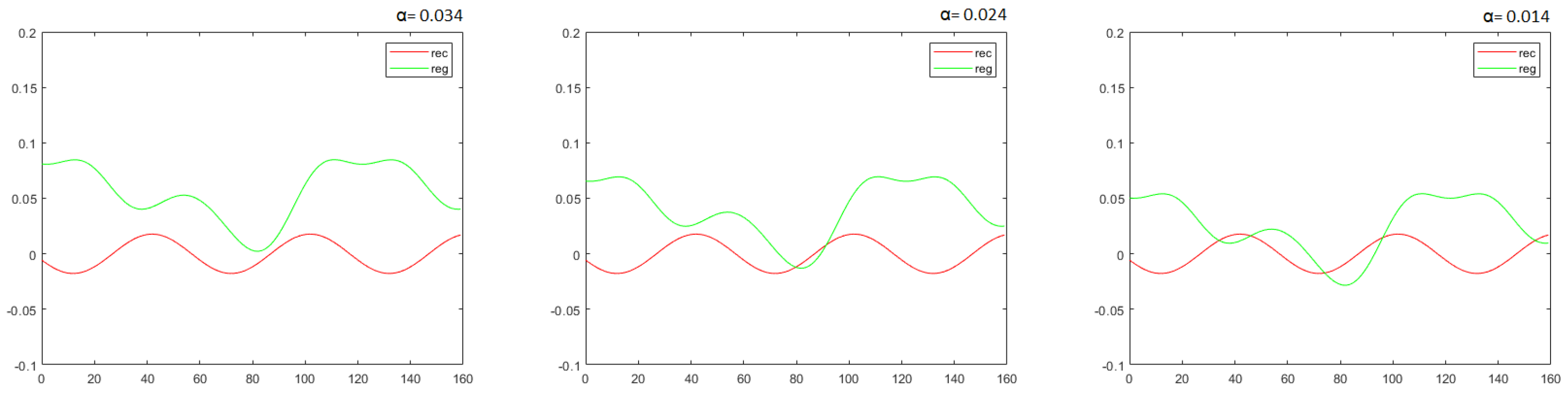
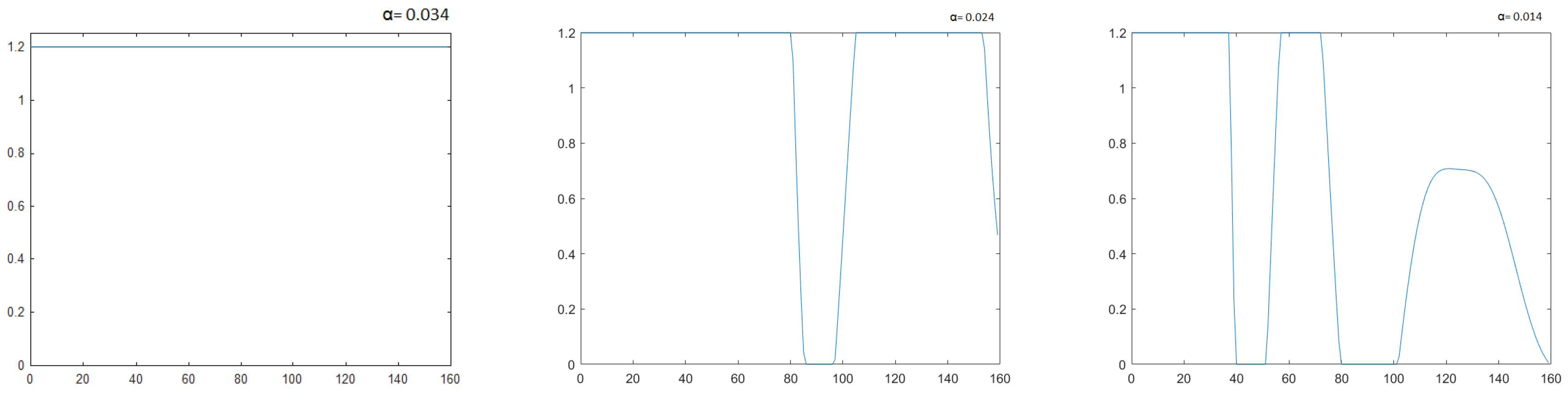
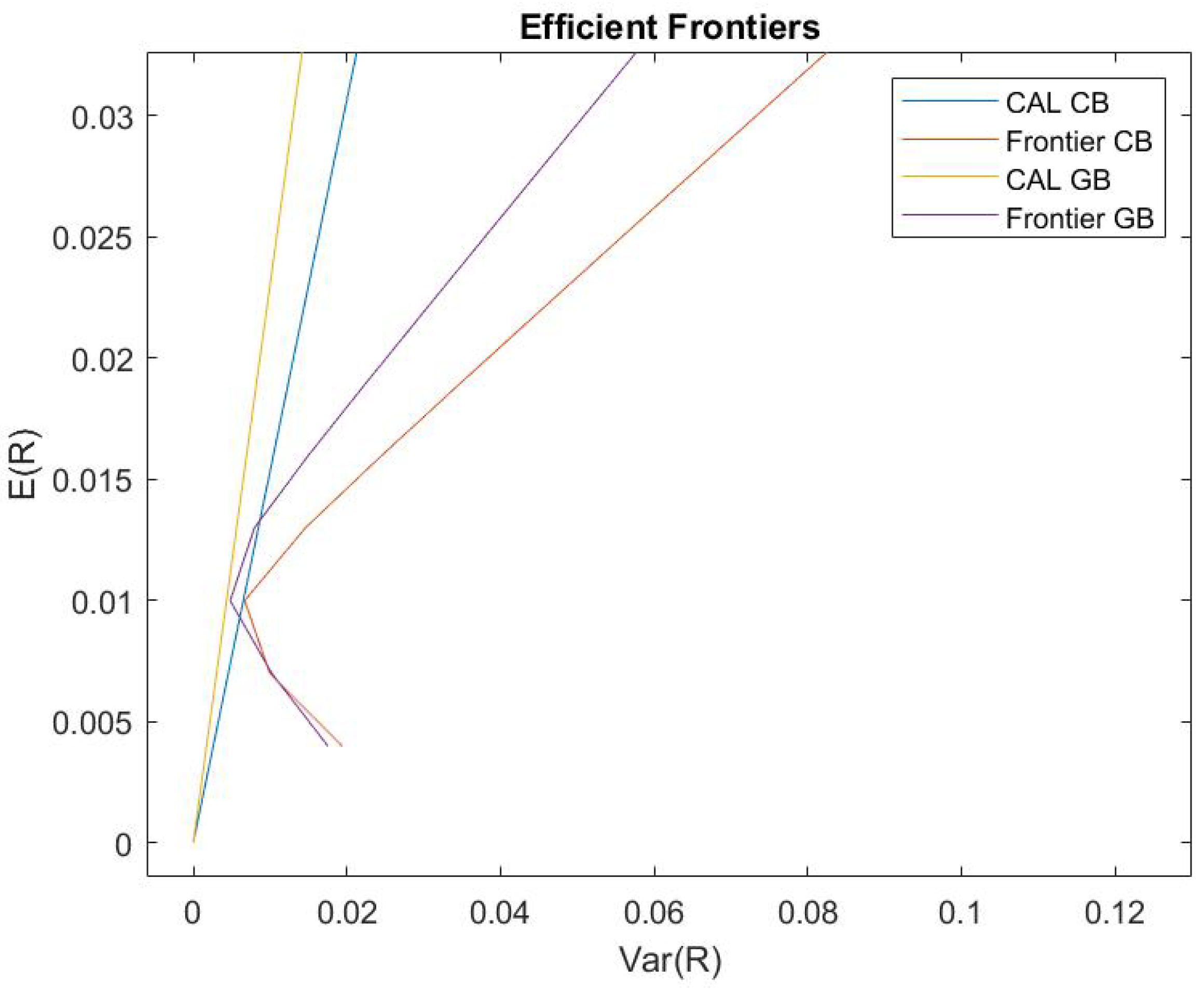
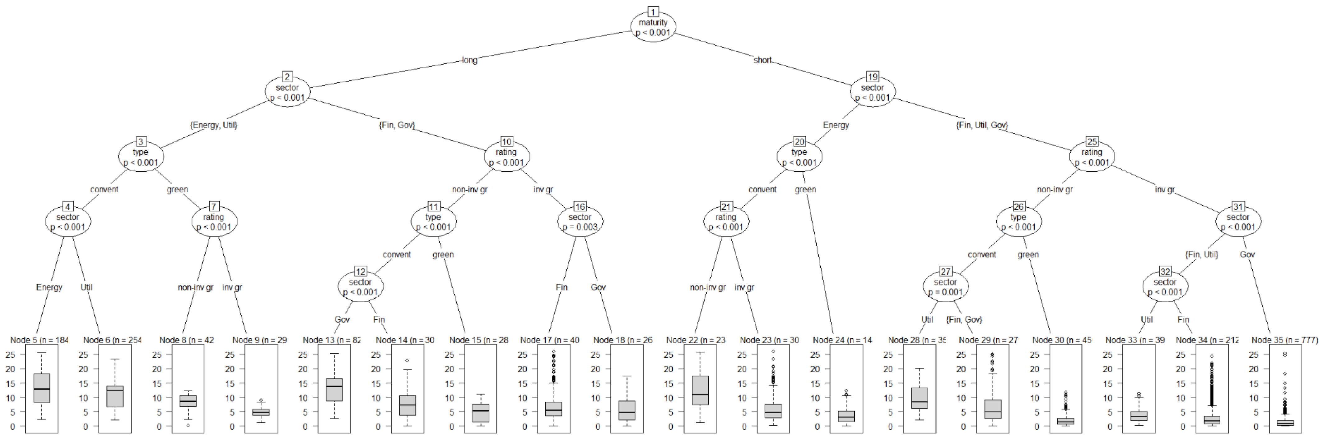
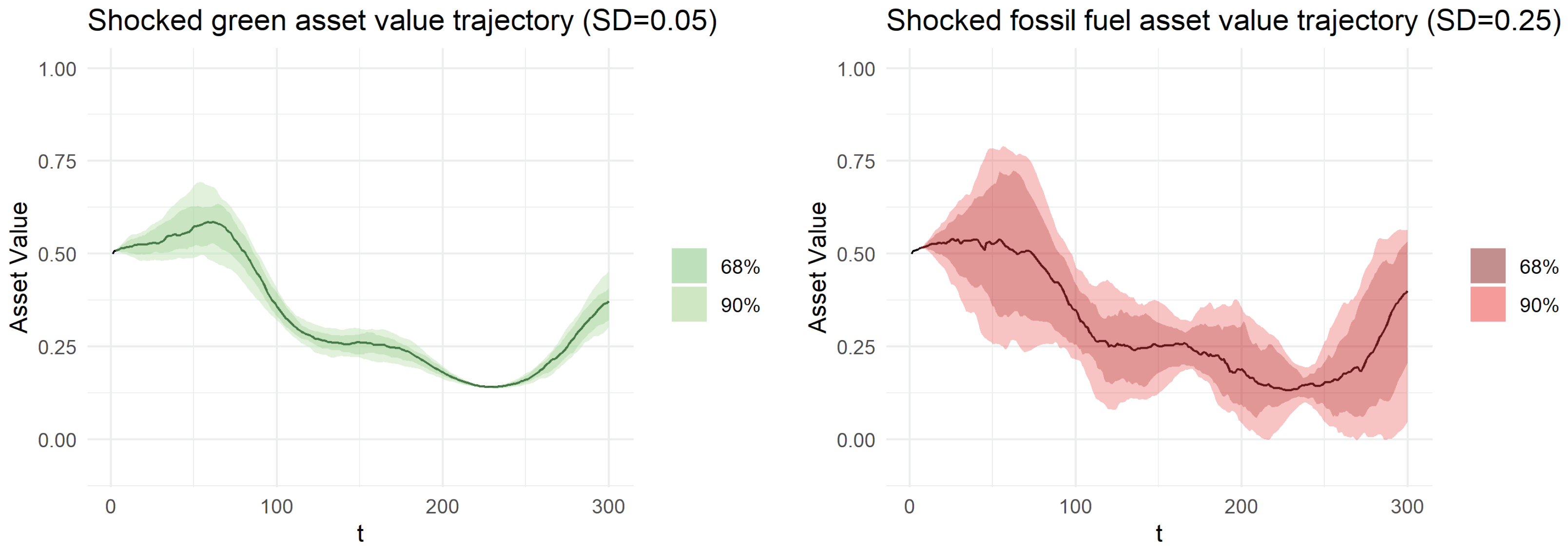
Table A1.
Analysis 1a—Multivariate regression yield at issue.
| Dependent Variable: Yield at Issue | ||||
|---|---|---|---|---|
| (1) Base Model | (2) Sector Model | (3) USD Model | (4) EUR Model | |
| Intercept | *** | *** | *** | |
| Green bond (dummy) | *** | *** | *** | |
| Corp sector: energy (dummy) | ||||
| Corp sector: utilities (dummy) | *** | *** | ||
| Government sector (dummy) | *** | ** | ||
| R2 | ||||
| Adj. R2 | ||||
| Num. obs. | 2969 | 2969 | 1794 | 144 |
Standard errors are heteroskedasticity robust. *** ; ** ; * . Note: The table shows regression results for yield at issue rate for green and conventional bonds. The green dummy is 1 if a bond is green and 0 otherwise. The baseline sector for models (2), (3), and (4) is corp sector: finance. Non-depicted regressors include maturity (long-term dummy), S&P rating, coupon rate, amount issued in bn USD, and debt to assets ratio. Results are computed using R 4.0.3 (R Core Team 2020). Fully reproducible code from the authors is available upon request.
Table A2.
Analysis 1b—Multivariate regression for yield to maturity.
| Dependent Variable: YIELD to Maturity | ||||
|---|---|---|---|---|
| (1) Base Model | (2) Sector Model | (3) USD Model | (4) EUR Model | |
| Intercept | *** | *** | *** | *** |
| Green bond (dummy) | * | ** | ** | |
| Volatility 90d | *** | *** | *** | * |
| Corp sector: energy (dummy) | *** | * | * | |
| Corp sector: utilities (dummy) | *** | *** | *** | |
| Government sector (dummy) | *** | *** | * | |
| R2 | ||||
| Adj. R2 | ||||
| Num. obs. | 4454 | 4454 | 2433 | 1739 |
Standard errors are heteroskedasticity robust. *** ; ** ; * . Note: The table shows regression results for yield to maturity rate for green and conventional bonds. The green dummy is 1 if a bond is green and 0 otherwise. The baseline sector for models (2), (3), and (4) is corp sector: finance. Non-depicted regressors include, again, maturity (long-term dummy), S&P rating, coupon rate, amount issued in bn USD, debt to assets ratio, as well as the bid-ask spread and quarterly dummies from 2017 Q2 until 2020 Q2. Results are computed using R 4.0.3 (R Core Team 2020). Fully reproducible code from the authors is available upon request.
(2) Bond-paired yield regressions, as in Section 4.3:
Instead of using the green minus conventional (GMC) SRb, we use GMC bond yields as the main dependent variable. The aggregate results of our paired subset of data confirm the findings of Kapraun and Scheins (2019), which is a negative green premium for yield at issue rates but a positive green premium (“greenium”) for yield to maturity rates in comparison to conventional bonds (see Table A4). In line with the literature, we also find that institutional bond issuers reflect a negative green yield effect, as the dummy variable for the government sector is significantly negative for all cases (see models 2–4 in Table A4). For the yield at issue regression, we mostly find no significant effect of the green dummy, except for for the base regression case, where a weakly positive yield difference is reported (see Table A3). However, due to the lack of observations, it was not possible to control for all sectors or add a model for EUR bonds, which means that the outcome of the regression should not be over interpreted.
Table A3.
Analysis 2a—Paired bond regression results for yield at issue.
| Dependent Variable: Yield at Issue | |||
|---|---|---|---|
| (1) Base Model | (2) Sector Model | (3) USD Model | |
| Constant (green premium) | * | ||
| Government Sector (dummy) | |||
| R2 | |||
| Adj. R2 | |||
| Num. obs. | 115 | 50 | 47 |
Standard errors are heteroskedasticity robust. *** ; ** ; * . Note: The table shows regression results for yield at issue rates for paired green and conventional bonds. The green dummy is 1 if a bond is green and 0 otherwise. The baseline sector for models (2) and (3) is corp sector: finance. Non-depicted regressors include GMC amount issued, GMC time to maturity, and S&P rating. Results are computed using R 4.0.3 (R Core Team 2020). Fully reproducible code from the authors is available upon request.
Table A4.
Analysis 2b—Paired bond regression results for yield to maturity.
| Dependent Variable: Yield to Maturity | ||||
|---|---|---|---|---|
| (1) Base Model | (2) Sector Model | (3) USD Model | (4) EUR Model | |
| Constant (green premium) | *** | *** | ||
| GMC Volatility 90d | * | |||
| Corp Sector: Energy (dummy) | ** | *** | ||
| Corp Sector: Utilities (dummy) | *** | * | ** | |
| Government Sector (dummy) | *** | ** | *** | |
| R2 | ||||
| Adj. R2 | ||||
| Num. obs. | 304 | 304 | 116 | 176 |
Standard errors are heteroskedasticity robust. *** ; ** ; * . Note: The table shows regression results for yield to maturity rates for paired green and conventional bonds. The green dummy is 1 if a bond is green and 0 otherwise. The baseline sector for models (2) and (3) is corp sector: finance. Non-depicted regressors include GMC amount issued, GMC time to maturity, S&P rating, GMC coupon rate, as well as GMC bid-ask spread. Results are computed using R 4.0.3 (R Core Team 2020). Fully reproducible code from the authors is available upon request.
| 1 | For example, short-termism in the financial market has been shown to be a roadblock; see Davies et al. (2014), Semmler et al. (2020). |
| 2 | For a survey, see Semmler et al. (2021). |
| 3 | However, one should note that there are still methodological challenges related to information asymmetry on the pricing externality effects of conventional and green financial assets (Berg et al. 2019; Candelon et al. 2021a). |
| 4 | In economics, harmonic estimations can capture the business cycle feature of prices, industrial production, employment, and asset returns. For the potential application of harmonic estimations, see Artis et al. (2007). |
| 5 | Respectively, the Bloomberg Barclays MSCI US Global Green Bond in USD (GBUSTRUU) and the Bloomberg Barclays US Corporate Energy in USD (I00388US). |
| 6 | The harmonic estimations are obtained using a FFT. As described in Appendix A, we first de-trend the time series for the real asset returns, and then we are able to apply the FFT in order to filter out short-term movements by estimating the coefficients for a linear combination of a sine–cosine function, based on the original data. The harmonic regression model is estimated for six different frequencies. We select the estimation with the lowest sum of squared errors. |
| 7 | Note that, in order to avoid additional state variables defining stocks of innovation capacity, we undertake a shortcut and let the respective innovations be driven by the respective fraction of wealth. Simulations could be undertaken with various fractions of . |
| 8 | We also want to note that the weights and ) of the two parts of the objective functions in Equations (3) and (5) can be varied, and some Pareto frontier can be computed to explore which weights are the realistic ones (see Kaya and Maurer 2014). |
| 9 | Risk aversion and discount rates have been explored in terms of their relevance to portfolio dynamics in chapters 4–5 in Chiarella et al. (2016). |
| 10 | See Davies et al. (2014) for a discussion of stranded assets. |
| 11 | For details, see (Cochrane et al. 2001, chp. 19), where the bond price is solved for solving the appropriate discount rate forward. In the portfolio context, see (Semmler 2011, chp. 17.5). |
| 12 | It might help to support green start-up firms, ensuring a minimum return if the business does not succeed but high returns if it does. If we think in terms of green treasury bonds, it can help to reduce sovereign debt due to debt to equity swaps. |
| 13 | Both indices were also used for the harmonic estimations and the portfolio model. |
| 14 | It would be ideal for the analyis of long-term bonds to work with a longer trajectory of data. However, the market of green bonds is still new and developing, and due to these market limitations, as well as to constraints in the data availability, we decided to work with data from the period of January 2017 to October 2020. |
| 15 | We abbreviate volatility measures for these 30-, 90-, and 260-day ranges by writing 30d, 90d, and 260d, respectively. |
| 16 | In our empirical analysis, we compared the bond-specific Sharpe ratio results with and without the risk-free rate for the two most frequent currencies (USD and EUR), and did not find a relevant change (differences in the size of the second or the third digit after the decimal). Hence, for simplicity, we do not consider the risk-free rate in our analysis when reporting results on the bond-specific Sharpe ratio SRb. |
| 17 | Even though the formal computation of the RSRL does not require computing the efficient frontier first, Candelon et al. (2021b) used efficient portfolio returns in the computation of the RSRL to connect their analysis to the real estate literature. |
| 18 | YAI values showed few outliers and only observations above the 99th percentile were truncated. In terms of YTM observations, values below the 2.5th percentile and above the 97.5th percentile were truncated. The SRb was calculated based on the filtered YTM and volatility values and outliers below the 2.5th percentile and above the 97.5th percentile were truncated. |
| 19 | e.g., the bond price volatility variable only appears in YTM regressions since YAI is the recorded bond yield at the time of bond issuance and its value is arguably not dependent on bond price changes of the more recent past, and SRb already includes information on bond volatility in its denominator. |
| 20 | In order to reduce the impact of outliers, bid-ask spread observations below the 1st and above the 99th percentile were truncated. |
| 21 | We define long-term bonds similar to Kapraun and Scheins (2019), who categorize them as bonds with a maturity structure of more than ten years (or, see https://www.thebalance.com/choosing-bond-fund-term-416948 (accessed on 18 September 2021)). Our non-long-term bonds include bonds with a maturity structure of 10 years or less and subsume short-term and intermediate-term bonds. In order to reduce the influence of outliers, we excluded observations with a maturity structure of more than 100 years. |
| 22 | In order to reduce the impact of outliers, coupon rate observations below the 1st and above the 99th percentile were truncated. |
| 23 | In order to reduce the impact of outliers, amount issued observations above the 97.5th percentile were truncated. |
| 24 | Since the subset of bonds for the energy sector offers less observations than our total sample, we reduced the date issued control from a year-quarter combination to a yearly dummy. |
| 25 | Our energy-specific subset of data did not have enough observations to run regressions with the YAI rate. |
| 26 | Of course, as Kapraun and Scheins (2019) also argue, once the bonds are traded, there might be a multiplicity of drivers of actual bond prices and yields; for example, relevant are the actual activities in portfolio management, monetary policy and interest rates, varying risk premia, and also for other assets, the varying Distance to Default, and more. |
| 27 | For a further discussion of the utility of convertible bonds, see Section 5.2 of the WB report of Semmler et al. (2021) |
| 28 | The new parameters are set as follows: = 0.9; ; . |
| 29 | We carried out all analyses with all three different volatility measures, but for the matter of simplicity (and unless specified, as in the case of analysis 4 on the energy sector), we only report regressions with the 90-day volatility measure. Results for the different volatility measures are similar and are available upon request. In order to reduce the impact of outliers, the 90d volatility observations above the 95th percentile were truncated. |
References
- Ardia, David, and Kris Boudt. 2015. Testing equality of modified Sharpe ratios. Finance Research Letters 13: 97–104. [Google Scholar] [CrossRef]
- Acemoglu, Daron, Philippe Aghion, Leonardo Bursztyn, and David Hemous. 2012. The environment and directed technical change. American Economic Review 102: 131–66. [Google Scholar] [CrossRef] [PubMed] [Green Version]
- Artis, Michael J., José G. Clavel, Mathias Hoffmann, and Dilip Nachane. 2007. Harmonic regression models: A comparative review with applications Working paper series. Institute for Empirical Research in Economics 2007: 333. [Google Scholar]
- Bachelet, Maria J., Leonardo Becchetti, and Stefano Manfredonia. 2019. The Green Bonds Premium Puzzle: The Role of Issuer Characteristics and Third-Party Verification. Sustainability 11: 1098. [Google Scholar] [CrossRef] [Green Version]
- Barro, Robert J., and Xavier I. Sala-i-Martin. 2004. Economic Growth. Cambridge and London: The MIT Press. [Google Scholar]
- Berg, Florian, Julian F. Koelbel, and Roberto Rigobon. 2019. Aggregate Confusion: The Divergence of ESG Ratings. Cambridge: MIT Sloan School of Management. [Google Scholar]
- Campbell, John Y., and Luis M. Viceira. 2002. Strategic Asset Allocation: Portfolio Choice for Long-Term Investors (Clarendon Lectures in Economics). Oxford: Oxford University Press. [Google Scholar]
- Candelon, Bertrand, Jean-Baptiste Hasse, and Quentin Lajaunie. 2021a. ESG-Washing in the Mutual Funds Industry? From Information Asymmetry to Regulation. Risks 9: 199. [Google Scholar] [CrossRef]
- Candelon, Bertrand, Franz Fuerst, and Jean-Baptiste Hasse. 2021b. Diversification potential in real estate portfolios. International Economics 166: 126–39. [Google Scholar] [CrossRef]
- Chiarella, Carl, Willi Semmler, Chih-Ying Hsiao, and Lebogang Mateane. 2016. Sustainable Asset Accumulation. and Dynamic Portfolio Decisions. Berlin/Heidelberg: Springer. [Google Scholar]
- Cochrane, John H. 2001. Asset Pricing. Princeton: Princeton University Press. [Google Scholar]
- Davies, Richard, Andrew G. Haldane, Mette Nielsen, and W. Silvia Pezzini. 2014. Measuring the costs of short-termism. Journal of Financial Stability 12: 25. [Google Scholar] [CrossRef]
- Ehlers, Torsten, and Frank Packer. 2017. Green bond finance and certification. BIS Quarterly Review 2017: 89–104. [Google Scholar]
- Engle, Robert F., Stefano Giglio, Bryan Kelly, Heebum Lee, and Johannes Stroebel. 2020. Hedging climate change news. The Review of Financial Studies 33: 1184–216. [Google Scholar] [CrossRef]
- Favre, Laurent, and José-Antonio Galeano. 2002. Mean-modified value-at-risk with hedge funds. The Journal of Alternative Investments 5: 21–25. [Google Scholar] [CrossRef]
- Flammer, Caroline. 2021. Corporate green bonds. Journal of Financial Economics 142: 499–516. [Google Scholar] [CrossRef]
- Gregoriou, Greg, and Jean-Pierre Gueyie. 2003. Risk-adjusted performance of funds of hedge funds using a modified Sharpe ratio. The Journal of Wealth Management 6: 77–83. [Google Scholar] [CrossRef]
- Gregory, Aidan. 2020. “Nascent” Green Convertible Bond Market Is Cause for Optimism. Global Capital. July 23. Available online: https://www.globalcapital.com/article/28mu9tpjsiu015prdxb7k/equity-linked/nascent-green-convertible-bond-market-is-cause-for-optimism (accessed on 20 September 2020).
- Greiner, Alfred, Willi Semmler, and Gang Gong. 2005. The Forces of Economic Growth. Princeton: Princeton University. [Google Scholar] [CrossRef] [Green Version]
- Gruene, Lars, Willi Semmler, and Marleen Stieler. 2015. Using nonlinear model predictive control for dynamic decision problems in economics. Journal of Economic Dynamics and Control 60: 112–33. [Google Scholar] [CrossRef] [Green Version]
- Hachenberg, Britta, and Dirk Schiereck. 2018. Are green bonds priced differently from conventional bonds? Journal of Asset Management 19: 371–83. [Google Scholar] [CrossRef]
- Hall, Bronwyn H., Jacques Mairesse, and Pierre Mohnen. 2010. Measuring the Returns to R&D. Handbook of the Economics of Innovation 2: 1033–82. [Google Scholar]
- Han, Yingwei, and Jie Li. 2022. Should investors include green bonds in their portfolios? Evidence for the USA and Europe. International Review of Financial Analysis 80: 1057–5219. [Google Scholar] [CrossRef]
- Hasse, Jean-Baptiste. 2021. DiversificationR: Econometric Tools to Measure Portfolio Diversification. R Package. Available online: https://cran.r-project.org/web/packages/DiversificationR/index.html (accessed on 15 January 2022).
- Hothorn, Torsten, Kurt Hornik, Carolin Strobl, and Achim Zeileis. 2021. Party: A Laboratory for Recursive Partytioning. R Package Version 1.3-7. Available online: https://CRAN.R-project.org/package=party (accessed on 8 May 2021).
- Huynh, Thanh, and Ying Xia. 2021. Climate change news risk and corporate bond returns. Journal of Financial and Quantitative Analysis 56: 1985–2009. [Google Scholar] [CrossRef]
- Immel, Moritz Immel, Britta Hachenberg, Florian Kiesel, and Dirk Schiereck. 2020. Green bonds: Shades of green and brown. Journal of Asset Management 22: 96–109. [Google Scholar] [CrossRef]
- Jones, Benjamin F., and Lawrence H. Summers. 2020. A Calculation of the Social Returns to Innovation. No w27863. National Bureau of Economic Research. Available online: https://www.nber.org/papers/w27863 (accessed on 8 May 2021).
- Kaya, C. Yalcin, and Helmut Maurer. 2014. A numerical method for nonconvex multi-objective optimal control problems. Computational Optimization and Applications 57: 685–702. [Google Scholar] [CrossRef]
- Kapraun, Julia, and Christopher Scheins. 2019. (In)-Credibly Green: Which Bonds Trade at a Green Bond Premium? SSRN Electronic Journal. [Google Scholar] [CrossRef]
- Ledoit, Oliver, and Michael Wolf. 2008. Robust performance hypothesis testing with the Sharpe ratio. Journal of Empirical Finance 15: 850–9. [Google Scholar] [CrossRef] [Green Version]
- Leibowicz, Benjamin D. 2018. Welfare improvement windows for innovation policy. Research Policy 47: 390–98. [Google Scholar] [CrossRef]
- Lintner, John. 1965. Security prices, risk, and maximal gains from diversification. The Journal of Finance 20: 587–615. [Google Scholar]
- Löffler, Kristin Ulrike, Aleksandar Petreski, and Andreas Stephan. 2021. Drivers of green bond issuance and new evidence on the “greenium”. Eurasian Economic Review 11: 1–24. [Google Scholar] [CrossRef]
- MacAskill, Stefen, Eduardo Roca, Benjamin Liu, Rodney Anthony Stewart, and Oz Sahin. 2021. Is there a green premium in the green bond market? Systematic literature review revealing premium determinants. Journal of Cleaner Production 280: 124491. [Google Scholar] [CrossRef]
- Markowitz, Harry. 1952. The utility of wealth. Journal of Political Economy 60: 151–58. [Google Scholar] [CrossRef]
- Merton, Robert C. 1973. An Intertemporal Capital Asset Pricing Model. Econometrica 41: 867887. [Google Scholar] [CrossRef]
- Munk, Claus. 2012. Dynamic Asset Allocation. Lecture Notes. Available online: https://sites.google.com/view/clausmunk/teaching (accessed on 6 June 2021).
- Nisbet, Robert, Gary Miner, and Ken Yale. 2018. Handbook of Statistical Analysis and Data Mining Applications. Amsterdam; Elsevier; Cambridge: Academic Press. [Google Scholar]
- Pham, Linh, and Canh Phuc Nguyen. 2021. How do stock, oil, and economic policy uncertainty influence the green bond market? Finance Research Letters 102128: 1544–6123. [Google Scholar] [CrossRef]
- Piñeiro-Chousa, Juan, M. Ange;es López-Cabarcos, Jerome Caby, and Aleksandar Šević. 2021. The influence of investor sentiment on the green bond market. Technological Forecasting and Social Change 162: 120351. [Google Scholar] [CrossRef]
- R Core Team. 2020. R: A Language and Environment for Statistical Computing. In R Foundation for Statistical Computing. Vienna, Austria: R Core Team, Available online: https://www.R-project.org/ (accessed on 30 October 2021).
- Romer, Paul M. 1986. Increasing returns and long-run growth. Journal of Political Economy 94: 1002–37. [Google Scholar] [CrossRef] [Green Version]
- Semmler, Willi. 2011. Asset Prices, Booms and Recessions: Financial Economics from a Dynamic Perspective. Berlin/Heidelberg: Springer Science & Business Media. [Google Scholar]
- Semmler, Willi, and Chih-Ying Hsiao. 2011. Dynamic Consumption and Portfolio Decisions with Estimated Low Frequency Movements of Asset Returns. The Journal of Wealth Management 14: 101–11. [Google Scholar] [CrossRef]
- Semmler, Willi, K. Lessman, and I. Tahri. 2020. Energy Transition, Asset Price Fluctuations, and Dynamic Portfolio Decisions. Available online: Https://ssrn.com/abstract=3688293 (accessed on 8 May 2021). [CrossRef]
- Semmler, Willi, Joao Paulo Braga, Andreas Lichtenberger, Marieme Toure, and Erin Haider. 2021. Fiscal Policies for a Low-Carbon Economy. Washington, DC: World Bank. [Google Scholar]
- Sharpe, William F. 1964. Capital asset prices: A theory of market equilibrium under conditions of risk. The Journal of Finance 19: 425–42. [Google Scholar]
- Sharpe, William F. 1994. The Sharpe ratio. Journal of Portfolio Management 21: 49–58. [Google Scholar] [CrossRef]
- Tiwari, Aviral Kumar, Emmanuel Joel Aikins Abakah, David Gabauer, and Richard Adjei Dwumfour. 2022. Dynamic spillover effects among green bond, renewable energy stocks and carbon markets during COVID-19 pandemic: Implications for hedging and investments strategies. Global Finance Journal 51: 100692. [Google Scholar] [CrossRef]
- Tobin, James. 1958. Liquidity preference as behavior towards risk. The Review of Economic Studies 25: 65–86. [Google Scholar] [CrossRef]
Figure 1.
Returns for green (reg) and fossil fuel bonds (rec): adjusted harmonic estimations as in Equations (7) and (8).

Figure 2.
Solution paths of wealth for different asset returns; the upper graph with , middle graphs with , and lower graph with (, .
Figure 2.
Solution paths of wealth for different asset returns; the upper graph with , middle graphs with , and lower graph with (, .

Figure 3.
Portfolio decision—share of green assets for the cases with , , and .

Figure 4.
Efficient frontiers of the green bond GBUSTRUU index (GB) and corporate energy I00388US index (CB). The straight lines reflect the respective capital allocation lines (CAL). Efficient frontiers and Markowitz efficient weights are computed in MATLAB 2018b with our own script. Fully reproducible code from the authors is available upon request.

Figure 5.
Analysis 2d—paired bond regression results for bond-specific volatilities (volat).

Figure 6.
Analysis 3—CART results based on the variables and their categories: type (green, conventional (convent)), sectors (energy, finance (Fin), government (Gov), utility (Util)), maturity (long, short), rating (investment-grade (inv gr), non-investment-grade (non-inv gr)). Results are computed using R 4.0.3 (R Core Team 2020) and party (v1.3-7; Hothorn 2021). Fully reproducible code from the authors is available upon request.

Table 1.
Descriptive statistics of collected conventional (CB) and green (GB) bond data issued between 1 January 2017 and 1 October 2020. (Source: Bloomberg terminal).
Table 1.
Descriptive statistics of collected conventional (CB) and green (GB) bond data issued between 1 January 2017 and 1 October 2020. (Source: Bloomberg terminal).
| Categories | CB | GB |
|---|---|---|
| Sectors | ||
| Energy | 809 | 100 |
| Financials | 4822 | 739 |
| Government | 2367 | 271 |
| Utilities | 1028 | 419 |
| Ratings | ||
| A+:A− | 2656 | 118 |
| AAA:AA− | 3310 | 188 |
| B+:B− | 349 | 7 |
| BB+:BB− | 482 | 34 |
| BBB+:BBB− | 1964 | 147 |
| CCC+:D | 136 | 1 |
| Bond duration | ||
| long | 1916 | 266 |
| short | 7011 | 1237 |
| Currencies | ||
| AUD | 525 | 27 |
| BRL | 55 | 46 |
| CAD | 252 | 25 |
| CHF | 147 | 13 |
| CNY | 175 | 157 |
| EUR | 2354 | 355 |
| GBP | 376 | 26 |
| HKD | 210 | 32 |
| IDR | 54 | 5 |
| INR | 58 | 29 |
| Currencies | ||
| JPY | 278 | 70 |
| MXN | 69 | 7 |
| MYR | 1 | 108 |
| Currencies | ||
| NOK | 109 | 36 |
| NZD | 132 | 6 |
| SEK | 232 | 209 |
| TRY | 106 | 11 |
| USD | 3637 | 274 |
| ZAR | 78 | 14 |
| Other | 179 | 79 |
Table 2.
Sharpe ratio comparison based on corporate energy (conventional) and green bond index (green) time series data between 1 January 2017 and 1 October 2020. (Source: MSCI).
Table 2.
Sharpe ratio comparison based on corporate energy (conventional) and green bond index (green) time series data between 1 January 2017 and 1 October 2020. (Source: MSCI).
| Tests | Conventional | Green |
|---|---|---|
| RSRL | 0.7271399 *** | 0.6875913 *** |
| mRSRL | 0.5043868 *** | 0.501156 *** |
Note: Significance levels are *** , ** , * Note: Results are computed using R 4.0.3 (R Core Team 2020) and DiversificationR (v0.1.0; (Hasse 2021)) package, which is available on CRAN. Fully reproducible code from the authors is available upon request.
Table 3.
Multivariate regression for bond-specific Sharpe ratio (SRb).
| Dependent Variable: Bond-Specific Sharpe Ratio (SRb) | ||||
|---|---|---|---|---|
| (1) Base Model | (2) Sector Model | (3) USD Model | (4) EUR Model | |
| Intercept | 0.727 *** | 0.594 *** | 0.851 *** | |
| Green bond (dummy) | 0.603 ** | 0.535 ** | 1.189 * | |
| Corp sector: energy (dummy) | −0.132 *** | −0.165 *** | ||
| Corp sector: utilities (dummy) | −0.100 *** | −0.202 *** | *** | |
| Government sector (dummy) | *** | *** | *** | |
| R2 | ||||
| Adj. R2 | ||||
| Num. obs. | 4028 | 4028 | 2357 | 1532 |
Standard errors are heteroskedasticity robust. *** ; ** ; * . Note: The table shows regression results for the bond-specific Sharpe ratio for green and conventional bonds. The green dummy is 1 if a bond is green and 0 otherwise. The baseline sector for models (2), (3), and (4) is corp sector: finance. Non-depicted regressors include, again, maturity (long-term dummy), S&P rating, coupon rate, amount issued in bn USD, debt to assets ratio, as well as the bid-ask spread, and quarterly dummies from 2017 Q2 until 2019 Q4. Results are computed using R 4.0.3 (R Core Team 2020). Fully reproducible code from the authors is available upon request.
Table 4.
Paired bond regression results for bond-specific Sharpe ratio (SRb).
| Dependent Variable: Bond-Specific Sharpe Ratio (SRb) | ||||
|---|---|---|---|---|
| (1) Base Model | (2) Sector Model | (3) USD Model | (4) EUR Model | |
| Constant (green premium) | *** | ** | * | |
| Corp Sector: Energy (dummy) | ** | ** | ||
| Corp Sector: Utilities (dummy) | ** | |||
| Government Sector (dummy) | *** | |||
| R2 | ||||
| Adj. R2 | ||||
| Num. obs. | 209 | 209 | 113 | 84 |
Standard errors are heteroskedasticity robust. *** ; ** ; * . Note: The table shows regression results for the bond-specific Sharpe ratio for paired green and conventional bonds. The green dummy is 1 if a bond is green and 0 otherwise. The baseline sector for models (2) and (3) is corp sector: finance. Non-depicted regressors include GMC amount issued, GMC time to maturity, S&P rating, GMC coupon rate, as well as GMC bid-ask spread. Results are computed using R 4.0.3 (R Core Team 2020). Fully reproducible code from the authors is available upon request.
Table 5.
Analysis 2d—paired bond regression results for bond-specific volatilities (volat).
| Dependent Variable: Volatilities (30d, 90d, 260d) | |||||||||
|---|---|---|---|---|---|---|---|---|---|
| (1a) | (1b) | (1c) | (2a) | (2b) | (2c) | (3a) | (3b) | (3c) | |
| 30d | 90d | 260d | USD.30d | USD.90d | USD.260d | EUR.90d | EUR.90d | EUR.260d | |
| Constant (Corp Sector: Finance) | *** | * | |||||||
| Corp Sector: Energy (dummy) | * | ** | *** | *** | |||||
| Corp Sector: Utilities (dummy) | * | *** | |||||||
| Gov Sector (dummy) | * | ** | *** | *** | *** | *** | |||
| R2 | |||||||||
| Adj. R2 | |||||||||
| Num. obs. | 413 | 312 | 265 | 125 | 117 | 77 | 190 | 183 | 132 |
Standard errors are heteroskedasticity robust. *** ; ** ; * . Note: Results are computed using R 4.0.3 (R Core Team 2020). Fully reproducible code from the authors is available upon request.
Table 6.
Analysis 4a—Energy sector regression: yield to maturity.
| Dependent Variable: Yield to Maturity | |||||||||
|---|---|---|---|---|---|---|---|---|---|
| (1a) | (1b) | (1c) | (2a) | (2b) | (2c) | (3a) | (3b) | (3c) | |
| 30d | 90d | 260d | USD.30d | USD.90d | USD.260d | EUR.90d | EUR.90d | EUR.260d | |
| Intercept | *** | *** | *** | *** | *** | *** | *** | *** | *** |
| Green bond (dummy) | |||||||||
| Volatility 30d | *** | *** | |||||||
| Green × Volatility 30d | |||||||||
| Volatility 90d | *** | *** | |||||||
| Green × Volatility 90d | * | ||||||||
| Volatility 260d | *** | *** | |||||||
| Green × Volatility 260d | * | *** | |||||||
| R2 | |||||||||
| Adj. R2 | |||||||||
| Num. obs. | 653 | 640 | 534 | 485 | 503 | 386 | 77 | 76 | 70 |
Standard errors are heteroskedasticity robust. *** ; ** ; * . Note: The table shows regression results for yield to maturity rates for green and conventional energy bonds. The green dummy is 1 if a bond is green and 0 otherwise. Non-depicted regressors include maturity (long-term dummy), S&P rating, coupon rate, amount issued in bn USD, debt to assets ratio, as well as bid-ask spread and yearly dummies for 2018 and 2019. Results are computed using R 4.0.3 (R Core Team 2020). Fully reproducible code from the authors is available upon request.
Table 7.
Analysis 4b—Energy sector regression: bond-specific Sharpe ratio (SRb).
| Dependent Variable: Bond-Specific Sharpe Ratio (SRb) | |||||||||
|---|---|---|---|---|---|---|---|---|---|
| (1a) | (1b) | (1c) | (2a) | (2b) | (2c) | (3a) | (3b) | (3c) | |
| 30d | 90d | 260d | USD.30d | USD.90d | USD.260d | EUR.90d | EUR.90d | EUR.260d | |
| Intercept | *** | *** | * | *** | *** | *** | ** | ** | |
| Green bond (dummy) | * | * | * | ||||||
| R2 | |||||||||
| Adj. R2 | |||||||||
| Num. obs. | 650 | 637 | 528 | 485 | 503 | 386 | 75 | 73 | 67 |
Standard errors are heteroskedasticity robust. *** ; ** ; * . Note: The table shows regression results for the bond-specific Sharpe ratio for green and conventional energy bonds. The green dummy is 1 if a bond is green and 0 otherwise. Non-depicted regressors include maturity (long-term dummy), S&P rating, coupon rate, amount issued in bnUSD, debt to assets ratio, as well as bid-ask spread and yearly dummies for 2018 and 2019. Results are computed using R 4.0.3 (R Core Team 2020). Fully reproducible code from the authors is available upon request.
Publisher’s Note: MDPI stays neutral with regard to jurisdictional claims in published maps and institutional affiliations. |
© 2022 by the authors. Licensee MDPI, Basel, Switzerland. This article is an open access article distributed under the terms and conditions of the Creative Commons Attribution (CC BY) license (https://creativecommons.org/licenses/by/4.0/).
Share and Cite
MDPI and ACS Style
Lichtenberger, A.; Braga, J.P.; Semmler, W. Green Bonds for the Transition to a Low-Carbon Economy. Econometrics 2022, 10, 11. https://0-doi-org.brum.beds.ac.uk/10.3390/econometrics10010011
AMA Style
Lichtenberger A, Braga JP, Semmler W. Green Bonds for the Transition to a Low-Carbon Economy. Econometrics. 2022; 10(1):11. https://0-doi-org.brum.beds.ac.uk/10.3390/econometrics10010011
Chicago/Turabian StyleLichtenberger, Andreas, Joao Paulo Braga, and Willi Semmler. 2022. "Green Bonds for the Transition to a Low-Carbon Economy" Econometrics 10, no. 1: 11. https://0-doi-org.brum.beds.ac.uk/10.3390/econometrics10010011
Note that from the first issue of 2016, this journal uses article numbers instead of page numbers. See further details here.