The Age–Period–Cohort Problem in Hedonic House Prices Models

Abstract

The age–period–cohort problem has been studied for decades but without resolution. There have been many suggested solutions to make the three effects estimable, but these solutions mostly exploit non-linear specifications. Yet, these approaches may suffer from misspecification or omitted variable bias. This paper is a practical-oriented study with an aim to empirically disentangle age–period–cohort effects by providing external information on the actual depreciation of housing structure rather than taking age as a proxy. It is based on appraisals of the improvement values of properties in New Zealand to estimate the age-depreciation effect. This research method provides a novel means of solving the identification problem of the age, period, and cohort trilemma. Based on about half a million housing transactions from 1990 to 2019 in the Auckland Region of New Zealand, the results show that traditional hedonic prices models using age and time dummy variables can result, ceteris paribus, in unreasonable positive depreciation rates. The use of the improvement values model can help improve the accuracy of home value assessment and reduce estimation biases. This method also has important practical implications for property valuations.

1. Introduction

The hedonic price method, also known as hedonic regression, has been extensively used in real estate and urban economics research over the past forty or fifty years1. Some of these applied areas include the adjustment for quality in constructing a housing price index, mass valuation of properties, the analysis of demand for urban and housing characteristics, and the testing of assumptions in spatial economics. The fundamental idea of the hedonic price method is to decompose the implicit value of quality features that a commodity has and to summarize the estimated values of those separate properties to characterize the aggregate value. Rosen (1974) was the first scholar to formulate the hedonic price method into standard economic theory by deriving ‘bid functions’ of utility maximizing consumers and ‘offer functions’ of profit-maximizing producers to prove a state of equilibrium for the hedonic price function. However, a major empirical but not yet resolved issue pertaining to the hedonic price method is the age–period–cohort (APC) problem. The APC problem is most commonly dealt with by omitting one of the three variables. However, this approach fails to solve the estimation problem and instead causes a biased estimate of coefficients, as shown below.

To simplify the derivation, suppose the true price, $V_i$, of house $i$ is estimated by Equation (1):

$$V_i={\alpha }_0+{\alpha }_1{A}_i+{\beta }_1{P}_i+{\gamma }_1{C}_i+{\epsilon }_i$$

(1)

Owing to the exact collinearity issue among age, $A_i$, period, $P_i$, and cohort, $C_i$ variables, researchers commonly omit the cohort variable $C_i$ and have adapted Equation (2) to estimate a hedonic regression:

$$V_i={\alpha }_0{}^{*}+{\alpha }_1{}^{*}{A}_i+{\beta }_1{}^{*}{P}_i+{\epsilon }_i{}^{*}$$

(2)

The estimated ${\alpha }_1{}^{*},{\beta }_1{}^{*}$ thus measure the marginal effect of $A_i$ on $V_i$ and $P_i$ on $V_i$ without holding $C_i$ constant. Since $C_i$ is in the error term, the error term will covary with $A_i$ and $P_i$ if $C_i$ covaries with them. It can be shown that the estimated coefficients ${\alpha }_1{}^{*}$ and ${\beta }_1{}^{*}$ are biased (Kennedy 2003) as follows2:

$$E\left[{\widehat{\alpha }}_1\right]={\alpha }_1+{\beta }_1\frac{Cov\left[A_i,P_i\right]}{Var\left[A_i\right]}+{\gamma }_1\frac{Cov\left[A_i,C_i\right]}{Var\left[A_i\right]}$$

(3a)

$$E\left[{\widehat{\beta }}_1\right]={\beta }_1+{\alpha }_1\frac{Cov\left[A_i,P_i\right]}{Var\left[P_i\right]}+{\gamma }_1\frac{Cov\left[P_i,C_i\right]}{Var\left[P_i\right]}$$

(3b)

These three variables are theoretically considered determinants of house prices because of the impacts of deterioration, inflation, and obsolescence on house prices. It has long been recognized that housing values can be characterized by deteriorating building structures, inflating asset pricing, and obsolete building designs over time. However, these effects are difficult to single out among the contributing attributes, either by the hedonic price model or the repeat-sales method. Almost all previous empirical studies employing the hedonic price or the repeat-sales method have had to omit one of the three variables to make the model estimable. The most common specification of the hedonic price model is to use time dummy variables to estimate house price inflation over time. These attempts either omit age or cohort (year-built) variable. This estimation problem has been coined as an age–period–cohort3 (APC) problem.

In extreme cases, age, period, and cohort can be perfectly collinear, and the regression model cannot be estimated by means of any statistical manipulations. To make it estimable, various solutions have been suggested in past decades. These solutions are reviewed in the ensuing section. However, there are two significant shortcomings in their solutions. First, since they do not have any a priori information on the actual separate effects of the age–period–cohort APC, there is no way to tell whether their approaches are promising or not. Second, since they take age as a proxy of deterioration, their methods cannot reflect changes in housing conditions, such as renovations or rehabilitations. Francke and Minne (2017) is probably the only exception. But these authors tried to separate the structure value from the land value by using the reconstruction cost, which does not reflect the actual conditions of the houses.

This study is one of the original attempts to disentangle the APC effects on house prices by using a direct measure of the deterioration of the physical housing structure instead of taking age as a proxy. We contend that the APC problem is rooted in the use of age, time, and cohort variables as proxies rather than the direct measurement of deterioration, inflation, and obsolescence. We argue that when one of the proxies is replaced by a direct measure of the underlying value, the APC effects can be disentangled. In this study, we took a practical-oriented approach by exploiting the appraised improvement values of housing as a direct indicator of the depreciation/appreciation due to the changes in the physical conditions of the structures. This approach is novel in tackling omitted variable bias of APC effects on housing prices. It requires detailed data on the improvement values of all houses to enable this approach to be feasible.

This paper is structured as follows. In Section 2, we review the literature on the APC trilemma in real estate. In Section 3, we discuss the research design, and in Section 4, we present the data and discuss the empirical results. In Section 5, we conclude with the findings and implications of the study.

2. Literature Review

The APC trilemma is common in demography, epidemiology, sociology, biostatistics, and financial analyses (Bosman 2012; de Vaus 2001; Keyes et al. 2010; Mason and Wolfinger 2001; Smith 2008; Yang and Land 2008; Yang 2010). Hall (1971) first raised the APC problem in real estate research, which refers to the effects of deterioration, inflation, and obsolescence on property prices. However, most studies on the determinants of house prices do not include the cohort effect because in a regression model it can be perfectly collinear with age and period variables. Many scholars have tried various approaches to disentangle the collinearity issue (Chinloy 1977; Englund et al. 1998; Palmquist 1979; Quigley 1995). Their efforts can be categorized into three approaches, as reviewed below. However, these approaches have generated considerable controversies regarding their plausibility (Hobcraft et al. 1985; Rodgers 1982). The inextricably intertwined effects of the elements of APC in additive regression models, most commonly used in hedonic pricing analysis, have resulted in a trilemma whereby only two out of the three variables are estimable (Yiu 2009).

In econometrics, the multicollinearity problem can only be solved by using prior external information (Intriligator et al. 1996; Chau et al. 2005). Yang (2010, p. 21) even concludes that ‘there will never be a solution within the confine of linear models’. The constrained coefficients approach imposes one or more equality constraints on the coefficients of one parameter (Yang 2010). For example, in almost all the previous hedonic pricing analyses that have been applied in housing studies, the cohort effect is ignored, and a linear age effect is assumed. Sometimes, this produces a counterintuitive result such as a positive age effect (Clapp and Giaccotto 1998; Gallimore et al. 1996), which contradicts the common understanding of deterioration and the ‘premium for newness’ as discussed in Rubin (1993). Gallimore et al. (1996) conjecture that such counterintuitive results are caused by housing quality issues, and Clapp and Giaccotto (1998) argue that the positive age effect is due to the excess demand for particular age-related locations. However, age coefficient estimates have been biased by the omitted cohort variable and the neglect of renovation/rehabilitation values.

The non-linear parametric transformation approach applies a non-linear parametric function for at least one of the APC variables. For example, some scholars have tried to estimate non-linear age effects (Cannaday et al. 2005; Denton et al. 1999; Waddell et al. 1996). A non-linear age or cohort effect may help achieve an estimable hedonic analysis, but it does not provide evidence that the selected non-linear functional form is justified. For example, Coulson and McMillen (2008) use a non-parametric approach developed by McKenzie (2006) to estimate a U-shaped age effect, but they provide no validation of the results. This paper, in contrast, verified the cohort effects based on a priori market information of the housing quality issues of specific cohorts.

The building cohort effect is considered to be the result of certain architectural or building qualities associated with the structures built at a specific period, whereby buyers are willing to pay a premium to enjoy such architectural or structure qualities attached to the particular cohort. For example, heritage value can be regarded as a cohort effect of historic houses. O’Brien (2011) argues that the APC formulation fails to differentiate two fundamental problems: (1) the complete confounding of the linear effects of age with the effects of period and cohort, and (2) the problem of model identification.4 This trilemma can be illustrated by the following identity: The cohort ($\kappa$) of a house is equivalent to the difference between the transaction period ($\pi$) and the age ($\alpha$) of property i, that is, ${\kappa }_i\equiv {\pi }_i-{\alpha }_i$.

For instance, if a house that is 20 years old (${\alpha }_i=20$) is transacted in the year 2020 (${\pi }_i=2020$), then it must have been built in the year 2000 (${\kappa }_i=2000$). In theory, unless additional external information is provided, the complete confounding linear effects of either cohort with age and period, age with period and cohort, or period with age and cohort, renders the estimation of the simultaneous APC effect on house prices impossible. According to O’Brien’s (2011), it is impossible to set the constraints that are consistent with the data-generating process.5 In real estate markets, disentangling the APC effects is essential for investment and policy decision-making, as, in some specific cohorts, there are defective buildings. For example, the “leaky homes crisis” in the 1990s and 2000s in New Zealand (PricewaterhouseCoopers 2009) and the “short pile incidents” in the 2000s in Hong Kong (Hencher et al. 2005) are notorious cases of housing cohorts with deficiencies that adversely affected housing prices. However, a survey of 78 hedonic studies referenced by Sirmans et al. (2006) found that no study had examined all APC effects in the specification.

Nevertheless, in the hope of revealing the three effects correctly, all these studies relied, without reasonable grounds, on a pre-determined functional form. Furthermore, a linear deterioration rate proxied by housing age has been challenged because the quality of houses can be improved by renovation or rehabilitation. For example, Goodman and Thibodeau (1995) found a positive age effect for houses between 20 and 40 years old. Randolph (1988) explained positive effects for older houses by indicating a preference for renovating good quality older properties. Yet, such an explanation is inadequate given that the premium should be consistent with the renovation of good quality properties across cohorts. In this paper, in contrast, we attempt to control the actual deterioration condition by incorporating the assessed improvement value of each transacted house.

3. Research Design

This paper tests several different model specifications to illustrate the APC problem and the multicollinearity issues of various previous solutions. Equation (4) shows the theoretical but non-estimable semi-log hedonic price model due to the exact collinearity among the linear APC variables:

$$ln\left(V_{is}\right)={\alpha }_0+{\alpha }_1{A}_i+{\beta }_1{P}_i+{\gamma }_1{C}_i+{\displaystyle \sum }_{k=1}^K{\pi }_k{X}_{ki}+{\displaystyle \sum }_{s=1}^S{\theta }_s{L}_{is}+{\epsilon }_{is}$$

(4)

where V_is denotes the value of property i, being built at year $C_i$, transacted at year $P_i$ and located at suburb s (i = 1, …, n; s = 1, …, S), A_i denotes the age variable, which equals $P_i-C_i$, thus resulting in exact collinearity among the APC variables; ${\pi }_k$ and ${\theta }_s$ denotes the implicit prices for the k^th property characteristic X_jk (k = 1, …, K) and s^th suburb location dummy L_is (s = 1, …, S), respectively. ε_ist denotes the error term with the mean zero and the variance σ². The coefficients can be estimated by the ordinary least square method.

In order to make the equation estimable, non-linear specifications and/or omitted variable(s) techniques have usually been used. But if all the three variables are transformed into dummy variables of the same frequency, such as yearly dummies $A_{i{t}_y}, P_{i{t}_y},C_{i{v}_y}$, then it will still be perfectly collinear and cannot be estimated (Equation (5)).

$$ln\left(V_{its}\right)={\alpha }_0+{\displaystyle \sum }_{a=0}^{A_y}{\alpha }_a{A}_{i{t}_y}+{\displaystyle \sum }_{t=1}^{T_y}{\beta }_t{P}_{i{t}_y}+{\displaystyle \sum }_{v=1}^{V_y}{\gamma }_v{C}_{i{v}_y}+{\displaystyle \sum }_{k=1}^K{\pi }_k{X}_{ki}+{\displaystyle \sum }_{s=1}^S{\theta }_s{L}_{is}+{\epsilon }_{ist}$$

(5)

Equation (6) transforms the linear period variable into a series of monthly dummies to allow non-linear time effects and keeps age and cohort as linear variables.

$$ln\left(V_{its}\right)={\alpha }_0+{\alpha }_1{A}_i+{\displaystyle \sum }_{t=1}^{T_m}{\beta }_t{P}_{i{t}_m}+{\gamma }_1{C}_i+{\displaystyle \sum }_{k=1}^K{\pi }_k{X}_{ki}+{\displaystyle \sum }_{s=1}^S{\theta }_s{L}_{is}+{\epsilon }_{its}$$

(6)

where $P_{i{t}_m}$denotes the monthly dummy, which is set to 1 if the ith house is sold at time t, and otherwise to 0 (t = 1, …, T).

Equation (7) further transforms both the linear period and cohort variables into two series of non-linear period and cohort dummies in different frequencies to build an estimable hedonic price model, the former by month, and the latter by decade. Yet, the multicollinearity issue of this specification can be expected to be serious.

$$ln\left(V_{its}\right)={\alpha }_0+{\alpha }_1{A}_i+{\displaystyle \sum }_{t=1}^{T_m}{\beta }_t{P}_{i{t}_m}+{\displaystyle \sum }_{v=1}^{V_d}{\gamma }_v{C}_{i{v}_d}+{\displaystyle \sum }_{k=1}^K{\pi }_k{X}_{ki}+{\displaystyle \sum }_{s=1}^S{\theta }_s{L}_{is}+{\epsilon }_{ist}$$

(7)

where $C_{i{v}_d}$ denotes the cohort dummy, which is set to 1 if the ith house was built in decade v, and otherwise to 0 (v = 1, …, V).

Besides using non-linear variables to solve the APC problem, omitting the cohort variable in hedonic price models is more common, as shown in Equation (8). This equation includes a linear age variable and non-linear time dummy variables. However, both the estimated ${\widehat{\alpha }}_1$ and ${\widehat{\beta }}_t$ will be biased due to the omitted cohort variable.

$$ln\left(V_{its}\right)={\alpha }_0+{\alpha }_1{A}_i+{\displaystyle \sum }_{t=1}^{T_m}{\beta }_t{P}_{i{t}_m}+{\displaystyle \sum }_{k=1}^K{\pi }_k{X}_{ki}+{\displaystyle \sum }_{s=1}^S{\theta }_s{L}_{is}+{\epsilon }_{its}$$

(8)

In this study, we have a priori information on cohort effects due to the leaky homes crisis in New Zealand. Timber-framed houses built from 1988 to 2004 fall in the cohorts of leaky homes due to the changes of weather-tightness requirements in the building regulations. Since the quality issue can result in the decay of timber framing, which, in extreme cases, can make buildings structurally unsound, homebuyers have avoided buying houses of these cohorts unless they are certified to have been rectified. Thus, the cohorts of the 1990s and 2000s are expected to have a relatively lower price than those of the 1980s or 2010s, ceteris paribus. The incident provides a refutable implication on the cohort hypothesis rather than just a form of the curve-fitting exercise used in most previous studies. Furthermore, the cohort variables also test historic cohort effects based on the construction and workmanship of the pre-war cohorts. Equation (9) replaces the age variable in Equation (6) by the appraised improvement value of the house before the transaction $I{V}_i$. This is coined as an improvement value–period–cohort (IPC) hedonic price model. The improvement value of each transacted house can be considered a proxy variable of the actual deterioration or renovation effect.6 It not only solves the multicollinearity problem but also introduces the value of renovations or rehabilitations into the hedonic models.

$$ln\left(V_{its}\right)={\alpha }_0+{\alpha }_{2}ln\left(I{V}_{its}\right)+{\displaystyle \sum }_{t=1}^{T_m}{\beta }_t{P}_{i{t}_m}+{\displaystyle \sum }_{v=1}^{V_d}{\gamma }_v{C}_{i{v}_d}+{\displaystyle \sum }_{k=1}^K{\pi }_k{X}_{ki}+{\displaystyle \sum }_{s=1}^S{\theta }_s{L}_{is}+{\epsilon }_{ist}$$

(9)

4. Empirical Data and Results

The models are empirically tested using housing transaction data recorded by Auckland Council, New Zealand, from January 1990 to December 2019 (360 months), which, after all the outliers are excluded, provides about half a million housing transactions. It is one of the biggest housing transaction datasets, which can help exclude any potential estimation problems due to insufficient data. The dataset is not open access but subscribed by the university library from an international property data company: CoreLogic. In addition to Yiu and Cheung (2021), Cheung and Yiu (2022), and many hedonic pricing modeling applications in New Zealand housing market (see details from Fernandez 2019), the major distinction in this study is the use of the variable ‘building age’. Typically, the government’s official data of the district valuation roll includes only the built cohorts in decade of individual properties. The building age variable is usually unavailable from any official property data sources, including the property data we purchased from CoreLogic. Therefore, to examine the APC effects on house prices in this study, we gathered the information of the home-built year from the online property platforms such as OneRoof.co.nz.

Furthermore, to keep housing type and land tenure uniform, the study was confined to freehold house-type transactions through the exclusion from the transaction data of apartment-type housing, vacant sites, and leasehold interests. Houses built before 1900 were also excluded to avoid heritage effects, but they were less than 0.3% of the sample. We also excluded all the transactions after December 2019 to avoid the pandemic effects. The dataset provided a comprehensive list of housing and neighbourhood attributes, besides age, period, and cohort variables. These attributes include numbers of bedrooms and bathrooms, floor area and land area, districts (suburbs), views, and scopes.

Table 1. Descriptive statistics of other variables.

Panel A	Mean	SD.	Min	Max
$\mathrm{Price}\left(\mathrm{NZ}\text{\$}\right),V_i$	490,575.90	446,307.30	11,000.00	9,985,000.00
$\mathrm{Age}\left(\mathrm{years}\right),A_i$	33.25	26.25	0.00	119.00
Improvement Value (NZ$)	191,378.00	156,458.00	0.00	5,710,000.00
Panel B	Count	Percent	Desc: COHORTS
$C_{i,1900s}$	8193	1.52	Houses built in the 1900s
$C_{i,1910s}$	16,455	3.06	Houses built in the 1910s
$C_{i,1920s}$	26,369	4.90	Houses built in the 1920s
$C_{i,1930s}$	13,461	2.50	Houses built in the 1930s
$C_{i,1940s}$	20,307	3.78	Houses built in the 1940s
$C_{i,1950s}$	56,916	10.59	Houses built in the 1950s
$C_{i,1960s}$	75,927	14.12	Houses built in the 1960s
$C_{i,1970s}$	75,895	14.12	Houses built in the 1970s
$C_{i,1980s}$	77,216	14.36	Houses built in the 1980s
$C_{i,1990s}$	98,176	18.26	Houses built in the 1990s
$C_{i,2000s}$	68,764	12.79	Houses built in the 2000s
Fixed Effects	Count
$\mathrm{Suburbs},L_{is}$	265		Suburbs in the Auckland Region
$\mathrm{Months},P_{it}$	360		January 1990–December 2019

shows the summary statistics of the APC-related attributes.

Table 2. The results of regression Equations (6)–(9).

Equations	Equation (6)	Equation (7)	Equation (8)	Equation (9)
Dep. Var.	ln$\left(\mathrm{House}\mathrm{Values}\right),ln\left(V_{its}\right)$
Variables	Coefficients (t-stat)
Age-in-years, $A_i$	0.0019 (0.0002)	−0.0013 (−10.375) ***	−0.0003 (−18.520) ***	-
Period-in-year, $P_i$	-	-	-	-
Cohort year, $C_i$	0.0023 (0.0002)	-	-	-
Dummies of
Period-in-month, $P_{i{t}_m}$	Figure 1 (Mostly Insign.)	Figure 1 (Mostly sign.)	Figure 1 (Mostly sign.)	Figure 1 (Mostly sign.)
Cohort-in-decade
$C_{i,1900}$	-	0.173 (13.180)	-	0.145 (45.239) ***
$C_{i,1910}$	-	0.174 (14.828) ***	-	0.162 (66.048) ***
$C_{i,1920}$	-	0.089 (8.722) ***	-	0.120 (60.181) ***
$C_{i,1930}$	-	0.051 (5.607) **	-	0.119 (48.667) ***
$C_{i,1940}$	-	−0.041 (−5.187) ***	-	0.081 (38.486) ***
$C_{i,1950}$	-	−0.058 (−9.086) ***	-	0.057 (36.513) ***
$C_{i,1960}$	-	−0.071 (−13.803) ***	-	0.034 (23.220) ***
$C_{i,1970}$	-	−0.085 (−21.512) ***	-	0.008 (5.246) ***
$C_{i,1980}$	-	−0.085 (−30.962) ***	-	−0.020 (−14.054) ***
$C_{i,1990}$	-	−0.029 (−16.700) ***	-	−0.013 (−9.980) ***
ln$\left(\mathrm{ImprVal}\right),ln\left(I{V}_{its}\right)$	-	-	-	0.307 (357.027) ***
Centred VIF for Age Variable	UICM	92.018 > 10	1.724 < 10
Centred VIF for Period Variables	UICM	1.612–4.228 All < 10	1.596–4.089 All < 10	1.675–7.020 All < 10
Centered VIF for Cohort Variables	UICM	3.763–41.183 80% > 10		1.376–2.540 All < 10
$\mathrm{Centered}\mathrm{VIF}\mathrm{for}ln\left(I{V}_{its}\right)$				2.639 < 10
No. of Obs.	536,858	536,858	536,858	427,646
Adj. R-Squared	0.871	0.875	0.871	0.898

Notes: The dependent variable ln(V) is the logarithm of the net transacted house prices in New Zealand dollars. $C_{i,1950}$ Cohort-in-decade dummy, **, *** means that the coefficient is significant at the 5%, 1% levels, respectively. Figures in the parentheses are the t-statistics. Outliers of V ≤ $10,000 and V ≥ $10,000,000 are excluded. Apartment type housing, leasehold interests, heritage (C < 1900), and pre-sales (age < 0) are also excluded. UICM stands for unable to invert covariance matrix. 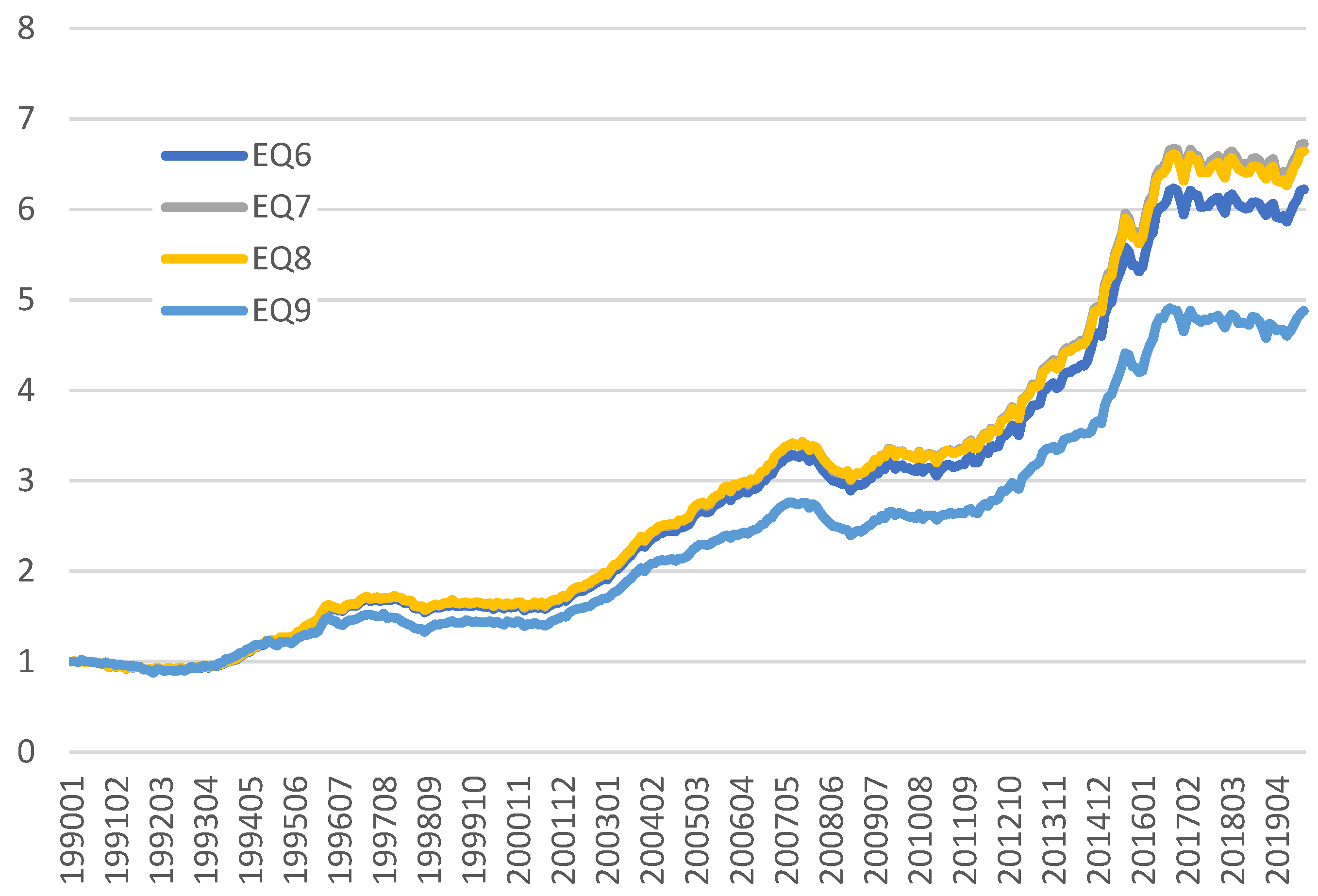x% > 10 refers to x% of the variables that have their VIFs greater than 10.

shows the results. Since Equations (4) and (5) are non-estimable due to perfect collinearity among the three linear APC variables and the three equal-frequency APC dummy variables, respectively, they are not shown in the table. Column (1) shows the result of Equation (6), which converts the period variable into 359 (monthly) period dummies to make it estimable. However, the estimated age effect is positive, which contradicts the expected negative depreciation (Randolph 1988). In addition, the highly similar magnitudes of the age and cohort coefficients and their p-values indicate serious multicollinearity between these variables. Even though the APC coefficients are then estimable, the high insignificance of the estimates renders the results unplausible. The house price index estimated from the period dummies was found to be an overestimate (Figure 1). The coefficients of all the housing characteristics among the models were mostly significant with similar signs and magnitudes as expected7. Column (2) shows the model of a linear age variable and two series of non-linear period dummies by month, and cohort dummies by decade. Most of the results were statistically significant, though the centered variance inflation factors (VIFs) of the age and cohort coefficients far exceeds 10, indicating a severe multicollinearity issue. Further, the estimated age effect (depreciation rate) was negative but unreasonably small at 0.1% per year. There are at least two plausible reasons for this. First, when older houses are renovated or refurbished, the depreciation rate proxied by house age reflects the enhanced value. Second, the leaky home crisis affecting more recent cohorts distorts the estimated depreciation rate proxied by house age.

A priori information of the cohort effects in Auckland is the notorious leaky homes crisis (Rehm et al. 2019). Houses built from 1988 to 2004 fall in the cohorts of leaky homes. However, the cohort coefficients estimated by Equation (7) do not agree with the leaky homes cohorts. The lowest-priced cohorts were the 1960s, 1970s, and 1980s; they were 7.1%, 8.5%, and 8.5% lower in price than the 2000s cohort. The results further support that the estimates are biased. Column (3) shows the most typical hedonic price model (Equation (8)), which omits cohort variable(s) and uses a single linear age variable and a series of period dummies by month. The results were more reasonable, and with most of the variables statistically significant at the 1% level, the model’s explanatory power was also reasonably high (the adjusted R-squared = 87.7%). This is taken as the baseline house price index for comparison in Figure 1. The age effect is negative, reflecting an expected depreciation of house values on older houses. It explains why most of the hedonic price models adopt this omitted variable solution.

Yet, the depreciation rate is even lower at just about 0.03% for houses one year older. Owing to the omission of the cohort variable(s), the estimates of both the age and period variables are biased. The low depreciation rate is likely to be reflecting a combined effect of negative depreciation and positive obsolescence. Column (4) shows the IPC model (Equation (9)), which replaces the age variable with the natural logarithm of the improvement value. The results imply that house prices positively and significantly reflect renovation and rehabilitation effects. A 1% increase in improvement value can bring about a 0.31% increase in house prices, ceteris paribus. The results agree with the leaky homes crisis well. The leaky homes cohorts (the 1980s, 1990s, and 2000s) are the lowest priced cohorts. Furthermore, the house price index estimated by the period dummies coefficients is much less than other indices, as shown in Figure 1. It reflects that when the cohort effect and renovation effect are not controlled in hedonic pricing analysis, the estimated house price index will be biased and overestimated in this example.

The results show that the IPC model is a feasible approach in home value assessment practice, which does not only allow a direct estimate of the renovation and rehabilitation effect but also helps mitigate the APC problem of biased estimates. The signs of the coefficients for pre-1980 cohorts in Column (4) have changed from negative to positive after replacing the age variable with the improvement value variable. They indicate a more plausible result in line with the leaky homes crisis.

5. Conclusions

This paper discusses the issue, in the hedonic price models, of multicollinearity among housing age, transaction period, and housing cohort, which is known as the APC problem, taking the Auckland Region in New Zealand’s housing market as an example. The issue is well recognized, but almost all the previous studies omit one of the three variables and/or transform some of them into non-linear variables to make the model estimable. The consequence is a biased estimation.

The contribution of this paper is twofold. First, we used a high-quality set of data from the housing markets of the Auckland Region, New Zealand, to demonstrate the multicollinearity issue of the APC problem in various hedonic price models and the biased results. Second, we also made an initial attempt to disentangle the APC problem by using external information—the appraised improvement values of the housing structures—to control the renovation and rehabilitation effects. Methodologically, the estimated cohort effects are compared with a priori information on the leaky home cohort (the 1980s, 1990s, and 2000s) discount in New Zealand (Rehm et al. 2019). Because almost all previous solutions on the APC problem did not empirically tell whether the solutions can make a better estimate, our method can be complementary in testing the correctness of the model with a cross-check of the results. The result from our IPC model successfully identifies the leaky homes cohorts’ discounts.

The implications of this study are far-reaching, especially for the practices of property valuation and housing price index construction. Where the current methods of estimating house price indices by hedonic price models are affected by the APC problem, price indices are likely to be overestimated or biased. Without using any a priori information, such as the improvement values used in our study to adjust, the cohort effect will be embedded in the age and period effects that create an upward bias. To determine the pure temporal impacts on property prices in constructing housing price indices, it is essential to single out the cohort effect from the renovation and rehabilitation effects.

With the advancement of Proptech, many online platforms are trading houses based on traditional hedonic price models which do not consider renovation and rehabilitation values, probably due to lack of data. However, governments have become more common to keep records of renovation and rehabilitation works on houses, such as the building consent system in New Zealand and the Home Conditions Reports in the UK. The hedonic model put forward in this study can be practically applied in housing markets to improve the accuracy of the home value assessment and reduce estimation biases. It helps enhance the market efficiency and viability of online instant home buyers.

References

- Bosman, Merijn. 2012. The Potential of Cohort Analysis for Vintage Analysis: An Exploration. Master’s thesis, University of Twente, Enschede, The Netherlands, January 23. [Google Scholar]
- Cannaday, Roger E., Henry J. Munneke, and Tyler T. Yang. 2005. A Multivariate Repeat-Sales Model for Estimating House Price Indices. Journal of Urban Economics 57: 320–42. [Google Scholar] [CrossRef]
- Chau, Kwong Wing, Siu Kei Wong, and Chung Yim Yiu. 2005. Adjusting for Non-Linear Age Effects in the Repeat Sales Index. Journal of Real Estate Finance and Economics 31: 137–54. [Google Scholar] [CrossRef] [Green Version]
- Cheung, Ka Shing, and Chung Yim Edward Yiu. 2022. The Economics of Architectural Aesthetics: Identifying Price Effect of Urban Ambiences by Different House Cohorts. Environment and Planning B: Urban Analytics and City Science. forthcoming. [Google Scholar]
- Chinloy, Peter T. 1977. Hedonic Price and Depreciation Indexes for Residential Housing: A Longitudinal Approach. Journal of Urban Economics 4: 469–82. [Google Scholar] [CrossRef]
- Clapp, John M., and Carmelo Giaccotto. 1998. Residential Hedonic Models: A Rational Expectations Approach to Age Effects. Journal of Urban Economics 44: 415–37. [Google Scholar] [CrossRef]
- Colwell, Peter F., and Gene Dilmore. 1999. Who was first? An examination of an early hedonic study. Land Economics 75: 620–26. [Google Scholar] [CrossRef]
- Coulson, N. Edward, and Daniel P. McMillen. 2008. Estimating time, age and vintage effects in housing prices. Journal of Housing Economics 17: 138–51. [Google Scholar] [CrossRef]
- Court, Andrew. 1939. Hedonic Price Indexes with Automotive Examples. New York: The Dynamics of Automobile Demand, General Motors, pp. 98–119. [Google Scholar]
- de Vaus, David A. 2001. Research Design in Social Research. London: Sage Publications. [Google Scholar]
- Denton, Frank T., Denton C. Mountain, and Byron G. Spencer. 1999. Age, trend, and cohort effects in a macro model of Canadian expenditure patterns. Journal of Business and Economic Statistics 17: 430–43. [Google Scholar]
- Englund, Peter, John M. Quigley, and Christian L. Redfearn. 1998. Improved Price Indexes for Real Estate: Measuring the Course of Swedish Housing Prices. Journal of Urban Economics 44: 171–96. [Google Scholar] [CrossRef] [Green Version]
- Fernandez, Mario A. 2019. A Review of Applications of Hedonic Pricing Models in the New Zealand Housing Market. Auckland: Auckland Council. [Google Scholar]
- Francke, Marc K., and Alex M. van de Minne. 2017. Land, structure and depreciation. Real Estate Economics 45: 415–51. [Google Scholar] [CrossRef]
- Gallimore, Paul, Michael Fletcher, and Matthew Carter. 1996. Modelling the Influence of Location on Value. Journal of Property Valuation and Investment 14: 6–19. [Google Scholar] [CrossRef]
- Goodman, Allen C., and Thomas G. Thibodeau. 1995. Age-related heteroskedasticity in hedonic house price equations. Journal of Housing Research 6: 25–42. [Google Scholar]
- Haas, George Casper. 1922. A Statistical Analysis of Farm Sales in Blue Earth County, Minnesota, as a Basis for Farm Land Appraisal (No. 1693-2016-137481). Available online: https://ageconsearch.umn.edu/record/184329/files/Haas1.pdf (accessed on 13 October 2021).
- Hall, Robert E. 1971. The Measurement of Quality Change from Vintage Price Data. In Price Indexes and Quality Change: Studies in New Methods of Measurement. Edited by Zvi Griliches. Cambridge: Harvard University Press. [Google Scholar]
- Hencher, S. R., J. T. Tyson, and P. Hutchinson. 2005. Investigating substandard piles in Hong Kong. In Forensic Engineering: The Investigation of Failures. Edited by Brian S. Neale. London: Institute of Civil Engineers. [Google Scholar]
- Hobcraft, John, Jane Menken, and Samuel Preston. 1985. Using Longitudinal Data to Estimate Age, Period and Cohort Effects in Earnings Equations. In Cohort Analysis in Social Research: Beyond the Identification Problem. Edited by William M. Mason and Stephen E. Fienberg. New York: Springer. [Google Scholar]
- Intriligator, Michael D., Ronald G. Bodkin, and Cheng Hsiao. 1996. Econometric Models, Techniques and Applications, 2nd ed. Upper Saddle River: Prentice-Hall. [Google Scholar]
- Kennedy, Peter. 2003. A Guide to Econometrics, 5th ed. Cambridge: MIT Press. [Google Scholar]
- Keyes, Katherine M., Rebecca L. Utz, Whitney Robinson, and Guohua Li. 2010. What is a cohort effect? Comparison of Three Statistical Methods for Modeling Cohort Effects in Obesity Prevalence in the United States, 1971–2006. Social Science & Medicine 70: 1100–8. [Google Scholar]
- Mason, William M., and Nicholas H. Wolfinger. 2001. Cohort Analysis. In International Encyclopaedia of the Social and Behavioural Sciences. Edited by Neil J. Smelser and Paul B. Baltes. Oxford: Elsevier Science, pp. 151–228. [Google Scholar]
- McKenzie, David J. 2006. Disentangling Age, Cohort and Time Effects in the Additive Model. Oxford Bulletin of Economics and Statistics 68: 473–95. [Google Scholar] [CrossRef]
- O’Brien, Robert M. 2011. The age–period–cohort conundrum as two fundamental problems. Quality & Quantity 45: 1429–44. [Google Scholar]
- Palmquist, Raymond B. 1979. Hedonic Price and Depreciation Indexes for Residential Housing: A Comment. Journal of Urban Economics 6: 267–71. [Google Scholar] [CrossRef]
- PricewaterhouseCoopers. 2009. Weathertightness—Estimating the Cost, for the Department of Building and Housing. London: PricewaterhouseCoopers (PwC), Available online: https://www.interest.co.nz/sites/default/files/PWC-leaky%20homes%20report.pdf (accessed on 13 October 2021).
- Quigley, John M. 1995. A Simple Hybrid Model for Estimating Real Estate Price Indices. Journal of Housing Economics 4: 1–12. [Google Scholar] [CrossRef] [Green Version]
- Randolph, William C. 1988. Housing Depreciation and Aging Bias in the Consumer Price Index. Journal of Business and Economic Statistics 6: 359–71. [Google Scholar]
- Rehm, Michael, Ka Shing Cheung, Olga Filippova, and Dipesh Patel. 2019. Stigma, risk perception and the remediation of leaky homes in New Zealand. New Zealand Economic Papers 54: 89–105. [Google Scholar] [CrossRef]
- Rodgers, Willard L. 1982a. Estimable Functions of Age, Period and Cohort Effects. American Sociological Review 47: 774–87. [Google Scholar] [CrossRef]
- Rosen, Sherwin. 1974. Hedonic Prices and Implicit Markets: Product Differentiation in Pure Competition. Journal of Political Economy 82: 34–55. [Google Scholar] [CrossRef]
- Rubin, Geoffrey M. 1993. Is Housing Age a Commodity? Hedonic Price Estimates of Unit Age. Journal of Housing Research 4: 165–84. [Google Scholar]
- Sirmans, G. Stacy, Lynn Macdonald, David A. Macpherson, and Emily Norman Zietz. 2006. The Value of Housing Characteristics: A Meta Analysis. The Journal of Real Estate Finance and Economics 33: 215–40. [Google Scholar] [CrossRef]
- Smith, Herbert L. 2008. Advances in age-period-cohort analysis. Sociological Methods & Research 36: 287–96. [Google Scholar]
- Waddell, Paul, Brian J. L. Berry, and Kyoun Sup Chung. 1996. Variations in Housing Price Depreciation: The “Taste for Newness” Across Heterogeneous Submarkets. Urban Geography 17: 269–80. [Google Scholar] [CrossRef]
- Yang, Yang. 2010. Aging, Cohorts, and Methods. In Handbook of Aging and the Social Sciences. Edited by Robert H. Binstock and Linda K. George. London: Elsevier Academic Press, pp. 17–29. [Google Scholar]
- Yang, Yang, and Kenneth C. Land. 2008. Age-Period-Cohort Analysis of Repeated Cross-Section Surveys: Fixed or Random Effects? Sociological Methods & Research 36: 297. [Google Scholar]
- Yiu, Chung Yim. 2009. Disentanglement of Age, Time, and Vintage Effects on Housing Price by Forward Contracts. Journal of Real Estate Literature 17: 273–91. [Google Scholar] [CrossRef]
- Yiu, Chung Yim Edward, and Ka Shing Cheung. 2021. A housing price index with the improvement-value adjusted repeated sales (IVARS) method. International Journal of Housing Markets and Analysis. [Google Scholar] [CrossRef]
Figure 1.
House price indices estimated by the period dummies in Equations (6)–(9).