Model Validation and DSGE Modeling

Abstract

The primary objective of this paper is to revisit DSGE models with a view to bringing out their key weaknesses, including statistical misspecification, non-identification of deep parameters, substantive inadequacy, weak forecasting performance, and potentially misleading policy analysis. It is argued that most of these weaknesses stem from failing to distinguish between statistical and substantive adequacy and secure the former before assessing the latter. The paper untangles the statistical from the substantive premises of inference to delineate the above-mentioned issues and propose solutions. The discussion revolves around a typical DSGE model using US quarterly data. It is shown that this model is statistically misspecified, and when respecified to arrive at a statistically adequate model gives rise to the Student’s t VAR model. This statistical model is shown to (i) provide a sound basis for testing the DSGE overidentifying restrictions as well as probing the identifiability of the deep parameters, (ii) suggest ways to meliorate its substantive inadequacy, and (iii) give rise to reliable forecasts and policy simulations.

1. Introduction

The Real Business Cycle (RBC) models proposed by (Kydland and Prescott 1982; Prescott 1986) were heralded by (Wickens 1995) as A Needed Revolution in Macroeconometrics:

“The main failing of most macroeconometric models is in not taking macroeconomic theory seriously enough with the result that little or nothing is learned about key parameter values, a fault no amount of econometric sophistication will compensate for”.

(p. 1637)

The original RBC models were subsequently extended in several directions that eventually led to the broader family of Dynamic Stochastic General Equilibrium (DSGE) models. The DSGE models combined the RBC perspective with (Lucas 1976) call for structural models to be built on sound microfoundations, with the parameters of interest reflecting primarily the preference of the decision-makers as well as the relevant technical and institutional constraints. The DSGE models are built upon an inter-temporal general equilibrium framework with a well-defined long-run structure and intrinsic dynamics. (Lucas 1976) argued that such structural models with deep parameters are likely to be invariant to policy interventions and thus provide a better basis for prediction and policy evaluation. This produced structural models that are founded on the inter-dependence of certain representative rational agents (e.g., household, firm, government, central bank) intertemporal optimization (e.g., the maximization of life-time utility) that integrates their expectations; see (Canova 2007; DeJong and Dave 2011).

From the theory perspective, DSGE modeling has been a success in revolutionizing macroeconomics by providing more cogent microfoundations and introducing intrinsic and extrinsic dynamics through shocks into macroeconomic models. DSGE models are currently dominating both the empirical modeling in macroeconomics as well as the economic policy evaluation; see (Hashimzade and Thornton 2013).

From the empirical perspective, however, DSGE models have been criticized on several grounds. First, DSGE models do not fully account for the probabilistic structure of the data; see (Favero 2001). Second, the use of ‘calibration’ to quantify DSGE models has been called into question; see (Gregory and Smith 1993; Kim and Pagan 1994). Third, the identification of their ‘deep’ parameters remains problematic; see (Canova 2009; Consolo et al. 2009). Fourth, the appropriateness of the Hodrick-Prescott (H-P) filter has been seriously challenged; see (Chang et al. 2007; Harvey and Jaeger 1993; Saijo 2013). Fifth, the forecasting capacity of DSGE models is rather weak; see (Edge and Gurkaynak 2010). In light of that, one can make a case that, despite the current popularity of DSGE models, there is a lot to be done to ensure their empirical adequacy for inference and policy simulation purposes.

On the positive side, there have been several attempts to remedy some of these weaknesses, including a trend toward estimating the parameters of such models (Fernández-Villaverde and Rubio-Ramírez 2007; Ireland 2004; Smets and Wouters 2003), as well as identifying the structural parameters using statistical techniques (Consolo et al. 2009). In addition, questions relating to various forms of possible ‘substantive’ misspecifications of DSGE models have been raised; see (Canova 2009; Del Negro and Schorfeide 2009):

“Over the last 20 years dynamic stochastic general equilibrium (DSGE) models have become more detailed and complex and numerous features have been added to the original real business cycle core. Still, even the best practice DSGE model is likely to be misspecified; either because features, such as heterogeneities in expectations, are missing or because researchers leave out aspects deemed tangential to the issues of interest”.

Unfortunately, the form of expectations and potentially relevant variables omitted from a DSGE model (e.g.,

Table 1. Multivariate Linear Regression Model.

$\mathrm{Statistical\; GM:}{\mathit{Y}}_{\mathit{t}}={\mathit{\beta }}_0+{\mathit{B}}_1^{\mathit{\top }}{\mathit{x}}_{\mathit{t}}+{\mathit{u}}_{\mathit{t}},\mathit{t}\in \mathbb{N},$
[1] Normality:	$({\mathit{Y}}_t\mid {\mathit{X}}_t={\mathit{x}}_t)\backsim \mathsf{N}(.,.)$,
[2] Linearity:	$E({\mathit{Y}}_t\mid {\mathit{X}}_t={\mathit{x}}_t)={\mathit{\beta }}_0+{\mathit{B}}_1^{\top }{\mathit{x}}_t,$ linear in ${\mathit{x}}_t,$
[3] Homosk/city:	$Var({\mathit{Y}}_t\mid {\mathit{X}}_t={\mathit{x}}_t)=\mathit{\Sigma },$free of ${\mathit{x}}_t,$
[4] Independence:	$\{({\mathit{Y}}_t\mid {\mathit{X}}_t={\mathit{x}}_t),$$t\in \mathbb{N}\}$ independent process,
[5] t-invariance:	$\mathit{\theta }:=({\mathit{\beta }}_0,{\mathit{B}}_1,\mathit{\Sigma })$ do not change with $t.$
${\mathit{\beta }}_0=E\left({\mathit{Y}}_t\right){-\mathit{B}}_1^{\top }E\left({\mathit{X}}_t\right)$	${\mathit{B}}_1=\mathit{Cov}{\left({\mathit{X}}_t\right)}^{-1}{\mathit{Cov}(\mathit{X}}_t,{\mathit{Y}}_t),{\mathit{\Sigma }=\mathit{Cov}(\mathit{Y}}_t){-\mathit{Cov}(\mathit{Y}}_t,{\mathit{X}}_t){\mathit{B}}_1$

,

Table 2. Smets and Wouters (2007) DSGE model—Behavioral equations.

Resource constraint:	$y_t=c_y{c}_t+i_y{i}_t+z_y{z}_t+{\epsilon }_t^g$
Consumption:	$c_t=c_1{c}_{t-1}+(1-c_1)E_t{c}_{t+1}+c_2(l_t-E_t{l}_{t+1})-c_3(r_t-E_t{\pi }_{t+1}+{\epsilon }_t^b)$
Investment:	$i_t=i_1{i}_{t-1}+(1-i_1)E_t{i}_{t+1}+i_2{q}_t+{\epsilon }_t^i$
Arbitrage:	$q_t=q_1{E}_t{q}_{t+1}+(1-q_1)E_t{r}_{t+1}^k-(r_t-E_t{\pi }_{t+1}+{\epsilon }_t^b)$
Production:	$y_t={\varphi }_p(\alpha k_t^s+(1-\alpha )l_t+{\epsilon }_t^a)$
Capital services:	$k_t^s=k_{t-1}+z_t$
Capital utilization:	$z_t=z_1{r}_t^k$
Installed capital:	$k_t=k_1{k}_{t-1}+(1-k_1)i_t+k_2{\epsilon }_t^i$
Price mark-up:	${\mu }_t^p=mp{l}_t-w_t=\alpha (k_t^s-l_t)+{\epsilon }_t^a-w_t$
Phillips curve:	${\pi }_t={\pi }_1{\pi }_{t-1}+{\pi }_2{E}_t{\pi }_{t+1}-{\pi }_3{\mu }_t^p+{\epsilon }_t^p$
Rental rate of capital:	$r_t^k=-(k_t-l_t)+w_t$
Wage mark-up:	${\mu }_t^w=w_t-mr{s}_t=w_t-({\sigma }_l{l}_t+\frac{1}{1-\lambda /\gamma }(c_t-\lambda /\gamma c_{t-1}))$
Real wage:	$w_t=w_1{w}_{t-1}+(1-w_1)(E_t{w}_{t+1}+E_t{\pi }_{t+1})-w_2{\pi }_t+w_3{\pi }_{t-1}-w_4{\mu }_t^w+{\epsilon }_t^w$
Taylor rule:	$r_t=\rho r_{t-1}+(1-\rho )\{r_{\pi }{\pi }_t+r_Y(y_t-y_t^p)\}+r_{\Delta y}\{(y_t-y_t^p)-(y_{t-1}-y_{t-1}^p)\}+{\epsilon }_t^r$

and

Table 3. Smets and Wouters (2007) DSGE model: Exogenous Shocks.

Exogeneous spending:	${\epsilon }_t^g={\rho }_g{\epsilon }_{t-1}^g+{\eta }_t^g+{\rho }_{ga}{\eta }_t^g$
Risk premium:	${\epsilon }_t^b={\rho }_b{\epsilon }_{t-1}^b+{\eta }_t^b$
Investment-specific technology:	${\epsilon }_t^i={\rho }_i{\epsilon }_{t-1}^i+{\eta }_t^i$
Total factor productivity:	${\epsilon }_t^a={\rho }_a{\epsilon }_{t-1}^a+{\eta }_t^a$
Price mark-up:	${\epsilon }_t^p={\rho }_p{\epsilon }_{t-1}^p+{\eta }_t^p-{\mu }_p{\eta }_{t-1}^p$
Wage mark-up:	${\epsilon }_t^w={\rho }_w{\epsilon }_{t-1}^w+{\eta }_t^w-{\mu }_w{\eta }_{t-1}^w$
Monetary policy:	${\epsilon }_t^r={\rho }_r{\epsilon }_{t-1}^r+{\eta }_t^r$

) pertain to substantive (structural) misspecifications that will have statistical implications, but the literature has ignored statistical misspecification: invalid probabilistic assumptions imposed on one’s data. The two forms of misspecification are very different and before one can reliably probe for substantive misspecification one needs to secure statistical adequacy to ensure the reliability of the inference procedures used in probing substantive misspecification; see (Spanos 2006a).

The primary aim of the discussion that follows is to propose novel ways to address some of the empirical weaknesses mentioned above by bridging the gap between DSGE models and the relevant data more coherently. In particular, the paper proposes modeling strategies that bring out the statistical model ${\mathcal{M}}_{\mathit{\theta }}\left(\mathit{z}\right)$ implicit in every DSGE model ${\mathcal{M}}_{\mathit{\phi }}\left(\mathit{z}\right),$ and suggests effective ways to test the validity of the probabilistic assumptions comprising ${\mathcal{M}}_{\mathit{\theta }}\left(\mathit{z}\right)$ vis-a-vis data ${\mathit{Z}}_0$ to establish its statistical adequacy. It is argued that a mispecified ${\mathcal{M}}_{\mathit{\theta }}\left(\mathit{z}\right)$ will undermine the reliability of any inference based on the estimated DSGE model, rendering the ensuing evidence untrustworthy. To avoid that one needs to respecify the original ${\mathcal{M}}_{\mathit{\theta }}\left(\mathit{z}\right)$ to account for all the statistical information (the chance regularity patterns) exhibited by data ${\mathit{Z}}_0$. When a statistically adequate model is secured, one could then proceed to probe the substantive adequacy of the DSGE model by testing the validity of its overidentifying restrictions, as well as any other relevant issues in [b]. Section 2 focuses on the importance of separating the statistical (${\mathcal{M}}_{\mathit{\theta }}\left(\mathit{z}\right)$) from the substantive (${\mathcal{M}}_{\mathit{\phi }}\left(\mathit{z}\right)$) model by discussing how a statistically ${\mathcal{M}}_{\mathit{\theta }}\left(\mathit{z}\right)$ undermines the reliability of all inferences based on ${\mathcal{M}}_{\mathit{\phi }}\left(\mathit{z}\right)$. This perspective is then used in Section 3 and Section 4 to revisit the Smets and Wouters (2007) DSGE model to: (a) test the statistical adequacy of its implicit statistical model ${\mathcal{M}}_{\mathit{\theta }}\left(\mathit{z}\right)$, (b)  respecify ${\mathcal{M}}_{\mathit{\theta }}\left(\mathit{z}\right)$ to attain statistical adequacy, (c) appraise the empirical validity of the DSGE model ${\mathcal{M}}_{\mathit{\phi }}\left(\mathit{z}\right)$, (d) evaluate the reliability of its forecasting and impulse response analysis, and (e) propose a procedure to probe the identifiability of its structural parameters $\mathit{\phi }$.

2. Empirical Model Validation

2.1. Macroeconometric Models

Arguably, the single most important weakness of the macroeconometric models of the 1970s (Bodkin et al. 1991; McCarthy 1972) was their unreliable inferences, including poor forecasting performance. When these models were compared on forecasting grounds with data-driven single equation AR(p) models, they were found wanting; (Nelson 1972). In retrospect, the poor forecasting performance of these models can be attributed to several different sources.

The new classical macroeconomics of the 1980s blamed their inadequacy as stemming from their ad hoc specification and their lack of proper theoretical microfoundations; see (Lucas 1980). Indeed, these weaknesses are often used to motivate the introduction of calibration in RBC modeling (DeJong and Dave 2011):

“...an important component of Kydland and Prescott’s advocacy of calibration is based on a criticism of the probability approach....In sum, the use of calibration exercises as a means for facilitating the empirical implementation of DSGE models arose in the aftermath of the demise of system of equations analyses”.

(p. 257)

Equally plausible, however, is the argument that traces their predictive failure to their statistical misspecification in the sense that these empirical models did not account for the statistical regularities in the data; see (Spanos 2010b, 2021). As argued by (Granger and Newbold 1986, p. 280), statistically misspecified models are likely to give rise to untrustworthy empirical evidence and poor predictive performance. Lucas (Lucas 1987) called attention to the substantive adequacy of macroeconometric models but ignored their statistical misspecification as a source of untrustworthiness of the ensuing empirical evidence.

2.2. Structural vs. Statistical Models

A strong case can be made that the predictive failure of the empirical macroeconometric models of the 1980s can be traced to the questionable modeling strategy of foisting a substantive (structural) model ${\mathcal{M}}_{\mathit{\phi }}\left(\mathit{z}\right)$ on data ${\mathit{z}}_0$ and proceeding to draw inferences. Such a strategy, however, will invariably give rise to an empirical model which is both substantively and statistically misspecified. This stems primarily from the fact that the modeler (a) treats the substantive model as established knowledge, and not as a tentative explanation to be evaluated against the data, and/or (b) largely ignores the validity of the probabilistic assumptions imposed (directly or indirectly) on the data via the error term. This raises a serious philosophical problem known as Duhem’s conundrum where one cannot separate the two sources of misspecification (statistical or substantive) and apportion blame with a view to find ways to address it; see (Mayo 1996).

A case can be made (Spanos 1986) that the key to addressing this conundrum is to untangle the statistical model, ${\mathcal{M}}_{\mathit{\theta }}\left(\mathit{z}\right),$ that is implicit in every substantive model, ${\mathcal{M}}_{\mathit{\phi }}\left(\mathit{z}\right)$, whose generic forms are:

$$\begin{array}{cc}{\mathcal{M}}_{\mathit{\theta }}\left(\mathit{z}\right)=\{f(\mathit{z};\mathit{\theta }),\mathit{\theta }\in \Theta \subset {\mathbb{R}}^m\},\mathit{z}\in {\mathbb{R}}_Z^n,& {\mathcal{M}}_{\mathit{\phi }}\left(\mathit{z}\right)=\{f(\mathit{z};\mathit{\phi }),\mathit{\phi }\in \Phi \subset {\mathbb{R}}^p\},\mathit{z}\in {\mathbb{R}}_Z^n,\end{array}$$

where $p<m<n,$ $f(\mathit{z};\mathit{\theta })$ denotes the distribution of the sample Z:= $(Z_1,\cdots ,Z_n)$, $\Theta$ and ${\mathbb{R}}^m,$ the parameter and samples spaces, respectively. Most importantly, the substantive model constitutes a reparametrization/restriction of the statistical model via restrictions that can be generically specified by $\mathit{G}(\mathit{\phi },\mathit{\theta })=\mathbf{0},$ where $\mathit{\phi }\in \Phi$ and $\mathit{\theta }\in \Theta$ denote the structural and statistical parameters, respectively. This can be achieved by delimiting the statistical model to comprise solely the probabilistic assumptions imposed on data ${\mathit{z}}_0$, or more accurately on the stochastic process $\{Z_t,t\in \mathbb{N}:=(1,2,\cdots ,n,\cdots )\}$ underlying ${\mathit{z}}_0$, by viewing the statistical model as a particular parametrization of the stochastic process $\{Z_t,t\in \mathbb{N}\}$ without any substantive restrictions imposed; (Spanos 2006a).

Example 1.

Consider the structural model underlying the Simultaneous Equations formulation:

$$\begin{array}{cc}\hfill {\mathcal{M}}_{\mathit{\phi }}\left(\mathit{z}\right):& {\mathit{\Gamma }}^{\top }\left(\mathit{\phi }\right){\mathit{Y}}_t+{\mathit{\Delta }}^{\top }\left(\mathit{\phi }\right){\mathit{x}}_t={\mathit{\epsilon }}_t,{\mathit{\epsilon }}_t\backsim \mathsf{N}\left(\mathbf{0},\mathit{\Omega }\left(\mathit{\phi }\right)\right),\end{array}$$

(1)

that has dominated textbook econometrics since the 1960s. It can be shown that the implicit statistical model, ${\mathcal{M}}_{\mathit{\theta }}\left(\mathit{z}\right),$ is its (unrestricted) reduced form (Spanos 1986) :

$$\begin{array}{cc}{\mathcal{M}}_{\mathit{\theta }}\left(\mathit{z}\right)\text{:}& {\mathit{Y}}_t={\mathit{B}}^{\top }\left(\mathit{\theta }\right){\mathit{x}}_t+{\mathit{u}}_t,{\mathit{u}}_t\backsim \mathsf{N}\left(\mathbf{0},\mathit{\Sigma }\left(\mathit{\theta }\right)\right).\end{array}$$

(2)

The two models are related via $\mathit{B}\left(\mathit{\theta }\right)$$=-$${\left({\mathit{\Gamma }}^{\top }\left(\mathit{\phi }\right)\right)}^{-1}{\mathit{\Delta }}^{\top }\left(\mathit{\phi }\right)$ and ${\mathit{u}}_t$$=$${\left({\mathit{\Gamma }}^{\top }\right)}^{-1}{\mathit{\epsilon }}_t,$ yielding the identifying restrictions:

$$\begin{array}{ccc}\mathit{G}(\mathit{\phi },\mathit{\theta })=\mathbf{0}\text{:}& \mathit{B}\left(\mathit{\theta }\right)\mathit{\Gamma }\left(\mathit{\phi }\right)+\mathit{\Delta }\left(\mathit{\phi }\right)=\mathbf{0},& {\mathit{\Omega }\left(\mathit{\phi }\right)=\mathit{\Gamma }}^{\top }\left(\mathit{\phi }\right)\mathit{\Sigma }\left(\mathit{\theta }\right)\mathit{\Gamma }\left(\mathit{\phi }\right),\end{array}$$

(3)

where the structural parameters φ:=$(\mathit{\Gamma },\mathit{\Delta },\mathit{\Omega })$are said to be identified, if, for a given θ:= $\left(\mathit{B},\mathit{\Sigma }\right)$ there exists a unique solution of $\mathit{G}(\mathit{\phi },\mathit{\theta })=\mathbf{0}$ for φ. The reduced form in (2), when interpreted as an unrestricted parameterization of the stochastic process $\{{\mathit{Z}}_t:=({\mathit{Y}}_t,{\mathit{X}}_t),t\in \mathbb{N}\}$ is the implicit ${\mathcal{M}}_{\mathit{\theta }}\left(\mathit{z}\right)$, which can be specified in terms of a complete, internally consistent and testable set of probabilistic assumptions [1]–[5] as shown in Table 1; see (Spanos 1990).

This untangling of the statistical and substantive models enables one to distinguish clearly between two different forms of adequacy:

[a] Statistical adequacy: does the statistical model ${\mathcal{M}}_{\mathit{\theta }}\left(\mathit{z}\right)$ account for the chance regularities in ${\mathit{z}}_0$? Equivalently, does data ${\mathit{Z}}_0$ constitute a truly typical realization of the statistical Generating Mechanism (GM) in ${\mathcal{M}}_{\mathit{\theta }}\left(\mathit{z}\right)$? The answer to these questions is that the validity of ${\mathcal{M}}_{\mathit{\theta }}\left(\mathit{z}\right)$ can be evaluated using thorough Mis-Specification (M-S) testing; see (Spanos 2006a, 2018).

[b] Substantive adequacy: does the substantive (structural) model ${\mathcal{M}}_{\mathit{\phi }}\left(\mathit{z}\right)$ adequately capture (describes, explains, predicts) the phenomenon of interest? Substantive inadequacy arises from errors in narrowing down the relevant aspects of the phenomenon of interest, flawed ceteris paribus clauses, missing crucial variables and/or confounding factors, etc.; see (Spanos 2006b, 2010b). What renders the inference procedures based on the estimated structural model (1) reliable and the ensuing evidence statistically trustworthy, is the validity of assumptions [1]–[5] for data ${\mathit{Z}}_0$.

In the traditional approach to DSGE modeling, the statistical model ${\mathcal{M}}_{\mathit{\theta }}\left(\mathit{z}\right)$ is specified indirectly by attaching errors (shocks) to the behavioral equations comprising the structural model ${\mathcal{M}}_{\mathit{\phi }}\left(\mathit{z}\right)$. As a result, the primary concern in the DSGE literature has been on the substantive and not the statistical misspecification; see (Del Negro and Schorfeide 2009; Del Negro et al. 2007). This is an important development but it has a crucial weakness. Probing for substantive misspecifications in ${\mathcal{M}}_{\mathit{\phi }}\left(\mathit{z}\right)$ without ensuring statistical adequacy of ${\mathcal{M}}_{\mathit{\theta }}\left(\mathit{z}\right)$ will undermine any form of substantive probing based on ${\mathcal{M}}_{\mathit{\phi }}\left(\mathit{z}\right)$; see (Consolo et al. 2009).

The statistical adequacy of ${\mathcal{M}}_{\mathit{\theta }}\left(\mathit{z}\right)$ needs to be established first because that will ensure the ‘optimality’ and reliability of the inference procedures employed to probe the substantive adequacy of ${\mathcal{M}}_{\mathit{\phi }}\left(\mathit{z}\right).$ This is because statistical misspecification undermines the optimality and reliability of frequentist inference via:

(i)

Rendering the distribution of the sample $f(\mathit{z};\mathit{\theta }),\mathit{z}\in {\mathbb{R}}^n,$ as well as the likelihood function $L(\mathit{\theta };{\mathit{z}}_0)\propto f({\mathit{z}}_0;\mathit{\theta }),\mathit{\theta }\in \Theta ,$ erroneous.

(ii)

Distorting the relevant sampling distribution, $f(y_n;\mathit{\theta })=d{F}_n\left(y\right)/dy,\forall y_n\in \mathbb{R},$ of any statistic (estimator, test, predictor), $Y_n=g(Z_1,Z_2,\cdots ,Z_n),$ that underlies the inference in question since:

$$\begin{array}{c}{F}_n\left(y\right)=\mathbb{P}(Y_n\le y)=\underset{\{\mathit{z}:g(\mathit{z})\le y\}}{\underbrace{\int \int ···\int }}f(\mathit{z};\mathit{\theta })d\mathit{z},\forall y\in \mathbb{R},.\end{array}$$

(4)

(iii)

Undermining the reliability of inference procedures by belying their optimality and inducing sizeable discrepancies between the actual and the nominal (the ones assuming the validity of ${\mathcal{M}}_{\mathit{\theta }}\left(\mathit{z}\right)$) error probabilities. Applying a 0.05 significance level (nominal) test when the actual type I error is greater than $0.80$ will lead an inference astray. This unreliability affects not just testing and estimation but also goodness-of-fit and prediction measures rendering them highly misleading. Statistical adequacy secures the reliability of inference by securing the optimality of inference and ensuring that the actual error probabilities approximate closely the nominal ones. As shown in (Spanos and McGuirk 2001), such discrepancies can easily arise for what are often considered ‘minor’ statistical misspecifications.

In relation to statistical misspecification, it is also important to emphasize that all approaches to inference (frequentist, Bayesian, nonparametric), as well as the Akaike-type model selection procedures, invoke statistical models, and thus they are all vulnerable to statistical misspecification. In the case of Bayesian inference, a misspecified model ${\mathcal{M}}_{\mathit{\theta }}\left(\mathit{z}\right)$ gives rise to a false $f(\mathit{z};\mathit{\theta })$, leading to an erroneous likelihood function $L(\mathit{\theta };{\mathit{z}}_0)\propto f({\mathit{z}}_0;\mathit{\theta }),$ $\mathit{\theta }\in \Theta$, and that in turn gives rise to an incorrect posterior: $\pi (\mathit{\theta }\mid {\mathit{z}}_0)=\pi \left(\mathit{\theta }\right)·L(\mathit{\theta };{\mathit{z}}_0),\mathit{\theta }\in \Theta ,$ undermining all forms of Bayesian inference. Moreover, no amount of finessing of the prior $\pi \left(\mathit{\theta }\right)$ can rectify the statistical misspecification problem induced by an invalid $L(\mathit{\theta };{\mathit{z}}_0)$; see (Spanos 2010a). This is particularly relevant for the recent trend to estimate DSGE models using Bayesian methods; see (Smets and Wouters 2005, 2007; Del Negro et al. 2007; Galí and Wouters 2011).

The importance of the distinction between a substantive (structural), ${\mathcal{M}}_{\mathit{\phi }}\left(\mathit{z}\right),$ and its implicit statistical model, ${\mathcal{M}}_{\mathit{\theta }}\left(\mathit{z}\right),$ stems from the fact that the error-reliability of inference stems solely from the validity of the probabilistic assumptions defining ${\mathcal{M}}_{\mathit{\theta }}\left(\mathit{z}\right)$ vis-a-vis data ${\mathit{z}}_0$; see (Spanos 1986).

At a practical level, one can summarize the proposed modeling process in the form of the following stages.

Stage 1. Untangle the statistical model ${\mathcal{M}}_{\mathit{\theta }}\left(\mathit{z}\right)$ from the substantive model ${\mathcal{M}}_{\mathit{\phi }}\left(\mathit{z}\right)$, without compromising the integrity of either source of information because the two models are ontologically distinct. From this perspective, the structural model ${\mathcal{M}}_{\mathit{\phi }}\left(\mathit{z}\right)$ derives its statistical meaningfulness from ${\mathcal{M}}_{\mathit{\theta }}\left(\mathit{z}\right)$ and the latter derives its theoretical meaningfulness from the former.

Stage 2. Establish the statistical adequacy of ${\mathcal{M}}_{\mathit{\theta }}\left(\mathit{z}\right)$ using comprehensive M-S testing (Mayo and Spanos 2004; Spanos 2018) by assessing the validity of the probabilistic assumptions comprising ${\mathcal{M}}_{\mathit{\theta }}\left(\mathit{z}\right)$. Without it one cannot rely on statistical inference to reliably assess any substantive questions of interest, including the adequacy of ${\mathcal{M}}_{\mathit{\phi }}\left(\mathit{z}\right)$ vis-a-vis the phenomenon of interest—the reliability of such inferences will be unknown; see (Spanos 2009b, 2012).

Stage 3. When the original statistical model, ${\mathcal{M}}_{\mathit{\theta }}\left(\mathit{z}\right),$ is misspecified, one needs to respecify it to account for all the chance (statistical) regularities in the data, i.e., ensure that the respecified model ${\mathcal{M}}_{\vartheta }\left(\mathit{z}\right)$ is statistically adequate for data ${\mathit{z}}_0.$

Stage 4. Armed with a statistically adequate ${\mathcal{M}}_{\mathit{\theta }}\left(\mathit{z}\right),$ one can proceed to evaluate the substantive adequacy of ${\mathcal{M}}_{\mathit{\phi }}\left(\mathit{z}\right)$, including testing the overidentifying restrictions stemming from the implicit restrictions $\mathit{G}(\mathit{\phi },\mathit{\theta })=\mathbf{0}$. If these restrictions do not belie data ${\mathit{z}}_0,$ the estimated ${\mathcal{M}}_{\mathit{\phi }}\left(\mathit{z}\right)$ can is empirically valid, but not substantively adequate until further probes vis-a-vis the phenomenon of interest reveal no serious flaws relating to [b] above; see (Spanos 2006b).

3. Revisiting DSGE Modeling

DSGE models aim to describe the behavior of the economy in an equilibrium steady-state stemming from optimal microeconomic decisions associated with several representative agents (households, firms, governments, central banks, etc.). These decisions are based on the intertemporal optimizing the behavior of representative agents, with the first-order conditions of the optimization problem linearized around a constant steady-state using a first-order Taylor approximation; 2nd order terms raise problems beyond the scope of the present paper; see (DeJong and Dave 2011; Heer and Maussner 2009; Klein 2000). After linearization, the model is specified in terms of log difference, which is thought to be substantively more meaningful.

3.1. Smets and Wouters 2007 DSGE Model

Consider the DSGE model proposed by Smets and Wouters (2007).

Exogenous Shocks: There are 7 exogenous shocks.

$$({\eta }_t^p,{\eta }_t^a,{\eta }_t^b,{\eta }_t^i,{\eta }_t^w,{\eta }_t^r,{\eta }_t^g)\sim \mathrm{NIID}(0,\mathsf{\Omega }),\mathsf{\Omega }=\mathrm{diag}({\sigma }_p^2,{\sigma }_a^2,{\sigma }_b^2,{\sigma }_i^2,{\mathsf{\sigma }}_w^2,{\mathsf{\sigma }}_r^2,{\sigma }_g^2)$$

$$\begin{array}{c}\mathbf{Parameters:} \mathit{\phi }=(c_y,i_y,z_y,c_1,c_2,c_3,i_1,i_2,q_1,{\varphi }_p,\alpha ,z_1,k_1,k_2,{\pi }_1,{\pi }_2,{\pi }_3,\lambda ,{\sigma }_l,w_1,w_2,\\ w_3,w_4,\rho ,r_{\pi },r_Y,r_{\Delta y},{\rho }_g,{\rho }_b,{\rho }_i,{\rho }_a,{\rho }_p,{\rho }_w,{\rho }_r,{\rho }_{ga},{\mu }_p,{\mu }_w,{\sigma }_p,{\sigma }_a,{\sigma }_b,{\sigma }_i,{\sigma }_w,{\sigma }_r,{\sigma }_g)\end{array}$$

$$\begin{array}{c}\mathbf{Deep\; Structural\; Parameters:} \mathit{\psi }:=(\phi ,{\sigma }_c,h,{\xi }_w,{\sigma }_l,{\xi }_p,{\iota }_w,{\iota }_p,\mathsf{\Psi },\mathsf{\Phi },r_{\pi },\rho ,r_Y,r_{\Delta Y},\overline{\pi },\\ \beta ,\overline{l},\overline{\gamma },\alpha ,{\sigma }_a,{\sigma }_b,{\sigma }_g,{\sigma }_I,{\sigma }_r,{\sigma }_p,{\sigma }_w,{\rho }_a,{\rho }_b,{\rho }_g,{\rho }_I,{\rho }_r,{\rho }_p,{\rho }_w,{\mu }_p,{\mu }_w,{\rho }_{ga},\delta ,{\lambda }_w,{\epsilon }_p,{\epsilon }_p,g_y),\end{array}$$

which relate to the following deeper structural parameters:

$$\begin{array}{ccccc}{c}_y=1-g_y-i_y,& z_y=R_{*}^k{k}_y,& c_1={\displaystyle \frac{\left(\lambda /\gamma \right)}{1+(\lambda /\gamma )}},& c_2={\displaystyle \frac{({\sigma }_c-1)W_{*}^h{L}_{*}/C_{*}}{{\sigma }_c(1+(\lambda /\gamma ))}},& c_3={\displaystyle \frac{1-\left(\lambda /\gamma \right)}{{\sigma }_c(1+(\lambda /\gamma ))}},\end{array}$$

$$\begin{array}{ccccc}{i}_1={\displaystyle \frac{1}{1+\beta {\gamma }^{1-{\sigma }_c}}},& i_2={\displaystyle \frac{1}{(1+\beta {\gamma }^{1-{\sigma }_c}){\gamma }^2\phi }},& q_1=\beta {\gamma }^{-{\sigma }_c}(1-\delta ),& z_1={\displaystyle \frac{1-\mathsf{\Psi }}{\mathsf{\Psi }}},& k_1={\displaystyle \frac{1-\delta }{\gamma }},\end{array}$$

$$\begin{array}{cccc}{i}_y=(\gamma -1+\delta )k_y,& k_2=(1-(1-\delta )/\gamma )(1+\beta {\gamma }^{1-{\sigma }_c}){\gamma }^2\phi ,& {\pi }_1={\displaystyle \frac{{\iota }_p}{1+\beta {\gamma }^{1-{\sigma }_c}{\iota }_p}},& {\pi }_2={\displaystyle \frac{\beta {\gamma }^{1-{\sigma }_c}}{1+\beta {\gamma }^{1-{\sigma }_c}{\iota }_p}}.\end{array}$$

$$\begin{array}{c}{\pi }_3={\displaystyle \frac{1}{(1+\beta {\gamma }^{1-{\sigma }_c}{\iota }_p)[(1-\beta {\gamma }^{1-{\sigma }_c}{\xi }_p)(1-{\xi }_p)/{\xi }_p(({\varphi }_p-1){\mathit{ϵ}}_p+1)]}}.\end{array}$$

That is, there are 41 deep structural parameters in the S-W model out of which 5 are calibrated, and the rest are estimated using data ${\mathit{Z}}_0$; see Smets and Wouters (2007).

After linearization, the DSGE model ${\mathcal{M}}_{\mathit{\psi }}\left({\mathit{z};\mathit{\xi };\mathit{ϵ}}_t\right)$ is expressed in terms of three types of variables (Table 2):

(i)

Observables ${\mathit{z}}_t=(c_t,i_t,y_t,w_t,{\pi }_t,l_t,r_t),c_t$-consumption, $i_t$-investment, $y_t$-output, $l_t$-labor hour, ${\pi }_t$-inflation rate, $w_t$-real wage rate, and $r_t$-interest rate.

(ii)

Latent variables ${\mathit{\xi }}_t=(z_t,q_t,k_t^s,k_t,r_t^k,{\mu }_t^p,{\mu }_t^w),$ $z_t$-capital utilization rate, $q_t$-current value of the capital stock, $k_t^s$-current capital services used in production, $k_t$-installed capital, $r_t^k$-rental rate of capital, ${\mu }_t^p$-price mark-up, ${\mu }_t^w$-wage mark-up.

(iii)

Latent shocks (Table 3): ${\mathit{ϵ}}_t=({\eta }_t^p,{\eta }_t^a,{\eta }_t^b,{\eta }_t^i,{\eta }_t^w,{\eta }_t^r,{\eta }_t^g).$

The estimable form of ${\mathcal{M}}_{\mathit{\psi }}\left({\mathit{z};\mathit{\xi };\mathit{ϵ}}_t\right),$ the structural DSGE model${\mathcal{M}}_{\mathit{\phi }}\left(\mathit{z}\right),$ is derived by solving a system of linear expectational difference equations and eliminating certain variables. ${\mathcal{M}}_{\mathit{\phi }}\left(\mathit{z}\right)$ is specified in terms of the observables ${\mathit{Z}}_t:=({\widehat{c}}_t,{\widehat{i}}_t,{\widehat{y}}_t,{\widehat{w}}_t,{\widehat{\pi }}_t,{\widehat{l}}_t,{\widehat{r}}_t)$: the log difference of real GDP (${\widehat{y}}_t=y_t-y_{t-1}+\overline{\gamma }$), real consumption (${\widehat{c}}_t=c_t-c_{t-1}+\overline{\gamma }$), real investment (${\widehat{i}}_t=i_t-i_{t-1}+\overline{\gamma }$) and the real wage (${\widehat{w}}_t=w_t-w_{t-1}+\overline{\gamma }$), log hours worked (${\widehat{l}}_t=l_t+\overline{l}$), the log difference of the GDP deflator (${\widehat{\pi }}_t={\pi }_t+\overline{\pi }$), and the federal funds rate (${\widehat{r}}_t=r_t+\overline{r}$), where $\overline{\gamma }=100(\gamma -1)$ is the common quarterly growth rate of real GDP, $\overline{\pi }=100({\Pi }_{*}-1)$ is the quarterly steady-state inflation rate; and $\overline{r}=100({\beta }^{-1}{\gamma }^{{\sigma }_c}{\Pi }_{*}-1)$ is the steady-state nominal interest rate and $\overline{l}$ is steady-state hours worked, which is normalized to be equal to zero. All the three steady-state values $(\overline{\gamma },\overline{\pi }$ and $\overline{r})$ are evaluated using observed data as a part of the modeling.

3.2. Traditional Model Quantification

Smets and Wouters (2007) use the “Dynare” software in Matlab to estimate and solve the structural model by distinguishing four types of endogenous variables (Blanchard and Kahn 1980):

• Purely backward (or purely predetermined) variables: Those that appear only at the current and past periods in the model, but not at any future period.
• Purely forward variables: Those that appear only at the current, and future periods in the model, but not at past periods.
• Mixed variables: Those that appear at current, past, and future periods in the model.
• Static variables: Those that appear only at current, not past and future periods in the model.

Using the Dynare software the solution of the structural model (Smets and Wouters 2007) yields the restricted state-space formulation:

$$\begin{array}{c}{\mathit{X}}_t=A_1\left(\mathit{\psi }\right){\mathit{X}}_{t-1}+A_2\left(\mathit{\psi }\right){\mathit{\epsilon }}_t,t\in \mathbb{N},\end{array}$$

(5)

where ${\mathit{X}}_t:={\left[{\mathit{s}}_t\text{:}{\mathit{x}}_t\right]}^{\top }$ is a vector of 40 variables consisting of 20 state variables. (14 predetermined variables and 6 mixed variables) as ${\mathit{s}}_t$ and 20 control variables (6 purely forward variables and 14 static variables) as ${\mathit{x}}_t$. ${\mathit{A}}_1\left(\mathit{\psi }\right)$ is a $(40\times 40)$ matrix, ${\mathit{A}}_2\left(\mathit{\psi }\right)$ is a $(20\times 7)$ matrix and ${\mathit{\epsilon }}_t$ is a vector of 7 exogenous shocks. The restricted state space solution (5) of the DSGE model provides the basis for calibration; note that ${\mathit{A}}_1\left(\mathit{\psi }\right)$ and ${\mathit{A}}_2\left(\mathit{\psi }\right)$ are defined by (Blanchard and Kahn 1980) algorithm. The calibration is accomplished using the following steps.

Step 1. Select substantively meaningful values for the structural parameters $\mathit{\phi }$.

Step 2. Select the sample size, say $n,$ and the initial values ${\mathit{x}}_0.$

Step 3. Use the values in steps 1–2, together with Normal pseudo-random numbers for ${\mathit{\epsilon }}_t$ to simulate N samples of size n.

Step 4. After ‘de-trending’ using the Hodrick-Prescott (H-P) filter, use the simulated data ${\mathit{Z}}_0^s$ to evaluate the first two moment statistics (mean, variances, covariances) of interest for each run of size n, and their empirical distributions for all N.

Step 5. Compare the relevant moments of the simulated data ${\mathit{Z}}_0^s$ with those of the actual data ${\mathit{Z}}_0$, finessing the original values of $\mathit{\phi }$ to ensure that (i) these moments are close to each other using the minimization: ${min}_{\mathit{\phi }\in \mathit{\Phi }}\Vert Cov({\mathit{Z}}_0^s;\mathit{\phi })-Cov\left({\mathit{Z}}_0\right)\Vert ,$ as well as (ii) ensuring that the model gives rise to realistic-looking data; the simulated data mimic the actual data.

Calibration. In applying this procedure, five parameters are fixed at specific values: $\delta =0.025$, $g_y=$ $0.18$, ${\lambda }_w=$ $1.5$, ${\mathit{\epsilon }}_p={\mathit{\epsilon }}_w=10.$

3.3. Confronting the DSGE Model with Data

Smets and Wouters (2007) estimate their model using Bayesian statistics, where the reliability of inference depends crucially on the statistical adequacy of the implicit ${\mathcal{M}}_{\mathit{\theta }}\left(\mathit{z}\right),$ since the posterior: $\pi (\mathit{\theta }\mid {\mathit{z}}_0)=\pi \left(\mathit{\theta }\right)·L(\mathit{\theta };{\mathit{z}}_0),\mathit{\theta }\in \Theta ,$ invokes its validity via the likelihood function $L(\mathit{\theta };{\mathit{z}}_0)\propto f({\mathit{z}}_0;\mathit{\theta }),$ $\mathit{\theta }\in \Theta$. The data used for the estimation/calibration of the DSGE model in Table 2 are US quarterly time series for the period 1947:2–2004:4 $(n=231)$: the log difference of real GDP (${\widehat{y}}_t$), real consumption (${\widehat{c}}_t$), real investment (${\widehat{i}}_t$), and the real wage (${\widehat{w}}_t$), log hours worked (${\widehat{l}}_t$), the log difference of the GDP deflator (${\widehat{\pi }}_t$), and the federal funds rate (${\widehat{r}}_t$).

The validation of the DSGE structural model ${\mathcal{M}}_{\mathit{\phi }}\left(\mathit{z}\right)$ will be achieved in three steps. Step 1. Unveil the statistical model ${\mathcal{M}}_{\mathit{\theta }}\left(\mathit{z}\right)$ implicit in the DSGE model ${\mathcal{M}}_{\mathit{\phi }}\left(\mathit{z}\right)$. Step 2. Secure the statistical adequacy of ${\mathcal{M}}_{\mathit{\theta }}\left(\mathit{z}\right)$ using M-S testing and respecification. Step 3. Test the overidentifying restrictions in the context of a statistically adequate model secured in Step 2.

An obvious form of potential statistical misspecification stems from the fact that most of the data series exhibit non-stationarity that cannot be fully accounted for using log differences as implicitly assumed. As shown below, one needs to add trends to account for the mean-heterogeneity in the data.

The implicit statistical model ${\mathcal{M}}_{\mathit{\theta }}\left(\mathit{z}\right)$ behind the linearized structural model ${\mathcal{M}}_{\mathit{\phi }}\left(\mathit{z}\right)$ in terms of the observables: ${\mathit{Z}}_t:=({\widehat{y}}_t,{\widehat{c}}_t,{\widehat{i}}_t,{\widehat{\pi }}_t,{\widehat{w}}_t,{\widehat{l}}_t,{\widehat{r}}_t),$ is a Normal VAR(p) model (

Table 4. Normal VAR(p) model.

$\begin{array}{cc}\hfill \mathrm{Statistical\; GM:}& {\mathit{Z}}_t={\mathit{a}}_0+{\sum }_{i=1}^p{\mathit{A}}_i^{\top }{\mathit{Z}}_{t-i}+{\mathit{u}}_t,t\in \mathbb{N},\end{array}$
[1]	Normality:	$({\mathit{Z}}_t\mid {\mathit{Z}}_{t-1}^0)$ is Normal,
[2]	Linearity:	$E({\mathit{Z}}_t\mid \sigma \left({\mathit{Z}}_{t-1}^0\right))=a_0+{\sum }_{i=1}^p{A}_i^{\top }{\mathit{Z}}_{t-i},$
[3]	Homosked.:	$Var({\mathit{Z}}_t\mid \sigma \left({\mathit{Z}}_{t-1}^0\right))$= V is free of ${\mathit{Z}}_{t-1}^0:=({\mathit{Z}}_{t-1},\cdots {\mathit{Z}}_1),$
[4]	Markov:	$\{{\mathit{Z}}_t,t\in \mathbb{N}\}$ is a Markov(p) process,
[5]	t-invariance:	$\mathit{\theta }:=({\mathit{a}}_0,{\mathit{A}}_1,{\mathit{A}}_2,\cdots ,{\mathit{A}}_p,\mathit{V})$ are t-invariant for all $t\in \mathbb{N}$.

), with $p=2.$ For the details connecting the structural and the statistical model in Table 2 and Table 4, see Appendix A.

3.3.1. Evaluating the Validity of the Implicit Statistical Model

As shown in (Fernández-Villaverde et al. 2007), the solution of the Smets and Wouters (2007) structural model gives rise to a Normal, VARMA(2,1) model. However, since the latter imposes unnecessary statistical restrictions due to the MA(1) component, the implicit statistical model is a VAR(p), $p\ge 2,$ which imposes no such restrictions, and the value of p will be decided on statistical adequacy grounds.

Although Mis-Specification (M-S) testing can take a variety of forms (Lutkepohl 2005), in the case of the Normal VAR(p) [N-VAR(p)] model, the most coherent procedure is to use joint M-S tests based on auxiliary regressions relating to the first two conditional moments; see Spanos (2018, 2019). The auxiliary regressions for testing the validity of assumptions [1]–[5] are written in terms of the standardized residuals of the seven observable variables. For instance, in the case of a single estimated equation based on $Y_t$ whose residuals are denoted by ${\widehat{u}}_t$, the auxiliary regressions take the generic forms:

$$\begin{array}{c}{\widehat{u}}_t=b_0+b_1{\widehat{y}}_t+b_2{\widehat{y}}_t^2+b_3{\widehat{u}}_{t-1}+b_4{\widehat{u}}_{t-2}+b_{5}t+b_6{t}^2+v_{1t},\end{array}$$

(6)

$$\begin{array}{c}{\widehat{u}}_t^2=c_0+c_1{\widehat{y}}_t+c_2{\widehat{y}}_t^2+c_3{\widehat{y}}_{t-1}^2+c_4{\widehat{y}}_{t-2}^2+c_{5}t+c_6{t}^2+v_{2t}\end{array}$$

(7)

The form of the auxiliary regressions being used for joint M-S testing depends on a number of different factors, and the robustness of its results is evaluated by examining several alternative formulations. The hypotheses being tested for different joint M-S tests are given in

Table 5. Joint M-S tests for the N-VAR probabilistic assumptions.

	Null Hypotheses
[1] Normality (Anderson-Darling)	${\mathit{Z}}_t\backsim$N$(.,.)$
[2] Linearity: F(228,1)	$H_0$: $b_2=0$
[3] (i) Homoskedasticity: F(228,2)	$H_0$: $c_1=c_2=0$
[3] (ii) Dynamic Heterosk/sticity: F(228,2)	$H_0$: $c_3=c_4=0$
[4] Markov (2): F(228,2)	$H_0$: $b_3=b_4=0$
[5] (i) 1st moment t-invariance: F(228,2)	$H_0$: $b_5=b_6=0$
[5] (ii) 2nd moment t-invariance: F(228,2)	$H_0$: $c_5=c_6=0$

. The M-S test for Normality is the (Anderson and Darling 1952) test because it is more robust to a few outliers than the Skewness-Kurtosis or the Kolmogorov test; see (Spanos 1990). The results of the joint M-S tests in Table 5, reported in

Table 6. M-S testing results for N-VAR(2).

	${\widehat{\mathit{c}}}_{\mathit{t}}$	${\widehat{\mathit{i}}}_{\mathit{t}}$	${\widehat{\mathit{y}}}_{\mathit{t}}$	${\widehat{\mathit{l}}}_{\mathit{t}}$	${\widehat{\mathit{\pi }}}_{\mathit{t}}$	${\widehat{\mathit{w}}}_{\mathit{t}}$	${\widehat{\mathit{r}}}_{\mathit{t}}$
Linearity	0.116[0.734]	2.963[0.087]	0.082[0.774]	3.597[0.059]	1.653[0.2]	2.112[0.148]	0.406[0.525]
1st-depend	0.045[0.956]	0.096[0.909]	0.303[0.739]	1.404[0.248]	0.328[0.721]	0.032[0.968]	5.520[$0.005$]
1st-invar	0.177[0.838]	0.601[0.549]	0.067[0.935]	1.638[0.197]	0.887[0.413]	0.150[0.861]	0.623[0.537]
Homosk/city	5.947[$0.003$]	8.005[$0.000$]	1.397[0.249]	2.694[0.070]	0.265[0.767]	1.593[0.206]	0.021[0.979]
2nd-depen	0.591[0.555]	0.080[0.923]	0.068[0.934]	1.012[0.365]	0.697[0.499]	0.696[0.500]	11.115[$0.000$]
2nd t-invar	3.643[0.028]	3.434[0.034]	11.428[$0.000$]	2.272[0.106]	8.652[$0.000$]	0.218[0.804]	0.927[0.397]
A-D test	0.960[0.015]	1.355[$0.002$]	0.610[0.111]	0.435[0.298]	3.315[$0.000$]	1.155[$0.005$]	8.053[$0.000$]

and

Table 7. M-S testing results for N-VAR(3).

	${\widehat{\mathit{c}}}_{\mathit{t}}$	${\widehat{\mathit{i}}}_{\mathit{t}}$	${\widehat{\mathit{y}}}_{\mathit{t}}$	${\widehat{\mathit{l}}}_{\mathit{t}}$	${\widehat{\mathit{\pi }}}_{\mathit{t}}$	${\widehat{\mathit{w}}}_{\mathit{t}}$	${\widehat{\mathit{r}}}_{\mathit{t}}$
Linearity	0.251[0.617]	1.994[0.159]	0.107[0.744]	1.905[0.169]	0.699[0.404]	3.293[0.071]	0.067[0.796]
1st-dependence	0.043[0.958]	0.065[0.937]	0.522[0.594]	0.191[0.826]	0.828[0.439]	0.057[0.945]	0.290[0.749]
1st-t-invar	0.512[0.600]	0.569[0.567]	0.437[0.647]	0.609[0.545]	0.763[0.467]	0.074[0.929]	1.187[0.307]
Homosk/city	8.245[$0.000$]	9.869[$0.000$]	0.976[0.378]	2.315[0.101]	1.757[0.175]	0.317[0.728]	0.035[0.966]
2nd-dependence	1.090[0.338]	0.242[0.785]	0.054[0.948]	0.960[0.384]	3.080[0.048]	0.637[0.530]	5.940[$0.003$]
2nd-t-invar	3.595[0.029]	2.102[0.125]	1.547[$0.000$]	1.856[0.159]	8.613[$0.000$]	0.477[0.621]	0.842[0.432]
A-Darling test	0.780[0.042]	1.113[$0.006$]	0.631[0.099]	0.142[0.972]	2.423[$0.000$]	1.222[$0.003$]	7.316[$0.000$]

[p-values in square brackets] indicate that the N-VAR(2) and N-VAR(3) models are statistically misspecified; only the assumptions [2] Linearity and [4] Markov (2) dependence are valid for data ${\mathit{Z}}_0$. Also, the decision to leave out the MA component on statistical adequacy grounds, stems from the fact that, after thorough M-S testing, the estimated VAR(2) model fully accounts for the temporal dependence in data ${\mathit{Z}}_0$. If one needed an MA error term to account for that dependence, then the Markov (2) assumption would have been rejected by data ${\mathit{Z}}_0$. As shown below, however, [1] Normality, [3] homoskedasticity and [5] t-invariance are invalid for the VAR(p) model, for both values $p=2$ (Table 6) and $p=3$ (Table 7), giving rise to statistically misspecified models.

Hence, no reliable inferences can be drawn based on a calibrated or an estimated N-VAR(p), for $p=2,3$, which also includes testing the validity of the DSGE restrictions in light of that, any inference, including forecasting, based on the estimated/calibrated DSGE model will give rise to spurious/untrustworthy results.

3.3.2. Respecifying the Implicit Statistical Model

In light of the above detected statistical misspecification, the next step is to respecify the original N-VAR(2) model to account for the statistical information that lingers on in the residuals. The departures indicating non-Normality, Heteroskedasticity, and second-order temporal dependence in conjunction with the validity of the linearity assumption suggest that the best way to respecify the N-VAR(2) model is to replace the Normality with another distribution from the Elliptically Symmetric (ES) family. This family retains the bell-shape symmetry and the linearity of the autoregression, but allows for heteroskedasticity and second-order temporal dependence. This is because within the ES family, homoskedasticity characterizes the Normal distribution; see (Spanos 2019), chp. 7. Hence, an obvious choice is to assume that the process $\{{\mathit{Z}}_t,t\in \mathbb{N}\}$ is Student’s t, Markov (p), covariance stationary but mean trending. This gives rise to the Student’s t VAR(p) [St-VAR(p)] model with $\nu$ degrees of freedom in

Table 8. Student’s t VAR(p) model.

$\begin{array}{cc}\hfill \mathrm{Statistical\; GM:}& {\mathit{Z}}_t={\mathit{a}}_0\left(t\right)+{\sum }_{i=1}^p{\mathit{A}}_i^{\top }{\mathit{Z}}_{t-i}+{\mathit{u}}_t,t\in \mathbb{N},\end{array}$
[1]	Student’s t:	$({\mathit{Z}}_t\mid {\mathit{Z}}_{t-1}^0),{\mathit{Z}}_{t-1}^0:=({\mathit{Z}}_{t-1},\cdots {\mathit{Z}}_1),$ is Student’s t with $\nu +kp$ d.f.
[2]	Linearity:	$E({\mathit{Z}}_t\mid \sigma \left({\mathit{Z}}_{t-1}^0\right))={\mathit{a}}_0\left(t\right)+{\sum }_{i=1}^p{A}_i^{\top }{\mathit{Z}}_{t-i},$
[3]	Heterosk/city.:	$Var({\mathit{Z}}_t\mid \sigma \left({\mathit{Z}}_{t-1}^0\right))$=$q\left({\mathit{Z}}_{t-1}^0\right)$ depends on ${\mathit{Z}}_{t-1}^0,$
		$q\left({\mathit{Z}}_{t-1}^0\right)=\left(\frac{\nu }{\nu +kp-2}\right)\mathit{V}[1+\frac{1}{\nu }{\sum }_{i=1}^p({\mathit{Z}}_{t-i}-\mathit{\mu }\left(t\right))Q_i^{-1}({\mathit{Z}}_{t-i}-\mathit{\mu }\left(t\right))]$
[4]	Markov (p):	$\{{\mathit{Z}}_t,t\in \mathbb{N}\}$ is a Markov(p) process
[5]	t-invariance:	$\mathit{\theta }:=({\mathit{a}}_0,{\mathit{\mu },\mathit{A}}_1,\cdots ,{\mathit{A}}_p,{\mathit{V},\mathit{Q}}_1,\cdots ,{\mathit{Q}}_p)$ are constant for $t\in \mathbb{N}$.

.

There are two key differences between the N-VAR(2) (Table 4) and St-VAR(2) (Table 8) models. The first is that the St-VAR(2) allows for trends $\mathit{\mu }\left(t\right)$ to account for the mean heterogeneity in the data series. The second is that the St-VAR(2) is heteroskedastic [$Var({\mathit{Z}}_t\mid \sigma \left({\mathit{Z}}_{t-1}^0\right))$ is a function of ${\mathit{Z}}_{t-1}^0$] and its conditional variance is heterogeneous [$Var({\mathit{Z}}_t\mid \sigma \left({\mathit{Z}}_{t-1}^0\right))$ is a function of t via the unconditional mean $\mathit{\mu }\left(t\right)$]. In relation to this distinction, it is important to note that (Primiceri and Justiniano 2008) model the volatility in the context of DSGE models using conditional variance heterogeneity and not heteroskedasticity. As shown below, both play a very important role in accounting for the volatility in the data series. It is important to note that to reach a statistically adequate model with $p=2,$ and $\nu =5,$ the interest rate term ($r_t$) had to be replaced with ($z_t:=\Delta ln{r}_t$).

In

Table 9. Estimation results for St-VAR(p = 2).

	${\mathit{c}}_{\mathit{t}}$	${\mathit{i}}_{\mathit{t}}$	${\mathit{y}}_{\mathit{t}}$	${\mathit{l}}_{\mathit{t}}$	${\mathit{\pi }}_{\mathit{t}}$	${\mathit{w}}_{\mathit{t}}$	${\mathit{z}}_{\mathit{t}}$
const	0.832[0.000]	1.017[0.001]	0.587[0.000]	0.004[0.954]	−0.001[0.979]	0.356[0.000]	−0.043[0.015]
t	−0.343[0.397]	−2.006[0.051]	−1.583[0.001]	−0.192[0.326]	0.098[0.449]	−1.201[0.001]	−0.291[0.000]
$c_{t-1}$	−0.227[0.000]	−0.022[0.905]	0.147[0.064]	0.135[0.014]	0.104[0.001]${}^{⧫}$	0.018[0.754]	0.008[0.468]
$i_{t-1}$	0.025[0.222]	0.382[0.000]	0.111[0.000]${}^{⧫}$	0.040[0.550]	−0.009[0.359]	−0.004[0.837]	0.016[0.000]
$y_{t-1}$	0.179[0.005]	0.215[0.239]	−0.056[0.457]	0.094[0.072]	−0.042[0.179]	0.044[0.453]	0.012[0.262]
$l_{t-1}$	−0.041[0.669]${}^{⧫}$	−0.319[0.259]	−0.074[0.533]	1.046[0.000]	0.008[0.867]	0.037[0.672]	0.015[0.386]
${\pi }_{t-1}$	−0.369[0.001]	0.377[0.188]	0.101[0.451]	0.167[0.096]	0.571[0.000]	0.126[0.246]	0.043[0.036]
$w_{t-1}$	−0.053[0.415]	0.240[0.214]	−0.067[0.412]	−0.001[0.992]	0.070[0.039]	0.013[0.829]	0.004[0.755]
${\mathit{z}}_{t-1}$	−0.389[0.219]	0.036[0.970]	0.000[0.999]	0.585[0.035]	0.330[0.044]	−0.855[0.003]	0.303[0.000]
$c_{t-2}$	0.010[0.898]	−0.141[0.553]	0.043[0.667]	−0.052[0.483]	0.037[0.387]	0.041[0.602]	−0.020[0.163]
$i_{t-2}$	−0.024[0.324]	0.050[0.488]	−0.021[0.456]	−0.010[0.646]	0.026[0.050]	−0.007[0.749]	−0.005[0.235]
$y_{t-2}$	0.059[0.411]	−0.331[0.074]	0.014[0.861]	−0.039[0.516]	−0.057[0.129]	0.006[0.922]	0.013[0.288]
$l_{t-2}$	0.007[0.943]${}^{⧫}$	0.210[0.466]${}^{⧫}$	0.065[0.588]	−0.080[0.299]	−0.024[0.621]	−0.003[0.970]	−0.007[0.692]
${\pi }_{t-2}$	0.030[0.819]	−0.996[0.003]	−0.262[0.092]	−0.248[0.025]	0.308[0.000]	−0.129[0.308]	0.004[0.755]
$w_{t-2}$	0.040[0.550]	−0.210[0.284]	−0.096[0.240]	−0.062[0.275]${}^{⧫}$	0.054[0.163]${}^{⧫}$	0.120[0.071]	−0.006[0.657]
${\mathit{z}}_{t-2}$	−0.441[0.251]	−1.002[0.375]	−1.532[0.001]	−0.540[0.116]	0.050[0.800]	0.291[0.393]	−0.206[0.003]

(${}^{⧫}$) significant differences are indicated by the sign.

and

Table 10. Estimation results for the N-VAR(2) model.

	${\mathit{c}}_{\mathit{t}}$	${\mathit{i}}_{\mathit{t}}$	${\mathit{y}}_{\mathit{t}}$	${\mathit{l}}_{\mathit{t}}$	${\mathit{\pi }}_{\mathit{t}}$	${\mathit{w}}_{\mathit{t}}$	${\mathit{r}}_{\mathit{t}}$
const.	1.101[0.000]	1.891[0.000]	0.952[0.000]	0.161[0.191]	−0.130[0.146]	0.534[0.000]	−0.003[0.947]
$c_{t-1}$	−0.398[0.000]	−0.287[0.265]	0.145[0.179]	0.072[0.294]	0.03[0.544]	0.030[0.685]	0.029[0.247]
$i_{t-1}$	0.025[0.386]	0.327[0.000]	0.053[0.135]	0.027[0.231]	0.018[0.262]	−0.010[0.671]	0.022[0.008]
$y_{t-1}$	0.182[0.024]	0.245[0.297]	0.001[0.992]	0.167[0.008]	0.003[0.944]	0.004[0.954]	−0.018[0.429]
$l_{t-1}$	0.196[0.091]	0.492[0.145]	0.218[0.124]	1.083[0.000]	−0.084[0.197]	0.050[0.606]	0.050[0.130]
${\pi }_{t-1}$	−0.463[0.000]	0.436[0.227]	0.192[0.204]	0.155[0.109]	0.539[0.000]	0.060[0.563]	0.034[0.339]
$w_{t-1}$	0.018[0.849]	0.360[0.197]	−0.081[0.488]	0.017[0.817]	0.084[0.121]	−0.082[0.303]	0.006[0.837]
$r_{t-1}$	−0.585[0.018]	−1.047[0.145]	−0.376[0.212]	0.090[0.639]	0.195[0.161]	−0.324[0.115]	1.093[0.000]
$c_{t-2}$	0.031[0.717]	0.161[0.519]	0.117[0.264]	0.018[0.783]	0.085[0.079]	0.095[0.182]	−0.013[0.581]
$i_{t-2}$	−0.012[0.650]	0.004[0.958]	−0.030[0.372]	0.004[0.832]	0.026[0.088]	−0.023[0.314]	−0.012[0.121]
$y_{t-2}$	0.068[0.343]	−0.313[0.137]	0.047[0.591]	0.026[0.641]	−0.047[0.247]	−0.036[0.546]	0.017[0.418]
$l_{t-2}$	−0.271[0.020]	−0.750[0.027]	−0.281[0.048]	−0.156[0.085]	0.070[0.282]	−0.007[0.940]	−0.047[0.157]
${\pi }_{t-2}$	−0.078[0.555]	−0.944[0.015]	−0.122[0.450]	−0.233[0.025]	0.243[0.001]	0.008[0.945]	0.044[0.242]
$w_{t-2}$	0.001[0.986]	−0.337[0.177]	−0.178[0.090]	−0.169[0.012]	0.111[0.022]	0.115[0.108]	−0.008[0.730]
$r_{t-2}$	0.542[0.031]	0.301[0.681]	−0.043[0.888]	−0.242[0.217]	−0.080[0.572]	0.207[0.323]	−0.149[0.039]

, the estimates of the autoregressive functions of the St-VAR(2) and N-VAR(2) models are compared and contrasted. First, there are significant differences between the estimates corresponding to the same coefficients even though their respective autoregressive functions are identical; significant differences are indicated by the sign (${}^{⧫}$). Second, the trend polynomials for the St-VAR(2) model are very significant and their absence from the N-VAR(2) model gives rise to misleading results because the coefficients are based on deviations from the ‘wrong’ mean, calling into question the use of the steady-state. In relation to the trend polynomials, it is important to emphasize that filtering the data using the H-P filter does not eliminate potential departures from the t-invariance of the conditional variance. Instead, it distorts the mean heterogeneity as well as the temporal dependence in data ${\mathit{Z}}_0$. Third, the most crucial difference is that the homoskedasticity assumption for the N-VAR(p) model is clearly invalid (see Table 6 and Table 7).

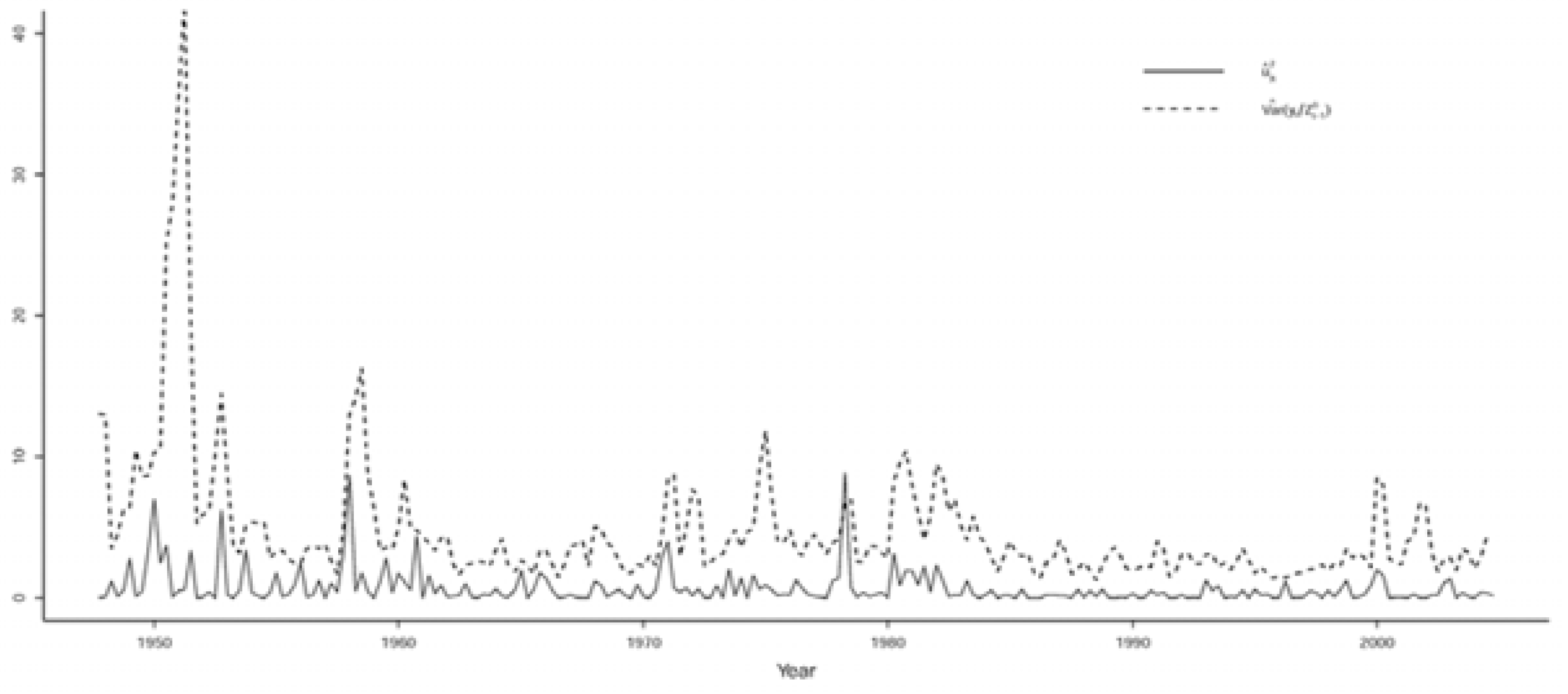
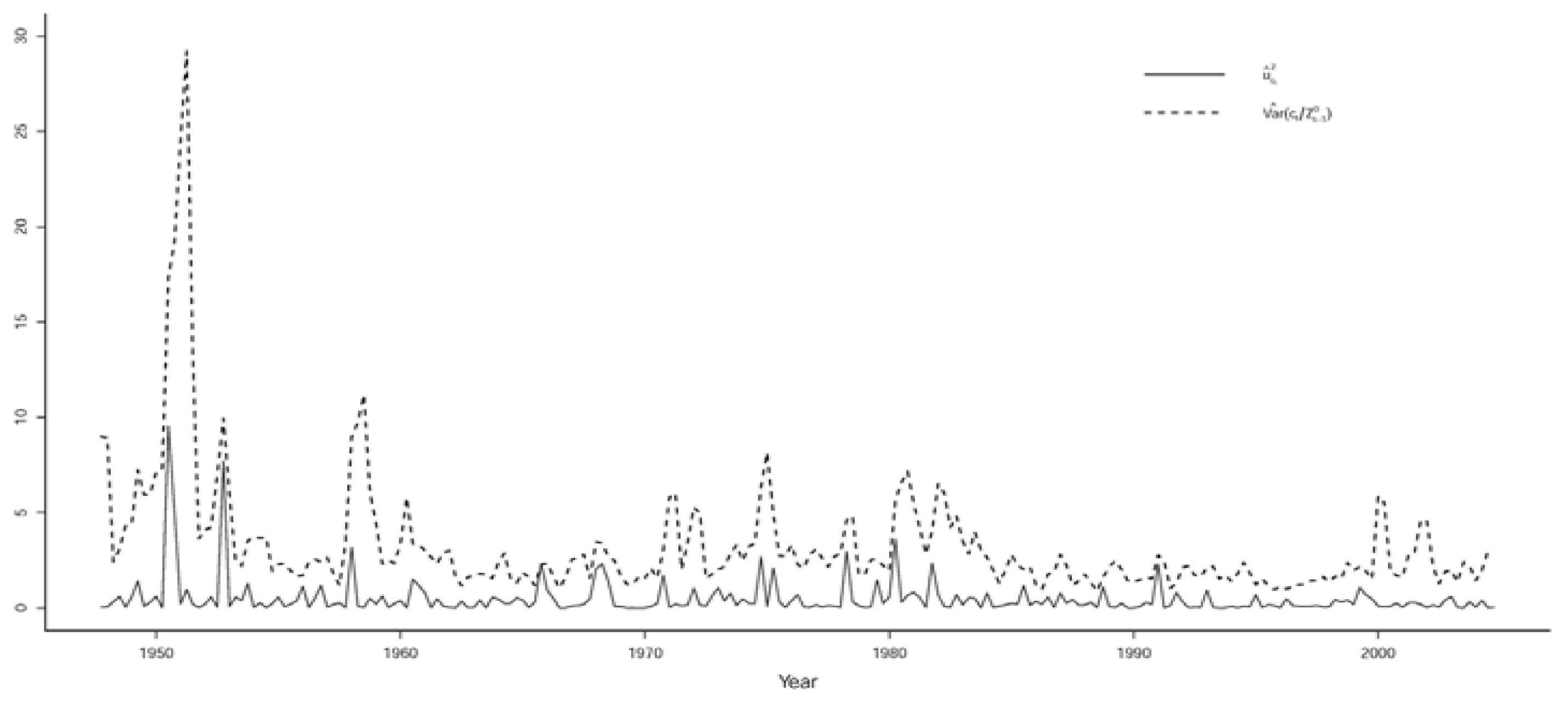
The inappropriateness of the constant conditional variance-covariance associated with the N-VAR(2) model is illustrated in Figure 1 and Figure 2, where the squared residuals from N-VAR(2) that exhibit great volatility are plotted with $\widehat{Var}\left(y_t\right|{\mathit{Z}}_{t-1}^0)$ and $\widehat{Var}\left(c_t\right|{\mathit{Z}}_{t-1}^0)$ based on the St-VAR(2) model (

Table 11. The estimated St-VAR(2) conditional variance St-VAR $\widehat{Var}\left(c_t\right|{\mathit{Z}}_{t-1}^0)$.

$\begin{array}{c}=\underset{\left(0.000\right)}{0.105}+\underset{\left(0.000\right)}{0.104}{\tilde{c}}_{t-1}^2+\underset{\left(0.000\right)}{0.107}{\tilde{c}}_{t-2}^2+\underset{\left(0.000\right)}{0.011}{\tilde{ı}}_{t-1}^2+\underset{\left(0.000\right)}{0.011}{\tilde{ı}}_{t-2}^2+\underset{\left(0.000\right)}{0.092}{\tilde{y}}_{t-1}^2+\underset{\left(0.000\right)}{0.080}{\tilde{y}}_{t-2}^2+\underset{\left(0.000\right)}{0.138}{\tilde{l}}_{t-1}^2+\underset{\left(0.000\right)}{0.140}{\tilde{l}}_{t-2}^2\hfill \\ +\underset{\left(0.000\right)}{0.271}{\tilde{\pi }}_{t-1}^2+\underset{\left(0.000\right)}{0.287}{\tilde{\pi }}_{t-2}^2+\underset{\left(0.000\right)}{0.100}{\tilde{w}}_{t-1}^2+\underset{\left(0.000\right)}{0.082}{\tilde{w}}_{t-2}^2+\underset{\left(0.000\right)}{2.393}{\tilde{r}}_{t-1}^2+\underset{\left(0.000\right)}{2.160}{\tilde{r}}_{t-2}^2-\underset{\left(0.007\right)}{0.004}{\tilde{c}}_{t-1}{\tilde{ı}}_{t-1}-\underset{\left(0.508\right)}{0.023}{\tilde{\pi }}_{t-2}{\tilde{r}}_{t-2}\hfill \\ -\underset{\left(0.000\right)}{0.041}{\tilde{c}}_{t-1}{\tilde{y}}_{t-1}-\underset{\left(0.258\right)}{0.007}{\tilde{c}}_{t-1}{\tilde{l}}_{t-1}+\underset{\left(0.013\right)}{0.020}{\tilde{c}}_{t-1}{\tilde{\pi }}_{t-1}-\underset{\left(0.022\right)}{0.010}{\tilde{c}}_{t-1}{\tilde{w}}_{t-1}-\underset{\left(0.235\right)}{0.025}{\tilde{c}}_{t-1}{\tilde{r}}_{t-1}+\underset{\left(0.000\right)}{0.033}{\tilde{c}}_{t-1}{\tilde{c}}_{t-2}\hfill \\ +\underset{\left(0.022\right)}{0.004}{\tilde{c}}_{t-1}{\tilde{ı}}_{t-2}-\underset{\left(0.000\right)}{0.018}{\tilde{c}}_{t-1}{\tilde{y}}_{t-2}+\underset{\left(0.081\right)}{0.011}{\tilde{c}}_{t-1}{\tilde{l}}_{t-2}+\underset{\left(0.066\right)}{0.015}{\tilde{c}}_{t-1}{\tilde{\pi }}_{t-2}-\underset{\left(0.983\right)}{0.000}{\tilde{c}}_{t-1}{\tilde{w}}_{t-2}+\underset{\left(0.600\right)}{0.014}{\tilde{c}}_{t-1}{\tilde{r}}_{t-2}\hfill \\ -\underset{\left(0.000\right)}{0.009}{\tilde{ı}}_{t-1}{\tilde{y}}_{t-1}-\underset{\left(0.001\right)}{0.007}{\tilde{ı}}_{t-1}{\tilde{l}}_{t-1}+\underset{\left(0.710\right)}{0.001}{\tilde{ı}}_{t-1}{\tilde{\pi }}_{t-1}-\underset{\left(0.071\right)}{0.003}{\tilde{ı}}_{t-1}{\tilde{w}}_{t-1}-\underset{\left(0.015\right)}{0.016}{\tilde{ı}}_{t-1}{\tilde{r}}_{t-1}+\underset{\left(0.199\right)}{0.002}{\tilde{ı}}_{t-1}{\tilde{c}}_{t-2}\hfill \\ -\underset{\left(0.000\right)}{0.002}{\tilde{ı}}_{t-1}{\tilde{ı}}_{t-2}-\underset{\left(0.722\right)}{0.001}{\tilde{ı}}_{t-1}{\tilde{y}}_{t-2}+\underset{\left(0.000\right)}{0.007}{\tilde{ı}}_{t-1}{\tilde{l}}_{t-2}+\underset{\left(0.697\right)}{0.001}{\tilde{ı}}_{t-1}{\tilde{\pi }}_{t-2}-\underset{\left(0.031\right)}{0.003}{\tilde{ı}}_{t-1}{\tilde{w}}_{t-2}+\underset{\left(0.314\right)}{0.007}{\tilde{ı}}_{t-1}{\tilde{r}}_{t-2}\hfill \\ -\underset{\left(0.000\right)}{0.041}{\tilde{y}}_{t-1}{\tilde{l}}_{t-1}+\underset{\left(0.122\right)}{0.011}{\tilde{y}}_{t-1}{\tilde{\pi }}_{t-1}-\underset{\left(0.000\right)}{0.019}{\tilde{y}}_{t-1}{\tilde{w}}_{t-1}-\underset{\left(0.247\right)}{0.024}{\tilde{y}}_{t-1}{\tilde{r}}_{t-1}-\underset{\left(0.001\right)}{0.020}{\tilde{y}}_{t-1}{\tilde{c}}_{t-2}-\underset{\left(0.001\right)}{0.017}{\tilde{y}}_{t-1}{\tilde{c}}_{t-2}\hfill \\ -\underset{\left(0.051\right)}{0.003}{\tilde{y}}_{t-1}{\tilde{ı}}_{t-2}+\underset{\left(0.000\right)}{0.020}{\tilde{y}}_{t-1}{\tilde{y}}_{t-2}+\underset{\left(0.000\right)}{0.040}{\tilde{y}}_{t-1}{\tilde{l}}_{t-2}-\underset{\left(0.148\right)}{0.012}{\tilde{y}}_{t-1}{\tilde{\pi }}_{t-2}+\underset{\left(0.309\right)}{0.022}{\tilde{y}}_{t-1}{\tilde{r}}_{t-2}-\underset{\left(0.874\right)}{0.001}{\tilde{l}}_{t-1}{\tilde{\pi }}_{t-1}\hfill \\ +\underset{\left(0.000\right)}{0.045}{\tilde{l}}_{t-1}{\tilde{w}}_{t-1}-\underset{\left(0.000\right)}{0.111}{\tilde{l}}_{t-1}{\tilde{r}}_{t-1}-\underset{\left(0.012\right)}{0.016}{\tilde{l}}_{t-1}{\tilde{c}}_{t-2}+\underset{\left(0.494\right)}{0.003}{\tilde{y}}_{t-1}{\tilde{w}}_{t-2}-\underset{\left(0.110\right)}{0.003}{\tilde{l}}_{t-1}{\tilde{ı}}_{t-2}-\underset{\left(0.003\right)}{0.016}{\tilde{l}}_{t-1}{\tilde{y}}_{t-2}\hfill \\ -\underset{\left(0.000\right)}{0.136}{\tilde{l}}_{t-1}{\tilde{l}}_{t-2}-\underset{\left(0.630\right)}{0.005}{\tilde{l}}_{t-1}{\tilde{\pi }}_{t-2}+\underset{\left(0.208\right)}{0.008}{\tilde{l}}_{t-1}{\tilde{w}}_{t-2}-\underset{\left(0.609\right)}{0.014}{\tilde{l}}_{t-1}{\tilde{r}}_{t-2}+\underset{\left(0.000\right)}{0.041}{\tilde{\pi }}_{t-1}{\tilde{w}}_{t-1}-\underset{\left(0.469\right)}{0.026}{\tilde{\pi }}_{t-1}{\tilde{r}}_{t-1}\hfill \\ -\underset{\left(0.022\right)}{0.019}{\tilde{\pi }}_{t-1}{\tilde{c}}_{t-2}-\underset{\left(0.999\right)}{0.000}{\tilde{\pi }}_{t-1}{\tilde{ı}}_{t-2}+\underset{\left(0.957\right)}{0.000}{\tilde{\pi }}_{t-1}{\tilde{y}}_{t-2}+\underset{\left(0.433\right)}{0.007}{\tilde{\pi }}_{t-1}{\tilde{l}}_{t-2}-\underset{\left(0.000\right)}{0.208}{\tilde{\pi }}_{t-1}{\tilde{\pi }}_{t-2}-\underset{\left(0.001\right)}{0.026}{\tilde{\pi }}_{t-1}{\tilde{w}}_{t-2}\hfill \\ -\underset{\left(0.033\right)}{0.078}{\tilde{\pi }}_{t-1}{\tilde{r}}_{t-2}+\underset{\left(0.415\right)}{0.017}{\tilde{w}}_{t-1}{\tilde{r}}_{t-1}-\underset{\left(0.033\right)}{0.011}{\tilde{w}}_{t-1}{\tilde{c}}_{t-2}+\underset{\left(0.545\right)}{0.001}{\tilde{w}}_{t-1}{\tilde{ı}}_{t-2}-\underset{\left(0.108\right)}{0.007}{\tilde{w}}_{t-1}{\tilde{y}}_{t-2}-\underset{\left(0.000\right)}{0.054}{\tilde{\pi }}_{t-1}{\tilde{l}}_{t-2}\hfill \\ -\underset{\left(0.000\right)}{0.042}{\tilde{w}}_{t-1}{\tilde{\pi }}_{t-2}-\underset{\left(0.644\right)}{0.002}{\tilde{w}}_{t-1}{\tilde{w}}_{t-2}+\underset{\left(0.353\right)}{0.021}{\tilde{w}}_{t-1}{\tilde{r}}_{t-2}-\underset{\left(0.283\right)}{0.026}{\tilde{r}}_{t-1}{\tilde{c}}_{t-2}-\underset{\left(0.006\right)}{0.022}{\tilde{r}}_{t-1}{\tilde{ı}}_{t-2}-\underset{\left(0.591\right)}{0.011}{\tilde{r}}_{t-1}{\tilde{y}}_{t-2}\hfill \\ +\underset{\left(0.003\right)}{0.089}{\tilde{r}}_{t-1}{\tilde{l}}_{t-2}-\underset{\left(0.009\right)}{0.106}{\tilde{r}}_{t-1}{\tilde{\pi }}_{t-2}-\underset{\left(0.523\right)}{0.014}{\tilde{r}}_{t-1}{\tilde{w}}_{t-2}-\underset{\left(0.000\right)}{0.511}{\tilde{r}}_{t-1}{\tilde{r}}_{t-2}-\underset{\left(0.046\right)}{0.003}{\tilde{c}}_{t-2}{\tilde{ı}}_{t-2}-\underset{\left(0.000\right)}{0.041}{\tilde{c}}_{t-2}{\tilde{y}}_{t-2}\hfill \\ +\underset{\left(0.003\right)}{0.019}{\tilde{c}}_{t-2}{\tilde{l}}_{t-2}+\underset{\left(0.000\right)}{0.051}{\tilde{c}}_{t-2}{\tilde{\pi }}_{t-2}-\underset{\left(0.220\right)}{0.005}{\tilde{c}}_{t-2}{\tilde{w}}_{t-2}+\underset{\left(0.641\right)}{0.009}{\tilde{c}}_{t-2}{\tilde{r}}_{t-2}-\underset{\left(0.000\right)}{0.012}{\tilde{ı}}_{t-2}{\tilde{y}}_{t-2}-\underset{\left(0.216\right)}{0.002}{\tilde{ı}}_{t-2}{\tilde{l}}_{t-2}\hfill \\ +\underset{\left(0.216\right)}{0.003}{\tilde{ı}}_{t-2}{\tilde{\pi }}_{t-2}+\underset{\left(0.446\right)}{0.001}{\tilde{ı}}_{t-2}{\tilde{w}}_{t-2}-\underset{\left(0.000\right)}{0.028}{\tilde{ı}}_{t-2}{\tilde{r}}_{t-2}+\underset{\left(0.005\right)}{0.017}{\tilde{y}}_{t-2}{\tilde{l}}_{t-2}-\underset{\left(0.860\right)}{0.001}{\tilde{y}}_{t-2}{\tilde{\pi }}_{t-2}-\underset{\left(0.028\right)}{0.008}{\tilde{y}}_{t-2}{\tilde{w}}_{t-2}\hfill \\ -\underset{\left(0.006\right)}{0.049}{\tilde{y}}_{t-2}{\tilde{r}}_{t-2}+\underset{\left(0.205\right)}{0.012}{\tilde{l}}_{t-2}{\tilde{\pi }}_{t-2}-\underset{\left(0.145\right)}{0.008}{\tilde{l}}_{t-2}{\tilde{w}}_{t-2}-\underset{\left(0.647\right)}{0.012}{\tilde{l}}_{t-2}{\tilde{r}}_{t-2}+\underset{\left(0.000\right)}{0.036}{\tilde{\pi }}_{t-2}{\tilde{w}}_{t-2}+\underset{\left(0.006\right)}{0.048}{\tilde{w}}_{t-2}{\tilde{r}}_{t-2}\hfill \end{array}$

), indicating that they capture most of the volatility. Note that all seven conditional variances are scaled versions of each other.

3.3.3. Evaluating the Statistical Adequacy of the St-VAR(2) Model

To take into account the heteroskedastic conditional variance-covariance, one needs to reconsider the notion of what constitutes the ‘relevant residuals’ for M-S testing purposes. In the case of the St-VAR(p) model the relevant residuals are the standardized ones defined by:

$$\begin{array}{c}{\widehat{\mathit{u}}}_t={\mathit{L}}_t^{-1}({\mathit{Z}}_t-{\widehat{\mathit{Z}}}_t)\end{array}$$

(8)

where ${\mathit{L}}_t{\mathit{L}}_t^{\top }=\widehat{Var}({\mathit{Z}}_t{\left|\sigma \right(\mathit{Z}}_{t-1}^0\left)\right)$, ${\widehat{\mathit{Z}}}_t={\widehat{\mathit{\delta }}}_0+{\widehat{\mathit{\delta }}}_{1}t+{\widehat{\mathit{A}}}_1^{\top }{\mathit{Z}}_{t-1}+{\widehat{\mathit{A}}}_2^{\top }{\mathit{Z}}_{t-2}.$ Here, ${\mathit{L}}_t$ is changing with t and ${\mathit{Z}}_{t-1}^0$ as opposed to being constant in the N-VAR(2) model. An indicative pair of auxiliary regressions based on these residuals is:

$$\begin{array}{c}{\widehat{u}}_t=a_0+a_1{\widehat{y}}_t+b_3{\widehat{y}}_t^2+b_1{\widehat{u}}_{t-1}+b_2{\widehat{u}}_{t-2}+b_4{t}^2+b_5{t}^3+v_{1t},\\ {\widehat{u}}_t^2={\gamma }_0+{\gamma }_1{\widehat{\sigma }}_t^2+c_1{\widehat{y}}_t^2+c_2{\widehat{\sigma }}_{t-1}^2+c_3{\widehat{\sigma }}_{t-2}^2+c_{4}t+c_5{t}^2+v_{2t},\end{array}$$

where ${\widehat{y}}_t$ denotes the fitted values and ${\widehat{\sigma }}_t^2$ = $\widehat{Var}\left(y_t\right|\sigma \left({\mathit{Z}}_{t-1}^0\right))$. The hypotheses being tested are directly analogous to those in Table 5 above.

The results of the M-S testing for the estimated Student’s VAR(2) model, reported in

Table 12. M-S Testing results for St-VAR(2).

	$\begin{array}{c}{\mathit{c}}_{\mathit{t}}\end{array}$	$\begin{array}{c}{\mathit{i}}_{\mathit{t}}\end{array}$	$\begin{array}{c}{\mathit{y}}_{\mathit{t}}\end{array}$	$\begin{array}{c}{\mathit{l}}_{\mathit{t}}\end{array}$	$\begin{array}{c}{\mathit{\pi }}_{\mathit{t}}\end{array}$	$\begin{array}{c}{\mathit{w}}_{\mathit{t}}\end{array}$	$\begin{array}{c}{\mathit{z}}_{\mathit{t}}\end{array}$
[2] Linearity	1.598[0.208]	2.312[0.130]	0.844[0.359]	0.003[0.957]	1.244[0.266]	0.000[0.986]	6.337[0.013]
[4] 1st depend	0.316[0.575]	0.249[0.619]	0.610[0.436]	1.888[0.171]	0.627[0.429]	0.146[0.703]	0.905[0.342]
[5] 1st-invar	0.697[0.499]	1.157[0.316]	1.398[0.249]	0.972[0.380]	1.548[0.215]	1.268[0.284]	0.206[0.814]
[3] Heterosked	0.009[0.925]	0.250[0.617]	1.320[0.252]	0.009[0.926]	3.085[0.080]	0.009[0.924]	0.075[0.785]
[4] 2nd depend	0.199[0.820]	0.748[0.475]	0.666[0.515]	0.384[0.682]	1.308[0.273]	0.447[0.640]	0.303[0.739]
[5] 2nd t-invar	0.388[0.679]	0.153[0.858]	0.537[0.585]	0.010[0.990]	1.706[0.184]	3.339[0.037]	5.142[0.010]
[1] A-D test	0.763[0.508]	0.961[0.378]	0.823[0.465]	0.841[0.452]	1.666[0.141]	1.130[0.296]	1.790[0.120]

, indicate no departures from its assumptions [1]–[5]. In assessing these results it is important to note that the p-values decrease with the sample size n, implying that one needs to decrease the appropriate threshold as n increases. For $n=231,$ a more appropriate threshold is $\alpha =0.01$; see (Spanos 2014).

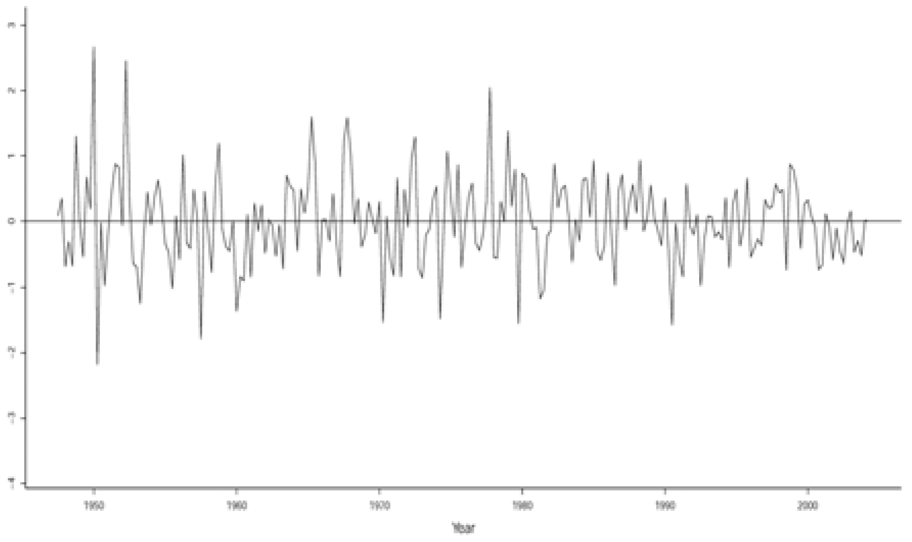
The statistical adequacy of the St-VAR(2) is also reflected by the constancy of the variation around a constant mean, exhibited by its residuals in Figure 3.

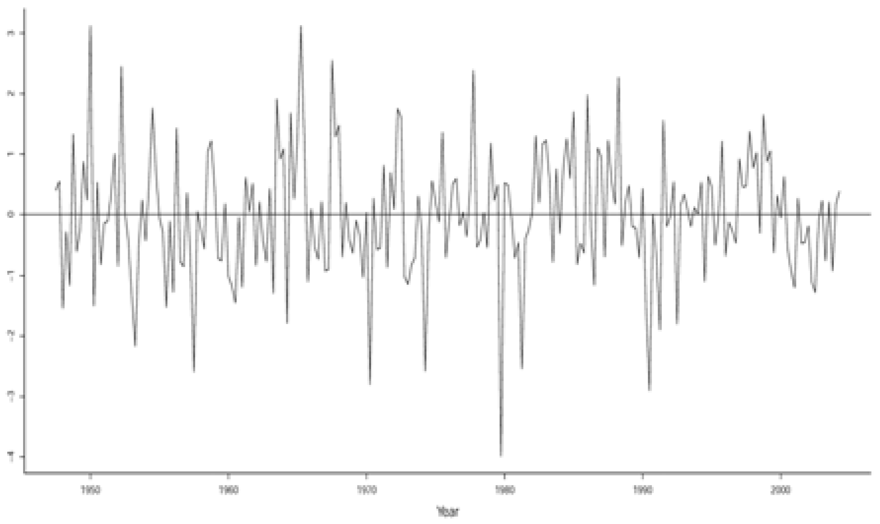
This should be contrasted with the N-VAR(2) residuals in Figure 4 which seem to indicate a shift in both the mean and variance between the period 1983–2000 and afterward. This, however, is misleading since Figure 4 represents the residuals of a statistically misspecified model. On the other hand, Figure 3 represents the residuals of a statistically adequate model and suggests that the lower volatility arises as an inherent chance regularity stemming from $\{{\mathit{Z}}_t,t\in \mathbb{N}\}$ being a Student’s t Markov (2) process. Indeed, the sequence of successive periods of large and small volatility represents a chance regularity pattern reflecting second-order temporal dependence, initially noted by (Mandelbrot 1963):

“...large changes tend to be followed by large changes-of either sign-and small changes tend to be followed by small changes”.

(p. 418)

This calls into question the hypothesis known as the ‘great moderation’ (Stock and Watson 2002) based on Figure 4, since the residuals from the N-VAR(2) model do not account for the second-order dependence. That is, the ‘great moderation’ hypothesis stems form an erroneous interpretation based on statistical misspecification. The relevant residuals from a statistically adequate St-VAR(2) model in Figure 3 represent a realization of a Student’s t Martingale Difference process as they should.

4. Evaluating the Smets and Wouters DSGE Model

4.1. Testing the Over-Identifying Restrictions

In light of the fact that the Student’s t VAR(2) is a statistically adequate model, one can proceed to probe the empirical adequacy of the DSGE model, knowing that the actual error probabilities provide a close approximation to the nominal (assumed) ones. This includes testing the DSGE over-identifying restrictions:

$$\begin{array}{c}{H}_0\text{:}\mathit{G}\left(\mathit{\theta },\mathit{\phi }\right)=0,\mathrm{vs}.H_1\text{:}\mathit{G}\left(\mathit{\theta },\mathit{\phi }\right)\ne 0,\mathrm{for}\mathit{\theta }\in \Theta ,\mathit{\phi }\in \Phi ,\end{array}$$

The relevant test is based on the likelihood ratio statistic:

$$\begin{array}{c}{\lambda }_n\left(\mathit{Z}\right)=\frac{{max}_{\mathit{\phi }\in \Phi }L(\mathit{\phi };\mathit{Z})}{{max}_{\mathit{\theta }\in \Theta }L(\mathit{\theta };\mathit{Z})}=\frac{L(\tilde{\mathit{\phi }};\mathit{Z})}{L(\widehat{\mathit{\theta }};\mathit{Z})}\Rightarrow -2ln{\lambda }_n\left(\mathit{Z}\right)\stackrel{H_0}{\underset{a}{\backsim }}{\chi }^2\left(m\right).\end{array}$$

(9)

For $m=98$, for $\alpha =0.01,c_{\alpha }=68.4,$ the observed test statistic yields:

$$\begin{array}{c}-2ln{\lambda }_n\left({\mathit{Z}}_0\right)>50165.3\left[0.00000000\right].\end{array}$$

The tiny p-value provides indisputably strong evidence against the DSGE model.

Hence, when a DSGE model ${\mathcal{M}}_{\mathit{\phi }}\left(\mathit{z}\right)$ is tested against reliable statistical evidence in the form of a statistically adequate ${\mathcal{M}}_{\mathit{\theta }}\left(\mathit{z}\right)$ [Student’s t VAR(2)], ${\mathcal{M}}_{\mathit{\phi }}\left(\mathit{z}\right)$ is strongly rejected. The natural way forward for DSGE modeling is to find ways to modify DSGE models with a view to account for the statistical regularities in the data brought out by the Student’s t VAR(2). These regularities include the leptokurticity as well as the second-order temporal dependence exemplified by the heteroskedastic $Var\left({\mathit{Y}}_t\right|{\mathit{Z}}_{t-1}^0).$

It is important to note that the (Del Negro et al. 2007) substantive misspecification analysis based on the DSGE-VAR($\lambda$) model differs from the above frequentist over-identifying restrictions test; see (Consolo et al. 2009). Apart from the fact that the former uses a Bayesian approach, the key difference is that the probabilistic assumptions underlying the VAR($\lambda$) specification are presumed valid and are not tested against the data.

4.2. Forecasting Performance

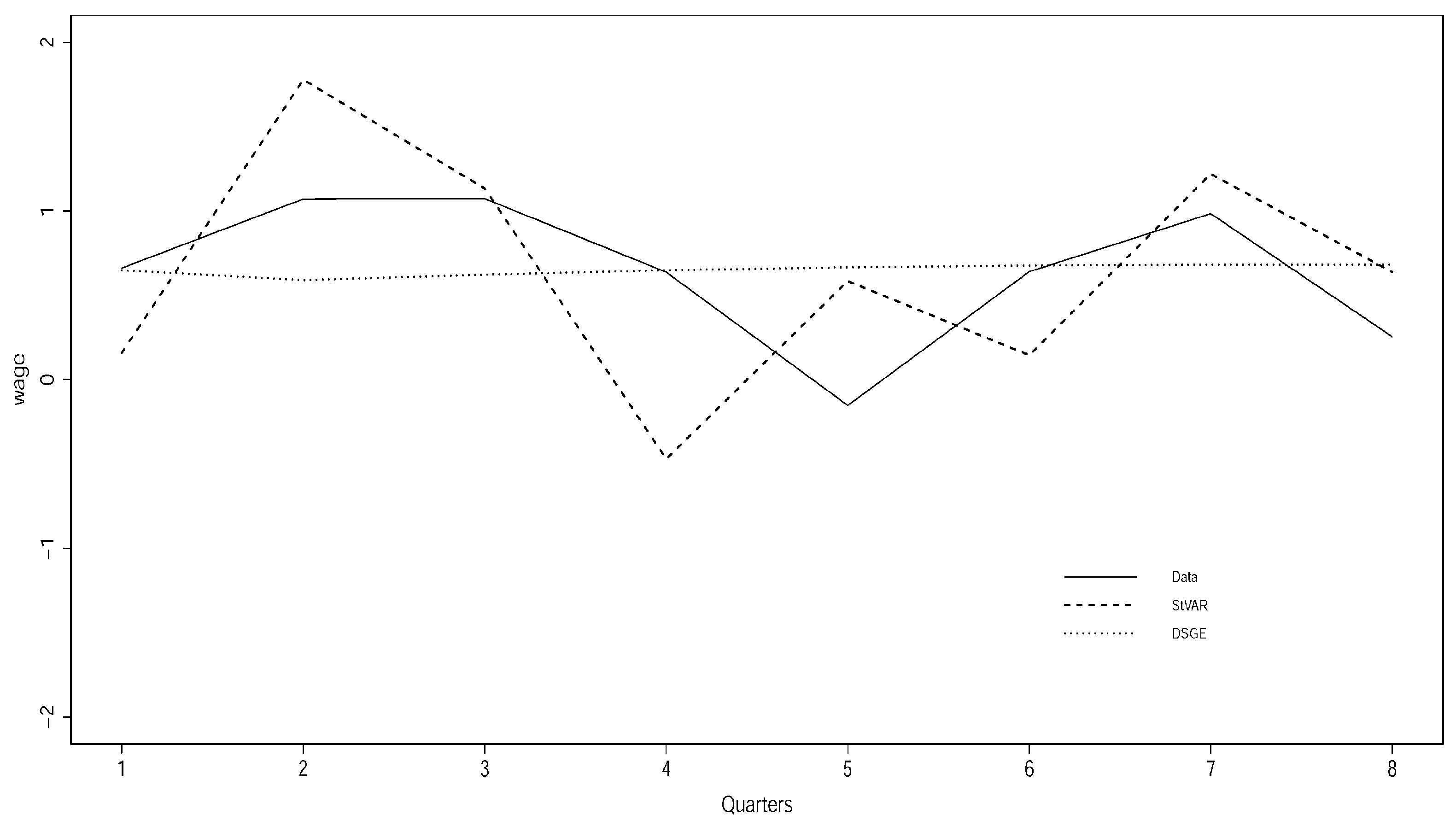
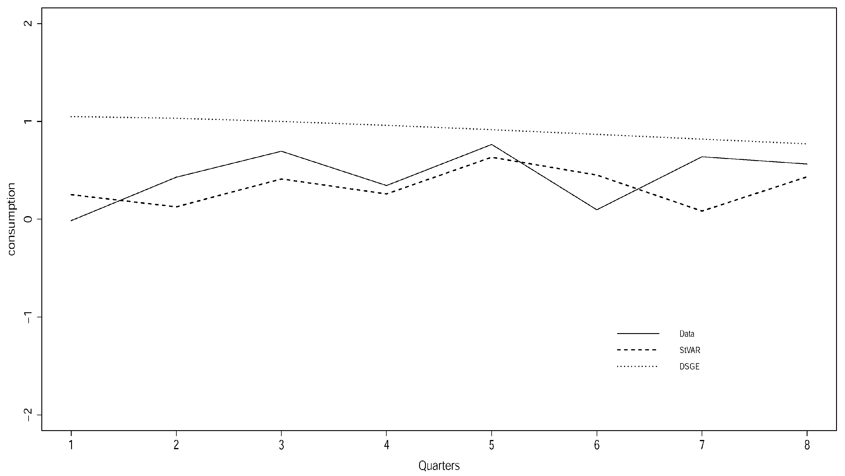
Typical examples of out-of-sample forecasting capacity of both the DSGE and the Student’s t VAR(2) models for 8 periods ahead [2003Q1-2004Q4; estimation period 1947Q2-2002Q4] is shown in Figure 5 and Figure 6 for wages and consumption growth, with the actual data denoted by a solid line.

Figure 5 and Figure 6 are typical cases of the forecasting performance of the Smets and Wouters DSGE model and illustrate a good and a bad case. In general, the forecast line of the DSGE model tends to be over smoothed in a way that largely ignores the systematic temporal dependence/heterogeneity in the data. When the forecast line happens to overlap with the actual data, it appears to track the trend reasonably well but not the cycles; see Figure 6.

When the forecast line misses the actual data line (see Figure 6), the forecasts are particularly bad because the DSGE model over or under predicts systematically, giving rise to systematic (non-white noise) prediction errors. This pattern is symptomatic of statistical msisspecification. In relation to this, it is very important to emphasize that when the forecasts errors are statistically systematic—they exhibit over or under prediction—the Root Mean Square Error (RMSE) can be highly misleading as a measure of forecasting capacity. The RMSE is a reliable measure only when the forecast errors are statistically non-systematic. In that sense, Figure 5 and Figure 6 show that the performance of the St-VAR(2) model is much better than that of the DSGE model, irrespective of the RMSEs.

Note that in the case of the St-VAR model, statistically non-systematic means that its residuals and forecast errors constitute realizations of martingale difference processes.

Interestingly, the poor forecasting performance of DSGE models is well-known, but it is rendered acceptable by comparing it to that of N-VAR models:

“...we find that the benchmark estimated medium scale DSGE model forecasts inflation and GDP growth very poorly, although statistical and judgemental forecasts do equally poorly”.

(Edge and Gurkaynak 2010, p. 209)

This claim fails to recognize that the poor forecasting performance stems primarily from the statistical inadequacy of the underlying estimated model; see Table 6 and Table 7.

4.3. Potentially Misleading Impulse Response Analysis

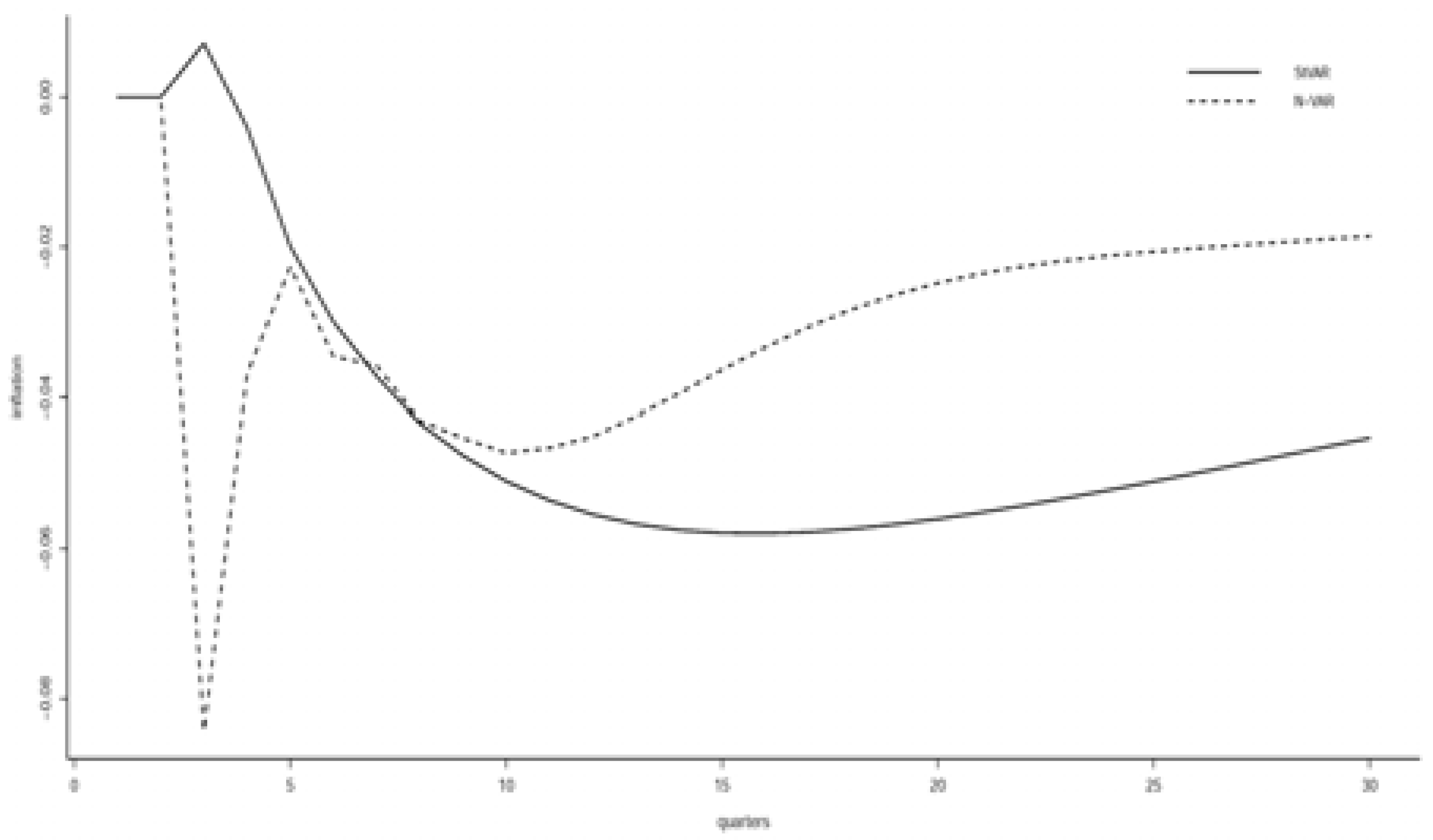
The statistical inadequacy of the underlying statistical model also affects the reliability of its impulse response analysis, giving rise to misleading results about the reaction to exogenous shocks over time. Indeed, the estimated $\widehat{Var}\left(y_t\right|{\mathit{Z}}_{t-1}^0)$ brings out the potential unreliability of any impulse response and variance decomposition analysis based on assuming a constant conditional variance.

Figure 7 compares the impulse responses of a $1\%$ increase in labor hours ($l_t$) on inflation (${\pi }_t$) from the Normal and Student’s t VAR models. The statistically adequate St-VAR(2) model produces a sharp and big decline and a slow recovery in the rate of inflation. However, the Normal VAR model produces a different impulse response. The rate of inflation decreases sharply first, and then sharply increases before falling again and rising slowly.

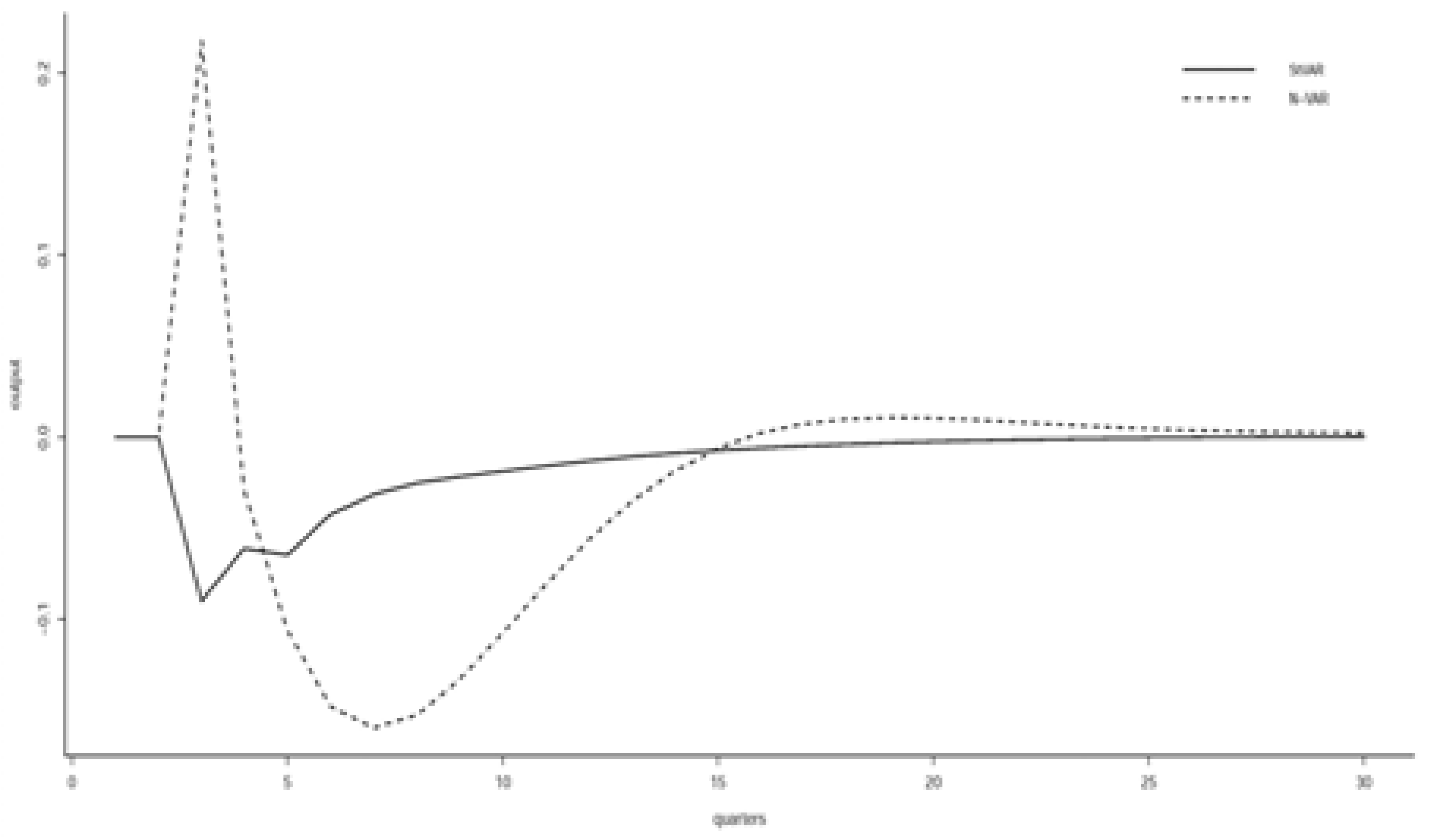
Figure 8 compares the impulse responses of a $1\%$ increase in labor hours rate ($l_t$) on output ($y_t$) from the Normal and Student’s t VAR models. The heterogeneous St-VAR model produces a mild decline and a slow recovery in the growth rate of per-capita real GDP. But the effects produced by the stationary Normal VAR model are completely different. The growth rate increases first, falls and recovers slowly.

4.4. Identification of the ‘Deep’ Structural Parameters

A crucial issue raised in the DSGE literature is the identification of the structural parameters; see (Canova 2007; Iskrev 2010). The problem is that there is often no direct way to relate the statistical parameters ($\mathit{\theta }$) to the structural parameters ($\mathit{\phi }$) because the implicit function $\mathit{G}(\mathit{\theta },\mathit{\phi })=\mathbf{0}$ is not only highly non-linear, but it also involves algorithms like the Schur decomposition of the structural matrices involved.

An indirect way to probe the identification of the above DSGE model is to use the estimated statistical model, St-VAR(2) to generate, say N, faithful (true to the probabilistic structure of ${\mathit{Z}}_0$)replications of the original data ${\mathit{Z}}_0$. The statistical adequacy of the estimated St-VAR(2) ensures that it accounts for the statistical regularities in the data, and thus the simulated data will have the same probabilistic structure as the original observations. This enables the modeler to learn about the identifiability of the deep parameters using these faithful replicas of the original data to estimate the structural DSGE model.

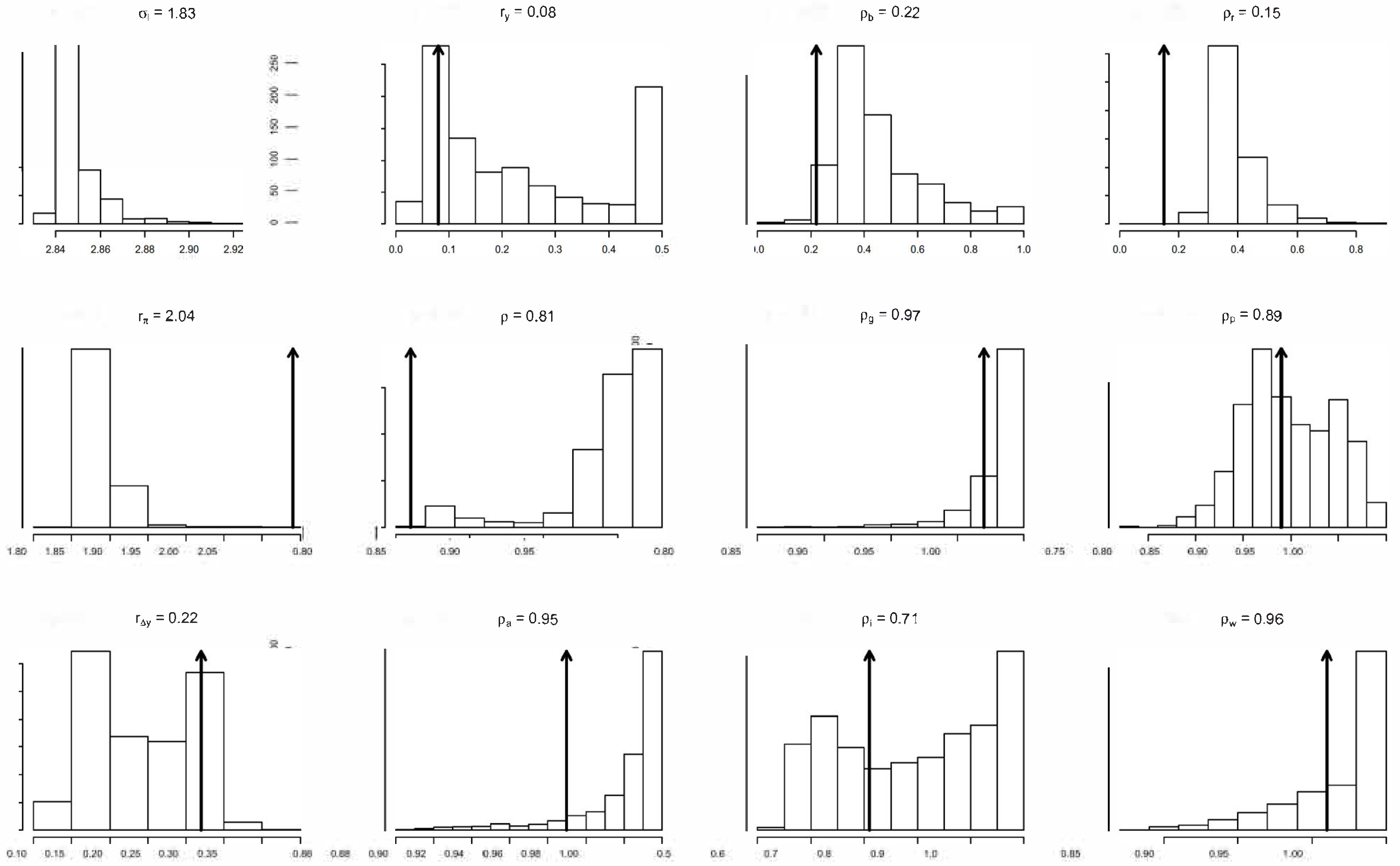
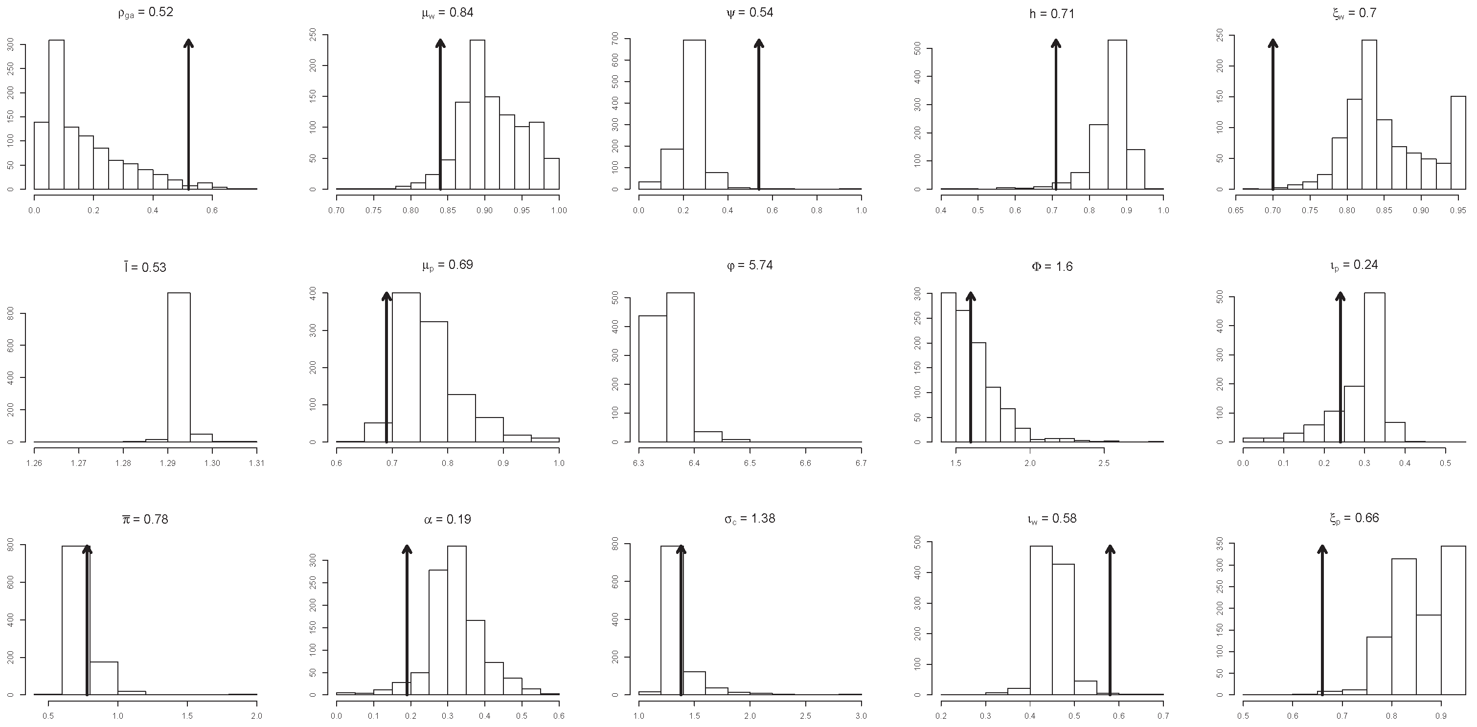
The N simulated data series can be used to estimate the structural parameters ($\mathit{\phi }$) using the original ‘quantification’ procedures in (Smets and Wouters 2007). When the histogram of each ${\widehat{\mathit{\phi }}}_i,$ for $i=1,2,\dots ,p,$ is concentrated around a particular value, with a narrow interval of support, then ${\mathit{\phi }}_i$ can be regarded as identifiable. When the histogram exhibits a large range of values or/and multiple modes, it indicates that the parameter in question is non-identifiable.

Out of 36 parameters, simulation is applied to 27 keeping the rest of the parameters (7 of them are the variance of the shocks) constant. The 27 histograms in Figure 9 and Figure 10 were generated using $N=3000$ replications of the original data of sample size $n=230$ based on the estimated statistical model, St-VAR(2); increasing N does not change the above results. Looking at these histograms we can distinguish between three different groups of identified/non-identified parameters.

First is the group where the estimated/calibrated value is close to the mode of the histogram. In this case, the parameters $\left(\overline{\pi },{\mu }_p,{\sigma }_c,\Phi ,{\rho }_p,{\rho }_g\right)$ are potentially identifiable vis-a-vis the data.

Second is the group where the estimated/calibrated values are significantly different from the mode of the histogram. In such a case, the parameters in question $\left(\overline{l},\alpha ,\mathit{\phi },h,{\iota }_w,{\iota }_p,{\sigma }_l,r_{\pi },\rho ,{\rho }_a,{\rho }_r,{\rho }_w\right)$ are likely to be unidentifiable.

Third is the group where the estimated/calibrated value lies outside the actual range of values of the histogram. The parameters in question $\left({\rho }_{ga},{\mu }_w,{\xi }_w,{\xi }_p,r_y,{\rho }_i,{\rho }_b,{\rho }_p\right)$ are clearly non-identifiable.

Taken together, only six of the twenty-seven parameters have estimated or calibrated values that are potentially identifiable vis-a-vis the data.

This simulation exercise indicates that, in contrast to the statistical parameters of the St-VAR(2) which are inherently identifiable, the identification and constancy of the ‘deep’ DSGE parameters is called into question. The results also question the appropriateness of the ‘estimation’ of these deep parameters using traditional methods such as the method of moments, maximum likelihood, and Bayesian techniques; see (Smets and Wouters 2003, 2005, 2007; Ireland 2004, 2011). A question that needs to be addressed is whether the Bayesian techniques narrow down the range of values of the deep parameters to render them “artificially” identifiable. Indeed, the broader question which naturally arises when one is dealing with a calibrated model is: what is one calibrating/evaluating when the structural parameters are non-identifiable?

4.5. Substantive vs. Statistical Adequacy

Lucas’s (Lucas 1980) argument that: “Any model that is well enough articulated to give clear answers to the questions we put to it will necessarily be artificial, abstract, patently ‘unreal’” (p. 696), is highly misleading because it blurs the distinction between substantive and statistical adequacy. There is nothing wrong with constructing a simple, abstract, and idealized theory-model ${\mathcal{M}}_{\mathit{\phi }}\left(\mathit{z}\right)$ aiming to capture key features of the phenomenon of interest, to shed light on (understand, explain, forecast) economic phenomena of interest, as well as gain insight concerning alternative policies. Unreliability of inference problems arise when the statistical model ${\mathcal{M}}_{\mathit{\theta }}\left(\mathit{z}\right)$ implicitly specified by ${\mathcal{M}}_{\mathit{\phi }}\left(\mathit{z}\right)$ is statistically misspecified, and no attempt is made to reliably assess whether ${\mathcal{M}}_{\mathit{\phi }}\left(\mathit{z}\right)$ does, indeed, capture the key features of the phenomenon of interest; see (Spanos 2009a). That is, the strategy ‘theory or bust’ makes no sense in empirical modeling. As argued by Hendry (Hendry 2009):

“This implication is not a tract for mindless modeling of data in the absence of economic analysis, but instead suggests formulating more general initial models that embed the available economic theory as a special case, consistent with our knowledge of the institutional framework, historical record, and the data properties...Applied econometrics cannot be conducted without an economic theoretical framework to guide its endeavors and help interpret its findings. Nevertheless, since economic theory is not complete, correct, and immutable, and never will be, one also cannot justify an insistence on deriving empirical models from theory alone”.

(pp. 56–57)

Statistical misspecification is not the inevitable result of abstraction and simplification but stems from imposing invalid probabilistic assumptions on the data. Moreover, the latter goes a long way toward explaining the poor forecasting performance of the traditional macroeconometric models in the 1970s (Nelson 1972) and can explain the poor forecasting performance of DSGE models.

Unfortunately, the current literature on DSGE modeling adopts the (Kydland and Prescott 1991) view that misspecification is inevitable. For instance, (Canova 2007) goes further by arguing: “DSGE models are misspecified in the sense that they are, in general, too simple to capture the complex probabilistic nature of the data. Hence, it may be fruitless to compare their outcomes with the data...Both academic economists and policy makers use DSGE models to tell stories about how the economy responds to unexpected movements in the exogenous variables”. (p. 160)

There is nothing complicated about the probabilistic nature of economic time series data. The probabilistic assumptions needed to account for the chance regularity patterns in such data come from three broad categories, (D) Distribution, (M) Dependence, and (H) Heterogeneity, with simple generic ways to account for (M) and (H) using lags and trend polynomials. Moreover, when any of the probabilistic assumptions are found wanting, they can be easily replaced with more appropriate ones (respecification); see Spanos (2019). Regarding the use of empirical modeling as ‘story-telling’, it should noted that when an estimated DSGE model (${\mathcal{M}}_{\psi }\left(\mathit{z}\right))$ is statistically misspecified, then the stories based on it have nothing to do with the economy that gave rise to the data since the empirical evidence invoked are untrustworthy. It will be better for the scientific reputation of macroeconometrics to skip the ‘data’ part and just tell the stories associated with simulating ${\mathcal{M}}_{\psi }\left(\mathit{z}\right)$ using parameter values that seem ‘appropriate’ to a DSGE modeler. Why pretend that these values stem from the data?

5. Summary and Conclusions

The literature on DSGE modeling rightly points out that reliance on chance regularities for statistical inference purposes, as in the case of the traditional VAR(p) model, is not sufficient to represent substantively meaningful (structural) models that can be used to forecast and evaluate different macroeconomic policies. On the other hand, estimating structural models that belie the chance regularities in the data would only give rise to untrustworthy inference results.

Estimating the structural model directly often leads to an impasse since the estimated model is often both statistically and substantively inadequate. This renders any proposed substantive respecifications of the original structural model (Del Negro and Schorfeide 2009; Del Negro et al. 2007) questionable since the respecified model is declared ‘better’ or ‘worse’ on the basis of untrustworthy evidence when the estimated statistical model is misspecified.

A way to address this quandary is to separate, ab initio, the structural model ${\mathcal{M}}_{\mathit{\phi }}\left(\mathit{z}\right)$ from the statistical model ${\mathcal{M}}_{\mathit{\theta }}\left(\mathit{z}\right),$ and establish statistical adequacy before posing any substantive questions of interest. An estimated DSGE model ${\mathcal{M}}_{\mathit{\phi }}\left(\mathit{z}\right)$ whose statistical premises ${\mathcal{M}}_{\mathit{\theta }}\left(\mathit{z}\right)$ are misspecified constitutes an unreliable basis for any form of inference. From a purely probabilistic perspective, ${\mathcal{M}}_{\mathit{\theta }}\left(\mathit{z}\right)$ is viewed as a parameterization of the process $\{{\mathit{Z}}_t,t\in \mathbb{N}\}$ underlying data ${\mathit{Z}}_0,$ chosen so that it (parametrically) nests ${\mathcal{M}}_{\mathit{\phi }}\left(\mathit{z}\right)$ via $\mathit{G}\left(\mathit{\theta },\mathit{\phi }\right)=\mathbf{0}.$ The crucial distinction between statistical and substantive premises suggests that various traditional conundrums, such as theory-driven vs. data-driven, realistic vs. unrealistic, and policy-oriented vs. non-policy-oriented models, are largely false dilemmas. Statistical adequacy of ${\mathcal{M}}_{\mathit{\theta }}\left(\mathit{z}\right)$ is a necessary precondition for securing the reliability of any form of inference.

Using quarterly US data for the period 1947:2–2004:4, the confrontation of the (Smets and Wouters 2007) DSGE model ${\mathcal{M}}_{\mathit{\phi }}\left(\mathit{z}\right)$ with a statistically adequate ${\mathcal{M}}_{\mathit{\theta }}\left(\mathit{z}\right)$ [Student’s t VAR(2)] strongly rejects${\mathcal{M}}_{\mathit{\phi }}\left(\mathit{z}\right),$ and calls into question the reliability of any inferences based on it. The Bayesian estimation techniques used by the authors are likely to be equally unreliable because the implicit likelihood function is invalid. Indeed, in light of the unidentifiability of most of the structural parameters shown in Section 4.4, questions arise about the role of the priors in quantifying such parameters. Based on the above discussion, a way forward for DSGE modeling is to engage in the following recommendations.

(a)

The modeler needs to bring out the statistical model ${\mathcal{M}}_{\mathit{\theta }}\left(\mathit{z}\right)$ implicitly specified by the structural model ${\mathcal{M}}_{\mathit{\phi }}\left(\mathit{z}\right)$, with the former specified in terms of a complete set of testable probabilistic assumptions, as in Table 1, Table 4 and Table 8.

(b)

When a DSGE model ${\mathcal{M}}_{\mathit{\phi }}\left(\mathit{z}\right)$ is estimated directly, the statistical reliability of any inferences drawn is questionable. Before any reliable inferences can be drawn, the modeler needs to test the validity of the assumptions of the statistical model.

(c)

When the statistical model ${\mathcal{M}}_{\mathit{\theta }}\left(\mathit{z}\right)$ is found to be misspecified, the modeler needs to respecify it to account for the statistical information in the data. Only when the statistical adequacy of ${\mathcal{M}}_{\mathit{\theta }}\left(\mathit{z}\right)$ is established, one should proceed to the inference stage.

(d)

The evaluation of the empirical validity of the structural model ${\mathcal{M}}_{\mathit{\phi }}\left(\mathit{z}\right)$ begins with testing the validity of the over-identifying restrictions $\mathit{G}\left(\mathit{\theta },\mathit{\phi }\right)=\mathbf{0},$ in the context of a statistically adequate ${\mathcal{M}}_{\mathit{\theta }}\left(\mathit{z}\right)$.

(e)

In cases where the overidentifying restrictions are rejected, the modeler needs to return to ${\mathcal{M}}_{\mathit{\phi }}\left(\mathit{z}\right)$ in order to respecify it substantively, to account for the statistical regularities summarized by the statistically adequate ${\mathcal{M}}_{\mathit{\theta }}\left(\mathit{z}\right)$. The misspecification/respecification scenarios proposed by (Del Negro et al. 2007) and (Del Negro and Schorfeide 2009) enter the modeling at this stage, and not before.

References

- Anderson, Theodore Wilbur, and Donald Allan Darling. 1952. Asymptotic Theory of Certain “Goodness of Fit” Criteria Based on Stochastic Processes. The Annals of Mathematical Statistics 23: 193–212. [Google Scholar] [CrossRef]
- Blanchard, Olivier Jean, and Charles Kahn. 1980. The solution of linear difference models under rational expectations. Econometrica 48: 1305–11. [Google Scholar] [CrossRef]
- Bodkin, Ronald, Lawrence Robert Klein, and Kanta Marwah. 1991. A History of Macroeconometric Model-Building. Altershot: Edward Elgar. [Google Scholar]
- Canova, Fabio. 2007. Methods for Applied Macroeconomic Research. Hoboken: Princeton Unversity Press. [Google Scholar]
- Canova, Fabio. 2009. How Much Structure in Empirical Models. In Palgrave Handbook of Econometrics. Edited by Terence C. Mills and Kerry D. Patterson. Vol. 2: Applied Econometrics. Basingstoke: Palgrave MacMillan, pp. 68–97. [Google Scholar]
- Chang, Yongsung, Taeyoung Doh, and Frank Schorfheide. 2007. Non-stationary Hours in a DSGE Model. Journal of Money, Credit, and Banking 39: 1357–73. [Google Scholar] [CrossRef]
- Consolo, Agostino, Carlo A. Favero, and Alessia Paccagnini. 2009. On the statistical identification of DSGE models. Journal of Econometrics 150: 99–115. [Google Scholar] [CrossRef] [Green Version]
- DeJong, David N., and Chetan Dave. 2011. Structural Macroeconometrics, 2nd ed. Hoboken: Princeton Unversity Press. [Google Scholar]
- Del Negro, Marco, and Frank Schorfeide. 2009. Monetary Policy Analysis with Potentially Misspecified Models. The American Economic Review 99: 1415–50. [Google Scholar] [CrossRef] [Green Version]
- Del Negro, Marco, Frank Schorfheide, Frank Smets, and Rafael Wouters. 2007. On the Fit of New Keynesian Models. Journal of Business & Economic Statistics 25: 123–43. [Google Scholar]
- Edge, Rochelle M., and Refet S. Gurkaynak. 2010. How Useful are Estimated DSGE Model Forecasts for Central Bankers? Brookings Papers 2010: 209–44. [Google Scholar] [CrossRef] [Green Version]
- Favero, Carlo A. 2001. Applied Macroeconometrics. Oxford: Oxford University Press. [Google Scholar]
- Fernández-Villaverde, Jesus, and Juan F. Rubio-Ramírez. 2007. Estimating macroeconomic models: A likelihood approach. The Review of Economic Studies 74: 1059–87. [Google Scholar] [CrossRef] [Green Version]
- Fernández-Villaverde, Jesus, Juan F. Rubio-Ramírez, Thomas John Sargent, and Mark W. Watson. 2007. ABCs (and Ds) of Understanding VARs. The American Economic Review 97: 1021–26. [Google Scholar] [CrossRef] [Green Version]
- Galí, Jordi, Frank Smets, and Rafael Wouters. 2011. Unemployment in an Estimated New Keynesian Model. NBER Macroeconomics Annual 26: 329–60. [Google Scholar] [CrossRef] [Green Version]
- Granger, Clive William John, and Paul Newbold. 1986. Forecasting Economic Time Series, 2nd ed. London: Academic Press. [Google Scholar]
- Gregory, Allan W., and Gregor W. Smith. 1993. Statistical aspects of calibration in macroeconomics. In Handbook of Statistics. Edited by Gangadharrao Soundalyarao (G.S.) Maddala, Calyampudi Radhakrishna (C.R.) Rao and Hrishikesh D. Vinod. Amsterdam: Elsevier, vol. 2. [Google Scholar]
- Harvey, Andrew C., and Albert Jaeger. 1993. Detrending, Stylized Facts and the Business Cycle. Journal of Applied Econometrics 8: 231–47. [Google Scholar] [CrossRef] [Green Version]
- Hashimzade, Nigar, and Michael Alan Thornton, eds. 2013. Handbook of Research Methods and Applications in Empirical Macroeconomics. Altershot: Edward Elgar. [Google Scholar]
- Heer, Burkhard, and Alfred Maussner. 2009. Dynamic General Equilibrium Modeling, 2nd ed. New York: Springer. [Google Scholar]
- Hendry, David Forbes. 2009. The Methodology and Philosophy of Applied Econometrics. In New Palgrave Handbook of Econometrics. Edited by Terence C. Mills and Kerry D. Patterson. vol. 2: Applied Econometrics. London: MacMillan, pp. 3–67. [Google Scholar]
- Ireland, Peter N. 2004. Technology Shocks in the New Keynesian Model. The Review of Economics and Statistics 86: 923–36. [Google Scholar] [CrossRef] [Green Version]
- Ireland, Peter N. 2011. A new Keynesian perspective on the great recession. Journal of Money, Credit and Banking 43: 31–54. [Google Scholar] [CrossRef] [Green Version]
- Iskrev, Nikolay. 2010. Local identification in DSGE models. Journal of Monetary Economics 57: 189–202. [Google Scholar] [CrossRef] [Green Version]
- Kim, Kiwhan, and Adrian Rodney Pagan. 1994. The Econometric Analysis of Calibrated Macroeconomic Models. In Handbook of Applied Econometrics. Edited by Hashem Mohammad Pesaran and Michael R. Wickens. vol. I: Macroeconomics. Oxford: Blackwell. [Google Scholar]
- Klein, Paul. 2000. Using the generalized Schur form to solve a multivariate linear rational expectations model. Journal of Economic Dynamics and Control 24: 1405–23. [Google Scholar] [CrossRef]
- Kydland, Finn Erling, and Edward Christian Prescott. 1982. Time to built and aggregate fluctuations. Econometrica 50: 1345–70. [Google Scholar] [CrossRef]
- Kydland, Finn Erling, and Edward Christian Prescott. 1991. The Econometrics of the General Equilibrium Approach to the Business Cycles. The Scandinavian Journal of Economics 93: 161–78. [Google Scholar] [CrossRef]
- Lucas, Robert Emerson. 1976. Econometric Policy Evaluation: A Critique. In The Phillips Curve and Labour Markets. Edited by Karl Brunner and Allan M. Metzer. Carnegie-Rochester Conference on Public Policy I. Amsterdam: North-Holland, pp. 19–46. [Google Scholar]
- Lucas, Robert Emerson. 1980. Methods and Problems in Business Cycle Theory. Journal of Money, Credit and Banking 12: 696–715. [Google Scholar] [CrossRef]
- Lucas, Robert Emerson. 1987. Models of Business Cycles. Oxford: Blackwell. [Google Scholar]
- Lutkepohl, Helmut. 2005. New Introduction to Multiple Time Series Analysis. New York: Springer. [Google Scholar]
- Mandelbrot, Benoit. 1963. The variation of certain speculative prices. Journal of Business 36: 394–419. [Google Scholar] [CrossRef]
- Mayo, Deborah G. 1996. Error and the Growth of Experimental Knowledge. Chicago: The University of Chicago Press. [Google Scholar]
- Mayo, Deborah G., and Aris Spanos. 2004. Methodology in Practice: Statistical Misspecification Testing. Philosophy of Science 71: 1007–25. [Google Scholar] [CrossRef]
- McCarthy, Michael D. 1972. The Wharton Quarterly Econometric Forecasting Model Mark III. Philadelphia: University of Pennsylvania. [Google Scholar]
- Nelson, Charles R. 1972. The Prediction Performance of the F.R.B. -M.I.T.-PENN model of the U.S. Economy. American Economic Review 62: 902–17. [Google Scholar]
- Prescott, Edward Christian. 1986. Theory Ahead of Business Cycle Measurement. Federal Reserve Bank of Minneapolis, Quarterly Review 10: 9–22. [Google Scholar]
- Primiceri, Alejandro, and Giorgio E. Justiniano. 2008. The Time Varying Volatility of Macroeconomic Fluctuations. The American Economic Review 98: 604–41. [Google Scholar]
- Rao, Calyampudi Radhakrishna (C.R.), and Sujit Kumar Mitra. 1972. Generalized Inverse of Matrices and Its Applications. New York: Wiley. [Google Scholar]
- Saijo, Hikaru. 2013. Estimating DSGE models using seasonally adjusted and unadjusted data. Journal of Econometrics 173: 22–35. [Google Scholar] [CrossRef]
- Smets, Frank, and Rafael Wouters. 2003. An estimated Dynamic Stochastic General Equilibrium Model of the Euro Area. Journal of the European Economic Association 1: 1123–75. [Google Scholar] [CrossRef] [Green Version]
- Smets, Frank, and Rafael Wouters. 2005. Comparing Shocks and Frictions in US and Euro Area Business Cycles: A Bayesian DSGE Approach. Journal of Applied Econometrics 20: 161–83. [Google Scholar] [CrossRef] [Green Version]
- Smets, Frank, and Rafael Wouters. 2007. Shocks and Frictions in US Business Cycles: A Bayesian DSGE Approach. The American Economic Review 97: 586–606. [Google Scholar] [CrossRef] [Green Version]
- Spanos, Aris. 1986. Statistical Foundations of Econometric Modelling. Cambridge: Cambridge University Press. [Google Scholar]
- Spanos, Aris. 1990. The Simultaneous Equations Model revisited: Statistical adequacy and identification. Journal of Econometrics 44: 87–108. [Google Scholar] [CrossRef]
- Spanos, Aris. 1994. On Modeling Heteroskedasticity: The Student’s t and Elliptical Linear Regression Models. Econometric Theory 10: 286–315. [Google Scholar] [CrossRef]
- Spanos, Aris. 2006a. Revisiting the omitted variables argument: Substantive vs. statistical adequacy. Journal of Economic Methodology 13: 179–218. [Google Scholar] [CrossRef]
- Spanos, Aris. 2006b. Where Do Statistical Models Come From? Revisiting the Problem of Specification. In Optimality: The Second Erich L. Lehmann Symposium. Edited by Javier Rojo. Lecture Notes-Monograph Series; Beachwood: Institute of Mathematical Statistics, vol. 49, pp. 98–119. [Google Scholar]
- Spanos, Aris. 2009a. Statistical Misspecification and the Reliability of Inference: The simple t-test in the presence of Markov dependence. The Korean Economic Review 25: 165–213. [Google Scholar]
- Spanos, Aris. 2009b. The Pre-Eminence of Theory Versus the European CVAR Perspective in Macroeconometric Modeling. Economics: The Open-Access, Open-Assessment E-Journal 3: 2009–10. Available online: http://www.economics-ejournal.org/economics/journalarticles/2009-10 (accessed on 23 March 2022).
- Spanos, Aris. 2010a. Akaike-type Criteria and the Reliability of Inference: Model Selection vs. Statistical Model Specification. Journal of Econometrics 158: 204–20. [Google Scholar] [CrossRef]
- Spanos, Aris. 2010b. Theory Testing in Economics and the Error Statistical Perspective. In Error and Inference. Edited by Deborah G. Mayo and Aris Spanos. Cambridge: Cambridge University Press, pp. 202–46. [Google Scholar]
- Spanos, Aris. 2012. Philosophy of Econometrics. In Philosophy of Economics. Edited by Uskali Maki, Dov Gabbay, Paul Thagard and Jack Woods. Series of Handbook of Philosophy of Science; Amsterdam: Elsevier, pp. 329–93. [Google Scholar]
- Spanos, Aris. 2014. Recurring Controversies about P values and Confidence Intervals Revisited. Ecology 95: 645–51. [Google Scholar] [CrossRef] [Green Version]
- Spanos, Aris. 2018. Mis-Specification Testing in Retrospect. Journal of Economic Surveys 32: 541–77. [Google Scholar] [CrossRef]
- Spanos, Aris. 2019. Probability Theory and Statistical Inference: Empirical Modeling with Observational Data. Cambridge: Cambridge University Press. [Google Scholar]
- Spanos, Aris. 2021. Methodology of Macroeconometrics. In Oxford Research Encyclopedia of Economics and Finance. Edited by Avinash Dixit, Sebastian Edwards and Kenneth Judd. Oxford: Oxford University Press. [Google Scholar]
- Spanos, Aris, and Anya McGuirk. 2001. The Model Specification Problem from a Probabilistic Reduction Perspective. Journal of the American Agricultural Association 83: 1168–76. [Google Scholar] [CrossRef]
- Stock, James Harold, and Mark W. Watson. 2002. Has the Business Cycle Changed and Why? NBER Macroeconomics Annual 17: 159–230. [Google Scholar] [CrossRef]
- Wickens, Michael. 1995. Real Business Cycle Analysis: A Needed Revolution in Macroeconometrics. The Economic Journal 105: 1637–48. [Google Scholar]
Figure 1.
N-VAR residuals ( vs. St-VAR .
Figure 2.
Figure 3.
Scaled St-VAR(2) residuals.
Figure 4.
Normal-VAR(2) residuals.
Figure 5.
Forecasting wages growth.
Figure 6.
Forecasting consumption growth.
Figure 7.
1% increase of labor hours () on inflation ().
Figure 8.
1% increase of labor hours rate () on output ().
Figure 9.
Histograms of the estimated/calibrated key parameters 1.
Figure 10.
Histograms of the estimated/calibrated key parameters 2.