An Alternative Estimation Method for Time-Varying Parameter Models

Abstract

A multivariate, non-Bayesian, regression-based, or feasible generalized least squares (GLS)-based approach is proposed to estimate time-varying VAR parameter models. Although it has been known that the Kalman-smoothed estimate can be alternatively estimated using GLS for univariate models, we assess the accuracy of the feasible GLS estimator compared with commonly used Bayesian estimators. Unlike the maximum likelihood estimator often used together with the Kalman filter, it is shown that the possibility of the pile-up problem occurring is negligible. In addition, this approach enables us to deal with stochastic volatility models, models with a time-dependent variance–covariance matrix, and models with non-Gaussian errors that allow us to deal with abrupt changes or structural breaks in time-varying parameters.

1. Introduction

Most macroeconomists recognize that time-varying parameter models are sufficiently flexible to capture the complex nature of a macroeconomic system, thereby fitting the data better than models with constant parameters. The instability of the parameters in econometric models has often been incorporated in Markov-switching models (e.g., Hamilton 1989) and structural change models (e.g., Perron 1989). However, time-varying models allow the parameters to change gradually over time, which is the main difference between time-varying models and Markov-switching or structural break models.

In the literature on the application of time-varying vector autoregressive (TV-VAR) models in macroeconomics, Bernanke and Mihov (1998) consider that the autoregressive parameters may be time-varying. However, after confirming the stability of the parameters using the parameter consistency test of Hansen (1992), they employ the time-invariant (i.e., usual) VAR model. Indeed, Cogley and Sargent (2005) find that Hansen’s (1992) test has low power and is unreliable and instead propose a TV-VAR model with stochastic volatility in the error term. Primiceri (2005) sheds light on a technical aspect of the time-varying model, namely, the Bayesian estimation technique used for the time-varying parameters. In general, difficulties in dealing with time-varying parameter models arise when free parameters and unobserved variables need to be estimated. Primiceri (2005) thus presents a clear estimation procedure based on the Bayesian Markov Chain Monte Carlo (MCMC) method.

Several studies, including Primiceri (2005), claim that the Bayesian method is preferred to the maximum likelihood (ML) method because the former (i) is less likely to suffer from the so-called pile-up problem (Sargan and Bhargava 1983); (ii) is less likely to have computation problems such as a degenerated likelihood function or multiple local minima; and (iii) helps find statistical inferences such as standard errors. However, both the Bayesian and the ML methods require Kalman filtering to estimate an unobservable state vector that includes the time-varying parameters.1

Duncan and Horn (1972), Sant (1977), Maddala and Kim (1998), more recently, Chan and Jeliazkov (2009) and Durbin and Koopman (2012) have attempted to understand Kalman filtering through the lens of conventional regression models.2 To the best of our knowledge, Duncan and Horn (1972) are the first to show that the generalized least squares (GLS) estimator for basic state-space models equivalently uncovers the unobserved state vector estimated through Kalman filtering. Sant (1977) proves the equivalence between the GLS estimator and Kalman-smoothed estimator. From a practical perspective, the series of papers by Ito et al. (2014, 2016, 2021) apply the TV-VAR, time-varying autoregressive (TV-AR) and time-varying vector error correction (TV-VEC) models to stock prices and exchange rates using the regression method as opposed to the Kalman filter.

In this study, in the spirit of Duncan and Horn (1972) and Sant (1977), we propose a multivariate, regression-based approach or GLS-based approach that utilizes ordinary least squares (OLS) or GLS in lieu of the Kalman smoother. More precisely, our GLS-based approach includes OLS as a variety of GLS. It is employed by Ito et al. (2014, 2016, 2021) to evaluate market efficiency in stock markets and foreign exchange markets.3 However, the main purpose of employing the Kalman filter (or smoother) is to avoid using a system of large matrices required by GLS—at least until computers became capable of handling large matrices.

The equivalence between GLS and the Kalman smoother leads us to the following question: if GLS yields Kalman-smoothed estimates, to what extent can the GLS-based approach recover time-varying parameters? This question is practical and important because the finite sample properties of the GLS estimator are, generally, unknown.4 Another question pertains to the seriousness of the pile-up problem, which occurs when the ML estimation of the variance of the state equation error is zero, even though its true value is non-zero (but small). While our proposed method is not identical to ML because we do not maximize the likelihood function with respect to the variances of the errors, whether our GLS-based approach suffers from the pile-up problem to the same degree as ML is not immediately obvious.

We also consider the possibility of non-independent and identically distributed (i.i.d.) or non-Gaussian errors in the model. The former are frequently used in this field because it is reasonable to assume that the variance of the errors may be time-varying. The latter are important in empirical studies because they allow us to model abrupt changes or structural breaks in time-varying parameters similar to the strategy employed by Perron and Wada (2009) among others.

To summarize, the contributions of this study are as follows: GLS estimates the true time-varying parameters fairly well even when the errors are not i.i.d. or not Gaussian, provided an appropriate way to implement FGLS is carefully chosen based primarily on the relative size of the variances of the errors or signal-to-noise ratio (SNR). The pile-up problem that is often cumbersome to ML is shown to be negligible. In addition, our GLS outperforms the commonly used Bayesian estimation method in recovering the time-varying parameter values.

The rest of this paper is organized as follows. Section 2 presents our model together with its likelihood function. We explain the GLS-based approach for the class of TV-AR models and steps used to implement FGLS in Section 3. Section 4 evaluates the GLS-based approach in a variety of conditions such as a small SNR, non-i.i.d. errors, and non-Gaussian errors.

An application to macroeconomic data, including a comparison with the Bayesian MCMC method, is demonstrated in Section 5. Section 6 concludes.

2. Model

Our model allows the class of TV-AR models and permits two different matrix forms. The first matrix form is that of Durbin and Koopman (2012), which they use as a device to find the Kalman-smoothed estimate of an unobserved state vector. The second matrix form is an extended version of Maddala and Kim (1998), which we employ in this study. As it will become clear, this form allows us to use GLS to estimate the time-varying parameters. We can then formally demonstrate that the Kalman-smoothed estimate of the first matrix form is equivalent to the GLS estimates of the second matrix form, showing that GLS estimates are an alternative estimation method to the Kalman smoother.

2.1. Basic State-Space Model of the Class of TV-AR Models

Our model is given by:

$$\begin{array}{ccc}\hfill y_t& =& Z_t{\beta }_t+{\epsilon }_t\hfill \end{array}$$

(1)

$$\begin{array}{ccc}\hfill {\beta }_t& =& {\beta }_{t-1}+{\eta }_t,\hfill \end{array}$$

(2)

where $y_t$ is a $k\times 1$ vector of observable variables; $Z_t$ is a $k\times m$ matrix of observable variables; ${\beta }_t$ is an $m\times 1$ vector of time-varying parameters; and ${\epsilon }_t$ and ${\eta }_t$ are $k\times 1$ and $m\times 1$ vectors of normally distributed error terms with the variance–covariance matrices of $H_t$ and $Q_t$, respectively:5

$$\left[\begin{array}{c}{\epsilon }_t\\ {\eta }_t\end{array}\right]\sim N\left(\left[\begin{array}{c}0\\ 0\end{array}\right],\left[\begin{array}{cc}{H}_t& 0\\ 0& Q_t\end{array}\right]\right).$$

The variance–covariance matrices $H_t$ and $Q_t$ are allowed to be time-dependent, as in the stochastic volatility model. For the initial value of ${\beta }_t$, we assume

$${\beta }_0\sim N\left(b_0,P_0\right).$$

If we assume $b_0$ and $P_0$ are known, it is reasonable to use the diffuse prior for $P_0$ because ${\beta }_t$ follows a non-stationary process. In this case, the diagonal elements of $P_0$ should be large numbers (e.g., Harvey 1989; Koopman 1997). Alternatively, we can simply ignore $P_0$ as zero when we assume ${\beta }_0$ is known and not stochastic.

Equations (1) and (2) can be used for a variety of TV-AR models. For example, when $k=1$, $Z_t=y_{t-1}$ yields a TV-AR(1) model. Similarly, the TV-VAR(1) model $y_t=A_t{y}_{t-1}+{\epsilon }_t$ with $A_t=A_{t-1}+{\eta }_t$ is expressed by setting $Z_t=\left(y_{t-1}^{\prime }\otimes I_k\right)$ and ${\beta }_t=vec\left(A_t\right)$. It is also possible to include intercepts that vary over time. For a TV-AR(1) model, for example, one can set $Z_t=\left(1,y_{t-1}\right)$, meaning that the first element of ${\beta }_t$ is the time-varying intercept.

Below, we present two specifications of our model, (1) and (2). The first specification allows us to derive the Kalman-smoothed estimate as explained by Durbin and Koopman (2012). The second specification is in the spirit of Duncan and Horn (1972), leading us to the GLS-based approach. As we will see, both specifications yield the same smoothed estimate.

2.2. Model Matrix Formulation of the State-Space Model

Following Durbin and Koopman (2012), we employ the matrix formulation of Equations (1) and (2). For $t=1,\dots ,T$, we have a system of equations:

$$\begin{array}{ccc}\hfill Y_T& =& Z\beta +\epsilon \hfill \end{array}$$

(3)

$$\begin{array}{ccc}\hfill \beta & =& C\left(b_0^{*}+\eta \right)\hfill \end{array}$$

(4)

$$\epsilon \sim N\left(0,H\right),\eta \sim N\left(0,Q\right),$$

with

$$\begin{array}{ccc}\hfill Y_T& =& \left[\begin{array}{c}{y}_{p+1}\\ y_{p+2}\\ ⋮\\ y_T\end{array}\right],Z=\left[\begin{array}{cccc}{Z}_{p+1}& & & 0\\ & Z_{p+2}& & \\ & & \ddots & \\ 0& & & Z_T\end{array}\right],\beta =\left[\begin{array}{c}{\beta }_{p+1}\\ {\beta }_{p+2}\\ ⋮\\ {\beta }_T\end{array}\right],\epsilon =\left[\begin{array}{c}{\epsilon }_{p+1}\\ {\epsilon }_{p+2}\\ ⋮\\ {\epsilon }_T\end{array}\right]\hfill \\ \hfill H& =& \left[\begin{array}{cccc}{H}_{p+1}& & & 0\\ & H_{p+2}& & \\ & & \ddots & \\ 0& & & H_T\end{array}\right],C=\left[\begin{array}{cccc}I& 0& \cdots & 0\\ I& I& & ⋮\\ ⋮& ⋮& \ddots & 0\\ I& I& I& I\end{array}\right],b_0^{*}=\left[\begin{array}{c}{b}_0\\ 0\\ ⋮\\ 0\end{array}\right],\hfill \\ \hfill P_0^{*}& =& \left[\begin{array}{cccc}{P}_0& 0& & 0\\ 0& 0& & \\ ⋮& & \ddots & \\ 0& 0& \cdots & 0\end{array}\right],\eta =\left[\begin{array}{c}{\eta }_{p+1}\\ {\eta }_{p+2}\\ ⋮\\ {\eta }_T\end{array}\right],Q=\left[\begin{array}{cccc}{Q}_{p+1}& & & 0\\ & Q_{p+2}& & \\ & & \ddots & \\ 0& & & Q_T\end{array}\right].\hfill \end{array}$$

Unlike a more general state-space model in which Equation (2) has a transition matrix that includes unknown parameters to be estimated, the matrix formulation of the time-varying parameter model is largely simplified. For example, matrix C is often called the random walk generating matrix (e.g., Tanaka 2017), which is non-singular, and there are no free parameters to be estimated in the matrix. In addition, if $H_t$ and $Q_t$ are time invariant (i.e., if no GARCH effects or stochastic volatility exists in the model), matrices H and Q are simplified substantially.

For simplicity, we assume $b_0$ is known and non-stochastic; hence, $P_0=0$.6

2.3. Likelihood Function

Since we assume that $\epsilon$ and $\eta$ are normally distributed, our matrix formulation of (1) and (2) allows us to write the log-likelihood function for $Y_T$ given the covariance matrices of the errors (H and Q), and initial value vector ($b_0^{*}$) as

$$logp\left(Y_T|H,Q,b_0^{*}\right)=-\frac{\left(T-p\right)k}{2}log2\pi -\frac{1}{2}log\left|\mathsf{\Omega }\right|-\frac{1}{2}{\left(Y_T-ZC{b}_0^{*}\right)}^{\prime }{\mathsf{\Omega }}^{-1}\left(Y_T-ZC{b}_0^{*}\right),$$

(5)

where

$$\mathsf{\Omega }=H+ZCQ{C}^{\prime }{Z}^{\prime }.$$

Interestingly, provided that $H,$$Q,$ and $b_0^{*}$ are known, the likelihood function does not involve our main parameter vector of interest, $\beta$.

3. Estimation of the TV-AR Models

3.1. Regression Lemma and Kalman Smoothing

Before showing the equivalence of our estimator and Kalman smoother, let us clarify the outcomes of the Kalman smoother when the model is described by Equations (1) and (2). According to Durbin and Koopman (2012), the Kalman-smoothed state of $\beta$ is given by the expectation of $\beta$ conditional on the information on all the observations of $y_t$:

$$\tilde{\beta }=E\left[\beta |Y_T\right]=E\left[\beta \right]+Cov\left(\beta ,Y_T\right)Var{\left(Y_T\right)}^{-1}\left(Y_T-E\left[Y_T\right]\right).$$

(6)

Note that we assume normal errors to derive Equation (6). The variance of $\beta$, given all the observations $Y_T$, is then

$$Var\left(\beta |Y_T\right)=Var\left(\beta \right)-Cov\left(\beta ,Y_T\right)Var{\left(Y_T\right)}^{-1}Cov{\left(\beta ,Y_T\right)}^{\prime }.$$

(7)

The Kalman-smoothed estimate and its mean squared error (MSE) are given by (6) and (7), respectively. Durbin and Koopman (2012) call these equations the regression lemma, which derives the mean and variance of the distribution of $\beta$ conditional on $Y_T$, assuming the joint distribution of $\beta$ and $Y_T$ is a multivariate normal distribution. It follows that for (3) and (4), the Kalman-smoothed estimate is

$$\tilde{\beta }=E\left[\beta |Y_T\right]=C{b}_0^{*}+CQ{C}^{\prime }{Z}^{\prime }{\mathsf{\Omega }}^{-1}\left(Y_T-ZC{b}_0^{*}\right),$$

(8)

and the conditional variance (or MSE) of the smoothed estimate is

$$Var\left(\beta |Y_T\right)=CQ{C}^{\prime }-CQ{C}^{\prime }{Z}^{\prime }{\mathsf{\Omega }}^{-1}ZCQ{C}^{\prime },$$

(9)

where $\mathsf{\Omega }=H+ZCQ{C}^{\prime }{Z}^{\prime }$. Equations (8) and (9) are obtained given that $Cov\left(\beta ,Y_T\right)=Var\left(\beta \right)Z^{\prime }=CQ{C}^{\prime }{Z}^{\prime }$ and $Var\left(Y_T\right)=ZCQ{C}^{\prime }{Z}^{\prime }+H=\mathsf{\Omega }$, and by substituting them into Equations (6) and (7). It is well known that (8) is a minimum-variance linear unbiased estimate of $\beta$, given $Y_T$, even though we do not assume the errors are normally distributed (e.g., Durbin and Koopman 2012).

3.2. Equivalence of the GLS-Based Estimator and Kalman Smoother

Equations (3) and (4) can be written in another matrix form to apply conventional regression analysis:

$$\left[\begin{array}{c}{Y}_T\\ -b_0^{*}\end{array}\right]=\left[\begin{array}{c}Z\\ -C^{-1}\end{array}\right]\beta +\left[\begin{array}{c}\epsilon \\ \eta \end{array}\right].$$

(10)

This specification is similar to those of Duncan and Horn (1972) and Maddala and Kim (1998). The main difference between our specification and that of Duncan and Horn (1972) is that the former applies to a time-varying parameter model, while the latter is for a more general state-space model, which allows the transition equation to have a transition matrix F (i.e., when Equation (2) is ${\beta }_t=F{\beta }_{t-1}+{\eta }_t$). Since we do not need to estimate the transition matrix, our regressors in Equation (10) are all known.7

As mentioned by Duncan and Horn (1972), the confusion around the similarities and differences between Kalman filtering (including smoothing) and the conventional regression model stems from the fact that the former is the expectation of $\beta$, conditional on the information on $Y_T$, which is the linear projection of $\beta$ onto the space spanned by $Y_T$ (provided that the errors are normally distributed). On the contrary, the latter is a linear projection of the dependent variable onto the space spanned by the regressor, which is the projection of the left hand side of Equation (10) onto the space spanned by ${\left[\begin{array}{cc}{Z}^{\prime }& -C^{-1\prime }\end{array}\right]}^{\prime }$. However, Duncan and Horn (1972) show that GLS for (10) until the time-t observation yields the Kalman-filtered estimate.

As shown by Sant (1977), a natural extension of Duncan and Horn (1972) is that we obtain the Kalman-smoothed estimate of $\beta$ when GLS is applied to all the observations, $Y_T$. We summarize the equivalence of the GLS estimator of model (10) and Kalman-smoothed estimator (8) and its MSE matrix (9) in Appendix A. We further reveal the equivalence when the time-varying model has time-invariant intercepts in Appendix B. With the likelihood function (5), GLS yields the ML estimator for the time-invariant intercepts and the Kalman-smoothed estimator for the rest (time-varying coefficients).

3.3. GLS in Practice

As shown in the previous subsections, under the condition that the variance–covariance matrices of the errors (H and Q) are known, the GLS estimator of $\beta$ is identical to the Kalman-smoothed estimates. However, in practice, those variance–covariance matrices are generally unknown. The following two-step approach is often used to find the FGLS estimator. First, $\beta$ can be estimated using OLS. Then, the OLS residuals are used to estimate H and Q, which are denoted as $\widehat{H}$ and $\widehat{Q}$, respectively. In the second step, FGLS is applied to our model assuming $\widehat{H}$ and $\widehat{Q}$ are the variance–covariance matrices of $\epsilon$ and $\eta$, respectively.

However, FGLS suffers from two problems. First, H and Q may involve too many unknown parameters. For example, when a TV-VAR(p) model has many variables (i.e., when k is large), H has $\left(T-p\right)$ of $k\times k$ matrices, and Q has the same number of $k\left(kp+1\right)\times k\left(kp+1\right)$ matrices. The second problem is possible heteroskedasticity. Suppose that $\epsilon$ is much greater in magnitude than $\eta$. More precisely, when the average trace of H is much larger than the average trace of Q, our GLS-based approach has heteroskedasticity in regression Equation (10), potentially causing an imprecise estimation of $\beta$. This concern is largely mitigated when the average traces of H and Q are similar.

To solve these two problems, we propose the following FGLS procedure.

• Step 1. We estimate model (10) by OLS and obtain the estimate of $\beta$ by OLS, ${\widehat{\beta }}^O$. From the OLS residuals, ${\widehat{\epsilon }}_t$ and ${\widehat{\eta }}_t$, we construct the first-step estimates of $H_t$ and $Q_t$:

  $${\widehat{H}}_t=\frac{1}{T-p}\sum _{t=p+1}^T{\widehat{\epsilon }}_t{\widehat{\epsilon }}_t^{\prime }\mathrm{and}{\widehat{Q}}_t=\frac{1}{T-p}\sum _{t=p+1}^T{\widehat{\eta }}_t{\widehat{\eta }}_t^{\prime }.$$
  Then, to construct the estimates of H and Q, denoted as${\widehat{H}}^O$ and ${\widehat{Q}}^O$, respectively, we set ${\widehat{H}}_{p+1}={\widehat{H}}_{p+2}=\cdots ={\widehat{H}}_T$ and ${\widehat{Q}}_{p+1}={\widehat{Q}}_{p+2}=\cdots ={\widehat{Q}}_T$ to assume that the variances of $\epsilon$ and $\eta$ are time-invariant. This assumption is undesirable because a number of studies of TV-VAR models have focused on stochastic volatility models, which require ${\widehat{Q}}_t\ne {\widehat{Q}}_{t+1}$, for example. However, thanks to this assumption, H and Q are always invertible, and those inverses are readily computed. The simulations in the next section will reveal how severely this assumption affects our estimation when stochastic volatility is present. With ${\widehat{H}}^O$ and ${\widehat{Q}}^O$, the log-likelihood is computed by (A6) or (5).
• Step 2 (1FGLS). Given ${\widehat{H}}^O$ and ${\widehat{Q}}^O$, we apply FGLS to obtain ${\widehat{\beta }}^{G1}$, which is the FGLS or 1FGLS estimate of $\beta$. We also compute the estimates of H and Q, denoted as ${\widehat{H}}^{G1}$ and ${\widehat{Q}}^{G1}$, respectively, in the same way as we computed ${\widehat{H}}^O$ and ${\widehat{Q}}^O$ in the first step. Then, the value of the log-likelihood function is computed.
• Step 3 (2FGLS). We repeat Step 2, computing ${\widehat{\beta }}^{G2}$, which is the (second-time) FGLS or 2FGLS of $\beta$. More precisely, we use the FGLS residuals in Step 2 to construct ${\widehat{H}}_t$ and ${\widehat{Q}}_t$ to obtain ${\widehat{\beta }}^{G2}$. Then, the value of the log-likelihood function is computed. If the likelihood ratio (from OLS to 1FGLS or from 1FGLS to 2FGLS) cannot be computed or is extraordinarily large, such as greater than 1e+10, we disregard the 1FGLS and 2FGLS estimators because both indicate that the variance–covariance matrix is not precisely estimated (degenerated). In such a case, we only record OLS. In addition, we define 2FGLS’ as GLS using ${\widehat{Y}}_T=Z{\widehat{\beta }}_1^{G1}$ and $-{\widehat{b}}_0^{*}=-C^{-1}{\widehat{\beta }}_2^{G1}$ in place of ${\widehat{\epsilon }}_t$ and ${\widehat{\eta }}_t$, respectively, to compute ${\widehat{H}}_t$ and ${\widehat{Q}}_t$, where ${\widehat{\beta }}_1^{G1}$ and ${\widehat{\beta }}_2^{G1}$ are the corresponding elements of 1FGLS, ${\widehat{\beta }}^{G1}$. The reason why we use ${\widehat{\beta }}^{G2\prime }$, which denotes 2FGLS’, is that it is expected to ameliorate the effects arising from poorly estimated ${\widehat{\beta }}^{G1}$. That is perhaps due to misspecified H and Q. When those matrices are not correctly estimated, ${\widehat{\beta }}^{G1}$ may be far from its true value; hence, the residuals computed from ${\widehat{\beta }}^{G1}$ should not be used for further FGLS because the repeated use of the wrong variance–covariance matrices may make the estimator worse. In such a case, it may make sense to obtain ${\widehat{\beta }}^{G2\prime }$ as it does not repeat the same type of misspecification.

In summary, our procedure is based on the assumptions that the error terms have time-invariant variances and that the heteroskedasticity arising from the different sizes of H and Q can be correctly handled by the repeated use of FGLS. To validate our assumptions and procedure, we investigate the degree to which our procedure precisely estimates the true $\beta$ using simulations.

4. Simulations

Among some influential empirical studies of TV-VAR, both Cogley and Sargent (2001, 2005) and Primiceri (2005) employ a three-variable TV-VAR(2) model. Hence, in our simulation study, we adopt the same specification and use simulations to assess how well the GLS-based approach recovers the true time-varying parameters relative to the Bayesian approach. First, we compute the means and variances of the estimated time-varying parameters and compare them with those of the true time-varying parameters to evaluate the accuracy of both the GLS-based and the Bayesian8 approaches. While comparing the first and second moments of the estimates to those of the true process may be inadequate to determine whether the GLS-based approach yields precise estimates, it is a useful way to grasp the overall accuracy of the estimates.9

Second, we consider the possibility of the pile-up problem. According to Primiceri (2005), the Bayesian approach is preferred when estimating time-varying parameter models because, among other reasons, it can potentially avoid the pile-up problem. However, the extent to which this problem affects our estimate is not immediately obvious because the literature (e.g., Shephard and Harvey 1990) provides theoretical explanations only for limited (simple) cases. On the contrary, our model can have a vector of time-varying terms (${\beta }_t$), unlike prior studies that have analyzed scalar time-varying terms for simplicity. Therefore, it is reasonable to conduct a simulation study to reveal the extent to which our GLS-based approach suffers from the pile-up problem. Because the concern about the pile-up problem grows when the variance of the state equation error or the SNR is small, we study the performance of the GLS-based approach more comprehensively by altering the SNR in the data-generating process.

Third, we also evaluate the performance of the GLS-based approach when stochastic volatility and non-Gaussian errors are present. We investigate the effect of stochastic volatility on the GLS-based approach because macroeconomic research, including Cogley and Sargent (2005) and Primiceri (2005), has been allowing such shocks in the TV-VAR model. While the GLS-based approach does not require the assumption of i.i.d. errors to estimate ${\beta }_t$, we are interested in the extent to which the accuracy of the GLS-based approach is affected by the stochastic volatility of the errors. For the non-Gaussian errors, we focus on the possible structural breaks in the time-varying coefficients, ${\beta }_t$. By allowing a mixture of normal errors, as explained in the following subsection, we can model structural breaks or abrupt changes in ${\beta }_t$, as opposed to the gradual changes that the time-varying model generally assumes. Our simulation study is thus expected to shed light on the performance of the GLS-based approach when such errors are present.

Finally, as mentioned in Section 1, since we consider OLS to be a component of the GLS-based approach, we study its performance using simulations to clarify the relative performance FGLS and OLS, especially for small samples.

4.1. Data-Generating Process

We generate pseudo data by the system of Equations (3) and (4) with $T=\left\{100,250\right\},$$H=\left\{{0.02}^{2}I,{0.2}^{2}I,1^{2}I\right\}$ and $Q=\left\{{0.03}^{2}I\right\}$. By changing the variance of the error to the observation equation, we consider the role of the SNR, which we define as the average trace of the variance–covariance matrix of ${\eta }_t$ relative to that of ${\epsilon }_t$: In our simulation, we consider the SNRs for ${0.03}^2/{0.02}^2$, ${0.03}^2/{0.2}^2$ and ${0.03}^2/1^2$. The SNR is particularly important when we consider the possibility of the pile-up problem, which will be discussed in the next section. For the initial values, we set $b_0^{*}=0$.

4.1.1. Non-Gaussian Errors

The original motivation to employ time-varying models for macroeconomic research was to allow ${\beta }_t$ to change gradually. However, structural breaks or abrupt changes may exist in ${\beta }_t$, which means that ${\beta }_t$ is almost constant over time until some point in the sample, for example, $T_b$; it then jumps to a different level afterward. One way to model such a break is to assume non-Gaussian errors for ${\eta }_t$. In particular, we assume mixtures of normal distributions (e.g., Perron and Wada 2009 for each element of error vector ${\eta }_t$:

$${\eta }_{it}={\lambda }_t{\zeta }_{1,t}+\left(1-{\lambda }_t\right){\zeta }_{2,t}$$

where

$$\begin{array}{ccc}\hfill {\lambda }_t& \sim & i.i.d.Bernoulli\left(0.95\right)\hfill \\ \hfill {\zeta }_{1,t}& \sim & N\left(0,{0.03}^2\right),{\zeta }_{2,t}\sim N\left(0,{0.1}^2\right).\hfill \end{array}$$

Intuitively, with a probability of 95%, ${\eta }_t$ is ${\zeta }_{1,t}$, which is drawn from a normal distribution with a small variance. This small ${\eta }_t$ keeps ${\beta }_t$ nearly constant over time. However, a large ${\eta }_t$, which is ${\zeta }_{2,t}$, is drawn from a normal distribution with a (relatively) large variance. This ${\eta }_t$ causes ${\beta }_t$ to jump to a new level, with a 5% probability. Since we use the assumption of Gaussian errors to derive the equivalence between GLS and the Kalman-smoothed estimator, how non-Gaussian errors affect the accuracy of the GLS estimator when estimating ${\beta }_t$ should be evaluated using simulations.

4.1.2. Stochastic Volatility and Autoregressive Stochastic Volatility

As Cogley and Sargent (2005) argue, in response to the criticism of Cogley and Sargent (2001), it is more flexible and realistic to assume that the variance of the shock ${\epsilon }_t$ is time-varying. Intuitively, not all shocks are generated from the same i.i.d. process. Since the GLS-based approach can handle the heteroskedasticity in $H_t$ and $Q_t$, we can estimate the time-varying model with stochastic volatility, such as the one used by Primiceri (2005), at least theoretically. The error term ${\epsilon }_t$ may also follow the autoregressive stochastic volatility process described by Taylor (2007) and elsewhere.

However, in general, FGLS is merely a remedy to more precisely estimate the coefficients (in our case, ${\beta }_t$) when heteroskedasticity is present and FGLS is not primarily designed to estimate the process that the error term (or its variance) follows.

Nevertheless, we use the following data-generating process to assess the performance of the GLS-based approach.

$$\begin{array}{ccc}\hfill {\epsilon }_{it}& =& \sqrt{h_{i,t}}{\xi }_t\hfill \\ \hfill log{h}_{i,t}& =& \rho log{h}_{i,t-1}+e_t\hfill \end{array}$$

where $\rho =1$ when stochastic volatility is considered and $\rho =0.9$ when autoregressive stochastic volatility is considered; ${\epsilon }_{it}$ is the i-th element of ${\epsilon }_t$. We assume $log{h}_{i,0}=0$, $e_t\sim N\left(0,{0.02}^2\right)$, and ${\xi }_t\sim N\left(0,1\right)$.

4.1.3. Eliminating Outliers

Since time-varying parameters mean that the generated series are generally non-stationary, some such series may be explosive and thus disregarded because they lack practical usefulness. In particular, if the standard deviation of the last 50 observations of a generated series is at least three times greater than that of the first 50 observations or if the inverse of $Z^{\prime }Z$ does not exist, the series is discarded.

4.2. Mean and Variance of the Estimated ${\beta }_t$ and Likelihood

Since we simulate a TV-VAR(2) model with time-varying intercepts, ${\beta }_t$ is a 21 × 1 vector. Let ${\beta }_{t,i,n}$ denote the true (data-generating process) ${\beta }_{t,i,n}$ (i.e., the i-th element of vector ${\beta }_{t,n}$) and let ${\widehat{\beta }}_{t,i,n}$ denote the estimate of ${\beta }_{t,i,n}$. In the Bayesian MCMC case, we use the posterior mean for ${\widehat{\beta }}_{t,i,n}$.10 Since $b_0^{*}$ is unknown in practice when estimating ${\beta }_{t,i,n}$, we estimate $b_0^{*}$ as the coefficient vector from a full-sample time-invariant (i.e., usual) VAR(2) model before estimating ${\beta }_{t,i,n}$ by OLS, GLS, or Bayesian. The sample means and sample standard deviations of the estimate over the sample period are then computed:

$$\begin{array}{ccc}\hfill {\overline{\widehat{\beta }}}_{i,n}& =& \frac{1}{T-p}\sum _{t=p+1}^T{\widehat{\beta }}_{t,i,n}\hfill \end{array}$$

(11)

$$\begin{array}{ccc}\hfill sd\left({\widehat{\beta }}_{i,n}\right)& =& \sqrt{\frac{1}{T-p-1}\sum _{t=p+1}^T{\left({\widehat{\beta }}_{t,i,n}-{\overline{\widehat{\beta }}}_{i,n}\right)}^2}.\hfill \end{array}$$

(12)

Similarly, we compute those of the true (data-generating) process:

$$\begin{array}{ccc}\hfill {\overline{\beta }}_{i,n}& =& \frac{1}{T-p}\sum _{t=p+1}^T{\beta }_{t,i,n}\hfill \end{array}$$

(13)

$$\begin{array}{ccc}\hfill sd\left({\beta }_{i,n}\right)& =& \sqrt{\frac{1}{T-p-1}\sum _{t=p+1}^T{\left({\beta }_{t,i,n}-{\overline{\beta }}_{i,n}\right)}^2}.\hfill \end{array}$$

(14)

From (11) and (12) and their data-generating process counterparts, (13) and (14), we have 21 means and standard deviations for each replication. After $N=1000$ replications, we compute the averages of ${\overline{\widehat{\beta }}}_{i,n}$, ${\overline{\beta }}_{i,n}$, $sd\left({\widehat{\beta }}_{i,n}\right)$, and $sd\left({\beta }_{i,n}\right)$ over the replications. We then have 21 means of time-varying parameters and 21 means of standard deviations (i.e., $i=1,2,\dots ,21$).

$$\begin{array}{ccc}\hfill {\widehat{m}}_i& =& \frac{1}{N}\sum _{n=1}^N{\overline{\widehat{\beta }}}_{i,n};m_i=\frac{1}{N}\sum _{n=1}^N{\overline{\beta }}_{i,n}\hfill \end{array}$$

(15)

$$\begin{array}{ccc}\hfill {\widehat{s}}_i& =& \frac{1}{N}\sum _{n=1}^{N}sd\left({\widehat{\beta }}_{i,n}\right);s_i=\frac{1}{N}\sum _{n=1}^{N}sd\left({\beta }_{i,n}\right)\hfill \end{array}$$

(16)

Since both m and s are aggregate means, a small difference between m and $\widehat{m}$ or between s and $\widehat{s}$ is only an indication that the estimator is close to what it is expected to estimate. Hence, we further investigate the similarities of $\beta$ and $\widehat{\beta }$. Comparing each element of $\beta$, we define the distance, “$dist$”, as follows:

$$dis{t}_i=\frac{1}{N\left(T-p\right)}\sum _{n=1}^N\sum _{t=p+1}^T\left|{\beta }_{t,i,n}-{\widehat{\beta }}_{t,i,n}\right|.$$

(17)

Similarly, we compare the standard deviations of each element of $\beta$ as a ratio of the standard deviation of ${\widehat{\beta }}_{i,n}$ to the standard deviation of the true process, ${\beta }_{i,n}$:

$$ra{t}_i=\frac{1}{N}\sum _{n=1}^N\frac{sd\left({\widehat{\beta }}_{i,n}\right)}{sd\left({\beta }_{i,n}\right)}.$$

(18)

In this simulation study, we focus on both $dis{t}_i$ and $ra{t}_i$. Our criteria for a good estimator are whether the $dis{t}_i$ of an estimate is close to zero and whether the $ra{t}_i$ of that estimate is close to one.

4.3. Simulation Results 1: The SNR, Sample Size and Estimation Precision

Table 1. Simulation Results $T=100$.

H	Q		True	OLS	1FGLS	2FGLS	2FGLS’	Primiceri
${0.02}^2$	${0.03}^2$	median m	−0.006	−0.001	0.000	0.001	0.001	0.000
		median s	0.086	0.033	0.016	0.019	0.010	0.000
		median $dist$		0.129	0.141	0.164	0.193	0.273
$SNR=$	$2.25$	median $rat$		0.416	0.206	0.252	0.124	0.006
${0.2}^2$	${0.03}^2$	median m	−0.002	−0.003	−0.003	−0.003	0.001	0.002
		median s	0.087	0.135	0.084	0.048	0.031	0.000
		median $dist$		0.164	0.131	0.120	0.122	0.273
$SNR$ =	$0.0225$	median $rat$		1.759	1.078	0.609	0.397	0.006
1	${0.03}^2$	median m	−0.001	−0.009	−0.009	−0.006	−0.005	−0.003
		median s	0.087	0.287	0.291	0.297	0.104	0.000
		median $dist$		0.272	0.277	0.278	0.135	0.273
$SNR$ =	$0.0009$	median $rat$		3.761	3.812	3.904	1.339	0.005

Notes: (1) The numbers in the column under “True”are computed from the data-generating process described in Section 4.2. (2) “m”, “s”, “$dist$”, and “$rat$”stand for the mean, the standard deviation, the distance from the true values, and the ratio of the standard deviation of the estimates to that of the true values of $\beta$. (3) The bold numbers are the smallest (for median “$dist$”) and the closest to one (for median “$rat$”), indicating the best method out of the four (OLS, 1FGLS, 2FGLS, 2FGLS’, Primiceri).

and

Table 2. Simulation Results $T=250$.

H	Q		True	OLS	1FGLS	2FGLS	2FGLS’	Primiceri
${0.02}^2$	${0.03}^2$	median m	−0.007	−0.003	−0.002	−0.001	0.002	0.002
		median s	0.156	0.110	0.076	0.059	0.022	0.024
		median $dist$		0.103	0.126	0.150	0.263	0.348
$SNR$ =	$2.25$	median $rat$		0.718	0.494	0.392	0.159	0.173
${0.2}^2$	${0.03}^2$	median m	−0.004	−0.006	−0.006	−0.005	0.002	0.003
		median s	0.156	0.201	0.150	0.105	0.061	0.048
		median $dist$		0.153	0.128	0.120	0.144	0.341
$SNR$ =	$0.0225$	median $rat$		1.379	1.013	0.692	0.408	0.337
1	${0.03}^2$	median m	−0.002	−0.003	−0.004	−0.005	−0.002	0.003
		median s	0.156	0.321	0.320	0.317	0.135	0.030
		median $dist$		0.243	0.243	0.243	0.114	0.341
$SNR$ =	$0.0009$	median $rat$		2.285	2.282	2.265	0.922	0.208

Notes: (1) The numbers in the column under “True”are computed from the data-generating process described in Section 4.1. (2) “m”, “s”, “$dist$”, and “$rat$”stand for the mean, the standard deviation, the distance from the true values, and the ratio of the standard deviation of the estimates to that of the true values of $\beta$. (3) The bold numbers are the smallest (for median “$dist$”) and the closest to one (for median “$rat$”), indicating the best method out of the four (OLS, 1FGLS, 2FGLS, 2FGLS’, Primiceri).

display the medians of $dis{t}_i$ and $ra{t}_i$ as well as the medians of $m_i$ and $s_i$ for $T=100$ and $T=250$, respectively.

We focus on the median values of the estimated parameters because we sometimes encounter outliers. Our view is that the non-stationary nature of the data-generating process together with the possibility of poorly estimated H and Q, especially when the SNR is low, creates those outliers in the estimated coefficients. OLS works relatively well when the SNR is relatively large because, as Table 1 and Table 2 show, the median distance of the estimate from the true process (i.e., $dis{t}_i$) is small, and the median sample variance of the estimated ${\beta }_t$ is closer to that of the true process compared with other approaches (i.e., $ra{t}_i$ is closer to one).11 On the contrary, 2FGLS’ works relatively well when the SNR is small. General tendencies from Table 1 can be summarized as follows. First, OLS, 1FGLS and 2FGLS share largely the same characteristics. However, the volatility of ${\beta }_t$ estimated by 2FGLS’ is much smaller than those estimated by OLS, 1FGLS and 2FGLS. Second, OLS, 1FGLS, 2FGLS and 2FGLS’ all tend to have larger $ra{t}_i$ as the SNR increases. More precisely, OLS, 1FGLS, 2FGLS and 2FGLS’ overestimate (underestimate) the volatility of ${\beta }_t$when the SNR is very small (large). Third, for the median distance of the estimate from the true process (i.e., $dis{t}_i$) for T = 250, the best case for OLS and 1FGLS is when the SNR is 2.25. This phenomenon is easy to understand because an SNR that is either too small or too large make the estimation of ${\beta }_t$ difficult, since an SNR far from one means the degree of heterogeneity is quite serious. In such a situation, it is easy to imagine that OLS cannot recover ${\beta }_t$ well and 1FGLS may thus be unsuitable for implementing FGLS.

What is the effect of increasing the sample size? A comparison of Table 1 and Table 2 show that the degrees to which the volatility of ${\beta }_t$ is over- or underestimated is largely mitigated for OLS, 1FGLS and 2FGLS when the sample size increases from 100 to 250. At the same time, the median distances of the estimate from the true process for OLS, 1FGLS and 2FGLS generally shorten as the sample size increases, showing that the accuracy of OLS and 1FGLS improves with the sample size. However, such effects of an increased sample size do not clearly hold for 2FGLS’. Furthermore, Primiceri’s (2005) Bayesian estimation is inaccurate at recovering the true parameter values throughout the simulation. As Primiceri (2005) explains in detail, one caveat is that the prior for Q is crucial for the volatility of the posterior mean of ${\beta }_t$. Hence, it may not be appropriate to use the same set of priors as Primiceri (2005) for this simulation study because more suitable prior values may improve the results. However, we must note that the other estimates do not necessitate such a choice depending on the SNR.

Additionally, instead of computing the median value of each measure over i, we can look closely at $dis{t}_i$ and $ra{t}_i$ for each i. There are some parameters (i) where Primiceri’s (2005) method outperforms the others. Yet, our focus here is to see the overall performance of each method.

4.4. Simulation Results 2: The Effects of Non-i.i.d. and Non-Gaussian Errors

Table 3. Stochastic Volatility and Autoregressive Stochastic Volatility.

T	Q		True	OLS	1FGLS	2FGLS	2FGLS’	Primiceri
100	${0.03}^2$	median m	−0.002	−0.002	−0.003	−0.002	−0.005	−0.001
	RW	median s	0.086	0.289	0.295	0.298	0.103	0.000
		median $dist$		0.273	0.278	0.279	0.135	0.273
		median $rat$		3.837	3.916	3.986	1.369	0.005
100	${0.03}^2$	median m	−0.002	−0.002	−0.003	−0.002	−0.005	−0.002
	AR	median s	0.086	0.289	0.295	0.298	0.103	0.000
		median $dist$		0.273	0.278	0.279	0.135	0.273
		median $rat$		3.837	3.916	3.986	1.369	0.005
250	${0.03}^2$	median m	−0.002	−0.006	−0.005	−0.005	−0.004	0.001
	RW	median s	0.154	0.321	0.320	0.318	0.136	0.030
		median $dist$		0.244	0.244	0.244	0.114	0.343
		median $rat$		2.299	2.291	2.277	0.928	0.211
250	${0.03}^2$	median m	−0.002	−0.008	−0.008	-0.009	−0.005	0.002
	AR	median s	0.154	0.322	0.321	0.318	0.137	0.030
		median $dist$		0.243	0.244	0.244	0.114	0.338
		median $rat$		2.310	2.303	2.292	0.937	0.213

Notes: (1) The numbers in the column under “True”are computed from the data-generating process: ${\eta }_{it}={\lambda }_t{\zeta }_t^1+(1-{\lambda }_t){\zeta }_t^2$ where ${\lambda }_t\sim i.i.d.Bernoulli\left(0.95\right)$, ${\zeta }_{1,t}\sim N(0,{0.03}^2)$, ${\zeta }_{2,t}\sim N(0,{0.1}^2)$ and ${\epsilon }_{it}=\sqrt{h_{i,t}}{\xi }_t$, $log{h}_{i,t}=\rho log{h}_{i,t-1}+e_t$ where $\rho =1$ when stochastic volatility is considered (labeled as RW), $\rho =0.9$ when autoregressive stochastic volatility is considered (labeled as AR),${\epsilon }_{it}$ is the i-th element of ${\epsilon }_t$; $log{h}_{i,0}=0$, $e_t\sim N\left(0,{0.02}^2\right)$, and ${\xi }_t\sim N\left(0,1\right)$. (2) “m”, “s”, “$dist$”, and “$rat$”stand for the mean, the standard deviation, the distance from the true values, and the ratio of the standard deviation of the estimates to that of the true values of $\beta$. (3) The bold numbers are the smallest (for median “$dist$”) and the closest to one (for median “$rat$”), indicating the best method out of the four (OLS, 1FGLS, 2FGLS, 2FGLS’, Primiceri).

presents the effects of non-Gaussian errors as well as stochastic volatility and stochastic autoregressive errors.

The general tendencies that appear in the Gaussian error case (Table 1 and Table 2) are maintained. While both OLS, 1FGLS and 2FGLS overestimate the volatility of ${\beta }_t$, the degree of overestimation is largely mitigated when the sample size increases. Moreover, 2FGLS’ underestimates the volatility of ${\beta }_t$, and increasing the sample size helps 2FGLS’ estimate ${\beta }_t$ more accurately, and Primiceri’s (2005) Bayesian approach cannot estimate ${\beta }_t$ well. Remarkably, given the value of the autoregressive parameter $\rho$, there is also a negligible difference between the stochastic volatility and autoregressive stochastic volatility cases.

When only the non-Gaussian error is considered, as

Table 4. Mixtures of Normals $T=100$.

H	Q		True	OLS	1FGLS	2FGLS	2FGLS’	Primiceri
${0.02}^2$		median m	−0.002	0.002	0.004	0.004	0.004	0.003
		median s	0.102	0.042	0.025	0.021	0.012	0.001
		median $dist$		0.137	0.151	0.171	0.229	0.328
		median $rat$		0.477	0.266	0.229	0.139	0.006
${0.2}^2$		median m	−0.001	−0.004	−0.003	−0.003	0.006	0.007
		median s	0.103	0.138	0.092	0.059	0.033	0.000
		median $dist$		0.164	0.136	0.129	0.135	0.310
		median $rat$		1.497	0.987	0.633	0.362	0.006
1		median m	−0.002	−0.007	−0.007	−0.007	−0.007	0.000
		median s	0.105	0.277	0.281	0.284	0.099	0.000
		median $dist$		0.259	0.264	0.265	0.135	0.319
		median $rat$		3.068	3.112	3.139	1.066	0.005

Notes: (1) The numbers in the column under “True”are computed from the data-generating process: ${\eta }_{it}={\lambda }_t{\zeta }_t^1+(1-{\lambda }_t){\zeta }_t^2$ where ${\lambda }_t\sim i.i.d.Bernoulli\left(0.95\right)$, ${\zeta }_{1,t}\sim N(0,{0.03}^2)$, ${\zeta }_{2,t}\sim N(0,{0.1}^2)$. (2) “m”, “s”, “$dist$”, and “$rat$”stand for the mean, the standard deviation, the distance from the true values, and the ratio of the standard deviation of the estimates to that of the true values of $\beta$. (3) The bold numbers are the smallest (for median “$dist$”) and the closest to one (for median “$rat$”), indicating the best method out of the four (OLS, 1FGLS, 2FGLS, 2FGLS’, Primiceri).

and

Table 5. Mixtures of Normals $T=250$.

H	Q		True	OLS	1FGLS	2FGLS	2FGLS’	Primiceri
${0.02}^2$		median m	−0.006	−0.001	−0.002	−0.003	0.004	0.002
		median s	0.181	0.132	0.101	0.083	0.030	0.045
		median $dist$		0.109	0.130	0.153	0.291	0.388
		median $rat$		0.738	0.554	0.460	0.183	0.268
${0.2}^2$		median m	−0.004	−0.005	−0.004	−0.003	0.003	0.002
		median s	0.182	0.212	0.169	0.128	0.064	0.074
		median $dist$		0.150	0.131	0.129	0.177	0.387
		median $rat$		1.235	0.969	0.726	0.373	0.450
1		median m	−0.002	−0.006	−0.006	−0.006	−0.007	0.000
		median s	0.181	0.318	0.317	0.329	0.138	0.063
		median $dist$		0.228	0.229	0.239	0.127	0.385
		median $rat$		1.918	1.906	1.961	0.795	0.373

Notes: (1) The numbers in the column under “True”are computed from the data-generating process: ${\eta }_{it}={\lambda }_t{\zeta }_t^1+\left(1-{\lambda }_t\right){\zeta }_t^2$ where ${\lambda }_t\sim i.i.d.Bernoulli\left(0.95\right)$, ${\zeta }_{1,t}\sim N(0,{0.03}^2)$, ${\zeta }_{2,t}\sim N(0,{0.1}^2)$. (2) “m”, “s”, “$dist$”, and “$rat$”stand for the mean, the standard deviation, the distance from the true values, and the ratio of the standard deviation of the estimates to that of the true values of $\beta$. (3) The bold numbers are the smallest (for median “$dist$”) and the closest to one (for median “$rat$”), indicating the best method out of the four (OLS, 1FGLS, 2FGLS, 2FGLS’, Primiceri).

show, we obtain mostly the same results as those presented in Table 1 and Table 2. Once again, except for the Bayesian estimator, the degree of overestimation (underestimation) depends on the SNR. Similar to the results in Table 1 and Table 2, a larger sample size generally improves the estimation by OLS, 1FGLS and 2FGLS in that the degree of over- or underestimation is largely reduced when the sample size increases. In addition, for OLS, 1FGLS and 2FGLS, the median distance between the true and estimated ${\beta }_t$ shortens with the sample size. However, this tendency does not apply to 2FGLS’.

What is the effect of scholastic volatility or autoregressive volatility in the observation equation error (${\epsilon }_t$) on our estimation?

Table 6. Stochastic Volatility, Autoregressive Stochastic Volatility, and Mixtures of Normals.

T	RW/AR		True	OLS	1FGLS	2FGLS	2FGLS’	Primiceri
100	RW	median m	−0.002	−0.010	−0.010	−0.008	−0.008	−0.004
		median s	0.104	0.275	0.278	0.282	0.098	0.000
		median $dist$		0.258	0.261	0.262	0.134	0.317
		median $rat$		3.070	3.131	3.175	1.078	0.005
	AR	median m	−0.002	−0.010	−0.010	−0.008	−0.008	−0.004
		median s	0.104	0.275	0.278	0.282	0.098	0.000
		median $dist$		0.258	0.261	0.262	0.134	0.317
		median $rat$		3.070	3.130	3.177	1.078	0.005
250	RW	median m	−0.001	−0.005	−0.005	−0.006	−0.004	−0.001
		median s	0.180	0.317	0.315	0.314	0.135	0.060
		median $dist$		0.228	0.228	0.229	0.127	0.381
		median $rat$		1.924	1.913	1.905	0.785	0.361
	AR	median m	−0.001	−0.005	−0.006	−0.007	−0.004	−0.001
		median s	0.180	0.317	0.315	0.314	0.135	0.060
		median $dist$		0.228	0.228	0.229	0.127	0.382
		median $rat$		1.923	1.916	1.911	0.785	0.362

Notes: (1) The numbers in the column under “True”are computed from the data-generating process: ${\epsilon }_{it}=\sqrt{h_{i,t}}{\xi }_t$, $log{h}_{i,t}=\rho log{h}_{i,t-1}+e_t$ where $\rho =1$ when stochastic volatility is considered (labeled as RW), $\rho =0.9$ when autoregressive stochastic volatility is considered (labeled as AR),${\epsilon }_{it}$ is the i-th element of ${\epsilon }_t$; $log{h}_{i,0}=0$, $e_t\sim N\left(0,{0.02}^2\right)$, and ${\xi }_t\sim N\left(0,1\right)$. (2) “m”, “s”, “$dist$”, and “$rat$”stand for the mean, the standard deviation, the distance from the true values, and the ratio of the standard deviation of the estimates to that of the true values of $\beta$. (3) The bold numbers are the smallest (for median “$dist$”) and the closest to one (for median “$rat$”), indicating the best method out of the four (OLS, 1FGLS, 2FGLS, 2FGLS’, Primiceri).

shows that except for Primiceri’s (2005) Bayesian approach, the results arising from such errors are similar to the small SNR cases in Table 1 and Table 2.

This is because the observation error (${\epsilon }_t$) has a variance larger than one due to the stochastic volatility ($\sqrt{h_t}$) term. The results of the stochastic volatility and autoregressive stochastic volatility cases are therefore similar.

4.5. Discussion: The Pile-Up Problem

Our results suggest that the GLS-based approach does not suffer from the pile-up problem and that lower SNRs often lead to the overestimation of the volatility of ${\beta }_t$, especially when OLS, 1FGLS or 2FGLS is used (Table 1 and Table 2). Moreover, the degree of overestimation of the sample variance of ${\beta }_t$ becomes more severe when the sample size is small. This may be puzzling given the fact that OLS and ML are generally equivalent and that GLS and ML are equivalent if the errors are not i.i.d. (i.e., the errors heteroskedastic or autocorrelated). However, this statement is not true if FGLS fails to deal with non-i.i.d. errors appropriately. As OLS, 1FGLS and 2FGLS would then be unable to estimate an equivalent ${\beta }_t$ to that under ML, this explains why the GLS-based approach does not suffer from the pile-up problem. Interestingly, our simulations reveal that the Bayesian estimator yields much smaller variations over time.

Therefore, our simulations seem to suggest both that the use of 2FGLS’ is recommended when the sample size is small, and that OLS (1FGLS and 2FGLS as well) can recover the time-varying parameters fairly well when the sample size is large.

5. Application to the TV-VAR(2) Model with Interest Rates, Inflation, and Unemployment

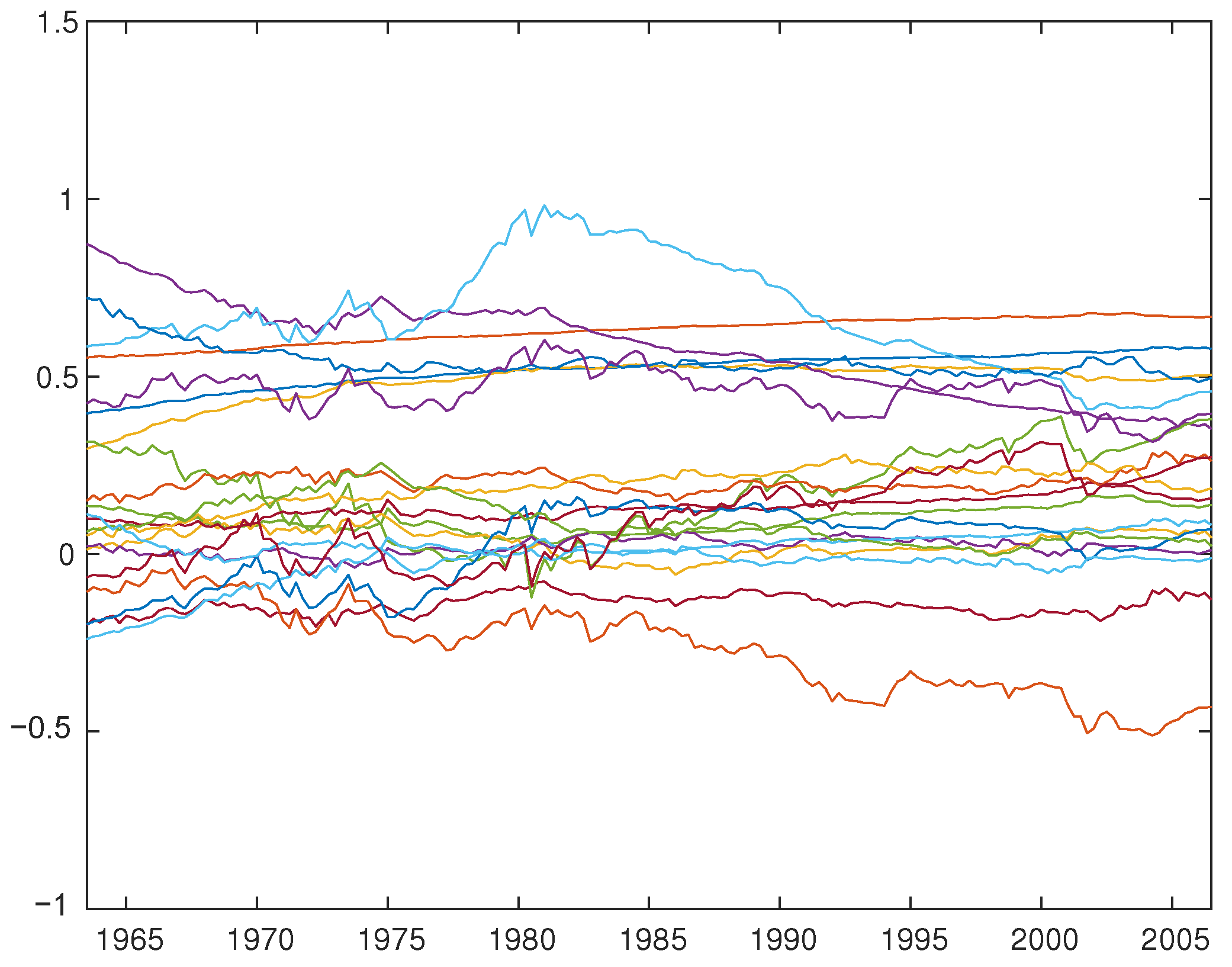
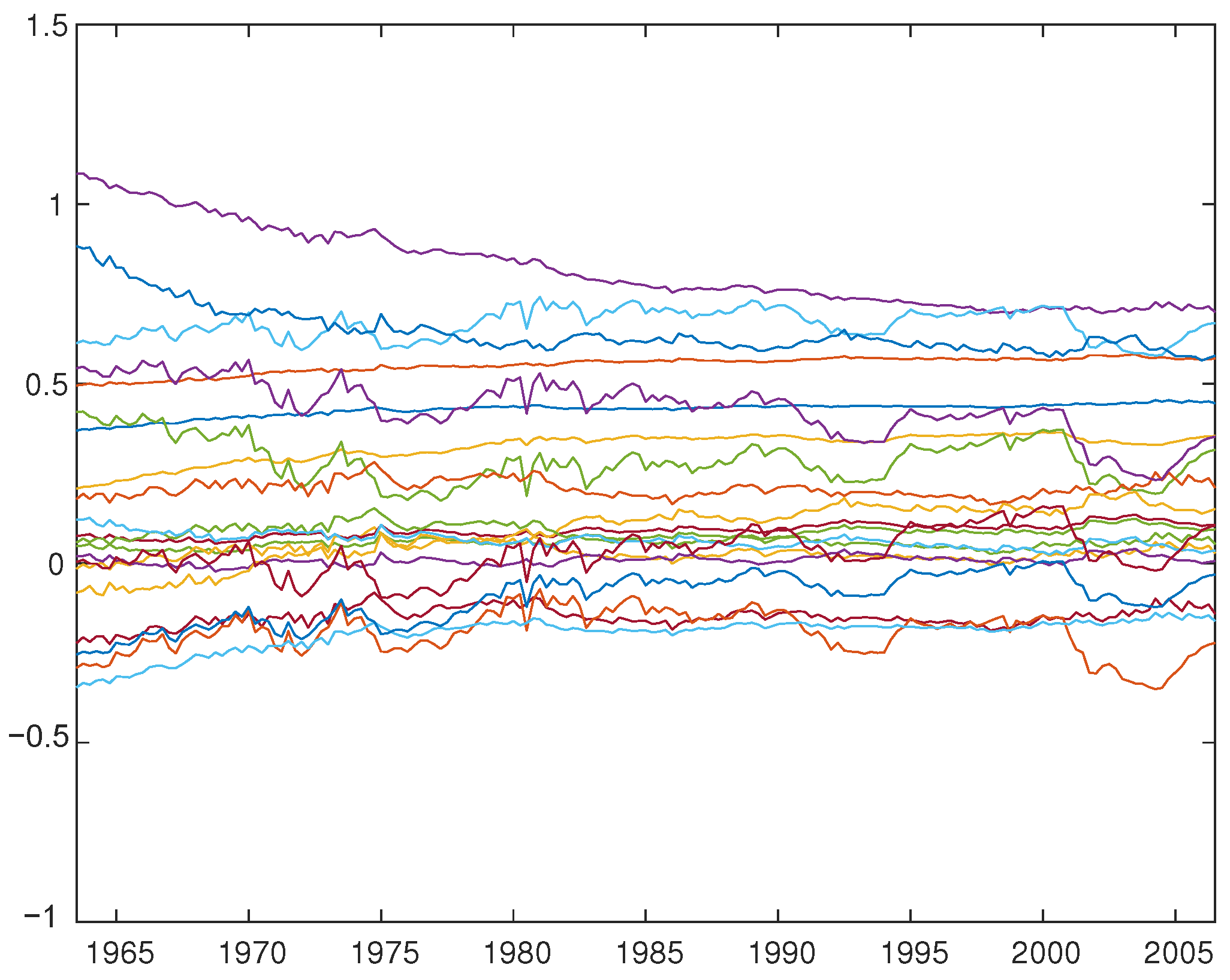
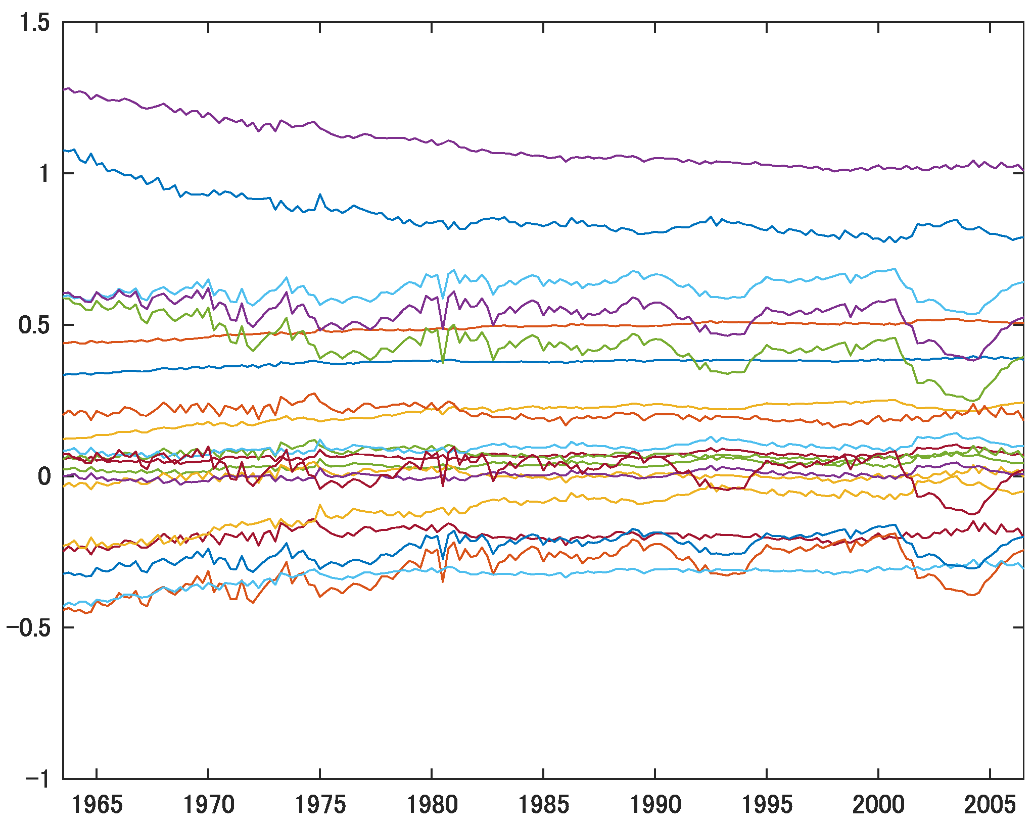
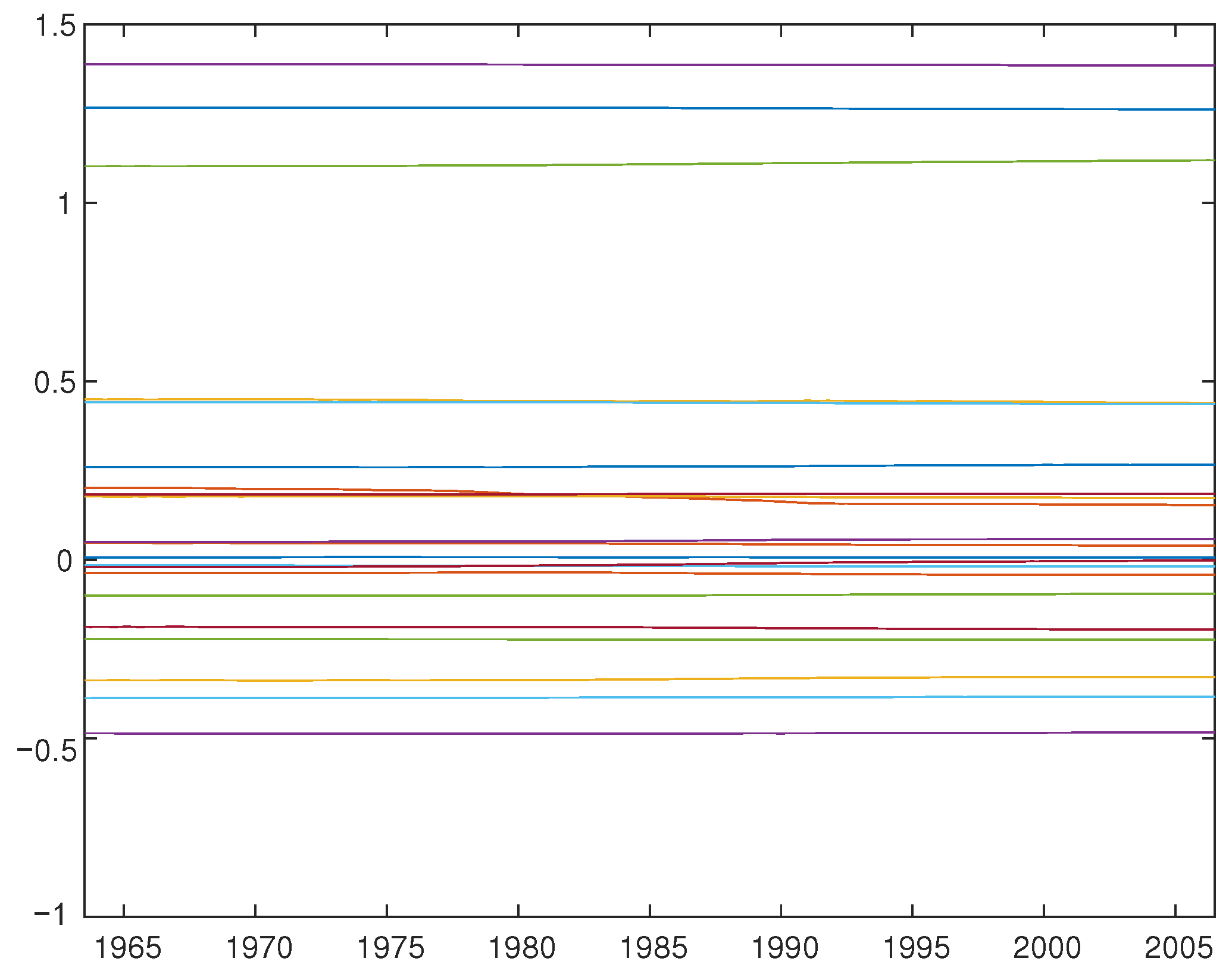
A number of studies that employ TV-VAR models, including Cogley and Sargent (2005) and Primiceri (2005), focus on recovering the structural parameters from the estimated reduced form. Although we do not aim to identify fundamental shocks or compute impulse responses, we present the estimated TV-VAR(2) parameter using OLS (Figure 1), FGLS (Figure 2 for 1FGLS, Figure 3 for 2FGLS’, and Figure 4 for 2FGLS), and the posterior mean of the time-varying approach using Primiceri’s (2005) method (Figure 5).12

While Primiceri’s (2005) Bayesian MCMC posterior means are virtually time-invariant and the estimates by 2FGLS’ are slightly more volatile, the estimates provided by OLS, 1FGLS and 2FGLS have much larger volatility.

Interestingly, as detailed in the supplementary appendix (available upon request), the coefficients on the interest rate vary noticeably over time, exhibiting distinct patterns in the early 1980s (dip), late 1990s (up) and early 2000s (down). Similar to Primiceri’s (2005) Bayesian posterior means, the intercepts (three time-varying coefficients) are largely stable over time. This finding is consistent with our simulation results. Overall, Primiceri’s (2005) Bayesian estimator for the time-varying parameter (${\beta }_t$) tends to have very small variation over time, resulting in virtually time-invariant parameters.13

6. Conclusions

The multivariate non-Bayesian regression-based or GLS-based approach for the time-varying parameter model is presented and assessed from a simulation aspect. Although this approach has already been theoretically justified and (at least partly) used by Ito et al. (2014 2016, 2021), it is shown that using the GLS-based approach has at least four advantages. First, this approach can produce equivalent estimates without needing Kalman filtering or smoothing; it is also applicable to a wide range of time-varying parameter models (e.g., TV-AR, TV-VAR, and TV-VEC models) by adjusting the regression matrix accordingly. Second, the GLS-based approach works reasonably well in practice in that it can estimate the time-varying parameters even when non-i.i.d. errors or non-Gaussian errors exist in the model. In particular, we find that GLS outperforms Primiceri’s (2005) Bayesian approach in recovering the true parameter values because it can take into account generally heteroskedastic error terms. The ability to deal with non-Gaussian errors is particularly important in empirical studies because it allows us to consider possible abrupt changes in time-varying parameters instead of gradual changes due to Gaussian errors. Remarkably, GLS can even outperform Primiceri’s (2005) Bayesian approach that is often employed to estimate the TV-VAR models. However, in practice, the most appropriate method (OLS, 1FGLS, 2FGLS or 2FGLS’) should be chosen depending on the sample size and SNR. More precisely, OLS is acceptable when the SNR is not far from one or the sample size is not small; otherwise, 2FGLS’ is recommended. The reason why the sample size and SNR are important for choosing the preferred of the three methods is that 1FGLS, 2FGLS and 2FGLS’ are not ideal GLS; hence, they cannot fully deal with the heterogeneity arising from our regression equation that includes both observation equation errors and state equation errors. However, because we do not maximize the unconditional likelihood function with respect to the variances of the errors and because 1FGLS, 2FGLS and 2FGLS’ are not ideal GLS, the true variances are imprecisely estimated, and our GLS-based approach does not suffer from the pile-up problem that often occurs with ML.

While our focus in this paper is the estimation method of relatively simple TV models, more flexible models, such as a TV-VAR with time-varying variances of the structural shocks, have a higher necessity for macroeconomic analysis. Extending our approach to such complex models is of great importance to both econometricians and macroeconomists.

References

- Bernanke, Ben S., and Ilian Mihov. 1998. Measuring monetary policy. Quarterly Journal of Economics 113: 869–902. [Google Scholar] [CrossRef] [Green Version]
- Chan, Joshua C. C., and Ivan Jeliazkov. 2009. Efficient simulation and integrated likelihood estimationin state space models. International Journal of Mathematical Modelling and Numerical Optimisation 1: 101–20. [Google Scholar] [CrossRef]
- Cogley, Timothy F., and Thomas J. Sargent. 2001. Evolving post-world war II u.s. inflation dynamics. NBER Macroeconomics Annual 16: 331–73. [Google Scholar] [CrossRef]
- Cogley, Timothy F., and Thomas J. Sargent. 2005. Drifts and volatilities: Monetary policies and outcomes in the post WWII US. Review of Economic Dynamics 8: 262–302. [Google Scholar] [CrossRef] [Green Version]
- Cogley, Timothy F., and Edward C. Prescott. 1976. Estimation in the presence of stochastic parameter variation. Econometrica 44: 167–84. [Google Scholar]
- Duncan, David B., and Susan D. Horn. 1972. Linear dynamic recursive estimation from the viewpoint of regression analysis. Journal of the American Statistical Association 67: 815–21. [Google Scholar] [CrossRef]
- Durbin, James, and Siem J. Koopman. 2012. Time Series Analysis by State Space Methods, 2nd ed. Oxford: Oxford University Press. [Google Scholar]
- Hamilton, James D. 1989. A new approach to the economic analysis of nonstationary time series and the business cycle. Econometrica 57: 357–84. [Google Scholar] [CrossRef]
- Hansen, Bruce E. 1992. Testing for parameter instability in linear models. Journal of Policy Modeling 14: 517–33. [Google Scholar] [CrossRef]
- Harvey, Andrew C. 1989. Forecasting, Structural Time Series Models and the Kalman Filter. Cambridge and New York: Cambridge University Press. [Google Scholar]
- Ito, Mikio, Akihiko Noda, and Tatsuma Wada. 2014. International stock market efficiency: A non-bayesian time-varying model approach. Applied Economics 46: 2744–754. [Google Scholar] [CrossRef] [Green Version]
- Ito, Mikio, Akihiko Noda, and Tatsuma Wada. 2016. The evolution of stock market efficiency in the us: A non-bayesian time-varying model approach. Applied Economics 48: 621–35. [Google Scholar] [CrossRef] [Green Version]
- Ito, Mikio, Akihiko Noda, and Tatsuma Wada. 2021. Time-varying comovement of foreign exchange markets: A GLS-based time-varying model approach. Mathematics 9: 849. [Google Scholar] [CrossRef]
- Koop, Gary, and Dimitris Korobilis. 2010. Bayesian multivariate time series methods for empirical macroeconomics. Foundations and Trends in Econometrics 3: 267–358. [Google Scholar] [CrossRef]
- Koopman, Siem J. 1997. Exact initial kalman filtering and smoothing for nonstationary time series models. Journal of the American Statistical Association 92: 1630–638. [Google Scholar] [CrossRef]
- Maddala, Gangadharrao S., and In-Moo Kim. 1998. Unit Roots, Cointegration, and Structural Change. Cambridge, New York: Cambridge University Press. [Google Scholar]
- McCausland, William J., Shirley Miller, and Denis Pelletier. 2011. Simulation smoothing for state-space models: A computational efficiency analysis. Computational Statistics & Data Analysis 55: 199–212. [Google Scholar]
- Perron, Pierre. 1989. The great crash, the oil price shock, and the unit root hypothesis. Econometrica 57: 1361–401. [Google Scholar] [CrossRef]
- Perron, Pierre, and Tatsuma Wada. 2009. Let’s take a break: Trends and cycles in us real gdp. Journal of Monetary Economics 56: 749–65. [Google Scholar] [CrossRef]
- Primiceri, Giorgio E. 2005. Time varying structural vector autoregressions and monetary policy. Review of Economic Studies 72: 821–52. [Google Scholar] [CrossRef]
- Sant, Donald T. 1977. Generalized least squares applied to time varying parameter models. Annals of Economic and Social Measurement 6: 301–14. [Google Scholar]
- Sargan, Dennis J., and Alok Bhargava. 1983. Maximum likelihood estimation of regression models with first order moving average errors when the root lies on the unit circle. Econometrica 51: 799–820. [Google Scholar] [CrossRef]
- Shephard, Neil G., and Andrew C. Harvey. 1990. On the probability of estimating a deterministic component in the local level model. Journal of Time Series Analysis 11: 339–347. [Google Scholar] [CrossRef]
- Tanaka, Katsuto. 2017. Time Series Analysis: Nonstationary and Noninvertible Distribution Theory, 2nd ed. Hoboken: John Wiley & Suns, Inc. [Google Scholar]
- Taylor, Stephen J. 2007. Modelling Financial Time Series, 2nd ed. Hackensack: World Scientific. [Google Scholar]
Figure 1.
The Estimated Time-Varying Parameters: OLS.
Figure 2.
The Estimated Time-Varying Parameters: 1FGLS.
Figure 3.
The Estimated Time-Varying Parameters: 2GLS’.
Figure 4.
The Estimated Time-Varying Parameters: 2GLS.