
A Joint Chow Test for Structural Instability

1
Department of Economics, University of Oxford & Institute of Economic Modelling & Nuffield College, Oxford OX1 1NF, UK
2
The World Bank, 1818 H Street NW, Washington DC 20433, USA
*
Author to whom correspondence should be addressed.
Econometrics 2015, 3(1), 156-186; https://0-doi-org.brum.beds.ac.uk/10.3390/econometrics3010156
Submission received: 19 December 2014
/
Revised: 6 February 2015
/
Accepted: 26 February 2015
/
Published: 12 March 2015
Abstract
:The classical Chow test for structural instability requires strictly exogenous regressors and a break-point specified in advance. In this paper, we consider two generalisations, the one-step recursive Chow test (based on the sequence of studentised recursive residuals) and its supremum counterpart, which relaxes these requirements. We use results on the strong consistency of regression estimators to show that the one-step test is appropriate for stationary, unit root or explosive processes modelled in the autoregressive distributed lags (ADL) framework. We then use the results in extreme value theory to develop a new supremum version of the test, suitable for formal testing of structural instability with an unknown break-point. The test assumes the normality of errors and is intended to be used in situations where this can be either assumed nor established empirically. Simulations show that the supremum test has desirable power properties, in particular against level shifts late in the sample and against outliers. An application to U.K. GDP data is given.
JEL classifications:
C221. Introduction
Identifying structural instability in models is of major concern to econometric practitioners. The Chow [1] tests are perhaps the most widely used for this purpose, but require strictly exogenous regressors and a break-point specified in advance. As such, a plethora of variants have been developed to meet different requirements. In this paper, we consider two generalisations: the one-step recursive Chow test, based on the sequence of studentised recursive forecast residuals; and its supremum counterpart. The pointwise test is frequently used and reported in the applied work, while the supremum test is new. Whereas Chow assumes a classical regression framework, practitioners typically use the one-step test to evaluate dynamic models, e.g., [2]. Further, since a series of such tests is usually presented graphically to the modeller, multiple testing issues arise, making it difficult to determine how many point failures may be tolerated. These two issues motivate the analysis that follows. First, in Theorem 6, we show that the pointwise statistic has the correct asymptotic distribution under fairly general assumptions about the generating process, including lagged dependent variables and deterministic terms. Second, we take advantage of the almost sure convergence proven earlier to construct a supremum version of the one-step test, applicable to detecting parameter change or the outlier at an unknown point in the sample. The supremum test offers several advantages useful to modellers: it is simple to compute and has a standard distribution under the null, which does not depend on the autoregressive parameter (even in the unit-root or explosive cases); it focuses attention on end-sample instability; and it is agnostic about the number of breaks, giving power against more complex forms of misspecification. These advantages incur certain costs: the test is not invariant to the distribution of errors (even asymptotically); and other tests are more powerful against particular alternatives.
The pointwise one-step Chow test is essentially the “prediction interval” test described by Chow, but computed recursively and over the sample (rather than at an a priori hypothesised change point). It first appears in PcGive Version 4.0 [3] as part of a suite of model misspecification diagnostics; a similar diagnostic graphic, the “one-step forecast test”, is provided in EViews ([4] p. 180). The idea of using residuals calculated recursively to test model misspecification dates to the landmark cumulated sum (CUSUM) and cumulated sum of squares (CUSUMSQ) tests [5,6], which are based on partial sums of (squared) recursive residuals and have since been generalised to models, including lagged dependent variables [7,8,9]. Unlike these tests, the one-step Chow test does not consider partial sums, but the sequence of recursive residuals itself; in effect, testing one-step-ahead forecast failure at each time step. As the following analysis shows, this approach leads to a different type of asymptotics, with a residual sequence behaving like i.i.d. random variables, rather than a partial sum of residuals behaving like a Brownian motion.
Examining the residual sequence to check the model specification is, of course, well established. The residuals can be either OLS residuals or recursive residuals, see [6,10]. The recursive residuals have two advantages over the OLS residuals: first, under the normal linear model with fixed regressors, they are identically and independently normal; second, they have a natural interpretation (in a time series setting) as forecast errors. Ironically, in typical time series settings, where the forecast error interpretation is most useful, the independence of the residuals does not hold due to the presence of lagged dependent variables, see [11]. This may lead to difficulties drawing firm conclusions from plotted pointwise test sequences and, thus, motivates the second part of this paper, which considers a supremum test.
The supremum test considers the maximum of the pointwise one-step tests, appropriately normalised. It is intended to reflect structural instability anywhere in the sample (with the early part excluded to allow consistent estimation). It relates to work on tests for either structural breaks or outliers, both at a possibly unknown time.
Perron [12] divides structural breaks tests into those that do not explicitly model a break, those that model one break and those that model multiple breaks. Our test joins the first category, which includes the already mentioned CUSUM and CUSUMSQ tests. (As an aside, Perron notes that these tests can suffer from the non-monotonicity of power against some alternatives. The risk of this is much reduced by using the one-step Chow statistics, since all parameters are estimated on a growing sub-sample.) The modelled break category includes, most prominently, the Quandt-Andrews (respectively, [13,14] supremum tests. These tests are complicated by a non-standard distribution (tabulated in [15]), but are nevertheless popular in practice, being implemented in several software packages. Our test is distinguished from these by not imposing any restrictions on the end-of-sample, so that end-of-sample instability may be detected. This feature is similar to [15], but a key distinction is that our test is agnostic about the number of breaks in the sample, a useful property in practice. It is also substantially simpler in implementation. Additionally, because the one-step tests behave like an i.i.d. process, the asymptotics differ from full-sample tests, like Quandt-Andrews, requiring the application of the extreme value theory of independent and weakly dependent sequences, rather than the suprema of random-walks.
Seen specifically as an outlier test, the supremum Chow test falls squarely within the tradition of [16], which, however, considers an unknown outlier in a classical setting. Outliers in the Box-Jenkins paradigm have attracted substantial interest, see [17,18,19]. These authors take a full-sample approach with stepwise elimination of outliers. Although effective in many cases, there is a risk of smearing/masking effects when multiple outliers are present, which is reduced with the recursive the test we present.
Surprisingly, the use of recursive residuals to detect outliers in time series data is relatively unexplored, although there is little doubt that they are used for this purpose in practice. Barnett and Lewis ([20] p. 330) comment that “[recursive residuals] would seem to have the potential for the study of outliers, although no major progress on this front is evident. There is a major difficulty in that the labelling of the observations is usually done at random, or in relation to some concomitant variable…”. This difficulty does not exist with time series, where there is a natural chronological labelling of observations. The section in the same book (at p. 396) on detecting outliers in time series is, nevertheless, notably brief, and recursive methods are not considered.
2. The Test Statistics
The one-step test applies to a linear regression:
with scalar, a k-dimensional vector of regressors and the errors independently and identically distributed. For such a regression, we can define the sequence of least squares estimators calculated over progressively larger subsamples,
along with the corresponding residual sums of squares
and recursive residual (or standardised one-step forecast error)
The one-step Chow test statistic, , is then defined as:
and can be expressed as:
Chow showed that in a classical Gaussian regression model, this statistic would have an exact distribution. We first extend this result to show that, for a general class of Gaussian autoregressive distributed lag (ADL) processes, converges in distribution to a random variable, so that, asymptotically, the additional dependence does not matter. This result means that comparing the pointwise statistic against an or distribution (as is typically done) is appropriate in large samples. However, it still leaves unresolved the difficulty that this test is generally reported graphically to detect parameter change with an unknown change point. To formally treat the problem of multiple testing that occurs in evaluating many pointwise statistics over the entire sample, we introduce a new supremum test based on the test statistic:
where g is an arbitrary function of T, such that .
To put the test statistics and the asymptotic analysis into perspective, it is useful to review some related, but also somewhat different statistics. The literature on adaptive control, also called tracking, comes to mind, although it does not appear to be applied much in econometrics. It is concerned with tracking the sum of squares innovations. The aim is then to show that:
vanishes. A discussion for a non-explosive autoregressive setup without deterministic terms is given in [21,22]. Asymptotic distribution theory does not seem to be discussed. The reason that the tracking result does not extend to the explosive case is that the residuals are not normalised by the “hat” matrix, in contrast to the residuals in Equation (4). Normalisation by the “hat” matrix also gives excellent finite-sample properties; see Section 5.
The Chow statistic in Equation (5) also involves scaling by a residual variance estimator, so that the asymptotic distribution is free of nuisance parameter; see Theorem 6 below. More fundamentally, the present analysis is concerned with the Chow statistic for individual observations rather than sums, and it will therefore involve extreme value theory.
Another related test that is used in econometrics is the CUSUMSQ test based on the statistic:
or a similar statistic based on least squares residual variance estimates instead of sums of squared recursive residuals. This test statistic is aimed at detecting non-constancy in the innovation variance rather than detecting individual outliers. Again, it includes normalisation by the “hat” matrix. Distribution theory is discussed in [7,8] for the stationary case and in [9] for general autoregressions, which are possibly explosive and with deterministic terms.
3. Model and Assumptions
We consider the behaviour of the test statistic for ADL models with arbitrary deterministic terms, a class that includes by restriction many commonly-posited economic relationships, see ([23] Chapter 7). For the purpose of analysis, we assume that the true data generating model can be represented as a vector autoregression (VAR).
We observe a p-dimensional time series . We model the series by partitioning as , where is univariate and is of dimension , and then consider the regression of on the contemporaneous , lags of both and and a deterministic term . That is,
In order to specify the joint distribution of , we assume that follows the vector autoregression:
with the deterministic term given by:
The deterministic term follows the approach of [24,25] and may include, for example, a constant, a linear trend or periodic functions, such as seasonal dummies. The matrix has characteristic roots on the unit circle. For example,
will generate a constant and a biannually dummy. The term is assumed to have linearly-independent coordinates, formalised as follows.
Assumption 1. and
We assume the VAR innovations form a martingale difference sequence satisfying the assumption below. The requirement that the innovations have finite moments just beyond 16 stems from a problem with controlling unit root processes, see ([25] Remark 9.3). In the present analysis, this constraint emerges in Lemma 12 (i) and is transmitted via Lemma 13 (iv) to Lemma 16. If and the geometric multiplicity of roots in unity equals their algebraic multiplicity (including , but excluding processes), this could be improved to finite moments greater than four using the result of [26].
Assumption 2. is a martingale difference sequence with respect to the natural filtration , so . The initial values are -measurable and:
This assumption also excludes the possibility that the innovations could be heteroscedastic, a common assumption in financial modelling (e.g., autoregressive conditional heteroscedastic, ARCH), but also an increasingly relevant property in macroeconomic work, particularly in light of the “Great Moderation” period [27] and subsequent period of the “Global Financial Crisis”. The assumption indicates that such heteroscedasticity should be modelled.
We permit nearly all possible values of the autoregressive parameters in Equation (11), excluding only the case of singular explosive roots, which can only arise for a VAR with and multiple explosive roots, see [28] for a discussion. We can express the restriction in terms of the companion matrix:
Assumption 3. The explosive roots of have geometric multiplicity of unity. That is, for all complex λ with , .
Additionally, we require that the innovations in the ADL regression are martingale differences.
Assumption 4. Let be the sigma field over and . Then, is a martingale difference sequence, i.e., .
Finally, the one-step statistic is such that a distributional assumption must be made in order to derive the limiting distribution of the statistic (since the statistic is an estimate of a single error term, we cannot take advantage of a central limit theorem). Similarly, since the analysis of the supremum statistic will rely on extreme value theory, we must impose distributional and independence assumptions on the ADL innovations , in order to uniquely determine the norming sequences applied in Lemma 9. We assume normality, which may result from joint normality in the underlying VAR process and is tested, in practice, under the above assumptions, see [29].
Assumption 5. .
4. Main Results
We must briefly examine the decomposition of the process used in the proofs in order to elucidate the first main result in the explosive case (in the non-explosive case, this decomposition becomes trivial). A two-way decomposition allows us to express separately certain terms that arise in connection with the explosive component of the process. Group the regressors by defining:
and then write Equation (11) in companion form, so that:
Then, there exists a regular real matrix to block diagonalize (see the elaboration in Section 3 of [25]), so that the process can be decomposed into non-explosive and explosive components, and , respectively. We have:
with and having eigenvalues inside or on, and outside, the unit circle, respectively.
The first theorem states that the test statistic is almost surely close to a related process in the innovations, , under multiple assumptions. This result does not require the normality of Assumption 5.
Theorem 6. Under Assumptions 1, 2, 3 and 4,
where:
and is as in Equation (16), and as in [25] (Corollaries 5.3 and 7.2), and , with almost surely positive definite.
Having established pointwise convergence almost surely, we use an argument based on Egorov’s theorem to establish the convergence of the supremum of a subsequence. Both the subsequence itself and the lead-in period must grow without bound, to allow the regression estimates to converge.
Lemma 7. Suppose . Then:
where is an arbitrary function of T, such that .
Now, if an appropriately normalised expression in the maximum over can be shown to converge in distribution, then so will the supremum statistic, with the same normalisation, by asymptotic equivalence. We show that, under the assumption of independent and identical Gaussian innovations, , appropriately normalised, does indeed converge to the Gumbel extremal distribution (as ), which has distribution function:
A useful property of the Gumbel distribution is the following simple monotonically decreasing transformation to a variable, allowing standard distributions to be used:
In showing the above convergence, we rely on Theorem 1 of Deo [30], and its corollary, showing that the extremal distribution of the absolute values of a Gaussian sequence is the same in the stationary dependent and independent cases. However, Deo’s Lemma 1 gives an incorrect statement of the norming sequences. Here, we state the correct sequences, adopting the notation of Deo (proof in Section A.6).
Lemma 8. Let be independent Gaussian random variables with mean zero and variance one. Let . Then, converges in distribution to Λ, where and .
The original gives .
Deo’s result can then be applied to defined in Equation (18).
Lemma 9. Under Assumption 5,
where:
and Λ is a random variable distributed according to the Gumbel (Type 1) law.
Combining these lemmas gives our main result, that with independent and identically Gaussian innovations, an appropriate normalisation of the supremum one-step Chow test converges in distribution to the Gumbel extremal distribution.
Theorem 10. Under Assumptions 1, 2, 3, 4 and 5, with some ,
where is the one-step Chow statistic defined in Equation (5) and:
and Λ is a random variable distributed according to the Gumbel distribution Equation (20).
As a simple corollary, we can transform the test using Equation (21), so that it may be compared against a more readily-available distribution.
Corollary 11. Under the same assumptions, . A test based on this result should reject for small values of the statistic.
5. Finite-Sample Corrections
In practice, we find by simulation that the test as specified above is over-sized in small samples. To minimise this, we suggest two corrections. For the first correction, we observe that the one-step statistics appear to be distributed close to (as indeed, they are exactly in the classical case) and so use the following transformation to bring the statistics closer to the asymptotic chi-squared distribution:
where and are the and distribution functions, respectively. This first correction results in a test that tends to under-correct, largely a result of relatively slow convergence to the limiting Gumbel distribution. We find that the test performs better if simply compared with the finite maximal distribution, assuming the independence and identical distribution of the test statistics (the first assumption holding only in the limit and in the absence of an explosive component and the second holding only in the limit). That is, we approximate the distribution of the maximum, , by:
This forms the basis of the finite adjusted sup-Chow test (), with rejection in the right tail. Note that in this case, no centring or scaling is required, because the null distribution itself depends on T.
6. Simulation Study
We present the results of four simulation experiments done in Ox [31]: size; distributional sensitivity; power against mean shifts; and power against outliers. All of the simulations are done first for a first order autoregression and then for an autoregressive distributed lag model.
6.1. Autoregressive Data-Generating Process
Consider the following data-generating process:
Where not otherwise stated, we set and . The number of Monte Carlo repetitions and the implied Monte Carlo standard error, , are indicated in table captions.
The regression model is that of an first order autoregression. It includes an intercept unless otherwise stated. The five tests computed and presented in the tables are: the asymptotic sup-Chow test (); the corrected sup-Chow test (); the [13] sup-F test (); an outlier test based on the OLS residuals (); and the [32] test for normality (Φ). The nominal size is unless otherwise stated.
The two sup-Chow tests are described in Theorem 10 and Equation (28), respectively; for the function , we use . The sup-F test is a linear regression form of Andrews’ sup-W (Wald) test with 15% trimming, as used for the simulations in [33] and implemented in EViews 7 by the command ubreak. It is the maximum of the Chow F-tests calculated over break points , such that for each break point λ, under the alternative, the model is estimated separately for each subsample ( and …T), whereas under the hypothesis, the model is estimated for the full sample. The null distribution is given by asymptotic approximation to a non-standard distribution with simulated critical values given in [15]. The sup- test examines the maximum of the squared full-sample OLS residuals, externally studentised as in ([34] s. 2.2.9); that is, residual t is normalised using an estimate of the error variance that excludes residual t itself. These squared statistics are distributed under normality of the errors, but not independent; hence, the use of the Bonferroni inequality to find significance levels is recommended by [34]. We find in simulation that, despite dependence, the exact maximal distribution of T independent random variables is a reasonable choice for the sample sizes and processes we consider, except those that are near-unit-root. Finally, in experiments where we wish to evaluate the performance of the sup-Chow test conditional on residuals having satisfied a normality test, we use the [32] test of the OLS residuals.
In the first experiment (Table 1), we vary the autoregressive parameter through the stationary, unit-root and explosive regions and consider the effect of either including or excluding an intercept from the model. As noted above, the test is uniformly oversized. The test is correctly sized and approximately similar, with simulated size varying very little across the parameter space. There is some tendency towards inflated sizes under near-unit-root processes when an intercept is included in the model, but the extent of this is quite limited (7% simulated size). The key consequence of this result is that it is not necessary to know a priori where the autoregressive parameter lies to effectively apply the test, avoiding a potential circularity in model construction.
In simulations that are not reported here, we also investigated the test. This test is not valid in the non-stationary case. Thus, the same patterns were seen, albeit with a larger effect. The simulated size is as high as 44% in the unit root case.

Table 1.
Simulated rejection frequency for and under the Gaussian autoregression in Equation (29). 200,000 repetitions, .
| T | Autoregressive Coefficient (α) | ||||||||
|---|---|---|---|---|---|---|---|---|---|
| −1.03 | −1.00 | −0.50 | 0.00 | 0.50 | 0.90 | 1.00 | 1.03 | ||
| 5% Nominal Size | |||||||||
| Intercept included in model (M1) | |||||||||
| 25 | 14.52 | 14.44 | 13.92 | 14.40 | 15.82 | 19.28 | 19.86 | 20.21 | |
| 5.30 | 5.26 | 5.01 | 5.24 | 5.78 | 7.28 | 7.59 | 7.75 | ||
| 50 | 12.80 | 12.72 | 12.32 | 12.60 | 13.50 | 16.13 | 16.97 | 17.43 | |
| 5.17 | 5.15 | 4.92 | 5.05 | 5.38 | 6.52 | 7.00 | 7.27 | ||
| 100 | 10.43 | 10.41 | 10.15 | 10.36 | 10.73 | 12.34 | 13.27 | 13.85 | |
| 5.09 | 5.05 | 4.95 | 5.00 | 5.08 | 5.82 | 6.38 | 6.74 | ||
| No intercept included in model (M2) | |||||||||
| 25 | 15.28 | 15.23 | 14.51 | 14.49 | 14.62 | 15.11 | 15.33 | 15.39 | |
| 5.49 | 5.46 | 5.20 | 5.19 | 5.23 | 5.44 | 5.49 | 5.53 | ||
| 50 | 13.17 | 13.12 | 12.72 | 12.72 | 12.71 | 13.01 | 13.20 | 13.21 | |
| 5.33 | 5.29 | 5.06 | 5.03 | 5.09 | 5.20 | 5.26 | 5.27 | ||
| 100 | 10.64 | 10.60 | 10.27 | 10.31 | 10.34 | 10.42 | 10.62 | 10.63 | |
| 5.17 | 5.12 | 5.02 | 4.99 | 5.01 | 5.03 | 5.13 | 5.16 | ||
| 1% Nominal Size | |||||||||
| No intercept included in model (M1) | |||||||||
| 25 | 6.30 | 6.29 | 5.98 | 6.24 | 7.06 | 8.87 | 9.16 | 9.33 | |
| 1.09 | 1.10 | 1.04 | 1.07 | 1.24 | 1.64 | 1.75 | 1.79 | ||
| 50 | 4.77 | 4.77 | 4.56 | 4.70 | 5.16 | 6.44 | 6.83 | 7.04 | |
| 1.08 | 1.08 | 1.02 | 1.06 | 1.15 | 1.45 | 1.57 | 1.60 | ||
| 100 | 3.36 | 3.36 | 3.24 | 3.31 | 3.47 | 4.22 | 4.59 | 4.74 | |
| 1.05 | 1.05 | 1.02 | 1.02 | 1.04 | 1.21 | 1.36 | 1.43 | ||
| No intercept included in model (M2) | |||||||||
| 25 | 6.71 | 6.69 | 6.25 | 6.22 | 6.34 | 6.59 | 6.71 | 6.73 | |
| 1.16 | 1.15 | 1.06 | 1.04 | 1.06 | 1.12 | 1.18 | 1.19 | ||
| 50 | 4.98 | 4.97 | 4.70 | 4.69 | 4.78 | 4.90 | 4.95 | 4.95 | |
| 1.12 | 1.11 | 1.04 | 1.05 | 1.05 | 1.07 | 1.10 | 1.09 | ||
| 100 | 3.41 | 3.37 | 3.24 | 3.24 | 3.25 | 3.33 | 3.39 | 3.40 | |
| 1.06 | 1.05 | 1.02 | 1.01 | 1.00 | 1.00 | 1.03 | 1.04 | ||
The second experiment evaluates the sensitivity of the test to failures of Assumption 5, in particular the non-normality of the errors. Table 2 presents simulated sizes for both the and tests under a range of error distributions. The former is very sensitive to departures from normality, while the latter is not. In the second part of the table we consider a further scenario, in which a model builder runs the structural instability tests only if a test for normal residuals is not rejected. This yields three additional tests, the normality test Φ and the and tests, each conditional on the normality hypothesis having not been rejected. We also consider joint tests and that first tests normality and then tests for break if normality cannot be rejected. As the table illustrates, some size distortion remains, but the inflation of the unconditional test is largely controlled in the conditional case. As noted in Section 8 below, we recommend using the test in this way if the normality of the errors cannot be safely assumed.
Table 2.
Simulated rejection frequency for and , possibly combined with normality test Φ, under autoregression in Equation (29) with various error distributions. 50,000 repetitions, .
| T | Error Distribution | |||||
|---|---|---|---|---|---|---|
| Φ | ||||||
| Unconditional tests | ||||||
| 50 | 5.0 | 6.6 | 15.0 | 28.8 | 40.9 | |
| 6.0 | 6.0 | 6.0 | 5.9 | 6.3 | ||
| 100 | 5.0 | 7.4 | 22.2 | 45.0 | 59.9 | |
| 4.9 | 5.0 | 4.9 | 4.7 | 4.9 | ||
| Joint tests | ||||||
| 50 | Φ | 4.9 | 6.7 | 19.0 | 41.0 | 95.1 |
| 3.4 | 3.9 | 6.2 | 8.0 | * 7.4 | ||
| 6.0 | 6.0 | 6.1 | 6.0 | * 6.7 | ||
| 8.1 | 10.4 | 24.0 | 45.8 | * 95.5 | ||
| 10.6 | 12.3 | 23.9 | 44.6 | * 95.4 | ||
| 100 | Φ | 4.8 | 7.6 | 28.7 | 63.0 | 100.0 |
| 3.3 | 4.2 | 7.2 | 8.6 | |||
| 5.0 | 5.0 | 5.0 | 4.9 | |||
| 8.0 | 11.5 | 33.9 | 66.2 | * 100.0 | ||
| 9.5 | 12.2 | 32.3 | 64.8 | * 100.0 | ||
The third experiment considers the power of the tests against a single shift in the mean level of the process. The data generating process is:
and we allow γ and τ to vary as presented. The regression model remains a first order autoregression with an intercept. The level shift is therefore not modelled. Table 3 shows simulated sizes for the unconditional tests as in the previous experiment. We note that the test performs well for a break at mid-sample, but is outperformed by the test for breaks occurring near the end of the sample. We also consider conditional tests as in the previous experiment. There are two main observations: firstly, the normality test is increasingly likely to reject as the break magnitude becomes large; but secondly, the test still has power (attenuated by around one-half) to detect the break in this case.
Table 3.
Simulated rejection frequency for and , possibly combined with normality test Φ, under the process in Equation (30) with a break of magnitude γ at time τ. 50,000 repetitions, .
| T | Break Timing (τ) | |||||||
|---|---|---|---|---|---|---|---|---|
| 0.5T | T-2 | T-1 | ||||||
| Post-Break Constant (γ) | ||||||||
| 0.0 | 2.0 | 4.0 | 2.0 | 4.0 | 2.0 | 4.0 | ||
| Unconditional tests | ||||||||
| 25 | 5.5 | 13.7 | 51.2 | 21.0 | 78.7 | 16.0 | 70.3 | |
| 10.3 | 90.4 | 99.9 | 19.9 | 44.8 | 14.1 | 28.1 | ||
| 50 | 5.2 | 17.1 | 67.6 | 18.6 | 83.2 | 13.3 | 69.9 | |
| 6.0 | 99.8 | 100.0 | 10.2 | 34.5 | 7.1 | 11.5 | ||
| 100 | 5.1 | 20.0 | 77.9 | 16.1 | 84.2 | 11.5 | 67.6 | |
| 4.9 | 100.0 | 100.0 | 7.2 | 31.2 | 5.4 | 7.4 | ||
| Joint tests | ||||||||
| 25 | Φ | 5.1 | 4.3 | 15.6 | 9.6 | 37.9 | 9.9 | 53.9 |
| 3.8 | 12.5 | 45.3 | 14.8 | 66.7 | 9.4 | 38.3 | ||
| 10.2 | 90.4 | 99.9 | 19.6 | 52.1 | 13.1 | 22.6 | ||
| 8.7 | 16.2 | 53.8 | 22.9 | 79.4 | 18.4 | 71.5 | ||
| 14.8 | 90.8 | 99.9 | 27.3 | 70.3 | 21.7 | 64.3 | ||
| 50 | Φ | 4.8 | 4.4 | 17.0 | 11.1 | 61.9 | 9.5 | 58.6 |
| 3.5 | 15.7 | 62.6 | 11.3 | 58.6 | 7.2 | 31.1 | ||
| 6.0 | 99.8 | 100.0 | 9.8 | 33.9 | 6.9 | 9.0 | ||
| 8.2 | 19.4 | 69.0 | 21.1 | 84.2 | 16.1 | 71.5 | ||
| 10.6 | 99.9 | 100.0 | 19.8 | 74.8 | 15.8 | 62.3 | ||
| 100 | Φ | 4.7 | 4.2 | 15.6 | 11.2 | 74.7 | 8.5 | 57.4 |
| 3.4 | 18.7 | 74.7 | 8.9 | 43.5 | 6.4 | 28.4 | ||
| 4.9 | 100.0 | 100.0 | 6.8 | 19.3 | 5.4 | 6.3 | ||
| 8.0 | 22.1 | 78.7 | 19.1 | 85.7 | 14.4 | 69.5 | ||
| 9.4 | 100.0 | 100.0 | 17.2 | 79.6 | 13.5 | 60.0 | ||
The fourth experiment (Table 4) considers the power of the tests against a single innovation outlier at the process mid-point. The data generating process is:
and we allow α and δ to vary. Both tests presented have similar power in most circumstances, with an outlier larger than three-times the error standard deviation being detected with useful frequency. The OLS-based test has slightly better power than the Chow test. The conditional evaluations show that both tests retain power in situations where the normality test is not rejected.
Table 4.
Simulated rejection frequency for and , possibly combined with normality test Φ, under the process in Equation (31) with a break of magnitude δ. 50,000 repetitions, .
| α | T | Outlier Magnitude (δ) | ||||||
|---|---|---|---|---|---|---|---|---|
| 0.0 | 1.0 | 2.0 | 3.0 | 4.0 | 5.0 | |||
| Unconditional tests | ||||||||
| 0.5 | 50 | 5.5 | 5.8 | 10.6 | 28.7 | 58.7 | 84.9 | |
| 4.7 | 5.0 | 10.5 | 31.8 | 66.2 | 90.7 | |||
| 100 | 5.2 | 5.5 | 9.8 | 28.1 | 61.1 | 87.9 | ||
| 4.8 | 5.1 | 9.8 | 29.9 | 65.1 | 90.8 | |||
| 0.9 | 50 | 6.6 | 7.0 | 12.0 | 30.2 | 59.7 | 85.3 | |
| 4.7 | 4.9 | 10.3 | 31.3 | 65.5 | 90.3 | |||
| 100 | 5.9 | 6.3 | 10.8 | 28.9 | 61.4 | 87.9 | ||
| 4.9 | 5.1 | 9.8 | 29.7 | 64.9 | 90.6 | |||
| Joint tests | ||||||||
| 0.5 | 50 | Φ | 4.9 | 5.0 | 9.6 | 27.7 | 59.3 | 86.6 |
| 3.8 | 4.0 | 5.8 | 10.8 | 18.0 | 25.6 | |||
| 2.2 | 2.4 | 4.0 | 10.3 | 22.7 | 36.8 | |||
| 8.5 | 8.8 | 14.8 | 35.5 | 66.6 | 90.0 | |||
| 7.0 | 7.3 | 13.2 | 35.2 | 68.5 | 91.5 | |||
| 100 | Φ | 4.8 | 5.0 | 8.7 | 25.0 | 57.1 | 86.0 | |
| 3.5 | 3.7 | 5.2 | 11.0 | 20.9 | 32.0 | |||
| 2.7 | 2.8 | 4.4 | 10.9 | 24.3 | 40.0 | |||
| 8.1 | 8.5 | 13.4 | 33.2 | 66.1 | 90.5 | |||
| 7.3 | 7.7 | 12.7 | 33.2 | 67.5 | 91.6 | |||
| 0.9 | 50 | Φ | 4.9 | 5.1 | 9.4 | 27.1 | 58.6 | 85.9 |
| 4.9 | 5.2 | 7.3 | 13.1 | 21.6 | 30.6 | |||
| 2.2 | 2.3 | 4.0 | 10.3 | 22.6 | 37.5 | |||
| 9.5 | 10.0 | 16.0 | 36.6 | 67.5 | 90.2 | |||
| 6.9 | 7.2 | 13.0 | 34.6 | 68.0 | 91.2 | |||
| 100 | Φ | 4.7 | 5.0 | 8.6 | 24.7 | 56.8 | 85.8 | |
| 4.2 | 4.4 | 6.2 | 12.2 | 22.2 | 33.6 | |||
| 2.7 | 2.8 | 4.4 | 10.9 | 24.2 | 39.5 | |||
| 8.7 | 9.2 | 14.3 | 33.8 | 66.4 | 90.6 | |||
| 7.3 | 7.6 | 12.6 | 32.9 | 67.2 | 91.4 | |||
6.2. Autoregressive Distributed Lag Data-Generating Process
We consider a bivariate data-generating process, written in triangular equilibrium correction form as
where . The characteristic roots of the system are ψ and . When , the model is cointegrated. When , the model is stationary. In both cases, is stationary.
We then fit the univariate autoregressive distributed lag model
and investigate the residuals using the Chow statistics.
The first experiment (Table 5) evaluates the size of the Chow tests. Here, ψ varies, while in the data generating process. The results are in line with those seen for the autoregressive situation in Table 1. The second experiment is not done in this situation.
| T | Autoregressive Coefficient (ψ) | ||||
|---|---|---|---|---|---|
| 0.25 | 1.00 | ||||
| 50 | 15.0 | 16.3 | |||
| 6.1 | 6.7 | ||||
| 100 | 11.6 | 12.2 | |||
| 5.4 | 5.8 | ||||
The third experiment (Table 6) evaluates the power of the Chow tests against a single shift in the mean level. This is done by replacing ν by in the data generating process Equation (32). The results are in line with those seen for the autoregressive situation in Table 3: There is good size control. The power is nearly uniform in ψ and comparable to the power reported in Table 3.
The fourth experiment (Table 7) evaluates the power of the Chow tests against a single innovation outlier at the process mid-point. This is done by replacing ν by in the data generating process Equation (32). The results are in line with those seen for the autoregressive situation in Table 4.
| ψ | Break Timing(τ) | |||||||
|---|---|---|---|---|---|---|---|---|
| 0.5T | T-2 | T-1 | ||||||
| Post-Break Constant (ν) | ||||||||
| 0.0 | 2.0 | 4.0 | 2.0 | 4.0 | 2.0 | 4.0 | ||
| 0.25 | 6.1 | 16.3 | 64.6 | 19.7 | 83.2 | 13.8 | 68.2 | |
| Φ | 4.9 | 6.8 | 34.1 | 10.9 | 61.8 | 9.1 | 54.9 | |
| 4.5 | 13.4 | 51.2 | 12.7 | 58.8 | 8.4 | 33.1 | ||
| 9.2 | 19.3 | 67.8 | 22.2 | 84.3 | 16.7 | 69.8 | ||
| 1.00 | 6.7 | 16.0 | 62.0 | 19.4 | 81.2 | 14.2 | 67.2 | |
| Φ | 5.0 | 6.0 | 25.1 | 9.7 | 54.5 | 8.7 | 51.8 | |
| 5.3 | 13.7 | 52.6 | 13.5 | 60.8 | 9.1 | 35.2 | ||
| 10.0 | 18.9 | 64.5 | 21.9 | 82.2 | 17.0 | 68.8 | ||
| ψ | Outlier Magnitude (ν) | ||||||
|---|---|---|---|---|---|---|---|
| 0.0 | 1.0 | 2.0 | 3.0 | 4.0 | 5.0 | ||
| 0.25 | 6.1 | 6.3 | 10.4 | 25.5 | 53.0 | 79.1 | |
| Φ | 4.9 | 5.2 | 9.1 | 25.4 | 55.4 | 83.1 | |
| 4.5 | 4.6 | 6.3 | 10.8 | 17.5 | 24.8 | ||
| 9.2 | 9.6 | 14.8 | 33.5 | 63.2 | 87.3 | ||
| 1.00 | 6.7 | 7.1 | 11.0 | 25.4 | 51.5 | 77.4 | |
| Φ | 5.0 | 5.3 | 9.3 | 25.9 | 55.9 | 83.5 | |
| 5.3 | 5.5 | 7.1 | 11.7 | 18.5 | 26.0 | ||
| 10.0 | 10.5 | 15.7 | 34.6 | 64.1 | 87.8 | ||
7. Empirical Illustration
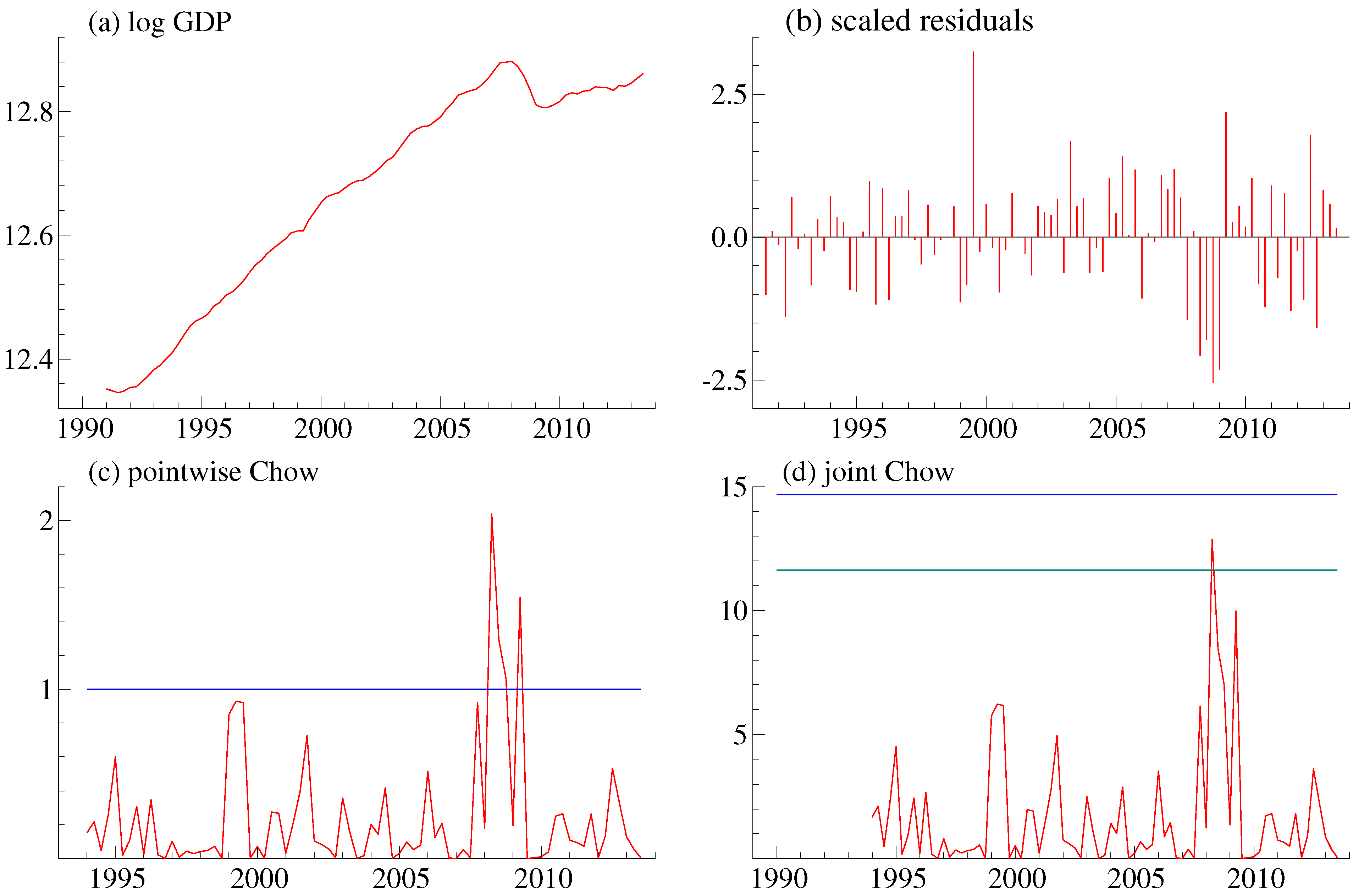
As an empirical illustration, consider log quarterly U.K. gross domestic product1, y, say, for the period 1991:1 to 2013:3. This gives a total sample length of 91, of which two observations are held back as initial values. The data is provided as supplementary material. Figure 1a shows the series.
An autoregression with two lags, an intercept and a linear trend is fitted to the data:
Figure 1.
U.K. GDP series. (a) Series in logs; (b) scaled residuals; (c) pointwise one-step Chow tests; the horizontal line is the 1% critical value; (d) simultaneous Chow test; the horizontal lines are the 1% (top) and 5% (bottom) critical values.
Figure 1.
U.K. GDP series. (a) Series in logs; (b) scaled residuals; (c) pointwise one-step Chow tests; the horizontal line is the 1% critical value; (d) simultaneous Chow test; the horizontal lines are the 1% (top) and 5% (bottom) critical values.

The specification tests in Equation (36) are a cumulant-based test for normality and a test for autocorrelated residuals. They are valid for non-stationary autoregressive distributed lag models; see [29,35,36]. These specification tests do not indicate particular problems with the model. The specification test in Equation (37) is the supremum Chow test from Equation (27) evaluated according to the finite sample approximation Equation (28). This indicates a specification problem that is worst for 2008:2. A graphical version of this test is discussed below.
Figure 1b shows the scaled residuals. There appears to be clustering of first positive and then negative residuals around the start of the financial crisis in 2006–2009. This tendency is, however, not sufficient to tricker the specification tests for autocorrelation and non-normality in Equation (36).
Figure 1c shows pointwise one-step Chow tests. This is the standard output from PcGive. The scale is a probability scale, where the horizontal line indicates the critical value for pointwise tests at a 1% level. The exact nature of the probability scale is not documented in [37]. This plot represents pointwise tests based on 79 statistics with an unclear correlation structure. Thus, researchers have traditionally interpreted this plot with a grain of salt; see ([38] p.197). In this plot, there is a cluster of pointwise rejections, so it would seem prudent to question the stability of the model.
Figure 1d shows the Chow statistics (see Equation (27)), along with horizontal lines indicating the critical values of simultaneous 5% and 1% tests. These are computed according to the finite sample approximation Equation (28). The maximum of the test statistics is 12.9; see Equation (37). This is between the 5% and the 1% critical levels of 11.6 and 14.7, respectively. Thus, with a 5% level, it would seem prudent to question the stability of the model.
What could be done to remedy the situation? The usual answer is to inspect the data, think about the economic context and the economic question of interest and update the empirical model accordingly. While the economic question is vague in this illustration, the context of the specification problem is the financial crisis. In 2008, there is downward shift both in productivity and in growth rates. How big these effects were remains unclear, and so, the Office of National Statistics keeps revising the data for this period; see [39,40]. Now, one way to capture the downward shift in productive and growth rates is to use an impulse indicator and a step indicator. This gives the model:
The formal asymptotic theory does not cover this situation with dummies. We proceed with these results nonetheless. The specification tests (39), (40) for the new model (38) are clearly better than the tests (37), (37) for the original model (35). An asymptotic theory for this type of iterative specification of a regression model is given in [41].
It is worth noting how the plot Figure 1d is computed. First, is computed using Equation (5) for , so that and . This can be done easily using standard regression techniques. For instance, to compute , run a regression including over the sample , including a dummy for Observation 11. Then, is the F-statistic for testing the absence of the dummy variable. Secondly, is computed from by first transforming using the distribution function, with and in this case, and then by the inverse of G, the distribution function. The critical values are computed according to the finite sample approximation (28). For instance, for , then , so that .
8. Conclusions
We advocate the sup-Chow test as a general misspecification test to be used as part of an iterative modelling strategy. It is a relatively simple transformation of the existing one-step Chow test (or, similarly, the EViews one-step forecast test), with a standard and easily calculated null distribution, which does not vary substantially in the AR(1) parameter space. We anticipate that it would be used as one of a battery of tests (including the normality of residuals); rejection would draw the modeller’s attention to the pointwise plot, which would help identify the cause and timing of the failure.
By construction, the test is sensitive to parameter changes and outliers and is somewhat agnostic about the timing and number of these breaks. This makes it useful against a variety of simple and complex misspecification types. However, there is a clear trade-off, and as the first columns of Table 3 show, the test is less powerful against a particular alternative than the [13] sup-F test, which explicitly models a single break. This motivates the use of multiple different tests, with the failure of any one signalling misspecification and triggering further investigation. In real datasets, breaks may not be of the single mean-shift variety, and the parallel popularity of CUSUM-type and Andrews-type tests suggests that both approaches have value.
The test is not invariant to the error distribution, even asymptotically; a feature it shares with most outlier tests and end-sample tests of parameter change. There are two different solutions to this, depending on the modelling approach being used.
If normality is assumed and tested, there is no problem. As Table 2 shows, the pre-test for normality affects the size and power of the test, but substantial power remains following the pre-test: that is, the sup-Chow test has power somewhat orthogonal to a common normality test.
If normality is not maintained, the sup-Chow test as presented cannot be used. The solution to this problem would involve a subsampling technique to recover the distribution of the errors from the known good part of the sample. This is the approach taken in [15], but it necessarily complicates the test. An appealing alternative is offered in [42] in the context of another test applying extreme value theory to outlier detection. The authors resolve the distribution dependency in three stages. First, extreme value theory itself means that a wide class of error distributions converge in the maximum to the same extreme value distribution: the Gumbel, discussed in Equation (20) above. Second, the centring factor required for extreme value convergence is eliminated by examining differences between order statistics, applying a convenient theorem of [43]. Third, the scaling factor is implicitly sampled by examining the largest pointwise statistics for a level α test. Preliminary experiments suggest that this approach can be applied effectively to the sup-Chow test, but as in [42], a further correction is needed to control the size of the test; hence, this remains future work.
Supplementary Materials
Supplementary File 1Acknowledgements
The comments from the referees are gratefully acknowledged.
Author Contributions
The authors made equal contributions.
A. Proofs
A.1. Notation
We use the spectral matrix norm, so , where indicates the largest eigenvalue of . For a symmetric, non-negative definite matrix M, then refers to a matrix that is multiplied with its transpose to give M. The choice of the matrix square root does not matter, due to the choice of the matrix norm and the properties of the eigenvalues of the products. Define for any , the sum , the correlation and the partial regressions quantities and .
A.2. Three-Way Process Decomposition
We elaborate on the decomposition of the companion form Equation (15) given in Equation (16). Whereas, there, it was decomposed into non-explosive and explosive components, we now further decompose the non-explosive components into stationary and unit-root components. As before, there exists a regular real matrix to block diagonalize into stationary, unit-root and explosive components:
where , and have eigenvalues inside, on and outside the unit circle, respectively. We can now express the two-way decomposition presented in Equation (16) as follows:
A.3. Preliminary Asymptotic Results
The ADL model Equation (10) becomes:
where θ is the vector of coefficients. Then, from Equation (11), we have , where has been partitioned conformably with . Then, the residuals from regressing on could also be obtained by regressing on or as a result of the decomposition above in Equation (16), on ; so, we can analyse the test statistic Equation (6) as if these were the actual regressors.
Lemma 12. Suppose Assumptions 1, 2 and 3 hold with only. Then, for all and ,
- (i)
- ,
- (ii)
- ,
- (iii)
- ,
- (iv)
- ,
- (v)
- ,
- (vi)
- ,
- (vii)
- , and
- (viii)
- .
Proof. Result (i) is proven by decomposing the correlation to apply results from [25], so that:
where the last line follows, because is vanishing almost surely by [25], Theorem 9.4. Then the result follows, since and by [25], Theorems 9.1 and 9.2. The latter term will dominate since under Assumption 2.
Result (ii) is proven by noting that , with the first normed term by [25], Theorem 2.8, and the second by [25], Theorem 2.4.
Result (iii) follows by writing:
and applying (i) to show that is vanishing.
Result (iv) is exactly analogous, but substitutes (ii) for (i).
Result (v) follows by again decomposing . Namely,
so that:
Then, the first normed quantity on the right-hand side is bounded, since is vanishing by [25], Theorem 9.4. The second normed quantity comprises stacked with . By [25], Theorem 8.3, we have and by [44], Theorem 1(i), we have that , so .
We cannot bound independently in the same way, but since contains only the unit-root components (with eigenvalues on the unit circle), we can apply [25], Theorem 8.4, which states that for some η, for all , and so, a fortiori, . However, then , and we can then use the matrix identity ([45] p. 151) to write:
which is , so that .
Considering the maximum of these components, we have again that the latter dominates and , since under Assumption 2.
Result (vi) follows directly from [44], Lemma 4(i).
Result (vii) follows from (i), (v) and (vi). Write:
giving three normed quantities to bound. The first is by (v), as is the second by (i), while the third is bounded by (vi).
Result (viii) is proven in a similar fashion. Write:
Then, the first of the normed quantities is by [25], Theorem 2.8, and the result is by [44], Theorem 1; the second is by (ii); and the third is , since we use a partial regression transformation to write:
and then apply (iii) and (vii) and (vi), respectively. ☐
Lemma 13. Under Assumptions 1, 2 and 3 with and with ,
- (i)
- ,
- (ii)
- ,
- (iii)
- ,
- (iv)
- .
Proof. For (i), (ii) and (iii), use [25], Theorem 2.4. For (iv), write:
and then apply (ii), (iii) and Lemma 12 (i). ☐
Lemma 14. Under Assumptions 1, 2, 3 and 4,
- (i)
- ,
- (ii)
- , the latter term dominating when .
A.4. Proof of Theorem 6
We proceed to examine the behaviour of , the one-step forecast residuals. From Equation (6), we can write:
We break the result into two lemmas, one describing the denominator and one the numerator, with similar reasoning in each case.
Lemma 15. Under Assumptions 1, 2 and 3,
for all with W and as in Theorem 6.
Proof. Divide the statistic into two parts using that:
We use a partial regression transformation to divide the first part into two partial components:
The first normed term on the right-hand side is , and the second is by Lemma 12, Parts (iv) and (viii); and (iii) and (vii), respectively. The second term will dominate, since , so .
The lemma is then proven by rewriting the second step:
and noting that, by [25], Corollary 5.3(i), and, by [25], Corollary 7.2, , almost surely, while all of the other terms are bounded by the same corollaries. ☐
We next state a lemma concerning the main numerator term in Equation (43).
Lemma 16. Under Assumptions 1, 2, 3 and 4:
for all , where W and are defined as in Theorem 6, and:
Proof. Once again, we take the proof in two steps, using that:
For the first step, we again decompose using a partial regression transformation, so that:
and we consider each term on the right separately. For the first term in Equation (47), use Lemma 12 (iv) to write:
and then apply Lemma 14 (ii) and Lemma 12 (viii) to arrive at almost surely. For the second term in Equation (47), we use Lemma 12 (iii) to write:
and then apply Lemma 13 (iv) and Lemma 12 (vii) to arrive at almost surely. Overall then, as long as , the first step is dominated by this second term.
For the second step, we have to show the bounding rate for:
Many of these terms are familiar from the proof of Lemma 15, and the only new terms to bound are and . For the latter, we have:
which is , since the latter two terms are bounded, while by [44], Theorem 1. For the former term, we have:
where at the second to last line, we use that by [28], Corollary 4.3. Combining these results, we see that this second step vanishes exponentially fast, and the first step dominates the expression of interest, giving the result.
The order of follows by writing:
and applying [44], Theorem 1. ☐
Proof of Theorem 6. We aim to show that:
Using Equation (6), we can rewrite this expression as:
Both denominators are bounded from below by unity, since and are non-negative. In the first numerator, is by Lemma 15. The factor is , since and are both by [44], Theorem 1, and Lemma 16, respectively, while is by Lemma 16. Therefore, the first term of the sum is almost surely.
In the second numerator, is by Lemma 16, while and are each as above, so that the whole second term is also almost surely.
Thus, the second term in Equation (49) will vanish as long as or in Assumption 2, as required. To show the same for the first term, note that , where the difference vanishes as just proven, while:
since, as above, and are both , while is nonnegative. Then, [25], Corollary 2.9, implies that:
for . Therefore, the first term in Equation (49) vanishes as long as , which is satisfied by Assumption 2. ☐
A.5. Proof of Lemma 7
Proof. Theorem 6 shows that vanishes almost surely. Egorov’s theorem ([47], Theorem 18.4) then shows that vanishes uniformly on a set with large probability. That is,
This implies that for any sequence which increases to infinity, then vanishes in probability as T increases. ☐
A.6. Proof of Lemma 8 (Correction to Lemma 1 of [30])
Proof. The first part of Deo’s lemma, determining the domain of attraction as Λ, is correct. The second part, determining the norming sequences, is in error. Deo cites ([48] p. 374) for this calculation. There, Cramér calculates the norming sequences for a sequence of independent standard normal random variables (with a right tail differing from the density of interest in only a constant factor). We follow the slightly more direct approach of [49], Theorem 1.5.3.
Since are independent standard normal random variables, are independent random variables identically distributed with the half-normal density, that is the normal density folded around zero:
We are interested in probabilities of the form , which may be rewritten , where . We seek , such that the sequence satisfies (1.5.1) in [49], Theorem 1.5.1, namely:
Apply a modified version of the well-known normal tail relation,
so that combining Equations (54) and (55), we have that . Taking logs and substituting the density f, we have:
Dividing through by ,
then, for any fixed x, the second and fourth terms vanish trivially. The third term vanishes by substituting Equation (54) for n and twice applying L’Hôpital’s rule. It then follows that , or (taking logarithms again),
Substituting this result into Equation (56), we have that:
so that rearranging,
and, hence, the maximum of n half-normal random variables has the form:
It then follows from [49], Theorem 1.5.3, that , and rearranging gives the norming sequences. ☐
A.7. Proof of Lemma 9
Proof. Consider the normalised linear process:
In the case without explosive components, this reduces to:
so that under Assumption 5, is an independent standard normal sequence and is an independent sequence. Then, classical extreme value theory gives the lemma with the norming sequences and as stated (see, for instance, [50] p. 56), noting that the distribution is a special case of the gamma distribution.
When an explosive component is present, under Assumption 5 is still marginally standard normal. However, dependence between members of the sequence means that classical extreme value theory cannot be applied. In particular, we have:
The general approach to dealing with dependent sequences is outlined in [51]; as long as the dependence is not too great, the same limiting results hold.
We take advantage of the relationship between the and normal distributions to use existing results on dependent normal sequences to analyse the limiting behaviour of . In particular, we have:
where has the half-normal distribution. Lemma 1 and Theorem 1 of [30] (and its Corollary) consider just such processes, under a square-summability condition that holds here: . Then, Deo’s result is:
with:
(Note that the centring sequence (here, , originally ) is incorrect in the original. A correction is provided as Lemma 8.) Taking and using Equations (60) and (61), we have:
giving norming sequences:
The equivalence between and is proven by showing that and . ☐
A.8. Proof of Theorem 10
Proof. By a property of inequalities, we can establish a lower bound on the supremum statistic,
where the left term vanishes in probability by Lemma 7 and the right term converges in distribution by Lemma 9. We can establish a similar upper bound, so that the normalised supremum statistic is bounded above and below by quantities that converge in distribution, and the theorem is proven. ☐
Conflicts of Interest
The authors declare no conflict of interest.
References
- G.C. Chow. “Tests of equality between sets of coefficients in two linear regressions.” Econometrica 28 (1960): 591–605. [Google Scholar] [CrossRef]
- T. Kimura. “The impact of financial uncertainties on money demand in Europe.” In Monetary Analysis: Tools and Applications. Edited by H.-J. Klöckers and C. Willeke. Frankfurt am Main, Germany: European Central Bank, 2001, pp. 97–116. [Google Scholar]
- D.F. Hendry. “Using PC-GIVE in econometrics teaching.” Oxf. Bull. Econ. Stat. 48 (1986): 87–98. [Google Scholar] [CrossRef]
- Quantitative Micro Software (QMS). EViews 7 User’s Guide II. Irvine, CA, US: QMS, 2009. [Google Scholar]
- R.L. Brown, and J. Durbin. “Methods of investigating whether a regression relationship is constant over time.” In Selected Statistical Papers, European Meeting. Mathematical Centre Tracts, 26; Amsterdam, the Netherlands: Mathematisch Centrum, 1968. [Google Scholar]
- R.L. Brown, J. Durbin, and J.M. Evans. “Techniques for testing the constancy of regression relationships over time.” J. R. Stat. Soc. Ser. B 37 (1975): 149–192. [Google Scholar]
- W. Krämer, W. Ploberger, and R. Alt. “Testing for structural change in dynamic models.” Econometrica 56 (1988): 1355–1369. [Google Scholar] [CrossRef]
- W. Ploberger, and W. Krämer. “On studentizing a test for structural change.” Econ. Lett. 20 (1986): 341–344. [Google Scholar] [CrossRef]
- B. Nielsen, and J.S. Sohkanen. “Asymptotic behavior of the CUSUM of squares test under stochastic and deterministic time trends.” Econom. Theory 27 (2011): 913–927. [Google Scholar] [CrossRef]
- J.S. Galpin, and D.M. Hawkins. “The use of recursive residuals in checking model fit in linear regression.” Am. Stat. 38 (1984): 94–105. [Google Scholar]
- J.-M. Dufour. “Recursive stability analysis of linear regression relationships: An exploratory methodology.” J. Econom. 19 (1982): 31–76. [Google Scholar] [CrossRef]
- P. Perron. “Dealing with structural breaks.” In Palgrave Handbook of Econometrics. Edited by T.C. Mills and K. Patterson. Basingstoke, UK: Palgrave Macmillan, 2006, pp. 278–352. [Google Scholar]
- D.W.K. Andrews. “Tests for parameter instability and structural change with unknown change point.” Econometrica 61 (1993): 821–856. [Google Scholar] [CrossRef]
- R.E. Quandt. “Tests of the hypothesis that a linear regression system obeys two separate regimes.” J. Am. Stat. Assoc. 55 (1960): 324–330. [Google Scholar] [CrossRef]
- D.W.K. Andrews. “End-of-sample instability tests.” Econometrica 71 (2003): 1661–1694. [Google Scholar] [CrossRef]
- K.S. Srikantan. “Testing for the single outlier in a regression model.” Sankhya Indian J. Stat. Ser. A 23 (1961): 251–260. [Google Scholar]
- I. Chang, G.C. Tiao, and C. Chen. “Estimation of time series parameters in the presence of outliers.” Technometrics 31 (1988): 193–204. [Google Scholar] [CrossRef]
- C. Chen, and L.M. Liu. “Forecasting time series with outliers.” J. Forecast. 12 (1993): 13–35. [Google Scholar] [CrossRef]
- A.J. Fox. “Outliers in time series.” J. R. Stat. Soc. Ser. B 34 (1972): 350–363. [Google Scholar]
- V. Barnett, and T. Lewis. Outliers in Statistical Data, 3rd ed. New York, NY, USA: Wiley, 1994. [Google Scholar]
- T.L. Lai, and C.-Z. Wei. “Extended least squares and their applications to adaptive control and prediction in linear systems.” Autom. Control 31 (1986): 898–906. [Google Scholar]
- M. Duflo. Random Iterative Models. Berlin, Germany: Springer-Verlag, 1997. [Google Scholar]
- D.F. Hendry. Dynamic Econometrics. Oxford, UK: Oxford University Press, 1995. [Google Scholar]
- S. Johansen. “A Bartlett correction factor for tests on the cointegrating relations.” Econom. Theory 16 (2000): 740–778. [Google Scholar] [CrossRef]
- B. Nielsen. “Strong consistency results for least squares estimators in general vector autoregressions with deterministic terms.” Econom. Theory 21 (2005): 534–561. [Google Scholar] [CrossRef]
- D. Bauer. “Almost sure bounds on the estimation error for OLS estimators when the regressors include certain MFI(1) processes.” Econom. Theory 25 (2009): 571–582. [Google Scholar] [CrossRef]
- J.H. Stock, and M.W. Watson. “Has the business cycle changed and why? ” NBER Macroecon. Annu. 17 (2002): 159–230. [Google Scholar]
- B. Nielsen. Singular Vector Autoregressions with Deterministic Terms: Strong Consistency and Lag Order Determination. Nuffield College Discussion Paper; Oxford, UK: Nuffield College, 2008. [Google Scholar]
- E. Engler, and B. Nielsen. “The empirical process of autoregressive residuals.” Econom. J. 12 (2009): 367–381. [Google Scholar] [CrossRef]
- C.M. Deo. “Some limit theorems for maxima of absolute values of Gaussian sequences.” Sankhyā Indian J. Stat. Ser. A 34 (1972): 289–292. [Google Scholar]
- J.A. Doornik. Object-Oriented Matrix Programming Using Ox, 3rd ed. London, UK: Timberlake Consultants Press, 2007. [Google Scholar]
- J.A. Doornik, and H. Hansen. “An omnibus test for univariate and multivariate normality.” Oxf. Bull. Econ. Stat. 70 (2008): 927–939. [Google Scholar] [CrossRef]
- D.W.K. Andrews. Tests for Parameter Instability and Structural Change with Unknown Change Point. Cowles Foundation Discussion Papers; New Haven, CT, USA: Cowles Foundation for Research in Economics, Yale University, 1990, Volume 943. [Google Scholar]
- R.D. Cook, and S. Weisberg. Residuals and Influence in Regression. New York, NY, USA: Chapman and Hall, 1982. [Google Scholar]
- L. Kilian, and U. Demiroglu. “Residual based tests for normality in autoregressions: Asymptotic theory and simulations.” J. Econ. Bus. Control 18 (2000): 40–50. [Google Scholar]
- B. Nielsen. “Order determination in general vector autoregressions.” In Time Series and Related Topics: In Memory of Ching-Zong Wei. IMS Lecture Notes and Monograph Series; Edited by H.-C. Ho, C.-K. Ing and T.L. Lai. Beachwood, Ohio, USA: Institute of Mathematical Statistics, 2006, Volume 52, pp. 93–112. [Google Scholar]
- J.A. Doornik, and D.F. Hendry. Empirical Econometric Modelling—PcGive 14. London, UK: Timberlake Consultants, 2013, Volume 1. [Google Scholar]
- D.F. Hendry, and B. Nielsen. Econometric Modelling. Princeton, NJ, USA: Princeton University Press, 2007. [Google Scholar]
- R. Lynch, and C. Richardson. “Discussion.” J. Off. Stat. 20 (2004): 623–629. [Google Scholar]
- K.D. Patterson, and S.M. Heravi. “Revisions to official data on U.S. GNP: A multivariate assessment of different vintages (with discussion).” J. Off. Stat. 20 (2004): 573–602. [Google Scholar]
- S. Johansen, and B. Nielsen. Outlier Detection Algorithms for Least Squares Time Series. Nuffield College Discussion Paper 2014-W04; Oxford, UK: Nuffield College, 2014. [Google Scholar]
- P. Burridge, and A.M.R. Taylor. “Additive outlier detection via extreme-value theory.” J. Time Ser. Anal. 27 (2006): 685–701. [Google Scholar] [CrossRef]
- I. Weissman. “Estimation of parameters and larger quantiles based on the k largest observations.” J. Am. Stat. Assoc. 73 (1978): 812–815. [Google Scholar] [CrossRef]
- T.L. Lai, and C.-Z. Wei. “Asymptotic properties of multivariate weighted sums with applications to stochastic regression in linear dynamic systems.” In Multivariate Analysis VI. Edited by P.R. Krishnaiah. Amsterdam, the Netherlands: North Holland, 1985, pp. 375–393. [Google Scholar]
- S.R. Searle. Matrix Algebra Useful for Statistics. New York, NY, USA: John Wiley and Sons, 1982. [Google Scholar]
- T.L. Lai, and C.-Z. Wei. “Least squares estimates in stochastic regression models with applications to identification and control of dynamic systems.” Ann. Stat. 10 (1982): 154–166. [Google Scholar] [CrossRef]
- J. Davidson. Stochastic Limit Theory. Oxford, UK: Oxford University Press, 1994. [Google Scholar]
- H. Cramér. Mathematical Methods in Statistics. Princeton, NJ, USA: Princeton University Press, 1946. [Google Scholar]
- M.R. Leadbetter, G. Lindgren, and H. Rootzén. Extremes and Related Properties of Random Sequences and Processes. New York, NY, USA: Springer-Verlag, 1982. [Google Scholar]
- P. Embrechts, C. Klüppelberg, and T. Mikosch. Modelling Extremal Events for Insurance and Finance. Berlin, Germany: Springer, 1997. [Google Scholar]
- M.R. Leadbetter, and H. Rootzen. “Extremal theory for stochastic processes.” Ann. Probab. 16 (1988): 431–478. [Google Scholar] [CrossRef]
- 1ABMI series from Office of National Statistics, seasonally adjusted, 2010 prices, release 20 December 2013.
© 2015 by the authors; licensee MDPI, Basel, Switzerland. This article is an open access article distributed under the terms and conditions of the Creative Commons Attribution license ( http://creativecommons.org/licenses/by/4.0/).
Share and Cite
MDPI and ACS Style
Nielsen, B.; Whitby, A. A Joint Chow Test for Structural Instability. Econometrics 2015, 3, 156-186. https://0-doi-org.brum.beds.ac.uk/10.3390/econometrics3010156
AMA Style
Nielsen B, Whitby A. A Joint Chow Test for Structural Instability. Econometrics. 2015; 3(1):156-186. https://0-doi-org.brum.beds.ac.uk/10.3390/econometrics3010156
Chicago/Turabian StyleNielsen, Bent, and Andrew Whitby. 2015. "A Joint Chow Test for Structural Instability" Econometrics 3, no. 1: 156-186. https://0-doi-org.brum.beds.ac.uk/10.3390/econometrics3010156