
A Kolmogorov-Smirnov Based Test for Comparing the Predictive Accuracy of Two Sets of Forecasts

Abstract
:1. Introduction
2. Theoretical Foundation
2.1. The Kolmogorov-Smirnov (KS) Test
2.2. Testing for Statistically Significant Differences between the Distribution of Two Sets of Forecast Errors
2.3. Testing for the Lower Stochastic Error
3. Simulation Results
3.1. Size of the Test

| h | Error Distribution | Test | n = 8 | n = 16 | n = 32 | n = 64 | n = 128 | n = 256 | n = 512 |
|---|---|---|---|---|---|---|---|---|---|
| 1 | Gaussian | DM | 8.4 | 9.6 | 9.7 | 10.1 | 9.9 | 10.4 | 10.6 |
| Gaussian | KSPA | 8.6 | 9.4 | 8.9 | 9.6 | 8.4 | 9.4 | 8.6 | |
| Uniform | KSPA | 9.1 | 8.9 | 8.6 | 9.4 | 8.9 | 8.9 | 8.5 | |
| Cauchy | KSPA | 9.0 | 9.1 | 8.4 | 9.2 | 8.5 | 8.9 | 8.6 | |
| Student’s t | KSPA | 8.5 | 9.4 | 9.3 | 9.5 | 9.0 | 8.7 | 8.6 | |
| 2 | Gaussian | DM | 16.4 | 14.2 | 12.2 | 11.2 | 10.8 | 10.5 | 10.3 |
| Gaussian | KSPA | 9.0 | 9.5 | 8.5 | 9.2 | 8.6 | 9.1 | 8.4 | |
| Uniform | KSPA | 9.1 | 9.4 | 8.9 | 9.8 | 8.8 | 9.2 | 8.8 | |
| Cauchy | KSPA | 9.3 | 9.5 | 9.0 | 9.3 | 8.8 | 9.4 | 9.0 | |
| Student’s t | KSPA | 8.7 | 9.3 | 9.1 | 9.1 | 8.4 | 9.7 | 8.9 | |
| 3 | Gaussian | DM | 18.1 | 18.5 | 14.3 | 12.2 | 10.7 | 10.8 | 10.9 |
| Gaussian | KSPA | 8.6 | 9.6 | 8.7 | 9.2 | 8.7 | 9.1 | 9.1 | |
| Uniform | KSPA | 8.7 | 9.8 | 9.0 | 9.2 | 8.6 | 9.4 | 8.7 | |
| Cauchy | KSPA | 8.4 | 9.4 | 9.3 | 9.7 | 8.7 | 9.5 | 8.7 | |
| Student’s t | KSPA | 8.2 | 9.7 | 8.8 | 9.5 | 8.9 | 9.1 | 8.6 | |
| 4 | Gaussian | DM | 16.3 | 19.8 | 16.1 | 13.4 | 11.5 | 10.9 | 11.0 |
| Gaussian | KSPA | 8.5 | 9.4 | 8.3 | 8.9 | 8.6 | 9.2 | 9.0 | |
| Uniform | KSPA | 8.7 | 9.6 | 8.6 | 9.2 | 9.4 | 9.6 | 9.1 | |
| Cauchy | KSPA | 8.4 | 9.4 | 9.0 | 9.4 | 9.6 | 9.7 | 8.7 | |
| Student’s t | KSPA | 8.7 | 9.1 | 8.8 | 9.9 | 8.7 | 9.7 | 8.8 | |
| 5 | Gaussian | DM | 12.9 | 19.9 | 17.8 | 14.9 | 12.2 | 11.1 | 11.0 |
| Gaussian | KSPA | 8.4 | 9.4 | 8.9 | 9.4 | 8.3 | 9.7 | 8.3 | |
| Uniform | KSPA | 8.2 | 9.2 | 8.7 | 9.1 | 8.4 | 9.3 | 8.9 | |
| Cauchy | KSPA | 8.8 | 9.6 | 8.5 | 9.5 | 9.0 | 8.8 | 8.9 | |
| Student’s t | KSPA | 8.4 | 9.3 | 9.1 | 9.9 | 9.1 | 9.6 | 8.6 | |
| 6 | Gaussian | DM | 10.6 | 19.8 | 18.8 | 16.0 | 12.9 | 11.4 | 11.2 |
| Gaussian | KSPA | 8.6 | 9.5 | 8.9 | 9.5 | 8.6 | 9.1 | 9.0 | |
| Uniform | KSPA | 8.7 | 9.4 | 8.8 | 9.1 | 8.4 | 9.2 | 8.3 | |
| Cauchy | KSPA | 8.9 | 9.8 | 9.1 | 9.9 | 8.5 | 9.2 | 8.6 | |
| Student’s t | KSPA | 8.7 | 9.3 | 8.8 | 9.4 | 9.0 | 9.8 | 9.1 | |
| 7 | Gaussian | DM | 9.9 | 18.2 | 19.5 | 16.8 | 13.6 | 11.6 | 11.4 |
| Gaussian | KSPA | 8.6 | 9.5 | 9.3 | 8.9 | 8.8 | 9.3 | 9.0 | |
| Uniform | KSPA | 8.4 | 9.0 | 8.7 | 9.9 | 9.0 | 9.1 | 8.7 | |
| Cauchy | KSPA | 8.5 | 9.2 | 8.7 | 9.1 | 9.0 | 9.4 | 8.9 | |
| Student’s t | KSPA | 8.8 | 9.1 | 9.0 | 9.0 | 8.6 | 8.8 | 9.2 | |
| 8 | Gaussian | DM | - | 17.4 | 20.2 | 18.0 | 13.8 | 11.9 | 11.4 |
| Gaussian | KSPA | - | 9.3 | 8.6 | 9.1 | 8.5 | 9.5 | 8.7 | |
| Uniform | KSPA | - | 9.5 | 8.7 | 9.8 | 9.0 | 9.7 | 8.7 | |
| Cauchy | KSPA | - | 9.5 | 8.3 | 9.2 | 8.8 | 8.9 | 8.9 | |
| Student’s t | KSPA | - | 9.7 | 8.3 | 9.6 | 8.6 | 9.1 | 9.1 | |
| 9 | Gaussian | DM | - | 15.1 | 20.2 | 19.0 | 14.7 | 12.4 | 11.6 |
| Gaussian | KSPA | - | 9.5 | 8.6 | 9.2 | 8.5 | 9.4 | 8.8 | |
| Uniform | KSPA | - | 9.4 | 9.0 | 9.7 | 8.0 | 9.5 | 8.9 | |
| Cauchy | KSPA | - | 9.8 | 8.6 | 8.9 | 8.6 | 9.4 | 8.8 | |
| Student’s t | KSPA | - | 9.1 | 8.6 | 9.2 | 8.9 | 9.6 | 9.0 | |
| 10 | Gaussian | DM | - | 14.0 | 20.2 | 19.1 | 15.1 | 12.6 | 11.8 |
| Gaussian | KSPA | - | 9.2 | 8.9 | 9.3 | 8.7 | 9.7 | 9.0 | |
| Uniform | KSPA | - | 9.2 | 8.7 | 9.8 | 8.7 | 9.1 | 9.4 | |
| Cauchy | KSPA | - | 9.2 | 8.8 | 9.7 | 9.1 | 9.5 | 9.3 | |
| Student’s t | KSPA | - | 9.3 | 8.8 | 9.0 | 8.7 | 9.1 | 8.6 |
3.2. Power of the Test
| Combinations | Test | n = 8 | n = 16 | n = 32 | n = 64 | n = 128 | n = 256 | n = 512 |
|---|---|---|---|---|---|---|---|---|
| Case 1 | DM | 7.3 | 17.5 | 31.9 | 37.3 | 39.3 | 40.3 | 40.9 |
| KSPA | 19.6 | 35.8 | 61.0 | 91.7 | 99.9 | 100.0 | 100.0 | |
| Case 2 | DM | 5.2 | 13.4 | 26.5 | 35.4 | 39.5 | 41.0 | 40.8 |
| KSPA | 15.9 | 25.8 | 42.0 | 75.3 | 97.6 | 100.0 | 100.0 | |
| Case 3 | DM | 59.3 | 96.0 | 99.7 | 100.0 | 100.0 | 100.0 | 100.0 |
| KSPA | 65.1 | 92.0 | 100.0 | 100.0 | 100.0 | 100.0 | 100.0 | |
| Case 4 | DM | 91.6 | 99.7 | 100.0 | 100.0 | 100.0 | 100.0 | 100.0 |
| KSPA | 97.3 | 100.0 | 100.0 | 100.0 | 100.0 | 100.0 | 100.0 |
4. Empirical Evidence
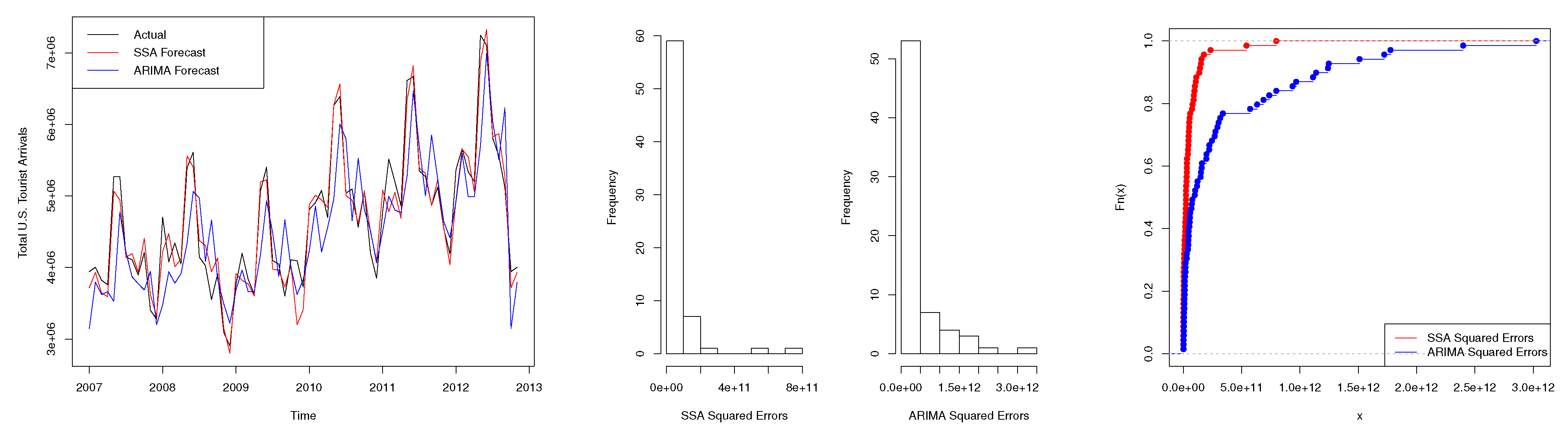
4.1. Scenario 1: Tourism Series

| Test | Two-Sided (p-Value) | One-Sided (p-Value) |
|---|---|---|
| Modified DM | <0.01 * | N/A |
| KSPA | <0.01 * | <0.01 * |
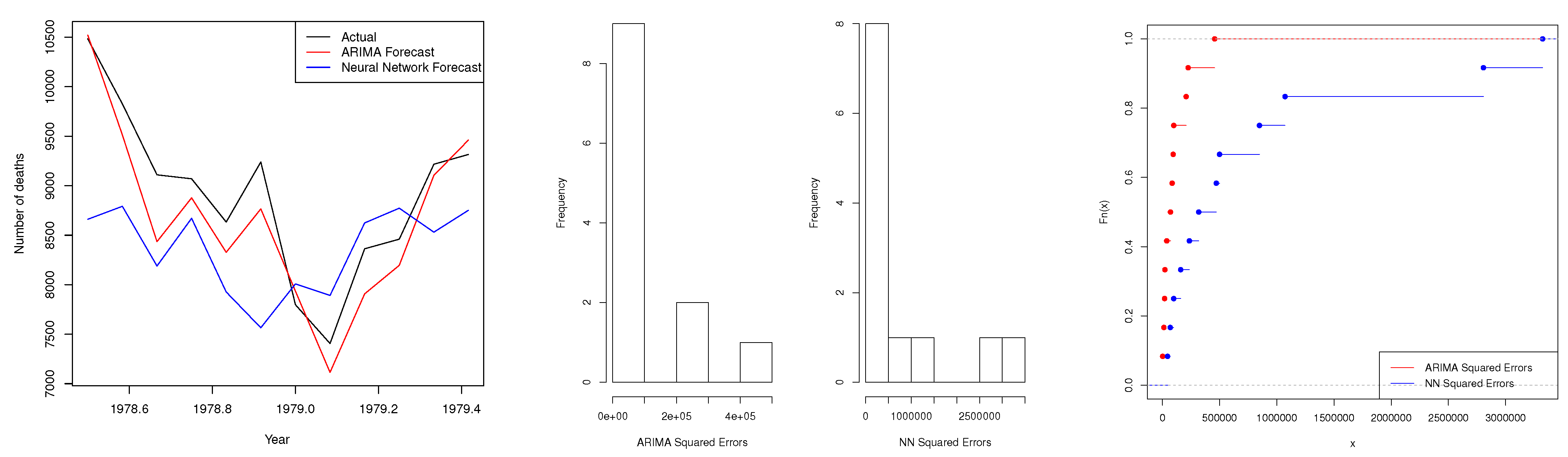
4.2. Scenario 2: Accidental Deaths Series

| Test | Two-Sided (p-Value) | One-Sided (p-Value) |
|---|---|---|
| DM | 0.04 * | N/A |
| Modified DM | N/A | N/A |
| KSPA | 0.03 * | 0.02 * |
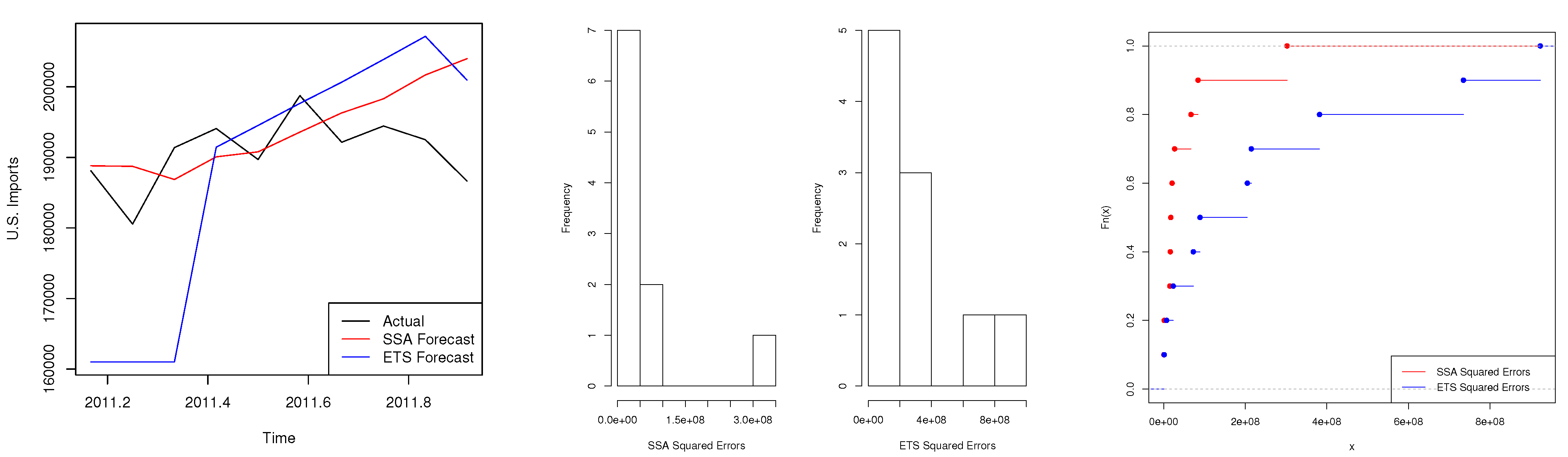
4.3. Scenario 3: Trade Series

| Test | Two-Sided (p-Value) | One-Sided (p-Value) |
|---|---|---|
| Modified DM | 0.30 | N/A |
| KSPA | 0.17 | 0.08 * |
5. Conclusions
Supplementary Materials
Supplementary File 1Acknowledgments
Author Contributions
Conflicts of Interest
Appendix: R Code for the KSPA Test
	  # Install and load the "stats" package in R.
	  install.packages("stats")
	  library(stats)
	  # Input the forecast errors from two models. Let Error1 show errors
	  from the model with the lower error based on some loss function.
	  Error1<-scan()
	  Error2<-scan()
	  # Convert the raw forecast errors into absolute values or squared values
	  depending on the loss function.
	  abs1<-abs(Error1)
	  abs2<-abs(Error2)
	  sqe1<-(Error1)^2
	  sqe2<-(Error2)^2
	  # Perform the KSPA tests for distinguishing between
	  the predictive accuracy of forecasts from the two models*.
	  # Two-sided KSPA test:
	  ks.test(abs1,abs2)
	  # One-sided KSPA test:
	  ks.test(abs1,abs2, alternative = c("greater"))
	  OPTIONAL GRAPHS FOR MORE INFORMATION
	  # Draw histograms for the forecast errors from each model.
	  par(mfrow=c(1,2))
	  hist(abs1, xlab="Model 1 Absolute Errors", main="")
	  hist(abs2, xlab="Model 2 Absolute Errors",main="")
	  # Plot the cdf of forecast errors from each model*.
	  plot(ecdf(abs1),do.points=T,col="red",xlim=range(abs1,abs2),main="")
	         plot(ecdf(abs2),do.points=T,col="blue",add=TRUE, main="")
	  legend("bottomright",legend=c("Model 1 Absolute Errors","Model 2
	  Absolute Errors"), lty=1, col=c("red","blue"))
	  #NOTE: *Replace abs1 and abs2 with sqe1 and sqe2 as appropriate.
References
- G. Elliot, and A. Timmermann. Handbook of Economic Forecasting. Amsterdam, Netherlands: North Holland, 2013. [Google Scholar]
- D.I. Harvey, S.J. Leybourne, and P. Newbold. “Testing the equality of prediction mean squared errors.” Int. J. Forecast. 13 (1997): 281–291. [Google Scholar] [CrossRef]
- R. Meese, and K. Rogoff. “Was it real? The exchange rate-interest rate differential relation over the modern floating-rate period.” J. Finance 43 (1988): 933–948. [Google Scholar]
- L.J. Christiano. “p*: Not the inflation forecasters holy grail.” Fed. Reserve Bank Minneap. Q. Rev. 13 (1989): 3–18. [Google Scholar]
- F.X. Diebold, and R.S. Mariano. “Comparing predictive accuracy.” J. Bus. Econ. Stat. 13 (1995): 253–263. [Google Scholar]
- F.X. Diebold. Comparing Predictive Accuracy, Twenty Years Later: A Personal Perspective on the Use and Abuse of Diebold-Mariano Tests. Philadelphia, PA, USA: Department of Economics, University of Pennsylvania, 2013, pp. 1–22. [Google Scholar]
- P.R. Hansen. “A test for superior predictive ability.” J. Bus. Econ. Stat. 23 (2005): 365–380. [Google Scholar] [CrossRef]
- P.R. Hansen, A. Lunde, and J.M. Nason. “Model confidence set.” Econometrica 79 (2011): 453–497. [Google Scholar] [CrossRef]
- T.E. Clark, and M.W. McCracken. “In-Sample Tests of Predictive Ability: A New Approach.” J. Econom. 170 (2012): 1–14. [Google Scholar] [CrossRef]
- T.E. Clark, and M.W. McCracken. “Nested Forecast Model Comparisons: A New Approach to Testing Equal Accuracy.” J. Econom. 186 (2015): 160–177. [Google Scholar] [CrossRef]
- E. Gilleland, and G. Roux. “A new approach to testing forecast predictive accuracy.” Meteorol. Appl. 22 (2015): 534–543. [Google Scholar] [CrossRef]
- T. Gneiting, and A.E. Raftery. “Strictly Proper Scoring Rules, Prediction, and Estimation.” J. Am. Stat. Assoc. 102 (2007): 359–378. [Google Scholar] [CrossRef]
- E.S. Silva, and H. Hassani. “On the use of Singular Spectrum Analysis for Forecasting U.S. Trade before, during and after the 2008 Recession.” Int. Econ. 141 (2015): 34–49. [Google Scholar]
- H. Hassani, A. Webster, E.S. Silva, and S. Heravi. “Forecasting U.S. Tourist arrivals using optimal Singular Spectrum Analysis.” Tour. Manag. 46 (2015): 322–335. [Google Scholar]
- H. Hassani, E.S. Silva, R. Gupta, and M.K. Segnon. “Forecasting the price of gold.” Appl. Econ. 47 (2015): 4141–4152. [Google Scholar] [CrossRef]
- C.W.J. Granger, and P. Newbold. Forecasting Economic Time Series. New York, NY, USA: Academic Press, 1977. [Google Scholar]
- W.A. Morgan. “A test for significance of the difference between two variances in a sample from a normal bivariate population.” Biometrika 31 (1939): 13–19. [Google Scholar]
- H. Hassani. “A note on the sum of the sample autocorrelation function.” Phys. A Stat. Mech. Its Appl. 389 (2010): 1601–1606. [Google Scholar] [CrossRef]
- H. Hassani, N. Leonenko, and K. Patterson. “The sample autocorrelation function and the detection of Long-Memory processes.” Phys. A Stat. Mech. Its Appl. 391 (2012): 6367–6379. [Google Scholar] [CrossRef]
- A.N. Kolmogorov. “Sulla determinazione emperica delle leggi di probabilita.” Giornale dell’ Istituto Italiano degli Attuari 4 (1933): 1–11. [Google Scholar]
- H. Hassani, S. Heravi, and A. Zhigljavsky. “Forecasting European industrial production with Singular Spectrum Analysis.” Int. J. Forecast. 25 (2009): 103–118. [Google Scholar] [CrossRef]
- H. Hassani, S. Heravi, and A. Zhigljavsky. “Forecasting UK industrial production with multivariate Singular Spectrum Analysis.” J. Forecast. 32 (2013): 395–408. [Google Scholar] [CrossRef]
- L. Horváth, P. Kokoszka, and R. Zitikis. “Testing for stochastic dominance using the weighted McFadden-type statistic.” J. Econom. 133 (2006): 191–205. [Google Scholar] [CrossRef]
- D. McFadden. “Testing for Stochastic Dominance.” In Studies in the Economics of Uncertainty: In Honor of Josef Hadar. Edited by T.B. Fomby and T.K. Seo. New York, NY, USA; Berlin, Geramny; London, UK; Tokyo, Japan: Springer, 1989. [Google Scholar]
- G.F. Barrett, and S.G. Donald. “Consistent tests for stochastic dominance.” Econometrica 71 (2003): 71–104. [Google Scholar] [CrossRef]
- M.H. DeGroot, and M.J. Schervish. Probability and Statistics, 4th ed. Boston, MA, US: Addison-Wesley, 2012. [Google Scholar]
- G. Marsaglia, W.W. Tsang, and J. Wang. “Evaluating Kolmogorov’s distribution.” J. Stat. Softw. 8 (2003): 1–4. [Google Scholar]
- Z.W. Birnbaum, and F.H. Tingey. “One-sided confidence contours for probability distribution functions.” Ann. Math. Stat. 22 (1951): 592–596. [Google Scholar] [CrossRef]
- R. Simard, and P. L’Ecuyer. “Computing the Two-Sided Kolmogorov-Smirnov Distribution.” J. Stat. Softw. 39 (2011): 1–18. [Google Scholar]
- P.J. Brockwell, and R.A. Davis. Introduction to Time Series and Forecasting. New York, NY, US: Springer, 2002. [Google Scholar]
- H. Hassani. “Singular Spectrum Analysis: Methodology and Comparison.” J. Data Sci. 5 (2007): 239–257. [Google Scholar]
- H. Hassani, R. Mahmoudvand, H.N. Omer, and E.S. Silva. “A Preliminary Investigation into the Effect of Outlier(s) on Singular Spectrum Analysis.” Fluct. Noise Lett. 13 (2014). [Google Scholar] [CrossRef]
- S. Sanei, and H. Hassani. Singular Spectrum Analysis of Biomedical Signals. Boca Raton, FL, US: CRC Press, 2015. [Google Scholar]
- 2See [14] for the calculation and interpretation of the RRMSE criterion.
- 3Data source: http://travel.trade.gov/research/monthly/arrivals/.
- 4Data source: http://www.bea.gov/international/index.htm.
© 2015 by the authors; licensee MDPI, Basel, Switzerland. This article is an open access article distributed under the terms and conditions of the Creative Commons Attribution license ( http://creativecommons.org/licenses/by/4.0/).
Share and Cite
Hassani, H.; Silva, E.S. A Kolmogorov-Smirnov Based Test for Comparing the Predictive Accuracy of Two Sets of Forecasts. Econometrics 2015, 3, 590-609. https://0-doi-org.brum.beds.ac.uk/10.3390/econometrics3030590
Hassani H, Silva ES. A Kolmogorov-Smirnov Based Test for Comparing the Predictive Accuracy of Two Sets of Forecasts. Econometrics. 2015; 3(3):590-609. https://0-doi-org.brum.beds.ac.uk/10.3390/econometrics3030590
Chicago/Turabian StyleHassani, Hossein, and Emmanuel Sirimal Silva. 2015. "A Kolmogorov-Smirnov Based Test for Comparing the Predictive Accuracy of Two Sets of Forecasts" Econometrics 3, no. 3: 590-609. https://0-doi-org.brum.beds.ac.uk/10.3390/econometrics3030590