
Bayesian Analysis of Bubbles in Asset Prices

1
Finance Department, ESSEC Business School, Paris-Singapore, Cergy-Pontoise 95021, CEDEX, France
2
School of Economics and Lee Kong Chian School of Business, Singapore Management University, 90 Stamford Road, Singapore 178903, Singapore
*
Author to whom correspondence should be addressed.
Econometrics 2017, 5(4), 47; https://0-doi-org.brum.beds.ac.uk/10.3390/econometrics5040047
Submission received: 14 July 2017
/
Revised: 11 September 2017
/
Accepted: 11 September 2017
/
Published: 23 October 2017
(This article belongs to the Special Issue Celebrated Econometricians: Peter Phillips)
Abstract
:We develop a new model where the dynamic structure of the asset price, after the fundamental value is removed, is subject to two different regimes. One regime reflects the normal period where the asset price divided by the dividend is assumed to follow a mean-reverting process around a stochastic long run mean. The second regime reflects the bubble period with explosive behavior. Stochastic switches between two regimes and non-constant probabilities of exit from the bubble regime are both allowed. A Bayesian learning approach is employed to jointly estimate the latent states and the model parameters in real time. An important feature of our Bayesian method is that we are able to deal with parameter uncertainty and at the same time, to learn about the states and the parameters sequentially, allowing for real time model analysis. This feature is particularly useful for market surveillance. Analysis using simulated data reveals that our method has good power properties for detecting bubbles. Empirical analysis using price-dividend ratios of S&P500 highlights the advantages of our method.
JEL Classification:
C11; C13; C32; G121. Introduction
The recent global financial crisis and the European debt crisis have prompted economists and regulators to work arduously to find ways to avoid the next crisis. From a historical perspective, Ahamed (2009) argues that financial crises are often preceded by an asset market bubble.1 Well-known bubble episodes include the Dutch tulip mania in the 17th century, the British South Sea bubble at the beginning of the 18th century, the Railway mania in the 1840s, the Roaring Twenties stock-market bubble, the Dot-com bubble at the end of the 1990s, and the US housing bubbles lasting until 2006. Bubbles are generally considered harmful to economies and the welfare of society and are thought to lead to the misallocation of resources. For example, Caballero et al. (2008) argues that the burst of an asset price bubble can lead to recession in the real economy. Consequently, approaches have been tried to detect the presence and the burst of financial bubbles and to estimate the bubble origination and collapsing dates.
Broadly speaking there are two alternative models in the bubble literature. Both are motivated from the following no-arbitrage condition:
where is the asset price (such as stock price) at time t, is the cash flow (such as dividend) received between and t due to the ownership of the asset, and R is the discount rate (). By forward substitutions, we obtains the following decomposition of the asset price
where is a “fundamental” component and is a bubble component which satisfies
Unless , the bubble process is a submartingale. In an autoregressive (AR) representation, with being an explosive AR root and .
In the bubble literature two alternative approaches co-exist. The first approach employs regime switching models while the other one is based on various structural break models. This latter approach has been advocated by Peter Phillips and his co-authors in recent years; see Phillips et al. (2011), Phillips and Yu (2011) or Phillips et al. 2015a, 2015b, PSY hereafter) and attracted a great deal of attention from policy makers.
Regime switching models have a long history in economics, dating back to Godfeld and Quandt (1973) and Hamilton (1989). Evans (1991) model may be regarded as a regime switching model with two regimes. One regime corresponds to bubble expansion modelled by an explosive AR model whereas the other regime corresponds to bubble collapse. This collapse is sudden, takes place within a single period and is determined by an independent Bernoulli trial. After the bubble has collapsed, a new bubble starts emerging. Another regime switching model was proposed by Funke et al. (1994) and Hall et al. (1999). In this model, two regimes have been used: one regime has a unit root and the market is efficient, whereas the other regime has a bubble and hence has an explosive root. More recently, Shi (2013) extends the model in Hall et al. (1999) to allow for heteroskedasticity. Shi and Song (2015) proposed to use an infinite hidden Markov model, which allows for an infinite number of regimes to detect, date stamp and estimate speculative bubbles.
Structural break models have been extensively used to distinguish stationary models from unit root models; see for example, Kim (2000) and Busetti and Taylor (2004). Recently, Phillips et al. (2011), Phillips and Yu (2011), Homm and Breitung (2012), and PSY extend some of the methods to distinguish explosive models from unit root models. In all the models considered, the change point is not stochastic.
Regarding statistical inference on the presence of bubbles and the date-stamping of bubble origination and termination, several methods have been proposed. The first method is based on the full sample maximum likelihood (ML) method. This includes Funke et al. (1994) and Hall et al. (1999) in the context of regime switching models. When the model is correctly specified, the ML estimator (MLE) is efficient. Probabilistic inference about the unobserved regimes can be based on the Hamilton filter by calculating either the filtered probability or the smoothed probability. These probabilities naturally depend on the unknown parameters. To estimate the probabilities, the unknown parameters are replaced by the MLE obtained from the full sample. Consequently, the inferential approach does not allow for real time analysis as there is no sequential learning about the parameters. This feature of lack of real time analysis is shared by some MCMC algorithms in the literature such as the one in Shi and Song (2015).
The second method is based on recursive techniques. For example, Phillips et al. (2011) and Phillips and Yu (2011) suggest implementing the right-tailed ADF test repeatedly on a forward expanding sample sequence. To effectively deal with episodes with multiple bubbles, PSY (2015a) and PSY (2015b) vary both the initial point and the ending point of the sample in each recursive regression. Homm and Breitung (2012) modifies various recursive methods for the purpose of bubble detection and date-stamping of bubble origination and termination. Apart from its ease of implementation, a nice feature of the recursive method is that it provides real time estimate of the bubble state. In practice, however, it is possible that the chosen minimum window size is larger than the actual bubble duration. Moreover, for the test statistic to rise above the critical value, a long enough period and a strong enough signal from the explosive regime are needed. Not surprisingly, in finite samples, the method may be late to identify the bubble origination and collapsing dates.
In this paper, we make several contributions to the empirical asset pricing literature. First, we propose a two-state regime switching model of bubbles that generalizes the existing literature. The underlying series that we model is a price divided by a proxy of its fundamental component. A typical example would be a stock price divided by its dividend. The rationale is that in rational asset pricing models the asset price is the discounted present value of some fundamental hence there may be a common trend between asset prices and fundamentals. However, this common trend is canceled if we divide prices with the fundamental, resulting in a stationary series. The variation in this ratio may either reflect some stationary non-fundamental factors, some unobserved fundamentals (i.e., noise in the proxy for the fundamental) or low-frequency cyclical movements in the discount rates suggested in the recent finance literature (Cochrane 2011). Here we are not trying to differentiate between these explanations, in our normal state we simply assume mean-reverting dynamics around some long-run mean. In addition, to allow for smooth permanent structural changes in asset markets, we allow this long-run mean itself to follow a random walk process. Evidently when the variance of this latter is set to zero, smooth structural change is excluded. For the duration of this normal regime we assume a standard exponential distribution that implies Markovianity of the regime changes. In addition to this normal state, we add a second state corresponding to bubble periods where the AR coefficient of the valuation ratio is larger than one. Here we depart from the extant regime-switching literature and allow for non-constant hazard rates of exit from the bubble regime corresponding to Weibull-distributed durations. Throughout we assume normally distributed innovations and allow conditional heteroskedasticity through an independent Markov switching process.
Our second contribution is to implement a Bayesian learning approach for sequential joint statistical inference over latent states, model parameters, and model comparison. There are several appealing features of this new inferential method for bubble detection. Firstly, based on the regime switching method, we can avoid the need to specify the minimum duration of each regime, including the bubble regime. In PSY, the minimum duration is set to the minimum window size of regression. In the case when the minimum window size has to be specified, if the minimum window size is larger than the minimum duration of a regime, the identification of a regime will be biased. Consequently, it is reasonable to believe that our model can identify the change points more effectively and more quickly when there are quick regime shifts. Secondly, the change points are endogenously determined. Thirdly, we are able to deal with parameter uncertainty as well as learning about the states and the parameters sequentially, allowing for real time model analysis. This feature is particularly useful for market surveillance, as argued in PSY (2015a). Fourthly, our approach enables exact finite sample inference about the parameter as well as latent states and hence avoids the derivation of asymptotic distributions. As shown in PSY, the asymptotic properties can be very difficult to obtain in general and this is especially true for the estimator of the change point.2
To check the reliability of the proposed method for the model, we conduct a Monte Carlo study. The Monte Carlo results show that the method is reliable both for the estimation of parameters and more importantly for detecting bubbles. Comparing its performance to PSY we find that our Bayesian learning algorithm reacts faster and has better power to detect bubbles. In further robustness tests we find that our method is robust both to the presence of non-normal innovations and of the leverage effect in the data generating process. We also apply our method to real data, i.e., monthly S&P 500 price-dividend ratio between 1871 and 2012, as PSY did. Our empirical estimates of the timing of bubbles are broadly similar to the empirical results obtained by PSY (2015a) based on a recursive frequentist method. However, our procedure flags more bubble episodes than PSY and differentiates between bubble periods and normal periods more often. Furthermore, in line with our simulation evidence, we find that a decision maker who is averse to erroneously declaring a regime change will identify substantially fewer and longer bubble periods.
2. Econometric Model and Estimation Method
2.1. The Present Value Model and PSY’s Method
Let , , , , , with being the average log dividend-price ratio, and . A log-linear approximation of (1)–(3) yields the following present value model:
See Campbell and Shiller (1988) and Lee and Phillips (2016) for further details about the log-linearization. Equation (6) implies the following process
From (5), we get
If is an I(1) process, (8) implies that is also I(1) and that and are cointegrated with the cointegrating vector . In addition, if there is no bubble, Equation (4) suggests that , and hence that and are cointegrated. If there are bubbles which manifest with an explosive behavior in according to (7), will also be explosive too and so is , the log price-dividend ratio. This is the reason why the behavior of the price-dividend ratio has been studied in the empirical literature.
To test for bubbles, the PSY procedure relies on repeated calculations of the t-statistic in autoregression in a recursive manner where the end point (fraction) of each sample takes a value between to 1 and the starting point (fraction) of the sample takes a value between 0 to with (fraction) being the smallest sample window. Let T be the size of the full sample. So is the minimum window size in the calculations. PSY (2015a) proposed the GSADF statistic to be the largest ADF t-statistic in the double recursion over all possible combinations of and , namely
where is the ADF t-statistic based on the sample from to . PSY (2015a) derived the asymptotic distribution of when the null hypothesis is a unit root process, from which the right-tailed critical values can be obtained. The intuition why the test is reasonable is that if there is a subsample of data corresponds to an explosive bubble period, the ADF t-statistic calculated from this subsample should take a large value. The proposed test is a recursive way to find such a subsample and the corresponding ADF t-statistic.
After bubbles have been detected, the origination date and the conclusion date of each bubble can be estimated by
where
and is the critical value of the sup ADF statistic based on observations. The intuition for the two estimators is that, is the first time when the evidence of explosive behavior is found while is, given an explosive subsample of data has been found, the first time when the evidence of explosive behavior disappears. PSY studied the consistency properties of the two estimators when data are generated from the following AR model with four structural breaks,
In Model (11), there are two periods of mildly explosive bubbles in , the price-dividend ratio, where with and , , , , , for , , with , dates the origination of the ith bubble and dates its termination. Clearly if is too large such that the minimum window size is larger than the minimum bubble duration, the performance of both the bubble test and the dating estimators will be adversely affected.
2.2. Model and Inferential Task
Following the literature, we also model the price-dividend ratio, denoted by throughout the rest of the paper. We assume the presence of two regimes determining the autoregressive behavior of the series, with the normal regime, the bubble regime. The distribution of the duration of the normal regime is exponential with parameter . That is, if the duration of the normal spell is denoted by , then . As our focus is on the bubble regime, we assume that the bubble duration, , follows the more flexible Weibull distribution with parameters , giving rise to the survival probability
The expected value of the bubble spell is and we reparameterize the model and define our prior over instead of . The shape parameter determines whether the hazard rate of exit is constant, increasing or decreasing.
The process in each regime follows
In the normal state (12), follows a mean-reverting process around the stochastic mean , where the speed of mean-reversion is . To allow for gradual parameter change in the long-run mean, Equation (13) posits that follows a random walk whose variability is determined by . Obviously, when , we are back to a constant mean reversion model. In the state with an explosive root (14), we claim that there is a bubble in the asset price. This is because is an asset price with the fundamental value removed. As a result, the presence of an explosive root implies the presence of bubble according to the present value model; see, for example, Diba and Grossman (1988). Following the suggestion of Phillips et al. (2011), we do not use an intercept in the explosive state for otherwise the intercept would dominate the autoregressive term asymptotically which is not empirically realistic.3
To address the concern of Shi (2013) about the sensitivity of bubble identification to the presence of heteroskedasticity, we allow to follow an independent 2-regime Markov switching process, with diagonal probabilities . In the first (low) regime the value of volatility is while in the second (high) regime, where . The transition matrix for volatility is
The fixed parameter vector describing the dynamics of the system has 10 unknown parameters .
To monitor bubbles in real time, the user of the model needs to evaluate the probability of being in a bubble (or normal) regime at time t, given information available by time t. Even if he knows the fixed parameters , inference over the regimes, i.e., obtaining
is not easy as the filter is not analytically available for the model. However, in what follows we describe a very efficient sequential Monte Carlo technique (a particle filter) to numerically approximate the filtering distributions.
2.3. Discrete Particle Filter
The theoretical quantity that the filtering algorithm targets is the sequence of filtering distributions of the state-space system where is the time elapsed since the last regime change. Throughout this section we assume a known parameter vector and, to simplify notation, we suppress dependence on it. The crucial thing to realize is that conditional on the path of the discrete latent states the system is a linear Gaussian state space model, and hence the continuous state variable can be marginalized out analytically using Kalman filtering recursions. Let us denote the two filtering moments of (conditional on discrete latent variables) by , and hence the joint filtering density to track becomes . Given that the state space that we need to filter numerically is discrete, we can employ the discrete particle filter (DPF) of Fearnhead (1998) where all successor states are generated avoiding the use of a proposal distribution. Let us assume that at we have N equal-weighted particles with weights representing the filtering distribution. We have the following recursion to arrive to the filtering distribution at the next time instant t.
Branching out: To move the hidden state particles forward, one needs to attach to the existing particles to characterize . Instead of some random proposal over the new states the DPF proposes to create all possible successor states from each existing particles. In our case we have possible successor particles for each ancestor corresponding to all possible configurations of . This results in particles of the form with attached weights
Attaching new information and computing the likelihood: Next, the particles are reweighted to include the effect of the new observation . The theoretical relationship between the predictive distribution and the filtering one is
This can be implemented in the algorithm by reweighting to arrive to the filtering weights . The estimate of the marginal likelihood of can be computed as
Resampling: Clearly, repeating the previous steps through multiple observations would lead to an exponential growth in the number of discrete states to be maintained. Hence it is crucial to include a resampling step where N particles are sampled out of the existing one with probability proportional to the normalized weights . This results in an N-sample, with equal weights . The last step is to update the hidden variables which are simply deterministic functions of their past values, the new state variables and of the observation .
The empirical distribution of the particle cloud converges to the true filtering density under weak conditions and it can be used to approximate any filtering quantity of interest. For example the filtered bubble probability can be approximated as:
2.4. Parameter Learning Algorithm
In practice, we do not know . A common practice in the regime switching literature is to replace by the ML estimates or the Bayesian estimates obtained from the full sample, ignoring the parameter uncertainty. Since the estimates of are constructed from the full data sample, such an analysis is not in real time. To carry out a real time analysis, the model parameters also need to be sequentially updated as new data arrive. Furthermore, ignoring parameter uncertainty can lead to an overestimation of our ability to detect regimes in real time, especially for more complex models.
To tackle these issues we turn to sequential Bayesian techniques that allow us to sample from the posterior probability of the fixed parameters . As an example, assume that we have a weighted sample with normalized weights whose empirical distribution approximates . Further, assume that for each , we have N state particles approximating obtained by running a DPF at . Then the posterior probabilities that take parameter uncertainty into account can be computed as
Bayesian methods enable us to conduct the exact finite sample inference of the parameters as well as latent states. In contrast, the derivation of asymptotic properties of classical estimators can be very difficult for this class of models due to the presence of explosiveness. This difficulty is especially true for the estimator of the change point; see, for example, PSY (2015b).
Sequential analysis of state-space models under parameter uncertainty is of interest in many settings. Since one of our primary interests here is real time analysis of regime detection, parameter learning is needed. To sequentially learn over the parameters, we turn to the marginalized resample-move approach of Fulop and Li (2013) and Chopin et al. (2013). For completeness, we provide a brief overview of the method in this subsection. We need a method to sequentially sample from the sequence of posteriors
where is the prior over the fixed parameters and for notational convenience we suppress the dependence on the initial hidden state. While the individual conditional likelihood cannot be obtained in closed form, Fulop and Li (2013) and Chopin et al. (2013) employ instead the approximate likelihood obtained from particle filters. In particular, instead of the target in (15) they propose to work with the extended target
where the likelihood estimates (denoted as in the previous section) are obtained by running a particle filter with N particles for any given fixed parameter , contains all the random variables created at time l by the particle filter and is the density of these random variables.
Initialization: Sample particles from the prior , and attach equal weights to each particle . The resulting cloud, is trivially distributed according to . For each initialize a particle filter with N state particles and denote the random variables created by .
Recursion and reweighting: Assume that a weighted sample, , has been obtained that represents . Furthermore, for each we maintain a particle filter with N state particles with attached random variables and the likelihood estimates up to , . Now the task is to include the new observation into the information set and obtain a representation of the next posterior, . The sequential resample-move algorithm uses importance sampling for this task and the intuition that the posterior at is typically quite close to the posterior at t. Hence, the sample from the former will provide a good proposal distribution for the latter. Then the location of the particles is inherited from the previous cloud: . However, the importance weights will change to account for the difference between the target and the proposal leading to new un-normalized weights
The incremental weights are obtained by running the particle filter for each on the new observation and recording the resulting likelihood estimate. The random numbers used in the particle filters need to be independent across and through time. The new normalized weights are and the particle cloud, , will represent the target .
Sample Degeneracy: If we keep repeating the reweighting steps, at some point the sample would degenerate. We measure sample diversity by the Efficient Sample Size: . Whenever the drops below some pre-specified number B, we will introduce additional algorithmic steps to improve the support of the distribution.
Resampling Step: First, to focus computational efforts on the more likely part of the sample space, we resample the particles proportional to weights to arrive to an equal-weighted sample and set weights to . Any resampling method can be used where choice probabilities are proportional to the weights. Also, notice that for each resampled , the attached dynamic states and likelihood estimates need to be resampled too. The resulting cloud is still distributed according to .
Move Step: The resampling step in itself does not enrich the support of the particle cloud. We need to boost the particle cloud in such a way that does not distort its distribution in a probabilistic sense as M goes to infinity. This can be achieved by moving each particle through a kernel that admits as an equilibrium distribution. will be a particle marginal M-H kernel from Andrieu et al. (2010):
- Propose from a proposal density: .
- Acceptance probability:
- With probability , set , otherwise keep original value.
Here, can be fitted on the cloud of particles to better approximate the target. Fulop and Li (2013) and Chopin et al. (2013) show that this algorithm actually delivers exact inference over the sequence of joint filtering distribution of the parameters and the dynamic states.
Notice that the move step needs to browse through the full data-set as the likelihood is evaluated at each new proposal . In contrast, the reweighting step only needs the last individual likelihood . Hence the time needed for a move step keeps increasing with the sample size, while the reweighting step has a constant speed. Fortunately, as the sample becomes large the posteriors stabilize and one needs to resort to move steps less and less often. To keep the estimation error in the likelihood under control, under some mixing assumption on the state-space model the number of state particles need to increase linearly with the overall sample size. Chopin et al. (2013) show that overall the computational cost of the algorithm is of the order .
2.5. Loss Functions for Bubble-Stamping
The discrete decision a policy maker is facing at time t is whether he stamps the given period as a bubble or not. Let us denote this decision as if the period is stamped as a normal period, if it is stamped as a bubble period. Then the loss function corresponding to the decision is defined as
where is the loss from classifying a normal period as a bubble period while is the loss from classifying a bubble period as a normal period. If the policy maker is averse to quickly reversing the labels he has announced, we can let these loss functions be state-dependent. In particular, if the previous period was stamped as a normal period (), we would have and the reverse if the previous period was stamped as a bubble period. The expected losses of the policy maker based on real time information corresponding to the two decisions are
Hence, flagging the period as a bubble period is optimal if
Notice that for decision-making it is only the ratio of the loss functions denoted by that matters. If we assume that this parameter is time invariant conditional on being in a regime stamped as a normal regime, the rule is to stamp the new regime as a bubble if . By analogy, we stamp the end of a bubble spell whenever .
3. Monte Carlo Study
3.1. Priors and Parameter Restrictions
In the simulation study and the empirical study, we use the following parameter restrictions and prior distributions for the model parameters:
- This is the parameter determining the expected length of a normal regime. To reflect our a priori beliefs that the normal regime should be reasonably long lasting, we enforce the restriction . The prior distribution we use is then a truncated normal with mean and standard deviation parameters of 180 and 60 respectively.
- Determines the shape of the bubble regime distribution. Here we assume that has an increasing probability of exit from the bubble state in duration reflected in a parameter restriction . The prior distribution we use is then a normal distribution truncated from below with mean and standard deviation parameters of 1.
- : Determines the expected length of a bubble spell. Here again we restrict the parameter to focus on reasonably long-lasting bubble spells, by enforcing . Then ,the prior we use is a normal distribution truncated from below with mean and standard deviation parameters of the normal of 36 and 12 respectively.
- For both we use a uniform prior on .
- We use a normal prior truncated below at 0, with .
- Given that this is the ratio of the volatilities between the high and low-volatility states, we use the parameter restriction . Then, the prior distribution we use is a normal prior truncated below with .
- We use a normal prior truncated below at 0, with .
- Measures the mean reversion during the normal regime. The recent literature in finance points towards time-varying discount rates as the main source behind the cyclical variation in the price-dividend ratio (see for instance Cochrane (2011) for a recent overview), usually thought of as a medium-to-low frequency phenomenon. Hence we bound from below the half-life of the mean reversion at 2 years, corresponding to with monthly data. In addition to this we only assume non-explosiveness of the process in the normal regime leading to the uniform prior reflecting the parameter restriction .
- Here we use the parameter restrictions . The upper boundary is chosen to make sure that we cover all empirically relevant parameters of . Then the prior distribution we use is .
In the SMC procedure we use parameter particles with state particles in each particle filter. The resample-move step is triggered when the efficient sample size drops below . In the move-steps we use an independent mixture normal proposal. The routine has been coded in MATLAB with the particle filtering operation programmed efficiently in CUDA and run on a Kepler K20 GPU.
3.2. Monte Carlo Results
To investigate the reliability of the learning routine we design two Monte Carlo experiments. In the first experiment, we simulate 100 data sets from the proposed regime switching model, each with observations. The parameter setting, including the sample size, is similar to what we find later in the empirical study using the S&P500. The first column of Table 1 reports the parameter values used to generate the data. The second column reports the average of the full-sample posterior means and the third column the average length of the central posterior credible interval. For comparability the last column shows the prior central credible interval. The results show that the informativeness of the data varies starkly across the various parameters. First, one can see that the length of the posterior credible interval for is only a bit smaller compared to the prior analogue, mirroring limited learning about these parameters that determine the regime transition probabilities. This is a natural consequence of the small average number of regime changes in the simulated data. Not surprisingly, the average posterior means are markedly biased towards the prior means. A similar phenomenon can be observed for that controls the variability of the long-run mean of the time-series. The reason here is that changes in happen at a low frequency resulting in a small effective sample. The remaining parameters, , describe time-varying volatility and the within-regime conditional means and are much better identified from the data. The posterior means are close to the real generating values and the posterior credible intervals are a fraction of the prior ones.
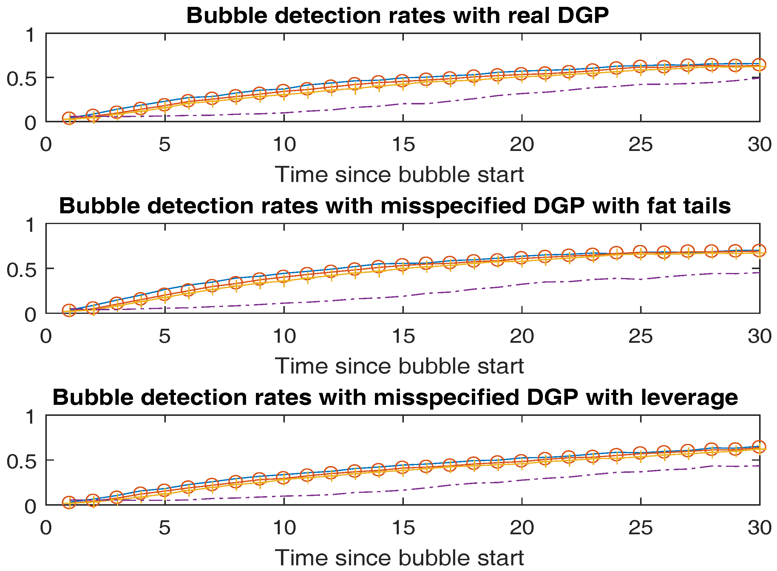
Now we turn to the ability of our model to detect explosive periods (bubbles) in the underlying time series and compare it with the real time detection algorithm in PSY. In our Bayesian algorithm we investigate several values of the date-stamping parameter . As a baseline, we look at the case of symmetric loss, i.e., . Then, we also investigate cases where the decision maker is averse to changing the stamp too quickly. Specifically, we look at and . For PSY, we follow Yiu et al. (2013) and declare a switch to a bubble stamp whenever the backward sup ADF (BSADF) test statistic surpasses where is the critical value of the test statistic obtained by Monte Carlo simulation. Further, we stamp the end of the bubble when the statistic drops below . Note that both algorithms are implementable using only data available in real time. In the upper panel of Figure 1 we plot with solid lines the detection rates of our Bayesian learning algorithm as a function of bubble duration, where the flat line corresponds to , the line with circles to and the line with plus signs to . The dashed line reports the detection rates from using the BSADF statistic as in PSY. All results are averaged across 100 data sets using the true DGP to simulate the data. One can see that our Bayesian methodology seems to react faster with better detection rates when only a few periods has elapsed since the start of the bubble. The power of the two algorithms seems to get closer as the length of bubble becomes large. Importantly, the detection capability of the test does not seem to deteriorate much with an increase in the bubble stamping parameter . Let us note that the size of the Bayesian test (periods flagged as bubble that are in fact not bubbles) is around while for PSY it is . There are at least two usual caveats with the use of relatively richly parameterized nonlinear models like our regime-switching one in time-series. The first is the concern about parameter uncertainty while the second is about the robustness of the results to the exact model specification. As mentioned earlier, our Bayesian learning approach deals with the first of these as it fully takes parameter uncertainty into account.
However, one may still wonder about the extent to which these detection results are conditional on the model being exact. To try to address this concern, we also investigate the behavior of our procedure under two misspecified DGP’s each formalizing a well-known stylized feature of asset return that is ignored in our model. First, in the middle panel of Figure 1 we investigate the detection capability of our method and that of PSY in a setting where the data innovations follow a fat-tailed student-t distribution with 4 degrees of freedom instead of the normal postulated by our regime switching model. Second, we allow for a leverage effect by allowing the probability of jumping to the high-volatility regime to be correlated with the innovations in . In particular, we draw from a bivariate standard normal distribution with correlation coefficient , and use the first coordinate as the innovation in and define the regime switching event in the subsequent period from the low volatility regime to the high volatility regime as where is the inverse normal cumulative density function and is the second coordinate of the normal noise. By this construction the probability of jumping to the high volatility regime is higher following a decrease in the asset price, giving rise to the leverage effect. Both panels with misspecified DGP’s closely mirror the ones in the upper panel showing the robustness of our method to the presence of fat-tailed innovations.
To gain further insight into the behavior of identified bubbles by the alternative bubble indicators, Table 2 reports some summary statistics of identified bubbles. It shows the number of identified bubble episodes, the proportion of the identified bubble periods and the average bubble duration, both for PSY and the regime switching model with different value of . The first and third columns show that both PSY and the regime switching model with (no aversion to regime change) indicate more frequent but shorter bubbles compared to . Hence, allowing for a “regime-change-averse” loss function for the decision maker provides a principled way to flag fewer and longer bubbles in the regime-switching framework. Furthermore, the second column indicates that the proportion of periods labeled as bubble is much less variable across the different methods. Hence, these results are not simply the result of using a more aggressive test procedure.
4. Empirical Study
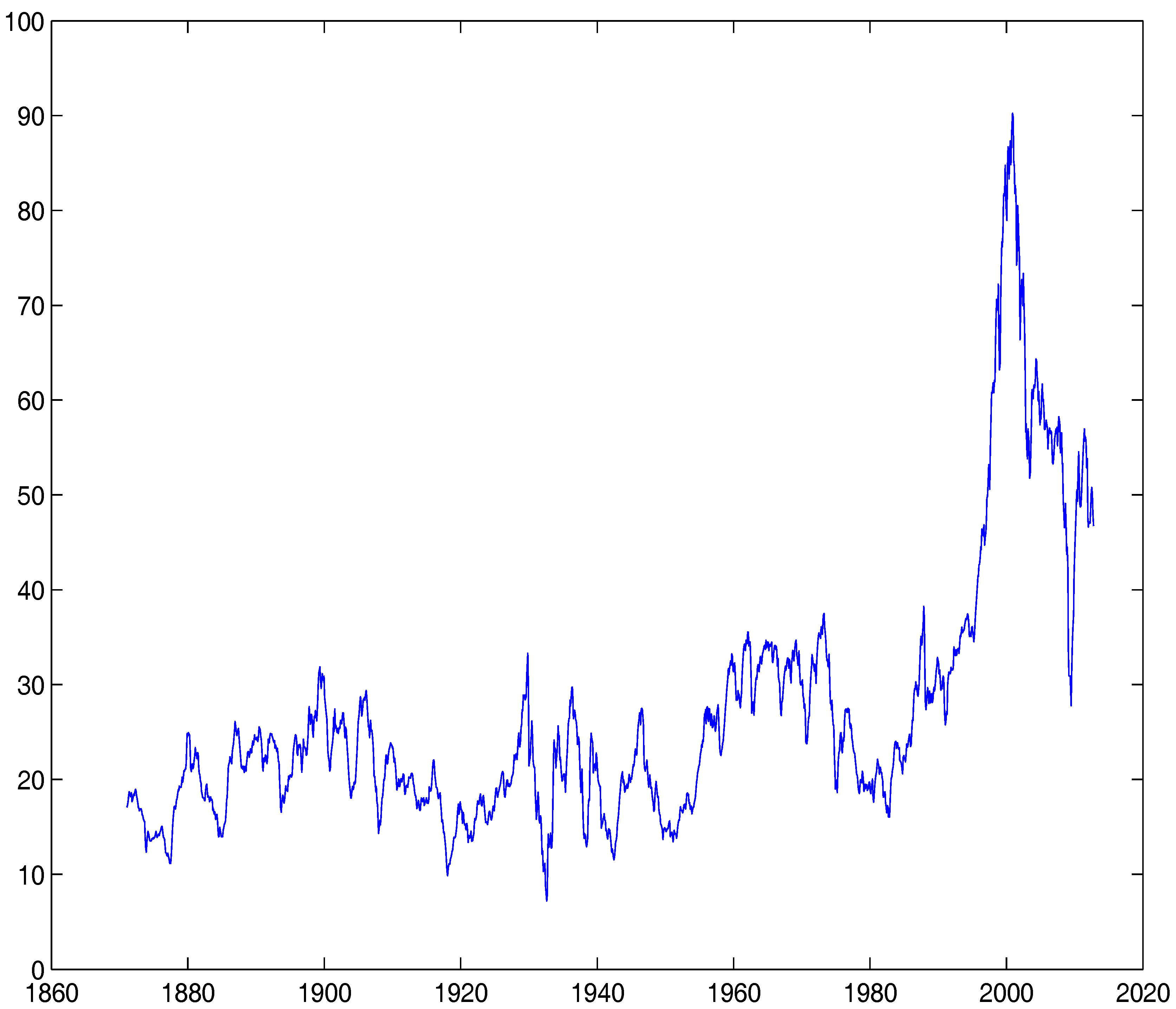
In the empirical study, we confront the proposed model with a well-known time series. We fit the model to the monthly real S&P500 series and dividend series as in PSY (2015a). The data series is from January 1871 to June 2012, resulting in 1698 observations and downloadable from Professor Robert Shiller’s website.4 As in PSY, we investigate the series of the price-dividend ratio, plotted in Figure 2. The choice of the data over a long time span reflects our objective to capture as many stock market phases as possible. In the meantime, the use of the same data as in PSY allows us to compare our estimates with those of PSY.
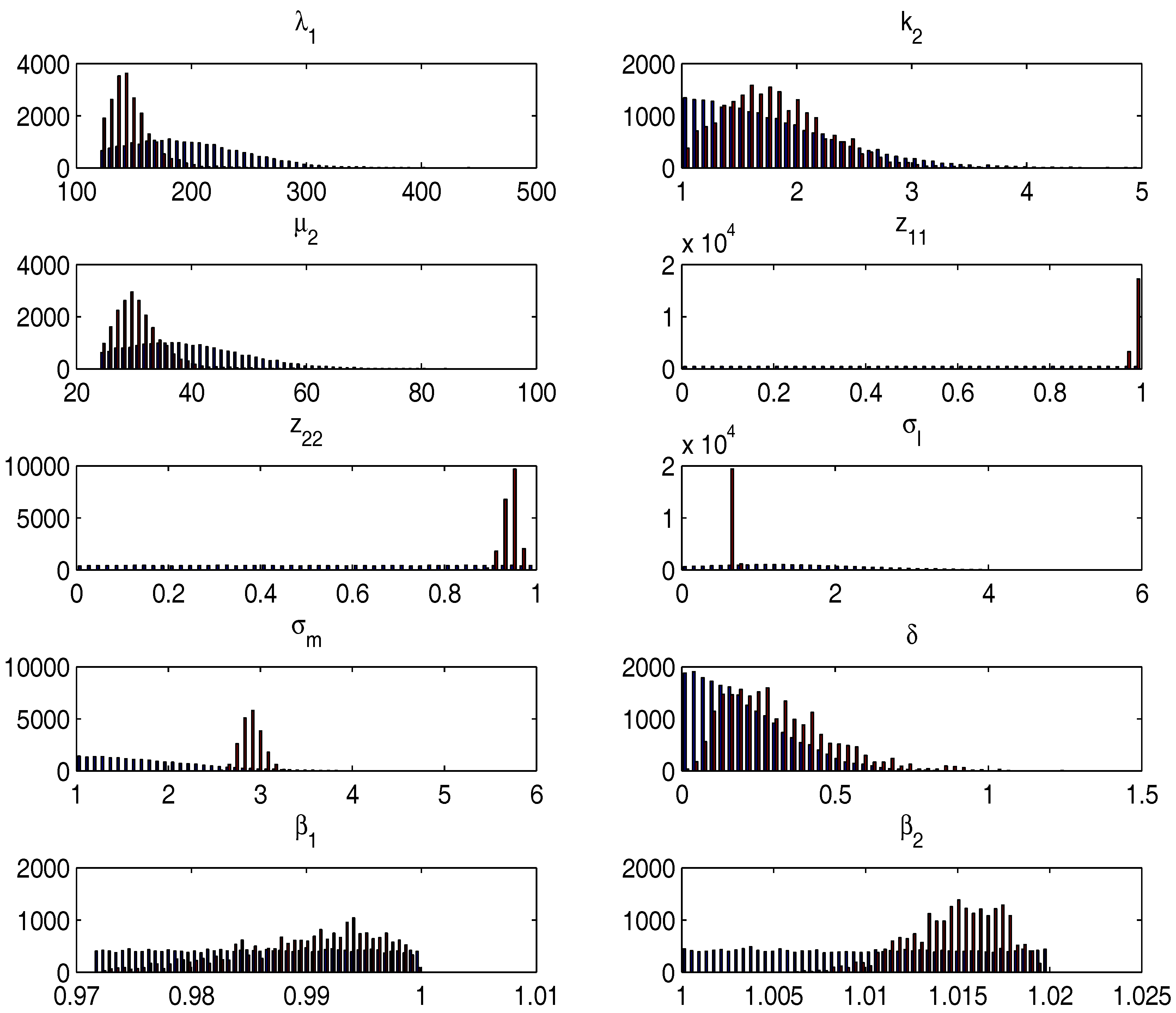
Table 3 presents the full sample posterior estimates obtained from our learning routine and Figure 3 shows the histograms of the priors (in red) alongside the full-sample posteriors (in blue). We can observe that while there is a large amount of uncertainty remaining about the parameters driving the regime changes, the data does tell us something about these parameters. First, the posteriors of both and put relatively more weight onto lower values, suggesting somewhat more frequent regime changes compared to our priors. Second, the posterior over the shape parameter of the bubble duration seems to have a density separated away from 1 providing evidence against a simple exponential bubble duration distribution (case of ). This evidence points towards an increasing hazard function of exit from the bubble state, i.e., the probability of a crash tends to increase as bubbles mature. This is in contrast to a standard homogenous continuous time Markov-Switching model that gives rise to exponentially distributed durations. Further, the presence of stochastic volatility is clear in the data. The volatility in the high volatility regime is almost three time as large as that in the low volatility regime but is markedly less persistent. As in the Monte Carlo simulations, the data does not reveal too much about , the volatility of the long-run mean, but the posterior seems separated from zero. In contrast, the mean-reversion coefficient in the normal regime seems well identified with a mode that is close to but separate from unity and a posterior mean of . To translate this parameter to a more intuitive scale, we compute the posterior mean of the half-life of the process during the normal regime. If , are the posterior draws of the parameter, the posterior mean half-life is computed as . In our data set this results in an estimate of , i.e., years. Last, the autoregressive coefficient during explosive regimes is tightly identified and symmetrically distributed around a posterior mean estimate of .
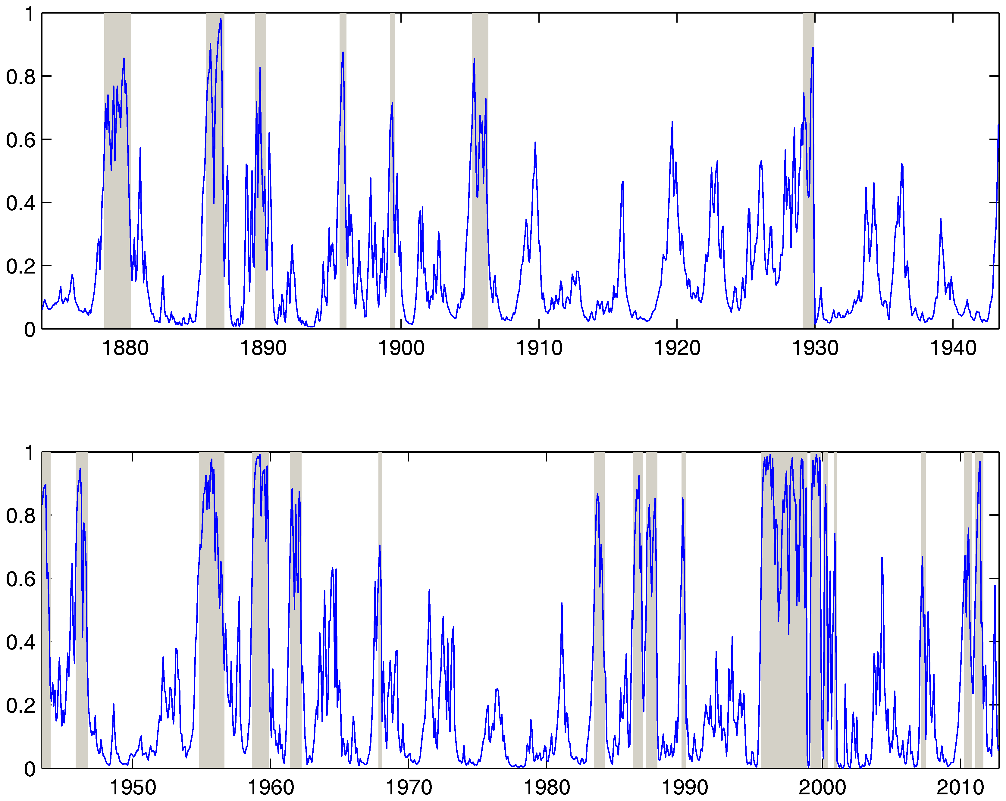
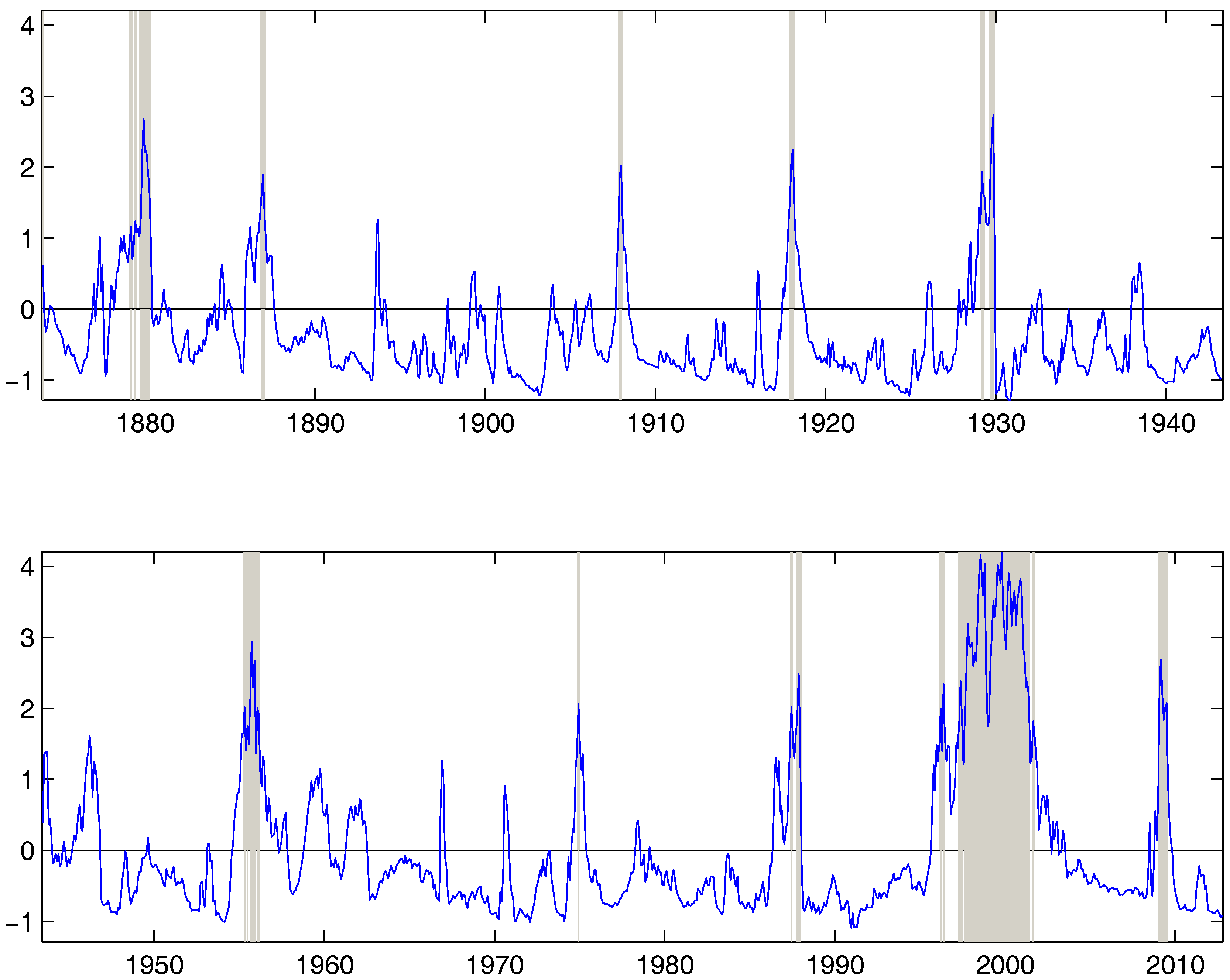
Our main object of interest is not the parameter estimates per se but the ability to detect bubbles in real time using the filtered bubble probabilities. Table 4 reports some summary statistics on bubble-stamping both from PSY (2015a) (row 1) and from our algorithm with different values of . The first thing to note is that in accordance with the simulation results, both PSY (2015a) and the regime switching model with seems to detect lots of short bubbles with the average bubble spell around 4 months in both cases. Further, increasing the date stamping parameter to seems to lead to an increase in the average length of the detected bubble spells while decreasing the number of bubble periods. Overall, allowing for aversion to change in the bubble stamps leads to more intuitive results at least for this data set. Second, the results are not too different across and . Hence, the results seem reasonably robust to the exact choice of the loss function. Last, the regime switching labels more periods as bubbles compared to PSY. Figure 4 shows the results from a real time bubble classifier with together with the filtered bubble regime probabilities. Here we label a given month a bubble (shaded in grey) if the bubble regime has the highest filtered probability. For comparison, we also implement the real time bubble indicator using the BSADF statistics from PSY in Figure 5. It is reassuring to observe that there are quite a few periods where the incidence of bubbles is preponderant according to both methods. In particular, around 1880, the years before 1920, before the great depression in 1929, the internet bubble before 2000 and last, the rebound after the recent 2008 financial crisis.
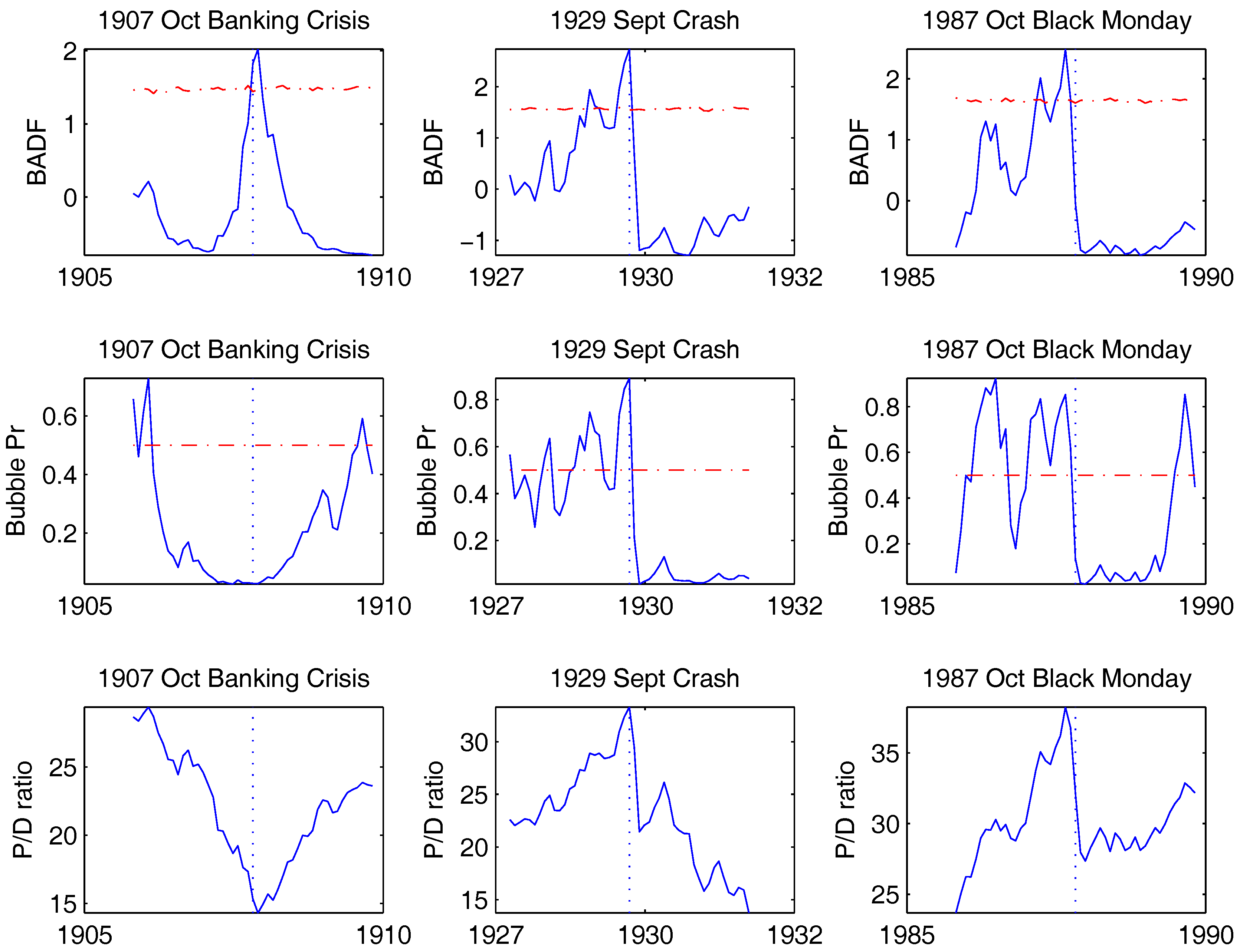
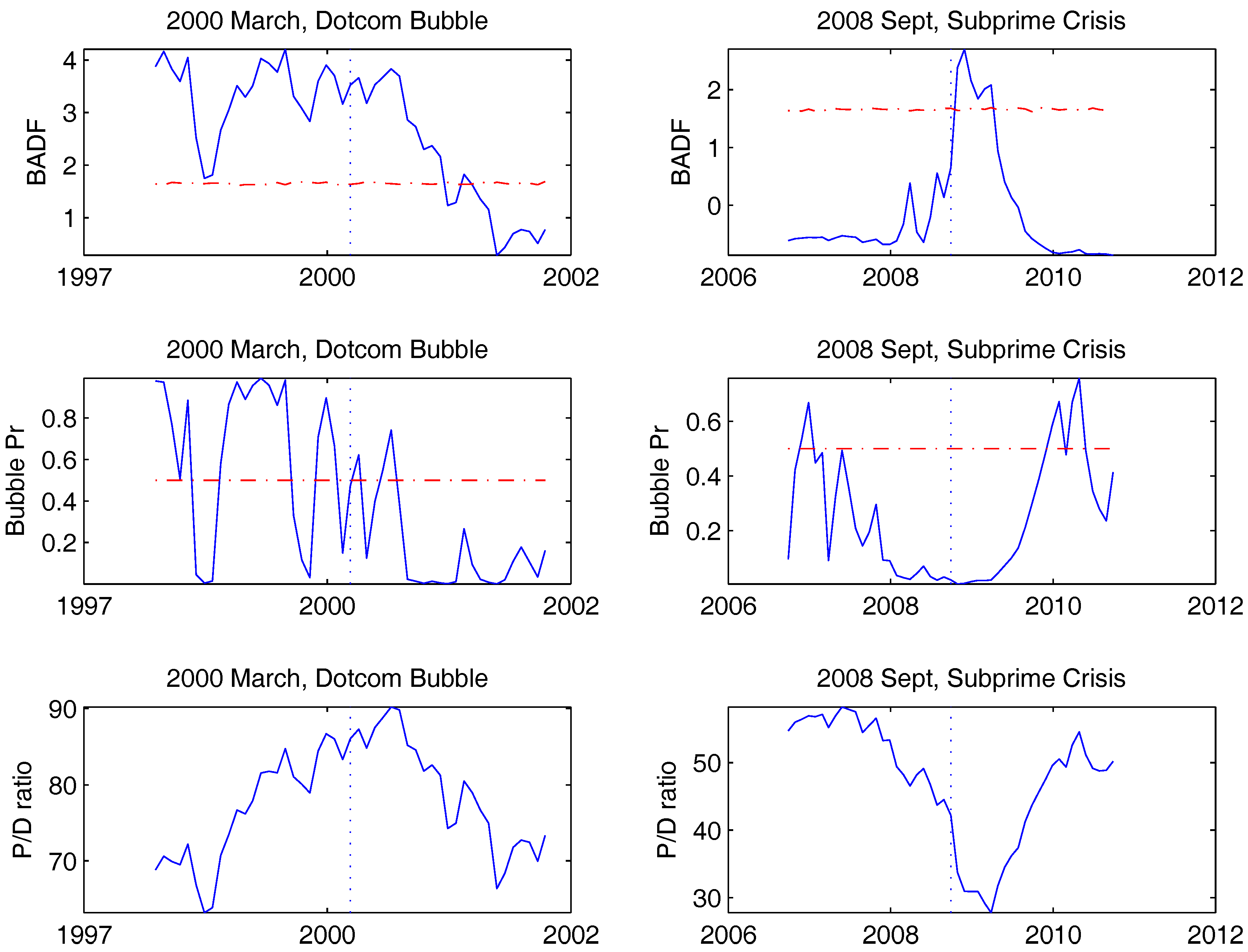
To better understand the behavior of the various bubble indicators, we take a microscopic view around well-known historical events. Here we focus on five events: The banking crisis in October 1907, the great market crash in September 1929, the Black Monday crash in October 1987, the DotCom mania peaking in March 2000 and the sub-prime crisis exploding in September 2008. Figure 6 and Figure 7 report both the PSY’s BSADF statistic (row 1), the filtered bubble probabilities from our regime-switching model (row 2) in the two years preceding and following these events. For reference row 3 depicts the original data series (price-dividend ratios) in the same periods. There are a few interesting patterns emerging from these graphs. First, both methods seem to indicate the presence of bubbles before the 1929 and 1987 crashes and during the DotCom bubble before 2000. A slight difference is that the regime-switching model seems to give more indication to the consecutive arrival of several shorter explosive periods, especially during the DotCom Mania. Second, the PSY method seems to have a difficulty in differentiating bubbles from collapses, a feature also noted in PSY (2015a). For instance, the BSADF statistic takes large positive values during the market collapse before October 1907 or in the months right after the Lehman bankruptcy in 2008. In contrast in the regime switching model the bubble regime probabilities stay low during these times. Third, the two methods interpret very differently when the market rallies after collapsing. For example, in months after October 1907 crash, after the 2000 crash, and the 2008 crash, the BSADF statistic actually decreases while the regime switching model sees explosive bubble periods.
5. Conclusions
In this paper, we propose a new regime switching model with two regimes, a normal regime and a bubble regime. To estimate the model we use a sequential Bayesian simulation method that allows for real time detection of bubble origination and conclusion. A particular feature of our framework is that it sequentially tracks the joint posterior distribution of the fixed parameters and of the hidden states. Hence, it properly allows for real time parameter uncertainty. The Monte Carlo evidence suggests that our method is reliable and robust to the presence of outliers and compares favorably to existing online methods in detection power. We carry out empirical study using real monthly S&P 500 price-dividend data. While some similar results have been obtained by PSY (2015a) in a classical setup and by our method, we find some differences in the two sets of empirical results. In particular, our method detects more bubble periods and can better discriminate between bubbles and collapses.
Acknowledgments
This article is dedicated to Peter C.B. Phillips, a giant in econometrics. We wish to thank the co-editors and two referees for helpful comments. Yu acknowledges support from the Singapore Ministry of Education for Academic Research Fund under grant number MOE2011-T2-2-096.
Author Contributions
Both authors contribute in setting up the model and the structure of the paper. Jun Yu is responsible for Section 1 and Section 2.1 and Andras Fulop for Section 2.2, Section 2.3, Section 2.4 and Section 2.5, Section 3 and Section 4.
Conflicts of Interest
The authors declare no conflict of interest.
References
- Ahamed, Liaquat. 2009. Lords of Finance: The Bankers Who Broke the World. New York: Penguin Press. [Google Scholar]
- Andrieu, Christophe, Arnaud Doucet, and Roman Holenstein. 2010. Particle Markov Chain Monte Carlo. Journal of Royal Statistical Society B 72: 1–33. [Google Scholar] [CrossRef]
- Busetti, Fabio, and A. M. Robert Taylor. 2004. Tests of stationarity against a change in persistence. Journal of Econometrics 123: 33–66. [Google Scholar] [CrossRef]
- Caballero, Ricardo J., Emmanuel Farhi, and Pierre-Olivier Gourinchas. 2008. Financial Crash, Commodity Prices and Global Imbalances. Brookings Papers on Economic Activity 2: 1–55. [Google Scholar]
- Campbell, John Y., and Robert J. Shiller. 1988. The dividend-price ratio and expectations of future dividends and discount factors. Review of Financial Studies 1: 195–227. [Google Scholar] [CrossRef]
- Chopin, Nicolas, Pierre E. Jacob, and Omiros Papaspiliopoulos. 2013. SMC2: An efficient algorithm for sequential analysis of state space models. Journal of the Royal Statistical Society B 75: 397–426. [Google Scholar] [CrossRef]
- Cochrane, John H. 2011. Presidential Address: Discount Rates. Journal of Finance 66: 1047–108. [Google Scholar] [CrossRef]
- Diba, Behzad T., and Herschel I. Grossman. 1988. Explosive rational bubbles in stock prices? The American Economic Review 78: 520–30. [Google Scholar]
- Evans, George W. Evans. 1991. Pitfalls in testing for explosive bubbles in asset prices. The American Economic Review 81: 922–30. [Google Scholar]
- Fearnhead, Paul. 1998. Sequential Monte Carlo methods in Filter Theory. Ph.D. thesis, University of Oxford, Oxford, UK. [Google Scholar]
- Fei, Y. 2017. Limit Theory for Mildly Integrated Process with Intercept. Working Paper, Singapore Management University, Singapore. [Google Scholar]
- Fulop, Andras, and Junye Li. 2013. Efficient learning via simulation: A marginalized resample-move approach. Journal of Econometrics 176: 146–61. [Google Scholar] [CrossRef]
- Godfeld, Stephen, and Richard Quandt. 1973. The Estimation of Structural Shifts by Switching Regressions. Annals of Economic and Social Measurement 2: 473–83. [Google Scholar]
- Funke, Michael, Stephen Hall, and Martin Sola. 1994. Rational bubbles during Poland’s hyperinflation: Implications and empirical evidence. European Economic Review 38: 1257–76. [Google Scholar] [CrossRef]
- Hall, Stephen G., Zacharias Psaradakis, and Martin Sola. 1999. Detecting Periodically Collapsing Bubbles: A Markov-Switching Unit Root Test. Journal of Applied Econometrics 14: 143–54. [Google Scholar] [CrossRef]
- Hamilton, James D. 1989. A new approach to the economic analysis of nonstationary time series and the business cycle. Econometrica 57: 357–84. [Google Scholar] [CrossRef]
- Homm, Ulrich, and Jörg Breitung. 2012. Testing for Speculative Bubbles in Stock Markets: A Comparison of Alternative Methods. Journal of Financial Econometrics 10: 198–231. [Google Scholar] [CrossRef]
- Jiang, Liang, Xiao hu Wang, and Jun Yu. 2017. In-Fill Asymptotic Theory for Structural Break Point in Autoregression: A Unified Theory. Working paper, Singapore Management University, Singapore. [Google Scholar]
- Kim, Jae-Young. 2000. Detection of change in persistence of a linear time series. Journal of Econometrics 95: 97–116. [Google Scholar] [CrossRef]
- Kohn, Donald L. 2008. Monetary Policy and Asset Prices Revisited. Paper presented at the Cato Institute’s 26th Annual Monetary Policy Conference, Washington, DC, USA, November 19. [Google Scholar]
- Lee, Ji Hyung, and Peter C. B. Phillips. 2016. Asset pricing withfinancial bubble risk. Journal of Empirical Finance 38: 590–622. [Google Scholar] [CrossRef]
- Phillips, Peter C. B., and Jun Yu. 2011. Dating the Timeline of Financial Bubbles During the Subprime Crisis. Quantitative Economics 2: 455–91. [Google Scholar] [CrossRef]
- Phillips, Peter C. B., Shu ping Shi, and Jun Yu. 2014. Specification Sensitivity in Right-Tailed Unit Root Testing for Explosive Behavior. Oxford Bulletin of Economics and Statistics 76: 315–33. [Google Scholar] [CrossRef]
- Phillips, Peter C. B., Shu ping Shi, and Jun Yu. 2015a. Testing for Multiple Bubbles: Historical Episodes of Exuberance and Collapse in the S&P500. International Economic Review 56: 1043–78. [Google Scholar]
- Phillips, Peter C. B., Shu ping Shi, and Jun Yu. 2015b. Testing for Multiple Bubbles: Limit Theory of Real Time Detector. International Economic Review 56: 1079–134. [Google Scholar] [CrossRef]
- Phillips, Peter C. B., Yang Ru Wu, and Jun Yu. 2011. Explosive behavior in the 1990s Nasdaq: When did exuberance escalate asset values? International Economic Review 52: 201–26. [Google Scholar] [CrossRef]
- Shi, Shu Ping. 2013. Specification Sensitivities in the Markov-Switching Unit Root Test for Bubbles. Empirical Economics 45: 697–713. [Google Scholar] [CrossRef]
- Shi, Shu Ping, and Yong Song. 2015. Identifying Speculative Bubbles with an Infinite Hidden Markov Model. Journal of Financial Econometrics 14: 159–84. [Google Scholar] [CrossRef] [Green Version]
- Wang, Xiao hu, and Jun Yu. 2015. Limit Theory for an Explosive Autoregressive Process. Economic Letters 126: 176–80. [Google Scholar] [CrossRef]
- Yiu, Matthew S., Jun Yu, and Lu Jin. 2013. Detecting Bubbles in Hong Kong Residential Property Market. Journal of Asian Economics 28: 115–24. [Google Scholar] [CrossRef]
| 1. | |
| 2. | A very recent contribution in deriving the asymptotic distribution for the change point estimator was made in Jiang et al. (2017). |
| 3. | In more recent attempts, Phillips et al. (2014), Wang and Yu (2015), Fei (2017) showed the impact of the intercept term on the asymptotics in various model setups. |
| 4. |
Figure 1.
Monte Carlo Results on Bubble Detection Rates of Online Learning vs PSY (2015a). This table reports how well the online Bayesian filter and the PSY (2015a) method perform in detecting bubble regimes as a function of the duration of the bubble. We execute a Monte Carlo exercise using three data generating processes. First, we run simulations using the true regime switching model as the data generating process. Second, to investigate the effect of outliers, we simulate data from a misspecified version with student-t innovations with 4 degrees of freedom. Third, we simulate from a DGP incorporating the leverage effect. For each DGP, we simulate 100 data sets with 1,698 observations. The uppermost panel shows the average frequency of periods flagged as bubble among the time periods that are in fact in the bubble regimes since n periods when the DGP from our regime switching model is used to generate the data. The solid lines depict the detection rates from our online Bayesian filter. The flat line corresponds to a stamping rule of , the one with circles to while the one with crosses to . The dotted line presents the detection rates from the PSY (2015a) method. The middle panel reports analogous results when a misspecified DGP with student-t innovations with 4 degrees of freedom is used, while the lower panel shows the results when a misspecified DGP with the leverage effect is used.

Figure 2.
S&P 500 Price-Dividend Ratio. This figure shows the monthly real S&P 500 price-dividend data between January 1871 to June 2012.
Figure 2.
S&P 500 Price-Dividend Ratio. This figure shows the monthly real S&P 500 price-dividend data between January 1871 to June 2012.

Figure 3.
Histogram of parameter priors and posteriors. This figure reports the histogram of the priors (in blue) and the full-sample posteriors (in red). The sample is monthly S&P 500 price-dividend data between January 1871 to June 2012.
Figure 3.
Histogram of parameter priors and posteriors. This figure reports the histogram of the priors (in blue) and the full-sample posteriors (in red). The sample is monthly S&P 500 price-dividend data between January 1871 to June 2012.

Figure 4.
Bubble Regimes from Bayesian Learning. This figure reports the real-time bubble regimes indicated by our regime switching model together with the filtered bubble regime probability. A given month is classified as belonging to the bubble regime if this latter is the regime with the highest filtered probability. The plot corresponds to the bubble stamping parameter . Bubble regimes are the shaded grey areas. The sample is monthly S&P 500 price-dividend data between January 1871 to June 2012.

Figure 5.
Bubble Regimes from recursive regressions as in PSY (2015a). This figure reports the real-time bubble regimes indicated the backward sup ADF (BSADF) statistics from PSY (2015a). A given month is deemed to belong to a bubble regime if the value of the BSADF statistic exceeds where is the critical value of the test statistic. Bubble regimes are the shaded grey areas while the solid line depicts the BSADF sequence. The sample is monthly S&P 500 price-dividend data between January 1871 to June 2012.

Figure 6.
Behavior of bubble detectors around historical events: I. This figure reports the behavior of both the PSY and our regime-switching bubble indicators around some well-known historical events. The event itself is always shown by a vertical dashed line. Each time we report two years before and two years after the event. The first row reports the PSY BSADF statistic together with in dashed red. The second row reports the filtered bubble probabilities from our regime-switching model. The last row shows the data, the real S&P 500 price-dividend ratio.

Figure 7.
Behavior of bubble detectors around historical events: II. This figure reports the behavior of both the PSY and our regime-switching bubble indicators around some well-known historical events. The event itself is always shown by a vertical dashed line. Each time we report two years before and two years after the event. The first row reports the PSY BSADF statistic together with the critical values in dashed red. The second row reports the filtered bubble probabilities from our regime-switching model. The last row shows the data, the real S&P 500 price-dividend ratio.


Table 1.
Monte Carlo Results on Posterior Parameter Estimates.
| Parameters | True | Post. Mean | Post. Credible Interval | Prior Credible Interval |
|---|---|---|---|---|
| 150 | 189.4 | 126.9 | 153.7 | |
| 1.8 | 1.91 | 1.68 | 1.87 | |
| 30 | 35.95 | 21.15 | 31.01 | |
| 0.98 | 0.97 | 0.01 | 0.89 | |
| 0.94 | 0.93 | 0.049 | 0.90 | |
| 0.65 | 0.65 | 0.04 | 2.7 | |
| 2.8 | 2.77 | 0.37 | 1.88 | |
| 0.3 | 0.214 | 0.428 | 0.477 | |
| 0.99 | 0.989 | 0.006 | 0.025 | |
| 1.015 | 1.014 | 0.005 | 0.0180 |
This table reports various statistics from the Monte Carlo exercise using the true regime switching model as the data generating process, where we simulate 100 data sets with 1698 observations. The first column reports the true parameter values, the second column the average posterior means across the 100 data sets, the third column the average length of the posterior central credible interval across the 100 runs and the fourth column the prior credible interval.
Table 2.
Monte Carlo Bubble Detection Statistics.
| Methods | Number of Bubble Spells | Total Bubble Length/T | Avg Bubble Duration in Months |
|---|---|---|---|
| Realized numbers | |||
| 9.07 | 0.164 | 30.24 | |
| Panel A: Correctly Specified DGP | |||
| PSY | 13.2 | 0.095 | 11.0 |
| RS, | 17.4 | 0.095 | 8.9 |
| RS, | 8.6 | 0.091 | 17.3 |
| RS, | 6.9 | 0.087 | 20.6 |
| Panel B: Misspecified DGP with Fat Tails | |||
| PSY | 13.8 | 0.096 | 11.0 |
| RS, | 19.9 | 0.106 | 8.7 |
| RS, | 10.0 | 0.102 | 17.0 |
| RS, | 8.0 | 0.099 | 21.0 |
| Panel C: Misspecified DGP with Leverage | |||
| PSY | 13 | 0.090 | 11.3 |
| RS, | 16.1 | 0.090 | 9.42 |
| RS, | 7.91 | 0.086 | 18.37 |
| RS, | 6.49 | 0.082 | 21.77 |
This table reports summary statistics on the different bubble-stamping procedures in a Monte Carlo exercise using three data generating processes. First, we run simulations using the true regime switching model as the data generating process. Second, to investigate the effect of outliers, we simulate data from a misspecified version with student-t innovations with 4 degrees of freedom. Third, we simulate a DGP with a leverage effect. For each DGP, we simulate 100 data sets with 1698 observations. In all panels, the first row reports the results from the PSY (2015a) procedure while rows 2-4 report the results from our regime switching model at different values of the bubble stamping parameter . In all cases the figures are average numbers across the 100 simulations.
Table 3.
Full Sample Posterior Parameter Estimates for S&P 500.
| Parameters | Posterior Mean | Posterior 5th Prctile | Posterior 95 Prctile |
|---|---|---|---|
| 147 | 123.5 | 183.1 | |
| 1.795 | 1.152 | 2.589 | |
| 30.74 | 25.25 | 38.31 | |
| 0.9842 | 0.9754 | 0.9907 | |
| 0.9412 | 0.9128 | 0.963 | |
| 0.6694 | 0.6367 | 0.7017 | |
| 2.895 | 2.708 | 3.1 | |
| 0.3117 | 0.09392 | 0.6485 | |
| 0.99 | 0.9784 | 0.9982 | |
| 1.015 | 1.01 | 1.018 |
This table reports the full sample posterior estimates of the full model on monthly S&P 500 price-dividend data between January 1871 to June 2012.
Table 4.
Bubble Detection Statistics for S&P 500.
| Methods | Number of Bubble Spells | Total Bubble Length/T | Avg Bubble Duration in Months |
|---|---|---|---|
| PSY | 22 | 0.056 | 4.27 |
| RS, | 58 | 0.16 | 4.5 |
| RS, | 24 | 0.14 | 9.7 |
| RS, | 20 | 0.125 | 10.4 |
This table reports summary statistics on the different bubble-stamping procedures for monthly S&P 500 price-dividend data between January 1871 to June 2012. The first row reports the results from the PSY (2015a) procedure while rows 2–4 report the results from our regime switching model at different values of the bubble stamping parameter .
© 2017 by the authors. Licensee MDPI, Basel, Switzerland. This article is an open access article distributed under the terms and conditions of the Creative Commons Attribution (CC BY) license (http://creativecommons.org/licenses/by/4.0/).
Share and Cite
MDPI and ACS Style
Fulop, A.; Yu, J. Bayesian Analysis of Bubbles in Asset Prices. Econometrics 2017, 5, 47. https://0-doi-org.brum.beds.ac.uk/10.3390/econometrics5040047
AMA Style
Fulop A, Yu J. Bayesian Analysis of Bubbles in Asset Prices. Econometrics. 2017; 5(4):47. https://0-doi-org.brum.beds.ac.uk/10.3390/econometrics5040047
Chicago/Turabian StyleFulop, Andras, and Jun Yu. 2017. "Bayesian Analysis of Bubbles in Asset Prices" Econometrics 5, no. 4: 47. https://0-doi-org.brum.beds.ac.uk/10.3390/econometrics5040047
Note that from the first issue of 2016, this journal uses article numbers instead of page numbers. See further details here.