
Reducing Approximation Error in the Fourier Flexible Functional Form

Department of Agricultural and Resource Economics, College of Agriculture and Bioresources, Agriculture Building, University of Saskatchewan, Rm 3D24, Saskatoon, SK S7N 5A8, Canada
Econometrics 2017, 5(4), 53; https://0-doi-org.brum.beds.ac.uk/10.3390/econometrics5040053
Submission received: 29 August 2017
/
Revised: 16 November 2017
/
Accepted: 22 November 2017
/
Published: 4 December 2017
Abstract
:The Fourier Flexible form provides a global approximation to an unknown data generating process. In terms of limiting function specification error, this form is preferable to functional forms based on second-order Taylor series expansions. The Fourier Flexible form is a truncated Fourier series expansion appended to a second-order expansion in logarithms. By replacing the logarithmic expansion with a Box-Cox transformation, we show that the Fourier Flexible form can reduce approximation error by 25% on average in the tails of the data distribution. The new functional form allows for nested testing of a larger set of commonly implemented functional forms.
JEL Classification:
C51; D24; Q121. Introduction
Functional form selection can be difficult in applied work, especially in cases where economic theory is not a useful guide. The Fourier flexible form of Gallant (1981, 1982) has been a preferred solution in many cases, as it allows for global approximations to the underlying theoretical counterpart. However, there is high potential for approximation error resulting from boundary and edge effects when approximating non-periodic data, as is often the case in economic applications. The purpose of this article is to develop a new functional form based on the existing Fourier flexible form that will address this issue while maintaining the desirable characteristics of the original.
From the early 1970’s, Diewert-flexible forms such as the generalized Leontief, quadratic (normalized, square-rooted and symmetric) and translog have dominated applied parametric analysis. These functional forms have many desirable properties, placing no restrictions on derived measures that are functions of their first and second derivatives (Creel 1997).1 However, they are based on second-order Taylor series approximations, which are local in nature. Unless the true function subject to approximation happens to be in the same family as the approximating function, least squares will not consistently estimate the true value of the function in a global sense (White 1980). This limitation was addressed by Gallant’s (1981, 1982) Fourier flexible form. Based on the composition of a truncated Fourier series expansion of orthogonal polynomials and a second-order Taylor-series expansion in logarithms, the Fourier flexible form can provide an arbitrarily close, global approximation to an unknown function (Gallant 1982).
The form has seen applications in many areas of economics, including agriculture and production (Chalfant 1984; Ivaldi et al. 1996; Skolrud and Shumway 2013; Fleissig 2015), banking and stock price variation (Mitchell and Onvural 1996; Berger and Mester 1997; Huang and Wang 2004a; Huang and Wang 2004b; Park 2010), the measurement of welfare (Creel 1997) and the estimation of stochastic volatility demand systems (Serletis and Isakin 2017). It has also been used to estimate structural breaks in time series data when the number of breaks and the functional form of the break is unknown to the researcher (Becker et al. 2006). Enders and Lee (2012a, 2012b) use the Fourier flexible form to construct unit root tests that do not require a priori knowledge of the precise form of the break. These tests have been employed in a variety of applications, including tests of stationarity in house prices (Chang et al. 2015) and real exchange rates (Zhou and Kutan 2014).
Despite its reduction in specification error, the Fourier flexible form is still subject to approximation error (Mitchell and Onvural 1996). The approximation error results from two sources: using trigonometric regression terms to estimate a non-periodic function and Fourier approximation with a finite order of approximation (i.e., Gibbs phenomenon). Due to finite sample sizes, virtually all applications in economics require a truncated Fourier series, i.e., a finite order of approximation and most applications employ non-periodic relationships, so these two sources of approximation error are frequently present.
To solve this problem, we replace the second-order logarithmic expansion with a second-order expansion in the Box-Cox polynomial. As evidenced by Eubank and Speckman (1990), including a low-order polynomial in a trigonometric regression (such as a Fourier series approximation) can dramatically reduce approximation error. The exact low-order polynomial that minimizes the approximation error is dependent on the data generating process and simulation results from Eubank and Speckman (1990) demonstrate that the precise order can vary widely. By using the Box-Cox function in place of the logarithmic, the ideal low-order polynomial that reduces approximation error will be revealed by the true data generating process.
In introducing the Box-Cox modification, we also allow for a much wider range of nested testing possibilities. With the exception of the likelihood dominance test of Skolrud and Shumway (2013), the Fourier flexible form has only been tested against its nested alternatives—the translog and Cobb-Douglas. With the new functional form, robust, nested testing is possible for a wide variety of popular functional forms.
Simulation evidence demonstrates that the new functional form, referred to as the Box-Cox Fourier flexible form, significantly reduces boundary approximation bias relative to the original Fourier flexible form. Likelihood ratio tests demonstrate the superiority relative to the original and to the translog in terms of overall fit. The ability of the new functional form to reduce the bias is tested for multiple data generating processes, orders of Fourier series approximations and error distributions.
2. Materials and Methods
The Fourier flexible form is preferable to its Diewert-flexible competitors due to its ability to represent an unknown function as closely as desired in terms of the Sobolev norm, which is a global measure of distance between two functions as well as their derivatives.2 Parameter estimates based on Diewert-flexible forms are subject to the maintained hypothesis that the true unknown function is derived from the same family of functions used in the approximation (White 1980; Gallant 1981).3 The fact that the Fourier flexible form is not subject to this maintained hypothesis makes it an extremely desirable alternative, as we can never know if the maintained hypothesis is in fact valid. These facts are well-known and clearly documented in the literature for a variety of cases. The important statistical properties are proven in Gallant (1981, 1982), Elbadawi et al. (1983) and Eastwood and Gallant (1991).
In this article, we take the desirable statistical properties of the original Fourier flexible form as given and provide only a brief description as it pertains to our suggested modification. Interested readers should consult the previously mentioned articles for more details on the statistical properties of the Fourier flexible form, along with less-technical summaries available in Creel (1997), Mitchell and Onvural (1996) and Ivaldi et al. (1996).
For ease of exposition, we present the Fourier flexible form as a cost function, similar to Gallant (1982). Let be the cost function resulting from a perfectly competitive firm’s cost minimization problem, where is a vector of n input prices and is a vector of m output quantities. The Fourier flexible form of the cost function is given by:
where is a dimensional vector of scaled input prices and output quantities, is a vector of parameters, is an integer-valued dimensional vector, is the number of vectors and is a stochastic disturbance term with mean 0 and variance .4 Note that the data vector must be scaled to fit in the interval ] in order to be expanded in the Fourier series approximation. In Gallant’s (1982) formulation, the vector is composed of logarithmic scaled input prices and output quantities.
The Fourier flexible form is comprised of a second-order polynomial appended to a Fourier series. While the Fourier series component is sufficient for close approximation in the Sobolev norm, the addition of the polynomial serves to (1) limit the number of required Fourier series terms, (2) allow for nested testing of the translog and Cobb-Douglas functional forms and (3) decrease approximation error at the boundaries of the domain (Gallant 1981, 1982; Gallant and Souza 1991). In the next section, we argue that a generalization of this polynomial allows for further reductions in approximation error and allows for a wider range of nested tests of functional form.
Consider the following modification of the Fourier flexible form presented in Equation (1):
where is an vector of scaled input prices and output quantities and and are Box-Cox transformations, defined as:
and all other variables are as previously defined. In previous uses of the Fourier flexible form, would be expressed in logarithms; this approach relaxes this restriction. Note however that as , , and become and , respectively and the Box-Cox Fourier flexible form becomes the Fourier flexible form.
There are two important benefits resulting from the extra flexibility afforded by the Box-Cox polynomial expansion. The most important benefit is the reduction in approximation error. In their paper analyzing the improvement provided by appending low-order polynomials to trigonometric expansions (truncated Fourier series), Eubank and Speckman (1990) demonstrate that the boundary approximation can be dramatically improved but the improvement is dependent on the order of the polynomial. By choosing the Box-Cox parameters and parametrically, our new form can adjust to reduce the boundary approximation error. The second benefit concerns the nested testing of popular functional form alternatives. By choosing a second-order polynomial expansion in logarithms, the original construction (Gallant 1982) nests the popular translog functional form (Christensen et al. 1975), which in turn nests the Cobb-Douglas functional form. This choice allowed researchers to make a robust, nested comparison to two of the most popular functional form alternatives. Many studies using the Fourier flexible form in an empirical setting make the comparison to the translog and an extensive search did not find any study that failed to reject the translog based on statistical test. Our modification continues to allow this important nested test, as well as the nested testing of several more functional forms through appropriate modifications of and . They include the TLF, translog, Generalized Box-Cox, linear, normalized quadratic, generalized Leontief, modified resistance, non-homothetic CES (Applebaum 1979), logarithmic and Cobb-Douglas.5 The parametric restrictions required to produce these functional forms are listed in Table 1.
To obtain these benefits, we have introduced two nonlinear parameters, which will require a more complicated estimation technique compared to the Fourier flexible form. Fortunately, the Box-Cox polynomial has seen frequent use in economics, so appropriate estimation procedures are well developed. Our estimation technique relies on existing procedures with only minor modifications to allow for the estimation of Fourier series parameters. In the following exposition, we will refer to the Fourier flexible form of Gallant (1982) as the TLF, to reflect its nesting of the translog and we will refer to the Box-Cox Fourier flexible form as the BCF, to reflect its nesting of the Box-Cox polynomial.
One of the advantages of the TLF is that despite its complexity, it is still linear in parameters, so ordinary least squares can be used with no inherent complications. The BCF has two nonlinear parameters, and . Using maximum likelihood estimation, these parameters (and the remaining parameters) in the model can be recovered with relative ease.
First, we collect the right-hand side variables into the matrix , such that includes the second-order expansion in and the 2A trigonometric terms. The number of trigonometric terms to include is governed by several factors, including the sample size, order of approximation of the Fourier series component and the number of input prices and output quantities. We discuss these factors and selection of multi-indices in the Appendix A.
We can write the BCF compactly as . If we expect the error to be normally distributed, we can write the likelihood function as:
The log-likelihood is given by:
Instead of choosing all parameters in the vector , , and simultaneously, we can “concentrate out” most of them and greatly simplify the optimization process. Concentrating out a parameter from an objective function involves replacing the parameter with its optimal solution from solving the system of first-order conditions. This process embeds the optimal choice of the parameter in the objective function itself. The first-order conditions from choosing and to maximize (5) can be solved to yield the usual estimators, and , where is the vector of residuals, .
Before both and are concentrated out, we need to concentrate out just so that the information matrix can be derived to yield the standard errors for the estimated parameters. Denote the log-likelihood with concentrated out as :
The first-order conditions from the maximization of (6) are as follows:
where subscripts indicate partial derivatives with respect to the subscripted argument and is a vector of ones. The Hessian matrix, derived from the system of first-order conditions, is given by:
The inverse of the negative of the Hessian matrix in (8), evaluated at the parameter values that maximize (6), is the estimated covariance matrix of the parameter estimates. As noted in Spitzer (1982), use of as the covariance matrix for instead of would lead to an underestimation of the standard errors, due to the neglected variance from the and
The estimation problem can be further simplified by concentrating out from the log-likelihood function. Denote this concentrated likelihood function by :
Now the problem has been reduced to a choice of just two parameters, not the entire set of parameters. Denote the values of and that maximize (9) as and , respectively. Then, the optimal is given by . This method is equivalent to solving a series of least squares problems for varying values of and If the assumption of a normal distribution is deemed too restrictive for a given application, alternative estimation strategies can be implemented, such as nonlinear least squares, or a grid search for the optimal values of and followed by ordinary least squares.
To assess the ability of the BCF to mitigate approximation error compared to the TLF, we turn to Monte Carlo simulations. We generate input price and output quantity data using fixed parameter values and total cost is derived from several data generating processes. We impose symmetry and linear homogeneity on the generated cost function through price normalization and proper multi-index selection (discussed in the Appendix A). Concavity is not imposed a priori to maintain second-order flexibility and to not confound simulation results. As robustness checks, we conduct simulations with errors from two different distributions.
To prevent the BCF from having an a priori advantage over the TLF in estimation, we choose data generating processes that are not nested in the generalized Box-Cox (and consequently not nested in the BCF). We use the generalized Cobb-Douglas function (Fuss et al. 1978):
the resistance function (Heady and Dillon 1961):
and the generalized quadratic function (Denny 1974):
We consider two distributions for the generation of the error term —standard normal and Laplace. Errors from the standard normal distribution are used as a baseline comparison and are consistent with the likelihood function developed in the previous section. The Laplace distribution is used as a comparison due to its high kurtosis (thick tails), which we expect will exacerbate boundary approximation issues. For this reason, we expect the fit of the TLF relative to the BCF to be even worse in the case of Laplace errors. To estimate parameters of the BCF when the errors are distributed Laplace, we use nonlinear least squares with estimates from the corresponding maximum likelihood estimation as starting values.
Additionally, we use second, third and fourth-order Fourier series approximations for comparison. As the order of approximation increases and the TLF and BCF both improve in overall fit, we hypothesize that the relative advantage of the BCF over the TLF will diminish. This is due to the reduction in approximation error resulting from Gibbs Phenomenon, a “wringing” effect that subsides as the order of approximation increases (Eubank and Speckman 1990; Jerri 1998). Due to the semi-nonparametric estimation, the sample size must change along with the order of approximation. To determine the appropriate sample size to use in the data generating process, we use the rule proposed by Eastwood and Gallant (1991), which suggests selecting a total number of parameters equal to the sample size raised to the two-thirds power. Combined with the rules governing multi-index selection discussed in the Appendix A, we can derive the appropriate sample size for each order. Using these rules, second, third and fourth-order Fourier approximations require sample sizes of 333, 1348 and 5405, respectively.
As one instance of economic relevance, we design a simulation to estimate returns to scale at each observation of the generated data. We compare estimates of economies of scale from the BCF and the TLF to the true economies of scale values and then conduct hypothesis tests to see the frequency with which each form correctly rejects increasing, constant, or decreasing returns to scale at several observations in the sample data. We use the multi-product economies of scale measure, , from Baumol et al. (1982), where with indicating the derivative of the cost function with respect to output j.
3. Results
We first compare the fit of the BCF to the simulated data using likelihood ratio tests, which we report in Table 2. Hypothesis tests are conducted against the null of the TLF and translog (TL) for each data generating process and for three increasing orders of Fourier series approximation. With a second-order approximation, the TL is rejected in favor of the BCF at the 1% level of significance for all data generating processes, while the TLF is rejected in favor of the BCF at the 5% level for one data generating process (resistance) and at the 1% level for the remaining two. As the order of approximation in the Fourier series increases, the TLF is still rejected in favor of the BCF, albeit at a lower level of significance for two of the three data generating processes. The TL is rejected in favor of the BCF at the 1% level of significance in eight of the nine scenarios and at the 5% level in the final scenario.
Table 3 shows the percentage reduction in the cost estimation bias from using the BCF and TLF estimates for each data generating process and for second, third and fourth-order Fourier series approximations when the errors are standard normal. Estimation bias is measured as the absolute value of the bias between the true cost function and the estimated function. Bias reductions are split into two columns for each data generating process/order of approximation combination: the average in percentage bias reduction over the bottom 10% of sorted observations and the average over the top 10% of sorted observations. When the data is generated from the generalized Cobb-Douglas function, the second-order BCF reduces the approximation bias by over 27% compared to the TLF over the bottom 10% of observations and reduces the bias by 24% over the top 10% of observations. When the resistance function is used as the data generating process, the gain from using the BCF is smaller, with a range of bias reduction between 15% and 17%. The results from using the generalized quadratic is just the opposite, with reductions in bias of greater than 35% from using the BCF. We suspect that this is due to the complexity of the data generating processes: compared to the generalized Cobb-Douglas, the resistance function is simpler (fewer parameters) and the generalized quadratic is more complex (more parameters, highly nonlinear).
When the order of approximation is increased in the BCF and TLF, the relative advantage of the BCF shrinks. For a third-order approximation, the average percentage bias reduction ranges from 7% to 25% and for a fourth-order approximation, the bias reduction ranges from 5% to 19%. The relationship in bias reduction across data generating processes remains consistent across the increasing approximation orders.
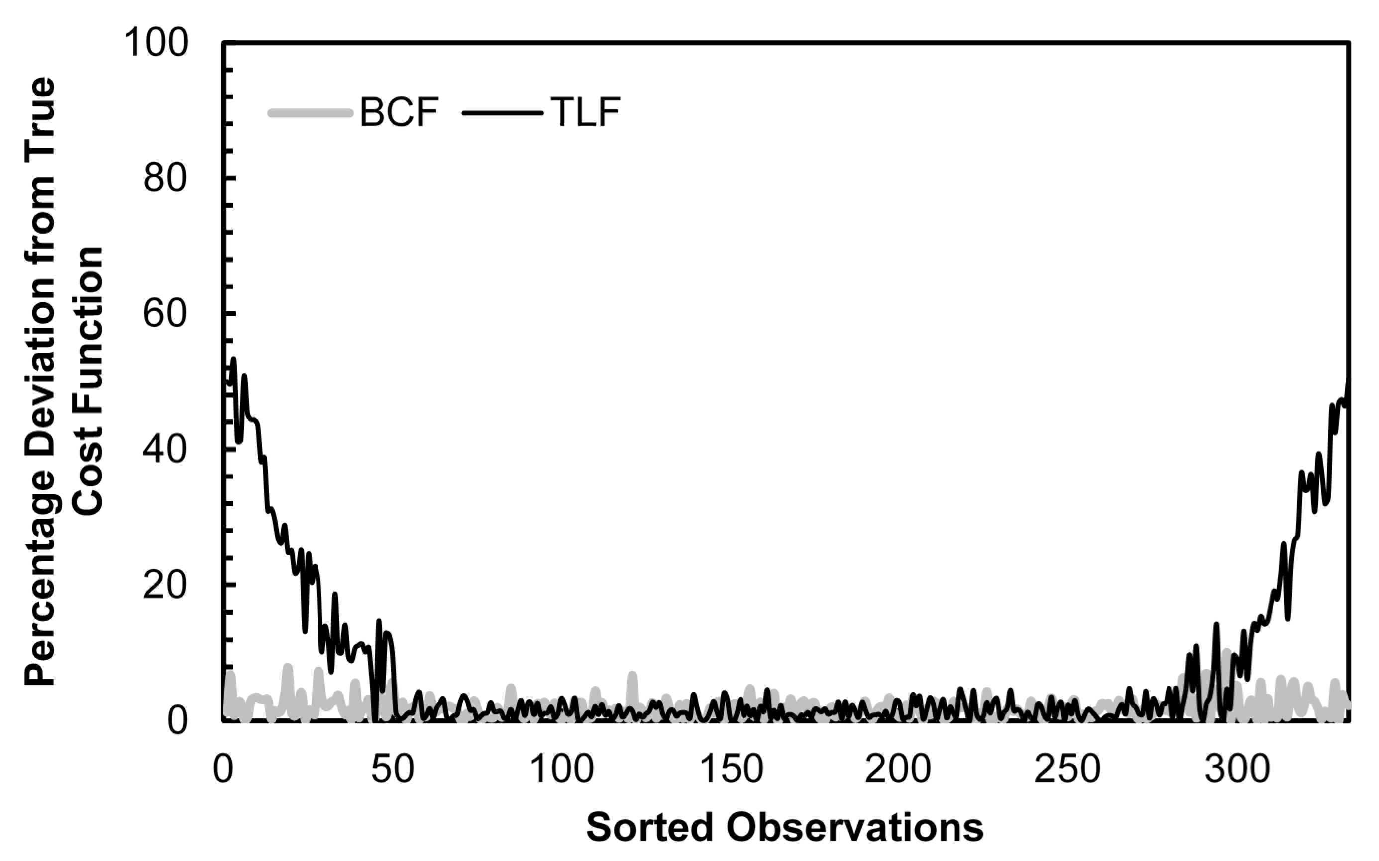
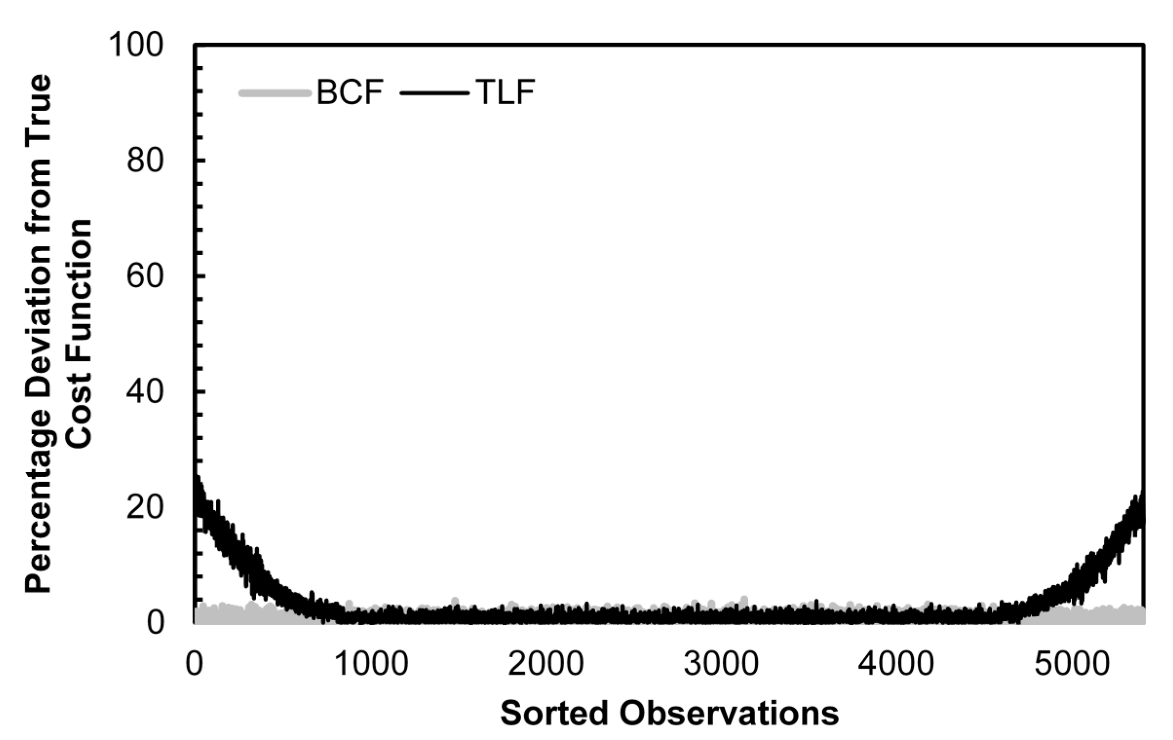
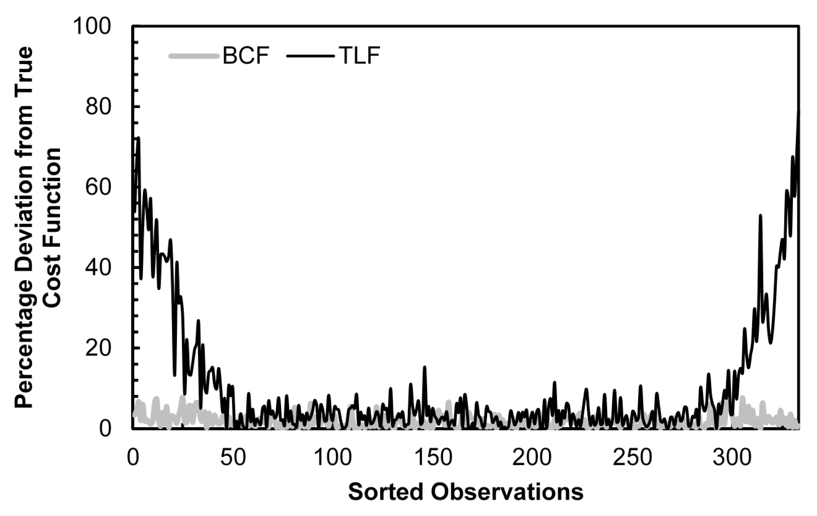
Figure 1 provides a graphical representation of the percentage deviation from the true cost function for the BCF and TLF estimates using the generalized Cobb-Douglas data generating process, a second-order Fourier series approximation and normally distributed random errors. The horizontal axis shows observations sorted in order of increasing total cost. From the figure, we can see that the percentage deviation of the BCF remains low throughout the entire domain, while the TLF shows very large deviations at the boundaries of the domain. For the smallest observation, the TLF has a bias of about 50% while the BCF bias is only about 8%, a 5/6 drop. For the largest observation, the effect is even greater, at least a 9/10 drop.
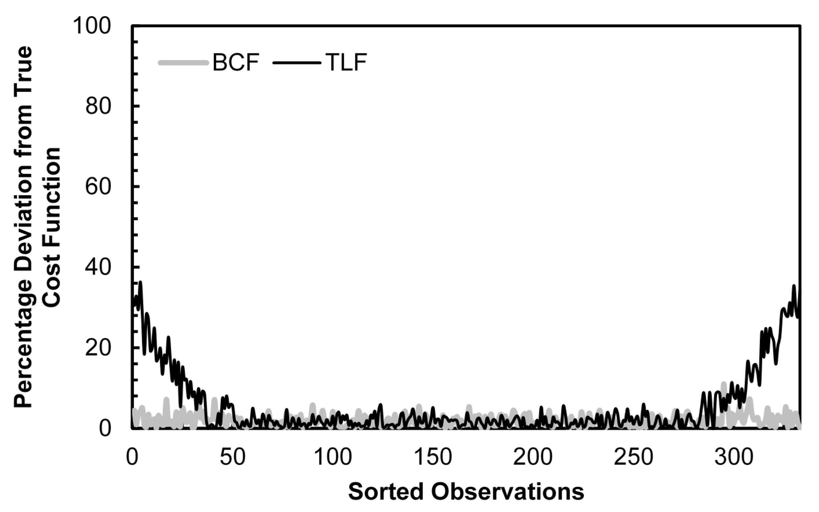
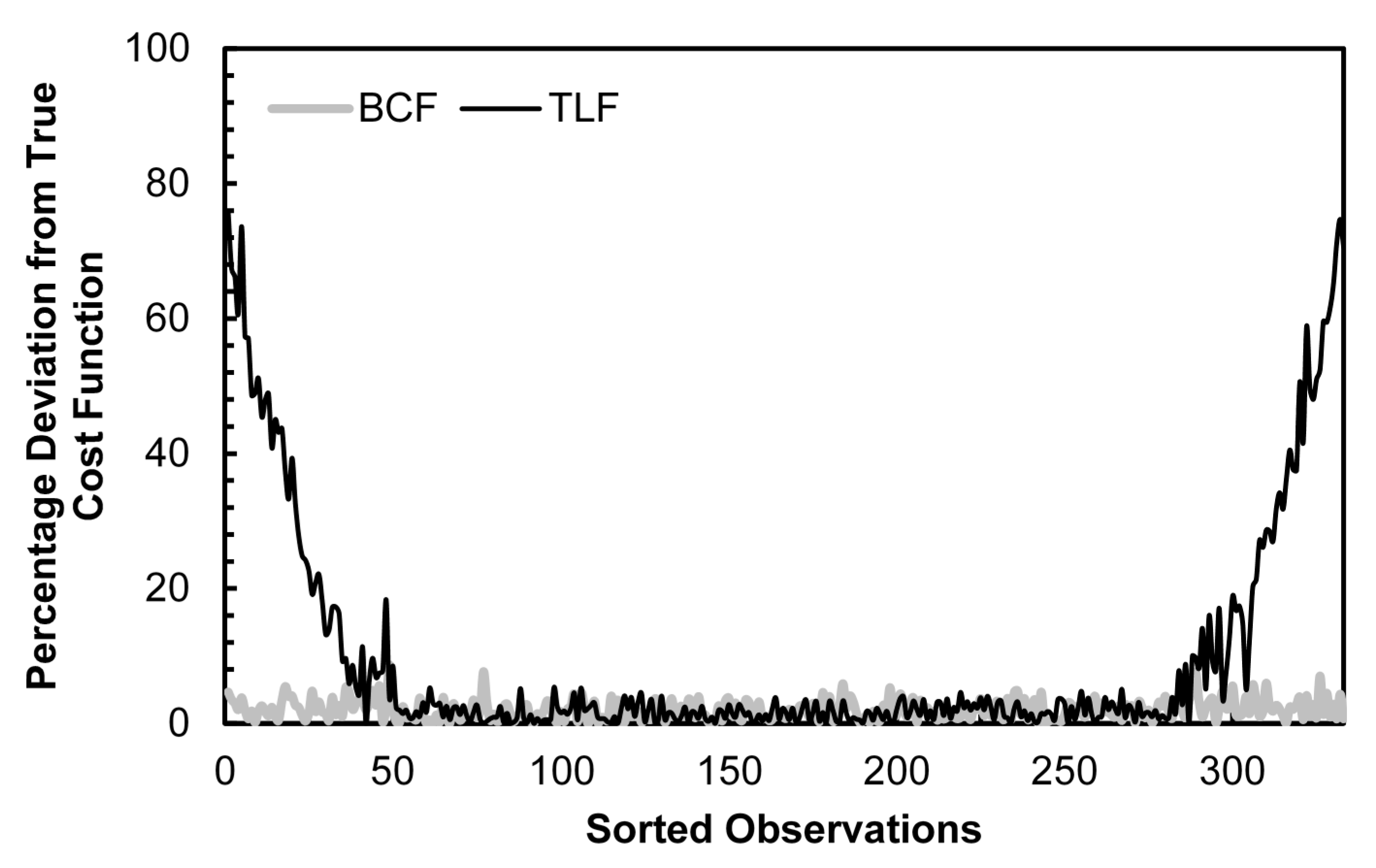
Figure 2 demonstrates the estimation bias for the resistance function data generating process and Figure 3 shows the bias for the generalized quadratic. Both figures provide visual confirmation of the results in Table 3: the BCF bias is a small fraction of the TLF bias for the smallest and largest observations and the TLF bias is higher when the generalized quadratic data generating process is used and lower when the resistance function is used.
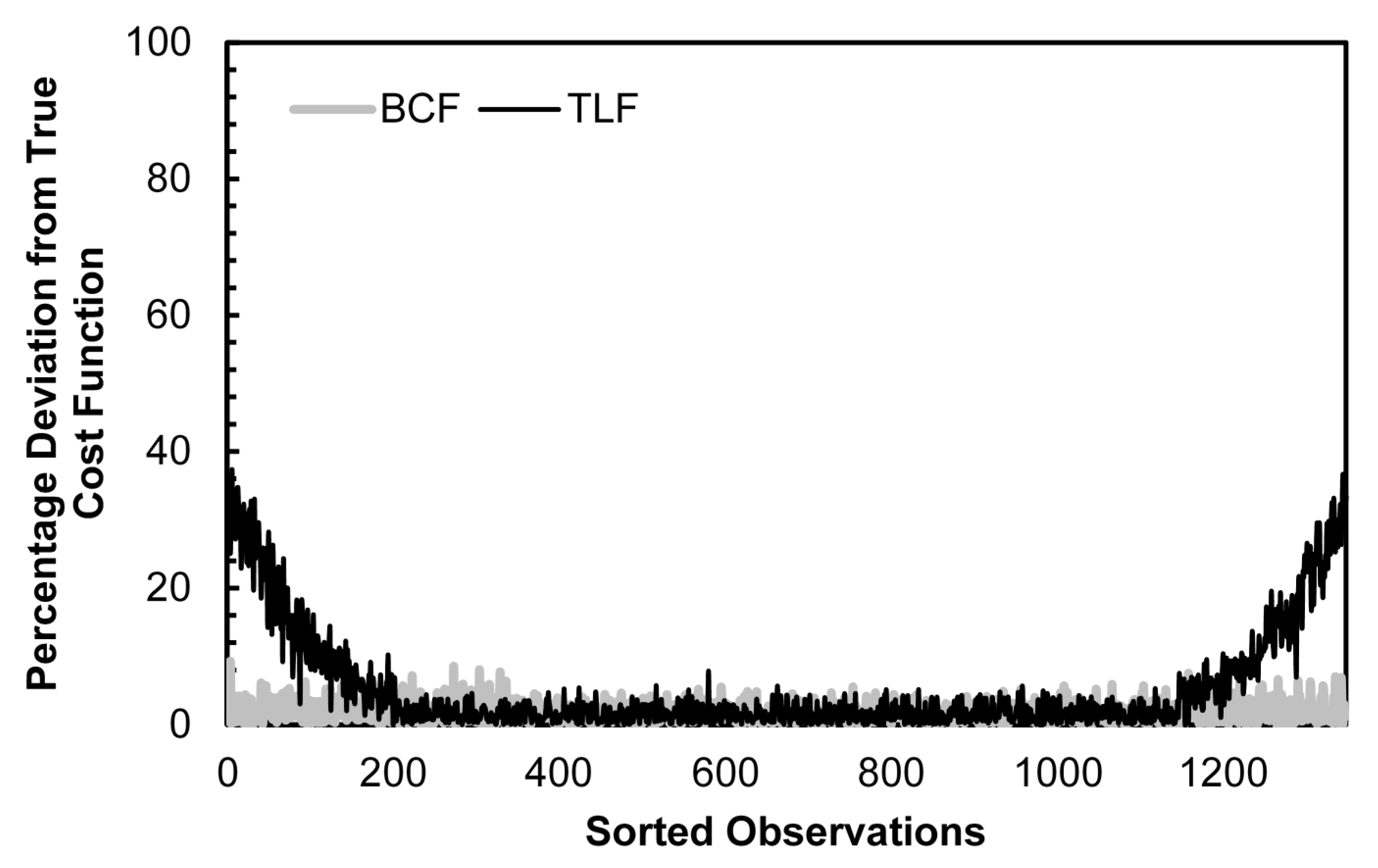
Figure 4 and Figure 5 demonstrate the difference in bias when the approximation order of the Fourier series increases to three and four, respectively. Note that in each figure, the sample size has increased to accommodate the semi-nonparametric estimation. Compared to Figure 1, Figure 4 shows a decrease in TLF bias at the domain boundaries. In Figure 5, the TLF bias is even smaller as the order of approximation increases to four.
In Table 4, we conduct the same simulations and analysis as reported in Table 3 for the case of Laplace distributed random errors (mean = 0, standard deviation = 1). We use the Laplace distribution due to its excess kurtosis, which is equal to six (kurtosis for the standard normal is three). With higher kurtosis, a greater proportion of the observations will be concentrated at the tails of the data and Table 4 demonstrates the extent to which this excess kurtosis exacerbates the boundary issue. For a second-order Fourier series approximation using the generalized Cobb-Douglas data generating process, the percentage reduction in bias increases to a range of 31% to 34%, up from a range of 24% to 27% under normally distributed errors. With the most complex data generating process considered, the generalized quadratic, the reduction in bias from using the BCF is nearly double that under normally distributed errors. We note that the relationships revealed by Table 3 continue in Table 4: bias reduction improves with more complex data generating processes and diminishes as the order of approximation increases. Figure 6 provides a graphical representation of the BCF and TLF bias for a generalized Cobb-Douglas data generating process and second-order Fourier approximation with errors distributed Laplace. The difference in approximation error compared to the normal distributed error case shown in Figure 1 is striking, with the TLF deviating from the true cost function by as much as 70% for the smallest and largest observations.
We note that in each simulation considered, the difference in bias present in both the BCF and TLF in the middle 80% of the data is small, with the BCF outperforming the TLF in the majority of cases by less than 1%. These results are documented in Table 5. In two cases, (case 1: 3rd order approximation, generalized quadratic data generating process, normally distributed errors; case 2: 4th order approximation, generalized Cobb-Douglas data generating process, Laplace distributed errors) the TLF slightly outperforms the BCF but by less than 0.1% in either case. This means that when statistics using the data means are the only ones of interest, using the BCF provides only a minimal advantage in reducing bias. However, when estimates involving the top and bottom deciles of the domain are important, our simulation results suggest that the BCF will provide a dramatic reduction of approximation bias over the TLF.
Finally, we report results from a scenario where the approximation bias of the TLF can lead to a misinterpretation with important economic implications. In Table 6, we present economies of scale estimates by data generating process estimated by the TLF and BCF. Estimates are split in two columns: the bottom 10% and top 10% columns give average economies of scale estimates for the smallest 10% and largest 10% of observations, respectively. Bootstrap standard errors are shown in parentheses below each estimate. The true average economies of scale estimate is shown at the bottom of each column. In this simulation, the data and parameters are generated such that the average economies of scale over the bottom 10% of observations is 1.10 (increasing returns to scale) and the average economies of scale over the top 10% of observations is 0.90 (decreasing returns to scale).
We conduct hypothesis tests to determine if estimates from the TLF and BCF properly reject constant returns to scale in favor of increasing returns over the bottom 10% of observations and if they properly reject constant returns to scale in favor of decreasing returns over the top 10% of observations. The TLF properly rejects constant returns in favor of increasing returns at the 10% level of significance for two of the data generating processes (generalized Cobb-Douglas and Resistance) and it properly rejects constant returns in favor of decreasing returns at the 5% level for one data generating process (resistance). Estimates from the BCF properly reject the null hypothesis for each data generating process at either the 5% (two specifications) or 1% (four specifications) level of significance. Importantly, this means that for a 1% level hypothesis test, the TLF would incorrectly fail to reject constant returns to scale in all cases and that the BCF would fail to reject constant returns to scale in only two cases. If we were concerned with issues of firm consolidation, using estimates from the TLF would lead to the false conclusion that the largest 10% of firms had failed to reach a scale where average costs started to increase.
4. Discussion
With simulation evidence, we have demonstrated that the Fourier flexible form (TLF) of Gallant (1981, 1982) suffers from serious approximation bias at the boundaries of the data. We propose a new functional form, the Box-Cox Fourier (BCF), which modifies the leading second-order polynomial of the original function proposed by Gallant, reduces approximation error in the data boundaries and allows for nested testing of a wide range of common functional forms. The new functional form adds an additional layer of complexity by requiring the estimation of two nonlinear parameters but an estimation strategy is introduced that reduces the computational burden.
Simulation evidence indicates that the BCF has a substantial advantage over the TLF in mitigating approximation error in the data boundaries. For both the smallest and largest observations, the approximation bias from the BCF is a small fraction of that from the TLF. The magnitude of the advantage depends on the complexity of the unknown data generating process, the order of the Fourier series approximation and the error distribution. As the data generating process increases in complexity, the advantage of the BCF increases. In cases where the sample size is large enough to afford higher degrees of Fourier series approximation, the BCF’s advantage diminishes but is still often substantial. Finally, when the data has high levels of kurtosis (thick tails), the advantage to using the BCF is especially apparent.
Depending on the true data generating process, there may be cases where lower-dimensioned functional forms can be appropriately used. With the TLF, only translog and Cobb-Douglas alternatives can be tested as nested hypotheses. The generalized nature of the BCF allows for nested testing of a much wider set of functional forms, leading to a higher probability that the most suitable lower-dimensioned form for estimation is identified.
The BCF will be most useful in situations where derived measures near the boundaries of the data are of particular importance. As an example, we consider the case where economies of scale are estimated for the smallest and largest deciles of firms in the data to determine if an optimal firm size has been reached within the data set. Our simulations show that in some cases, the TLF will incorrectly identify decreasing vs. constant or increasing vs. constant returns to scale, resulting in misleading economic implications. With its minimal computational cost, very large reduction in approximation bias in the boundaries of the data and ability to test a wide range of alternative functional forms, our research demonstrates that the BCF should be a leading candidate for initial functional form selection.
Acknowledgments
I gratefully acknowledge the helpful suggestions of C. Richard Shumway, Gregmar Galinato, Jonathan Yoder, Jude Bayham, Jeff Luckstead, participants of the 2013 WEAI Annual Meeting and seminar attendants at Washington State University. This research was supported by the Washington Agricultural Research Center and the USDA National Institute of Food and Agriculture Hatch grant WPN000275.
Conflicts of Interest
The author declares no conflict of interest.
Appendix A. Order of Approximation and Multi-Index Vector Selection
The order of approximation, , the number of vectors, and the composition of the vectors (multi-indices) are central to the statistical identification and performance of the Fourier flexible form. Due to the semi non-parametric estimation technique, which ties the number of parameters in the model to the sample size, it is usually best to make the determination of based on the sample size, N. Eastwood and Gallant (1991) develop a simple rule that results in asymptotically normal parameter estimates—set the number of parameters in the model equal to . Starting from this point, we need to determine how many of these parameters can be reserved for the Fourier series approximation and how many are required for the second-order expansion. In the original Fourier flexible form, the second-order expansion is the translog function. In order to have a fully-flexible specification, we must reserve parameters for the translog portion, leaving free for the truncated Fourier series.
Next, we discuss the relationship between the components of the vector and the order of approximation, . Let be the ith element of the vector. To be conformable with , each vector must be of length . For a Kth order approximation,
for each . Each vector must follow an additional set of rules for use in Fourier series expansion. First, cannot be the zero vector. Second, in order for the cost function to retain homogeneity of degree one in input prices, . Third, no vector can contain a common integer divisor. So, the vector would not be a valid choice. Finally, the first non-zero element of each must be positive. Only when all of these conditions are satisfied will the Fourier series expansion be a true approximation of order (Gallant 1981, 1982; Ivaldi et al. 1996).
The number of vectors that satisfy these conditions (i.e., ) will depend on the order of approximation and the sum of input prices and output quantities .6 Note that changes rapidly as a function of and . Consider first the case of one input price, one output quantity and a second-order approximation. Only two vectors satisfy the four conditions for , i.e.,
where the first element of each vector corresponds to the input price and the second element corresponds to the output quantity. For a second-order approximation with and , the case considered in the simulation, there are fifteen multi-indices, which are shown below in Equation 15. This implies that , thus parameters are required for the truncated Fourier series (15 and 15 ). Notice that there are two competing sources influencing the selection of . To maintain statistical identification, flexibility in parameter estimates and asymptotic normality, should be chosen such that . However, the choice of is also driven by the length of the vector and the desired degree of approximation. In practice, the decision is often made through pretesting. To ensure that our simulation results are not influenced by an incorrect choice of , we first pick the order of approximation and the length of and then we set the sample size so that it complies with the two-thirds rule.
In this article, we use approximations of order two, three and four. For a second-order Fourier series approximation with three input prices and three output quantities, the set of permissible multi-indices are:
The sets of multi-indices for the higher order approximations are too large to be printed here but are available from the author on request.
References
- Applebaum, Elie. 1979. On the Choice of Functional Forms. International Economic Review 20: 449–58. [Google Scholar] [CrossRef]
- Baumol, William J., John C. Panzar, and Robert D. Willig. 1982. Contestable Markets and the Theory of Industry Structure. New York: Harcourt Brace Jovanovich. [Google Scholar]
- Becker, Ralf, Walter Enders, and Junsoo Lee. 2006. A Stationarity Test in the Presence of an Unknown Number of Smooth Breaks. Journal of Time Series Analysis 27: 381–409. [Google Scholar] [CrossRef]
- Berger, Allen N., and Loretta J. Mester. 1997. Inside the Black Box: What Explains Differences in the Efficiencies of Financial Institutions? Journal of Banking and Finance 21: 895–947. [Google Scholar] [CrossRef]
- Chalfant, James A. 1984. Comparison of Alternative Functional Forms with Application to Agricultural Input Data. American Journal of Agricultural Economics 66: 216–20. [Google Scholar] [CrossRef]
- Chang, Tsangyao, Tsung-pao Wu, and Rangan Gupta. 2015. Are House Prices in South Africa Really Nonstationary? Evidence from SPSM-Based Panel KSS Test with a Fourier Function. Applied Economics 47: 32–53. [Google Scholar] [CrossRef]
- Christensen, Laurits R., Dale W. Jorgenson, and Lawrence J. Lau. 1975. Transcendental Logarithmic Utility Functions. The American Economic Review 65: 367–83. [Google Scholar]
- Creel, Michael D. 1997. Welfare Estimation Using the Fourier Form: Simulation Evidence for the Recreation Demand Case. Review of Economics and Statistics 79: 88–94. [Google Scholar] [CrossRef]
- Denny, Michael. 1974. The Relationship between Forms of the Production Function. Canadian Journal of Economics 7: 21–31. [Google Scholar] [CrossRef]
- Eastwood, Brian J., and A. Ronald Gallant. 1991. Adaptive Rules for Seminonparametric Estimators that Achieve Asymptotic Normality. Econometric Theory 7: 307–40. [Google Scholar] [CrossRef]
- Elbadawi, Ibrahim, A. Ronald Gallant, and Geraldo Souza. 1983. An Elasticity Can be Estimated Consistently without A Priori Knowledge of Functional Form. Econometrica 51: 1731–51. [Google Scholar] [CrossRef]
- Enders, Walter, and Junsoo Lee. 2012a. A Unit Root Test Using a Fourier Series to Approximate Smooth Breaks. Oxford Bulletin of Economics and Statistics 74: 574–99. [Google Scholar] [CrossRef]
- Enders, Walter, and Junsoo Lee. 2012b. The Flexible Fourier form and Dickey-Fuller Type Unit Root Tests. Economic Letters 117: 196–99. [Google Scholar] [CrossRef]
- Eubank, Randy L., and Paul Speckman. 1990. Curve Fitting by Polynomial-Trigonometric Regression. Biometrika 77: 1–9. [Google Scholar] [CrossRef]
- Fleissig, Adrian R. 2015. Changes in Aggregate Food Demand over the Business Cycle. Applied Economics Letters 22: 1366–71. [Google Scholar] [CrossRef]
- Fuss, Melvyn, Daniel McFadden, and Yair Mundlak, eds. 1978. A Survey of Functional Forms in the Economic Analysis of Production. Production Economics: A Dual Approach to Theory and Applications. Amsterdam: North-Holland Publishing. [Google Scholar]
- Gallant, A. Ronald. 1981. On the Bias in Flexible Functional Forms and an Essentially Unbiased Form: The Fourier Flexible Form. Journal of Econometrics 15: 211–45. [Google Scholar] [CrossRef]
- Gallant, A. Ronald. 1982. Unbiased Determination of Production Technologies. Journal of Econometrics 20: 285–323. [Google Scholar] [CrossRef]
- Gallant, A. Ronald, and Geraldo Souza. 1991. On the Asymptotic Normality of Fourier Flexible Form Estimates. Journal of Econometrics 50: 329–53. [Google Scholar] [CrossRef]
- Griffin, Ronald C., John M. Montgomery, and M. Edward Rister. 1987. Selecting Functional Form in Production Function Analysis. Western Journal of Agricultural Economics 12: 216–27. [Google Scholar]
- Heady, Earl O., and John L. Dillon, eds. 1961. Agricultural Production Functions. Ames: Iowa State University Press. [Google Scholar]
- Huang, Tai-hsin, and Mei-hui Wang. 2004a. Comparisons of Economic Inefficiency between Output and Input Measures of Technical Inefficiency Using the Fourier Flexible Cost Function. Journal of Productivity Analysis 22: 123–42. [Google Scholar] [CrossRef]
- Huang, Tai-hsin, and Mei-hui Wang. 2004b. Estimation of Scale and Scope Economies in Multiproduct Banking: Evidence from the Fourier Flexible Functional Form with Panel Data. Applied Economics 36: 1245–53. [Google Scholar] [CrossRef]
- Ivaldi, Marc, Norbert Ladoux, Hervé Ossard, and Michel Simioni. 1996. Comparing Fourier and Translog Specifications of Multiproduct Technology: Evidence from an Incomplete Panel of French Farmers. Journal of Applied Econometrics 11: 649–67. [Google Scholar] [CrossRef]
- Jerri, Abdul J. 1998. The Gibbs Phenomenon in Fourier Analysis, Splines and Wavelet Approximations. Dordrecht: Kluwer. [Google Scholar]
- Mitchell, Karlyn, and Nur M. Onvural. 1996. Economies of Scale and Scope at Large Commercial Banks: Evidence from the Fourier Flexible Functional Form. Journal of Money, Credit and Banking 28: 178–99. [Google Scholar] [CrossRef]
- Park, Cheolbeom. 2010. How Does Changing Age Distribution Impact Stock Prices? A Nonparametric Approach. Journal of Applied Econometrics 25: 1155–78. [Google Scholar] [CrossRef]
- Serletis, Apostolos, and Maksim Isakin. 2017. Stochastic Volatility Demand Systems. Econometric Reviews 36: 1111–22. [Google Scholar] [CrossRef]
- Shumway, C. Richard. 1989. Testing Structure and Behavior with First- and Second-order Taylor Series Expansions. Canadian Journal of Agricultural Economics 37: 95–109. [Google Scholar] [CrossRef]
- Skolrud, Tristan D., and C. Richard Shumway. 2013. A Fourier Analysis of the US Dairy Industry. Applied Economics 45: 1887–95. [Google Scholar] [CrossRef]
- Spitzer, John J. 1982. A Primer on Box-Cox Estimation. The Review of Economics and Statistics 64: 307–13. [Google Scholar] [CrossRef]
- White, Halbert. 1980. Using Least Squares to Approximate Unknown Regression Functions. International Economic Review 21: 149–70. [Google Scholar] [CrossRef]
- Zhou, Su, and Ali M. Kutan. 2014. Smooth Structural Breaks and the Stationarity of the Yen Real Exchange Rates. Applied Economics 46: 1150–59. [Google Scholar] [CrossRef]
| 1 | While these functional forms impose no direct restrictions on functions of their first and second derivatives, they can impose restrictions when properties of the technology, such as separability, are also maintained. |
| 2 | |
| 3 | An unknown function is a member of the family of functions specified by the approximating function if it can be perfectly represented by restrictions to the approximating function’s parameters. |
| 4 | With the appropriate modification of variables, the Fourier flexible form can represent a production function (where is a vector of inputs), an input distance function (where is a vector of inputs, or in the case of a multi-output input distance function, is a vector of netputs), an indirect utility function (where is a vector of prices and income), etc. |
| 5 | For a description of each of these functional forms, refer to Griffin et al. (1987). Shumway (1989) points out that while the non-homothetic CES does not maintain homogeneity without adding more restrictions, it is in fact homothetic. |
| 6 | A MATLAB program that produces all possible vectors for each choice of , n, and is available from the author on request. |
Figure 1.
Cost Function Estimation Bias: BCF vs. TLF, Generalized Cobb-Douglas DGP, 2nd Order Fourier Approximation, Normally Distributed Errors.
Figure 1.
Cost Function Estimation Bias: BCF vs. TLF, Generalized Cobb-Douglas DGP, 2nd Order Fourier Approximation, Normally Distributed Errors.

Figure 2.
Cost Function Estimation Bias: BCF vs. TLF, Resistance DGP, 2nd Order Fourier Approximation, Normally Distributed Errors.
Figure 2.
Cost Function Estimation Bias: BCF vs. TLF, Resistance DGP, 2nd Order Fourier Approximation, Normally Distributed Errors.

Figure 3.
Cost Function Estimation Bias: BCF vs. TLF, Generalized Quadratic DGP, 2nd Order Fourier Approximation, Normally Distributed Errors.
Figure 3.
Cost Function Estimation Bias: BCF vs. TLF, Generalized Quadratic DGP, 2nd Order Fourier Approximation, Normally Distributed Errors.

Figure 4.
Cost Function Estimation Bias: BCF vs. TLF, Generalized Cobb-Douglas DGP, 3rd Order Fourier Approximation, Normally Distributed Errors.
Figure 4.
Cost Function Estimation Bias: BCF vs. TLF, Generalized Cobb-Douglas DGP, 3rd Order Fourier Approximation, Normally Distributed Errors.

Figure 5.
Cost Function Estimation Bias: BCF vs. TLF, Generalized Cobb-Douglas DGP, 4th Order Fourier Approximation, Normally Distributed Errors.
Figure 5.
Cost Function Estimation Bias: BCF vs. TLF, Generalized Cobb-Douglas DGP, 4th Order Fourier Approximation, Normally Distributed Errors.

Figure 6.
Cost Function Estimation Bias: BCF vs. TLF, Generalized Cobb-Douglas DGP, 2nd Order Fourier Approximation, Laplace Distributed Errors.
Figure 6.
Cost Function Estimation Bias: BCF vs. TLF, Generalized Cobb-Douglas DGP, 2nd Order Fourier Approximation, Laplace Distributed Errors.


Table 1.
Functional Form Hypotheses.
| Functional Form | Parametric Restrictions a |
|---|---|
| Translog-Fourier (TLF) | . |
| Translog | λ,δ→0 |
| and for | |
| Generalized Box-Cox | for |
| Normalized quadratic | |
| and for | |
| Generalized Leontief | |
| and for | |
| Modified resistance | |
| and for | |
| Non-homothetic CES | |
| and for | |
| Logarithmic | |
| and for | |
| and | |
| Cobb-Douglas | |
| for | |
| and |
a Parametric restrictions imposed on the BCF in Equation (2).
Table 2.
Likelihood Ratio Tests of Functional Form.
| Data Generating Process | Fourier Series Order of Approximation | |||||
|---|---|---|---|---|---|---|
| 2nd Order | 3rd Order | 4th Order | ||||
| TLF | TL | TLF | TL | TLF | TL | |
| Generalized Cobb-Douglas | 15.08 *** | 65.98 *** | 7.21 ** | 59.04 *** | 6.99 ** | 55.91 *** |
| Resistance | 7.13 ** | 58.50 *** | 6.95 ** | 54.79 *** | 5.82 * | 51.08 ** |
| Generalized quadratic | 26.97 *** | 89.64 *** | 19.47 *** | 71.62 *** | 14.52 *** | 68.94 *** |
| Number of restricted parameters a | 2 | 32 | 2 | 32 | 2 | 32 |
| Obs. 333 | Obs. 1348 | Obs. 5405 | ||||
Note: Table values are test statistics from a likelihood ratio test of either the TLF or the TL relative to the BCF. Because the BCF is semi-nonparametric, the total number of observations increases with the order of approximation. * 10%, ** 5% and *** 1% statistical significance a Number of restricted parameters when compared to the fully-flexible BCF functional form.
Table 3.
Percentage Reduction in Cost Estimation Bias of BCF from TLF, Normally Distributed Random Errors.
Table 3.
Percentage Reduction in Cost Estimation Bias of BCF from TLF, Normally Distributed Random Errors.
| Data Generating Process | Fourier Series Order of Approximation | |||||
|---|---|---|---|---|---|---|
| 2nd Order | 3rd Order | 4th Order | ||||
| Bottom 10% | Top 10% | Bottom 10% | Top 10% | Bottom 10% | Top 10% | |
| Generalized Cobb-Douglas | 27.66% | 24.28% | 16.07% | 15.61% | 10.89% | 9.92% |
| Resistance | 15.36% | 17.16% | 8.91% | 7.05% | 5.01% | 5.84% |
| Generalized quadratic | 37.22% | 36.53% | 24.55% | 25.48% | 18.94% | 17.45% |
| Obs. 333 | Obs. 1348 | Obs. 5405 | ||||
Note: The bottom 10% and top 10% columns refer to the bottom 10% and top 10% of sorted observations, respectively. Because the BCF is semi-nonparametric, the total number of observations increases with the order of approximation.
Table 4.
Percentage Reduction in Cost Estimation Bias of BCF from TLF, Laplace Distributed Random Errors.
Table 4.
Percentage Reduction in Cost Estimation Bias of BCF from TLF, Laplace Distributed Random Errors.
| Data Generating Process | Fourier Series Order of Approximation | |||||
|---|---|---|---|---|---|---|
| 2nd Order | 3rd Order | 4th Order | ||||
| Bottom 10% | Top 10% | Bottom 10% | Top 10% | Bottom 10% | Top 10% | |
| Generalized Cobb-Douglas | 34.31% | 31.29% | 25.15% | 24.93% | 18.91% | 17.52% |
| Resistance | 27.95% | 26.39% | 16.07% | 17.85% | 8.10% | 9.51% |
| Generalized quadratic | 68.11% | 71.58% | 35.97% | 32.14% | 29.47% | 28.03% |
| Obs. 333 | Obs. 1348 | Obs. 5405 | ||||
Note: The bottom 10% and top 10% columns refer to the bottom 10% and top 10% of sorted observations, respectively. Because the BCF is semi-nonparametric, the total number of observations increases with the order of approximation.
Table 5.
Percentage Reduction in Cost Estimation Bias of BCF from TLF: Middle 80% of Observations.
| Data Generating Process | Fourier Series Order of Approximation | |||||
|---|---|---|---|---|---|---|
| 2nd Order | 3rd Order | 4th Order | ||||
| Normal | Laplace | Normal | Laplace | Normal | Laplace | |
| Generalized Cobb-Douglas | 0.35% | 0.15% | 0.95% | 0.02% | 1.01% | −0.05% |
| Resistance | 0.05% | 0.65% | 0.23% | 0.25% | 0.09% | 0.01% |
| Generalized quadratic | 1.78% | 0.92% | −0.01% | 0.15% | 0.14% | 0.15% |
| Obs. 333 | Obs. 1348 | Obs. 5405 | ||||
Table 6.
Frequency of Correct Rejection: Economies of Scale Estimates.
| Bottom 10% | Top 10% | |||
|---|---|---|---|---|
| TLF | BCF | TLF | BCF | |
| Generalized Cobb-Douglas | 87.6% | 97.9% | 88.5% | 96.2% |
| Resistance | 79.8% | 93.3% | 81.9% | 92.0% |
| Generalized quadratic | 72.5% | 91.7% | 75.1% | 90.1% |
| True economies of scale | 1.10 | 0.90 | ||
| Null hypothesis | ||||
| Alternate hypothesis | ||||
| Obs. 333 | Obs. 333 | |||
Note: Table values indicate the frequency with which each functional form correctly rejected the false null hypothesis in favor of the alternate at less than or equal to the five percent level of significance.
© 2017 by the author. Licensee MDPI, Basel, Switzerland. This article is an open access article distributed under the terms and conditions of the Creative Commons Attribution (CC BY) license (http://creativecommons.org/licenses/by/4.0/).
Share and Cite
MDPI and ACS Style
Skolrud, T.D. Reducing Approximation Error in the Fourier Flexible Functional Form. Econometrics 2017, 5, 53. https://0-doi-org.brum.beds.ac.uk/10.3390/econometrics5040053
AMA Style
Skolrud TD. Reducing Approximation Error in the Fourier Flexible Functional Form. Econometrics. 2017; 5(4):53. https://0-doi-org.brum.beds.ac.uk/10.3390/econometrics5040053
Chicago/Turabian StyleSkolrud, Tristan D. 2017. "Reducing Approximation Error in the Fourier Flexible Functional Form" Econometrics 5, no. 4: 53. https://0-doi-org.brum.beds.ac.uk/10.3390/econometrics5040053
Note that from the first issue of 2016, this journal uses article numbers instead of page numbers. See further details here.